Supervisor Localization of Discrete-Event Systems under Partial Observation*

Abstract

Recently we developed supervisor localization, a top-down approach to distributed control of discrete-event systems. Its essence is the allocation of monolithic (global) control action among the local control strategies of individual agents. In this paper, we extend supervisor localization by considering partial observation; namely not all events are observable. Specifically, we employ the recently proposed concept of relative observability to compute a partial-observation monolithic supervisor, and then design a suitable localization procedure to decompose the supervisor into a set of local controllers. In the resulting local controllers, only observable events can cause state change. Further, to deal with large-scale systems, we combine the partial-observation supervisor localization with an efficient architectural synthesis approach: first compute a heterarchical array of partial-observation decentralized supervisors and coordinators, and then localize each of these supervisors/coordinators into local controllers.

I Introduction

In [1, 2, 3, 4, 5] we developed a top-down approach, called supervisor localization, to the distributed control of multi-agent discrete-event systems (DES). This approach first synthesizes a monolithic supervisor (or a heterarchical array of modular supervisors) assuming that all events can be observed, and then decomposes the supervisor into a set of local controllers for the component agents. Localization creates a purely distributed control architecture in which each agent is controlled by its own local controller; this is particularly suitable for applications consisting of many autonomous components, e.g. multi-robot systems. Moreover, localization can significantly improve the comprehensibility of control logic, because the resulting local controllers typically have many fewer states than their parent supervisor. The assumption of full event observation, however, may be too strong in practice, since there often lacks enough sensors to observe every event.

In this paper, we extend supervisor localization to address the issue of partial observation. Our approach is as follows. We first synthesize a partial-observation monolithic supervisor using the concept of relative observability in [6]. Relative observability is generally stronger than observability [7, 8], weaker than normality [7, 8], and the supremal relatively observable (and controllable) sublanguage of a given language exists. The supremal sublanguage may be effectively computed [6], and then implemented by a partial-observation (feasible and nonblocking) supervisor [9, Chapter 6]. We then suitably extend the localization procedure in [1] to decompose the supervisor into local controllers for individual agents, and moreover prove that the derived local controlled behavior is equivalent to the monolithic one. We then suitably extend the localization procedure in [1] to decompose the supervisor into local controllers for individual agents, and moreover prove that the derived local controlled behavior is equivalent to the monolithic one.

The main contribution of this work is the novel combination of supervisor localization [1] with relative observability [6], which leads to a systematic approach to distributed control of DES under partial observation. The central concept of supervisor localization is control cover [1], which is defined on the state set of the full-observation supervisor. Under partial observation, we propose an extended control cover, which is defined on the state set of the partial-observation supervisor; roughly speaking, the latter corresponds to the powerset of the full-observation supervisor’s state set. In this way, in the transition structure of the resulting local controllers, only observable events can lead to state changes. We design an extended localization algorithm for computing these local controllers. Moreover, to deal with large-scale systems, we combine the developed localization procedure with an efficient architectural synthesis approach [10]: first compute a heterarchical array of partial-observation decentralized supervisors and coordinators that collectively achieves globally feasible and nonblocking controlled behavior, and then localize each of these supervisors/coordinators into local controllers.

Our proposed localization procedure can in principle be used to construct local controllers from a partial-observation supervisor computed by any synthesis method. In particular, the algorithms in [11, 12] compute a nonblocking (maximally) observable sublanguage that is generally incomparable with the supremal relatively observable sublanguage. The reason that we adopt relative observability is first of all that its generator-based computation of the supremal sublanguage is better suited for applying our localization algorithm; by contrast [12] uses a different transition structure called “bipartite transition system”. Another important reason is that the computation of relative observability has been implemented and tested on a set of benchmark examples. This enables us to study distributed control under partial observation of more realistic systems; by contrast, the examples reported in [11, 12] are limited to academic ones.

We note that in [13, 14, 15] partial-observation supervisors are synthesized to enforce properties other than safety (satisfying imposed specifications) and nonblockingness; examples include diagnosability and opacity. Although we focus on safety and nonblockingness, for the sake of consistency with our previous work on full-observation localization that targets multi-agent distributed control problems, our developed localization procedure may be applied in the same way to decompose partial-observation supervisors with other properties. Thus if a partial-observation supervisor enforces specified properties determined only by the synthesized language, then those properties are preserved by localization and achieved collectively by the synthesized local controllers.

The paper is organized as follows. Section II reviews the supervisory control problem of DES under partial observation and formulates the partial-observation supervisor localization problem. Section III develops the partial-observation localization procedure, and Section IV presents the localization algorithm, which is illustrated by a Transfer Line example. Section V outlines a procedure combining the partial-observation localization with an efficient heterarchical supervisor synthesis to address distributed control of large-scale systems. Finally Section VI states our conclusions.

II Preliminaries and Problem Formulation

II-A Supervisory Control of DES under Partial Observation

A DES plant is given by a generator

$${\bf G}=(Q,\Sigma,\delta,q_{0},Q_{m})$$ (1)

where $Q$ is the finite state set; $q_{0}\in Q$ is the initial state; $Q_{m}\subseteq Q$ is the subset of marker states; $\Sigma$ is the finite event set; $\delta:Q\times\Sigma\rightarrow Q$ is the (partial) state transition function. In the usual way, $\delta$ is extended to $\delta:Q\times\Sigma^{*}\rightarrow Q$, and we write $\delta(q,s)!$ to mean that $\delta(q,s)$ is defined. Let $\Sigma^{*}$ be the set of all finite strings, including the empty string $\epsilon$. The closed behavior of $\bf G$ is the language

$$L({\bf G})=\{s\in\Sigma^{*}|\delta(q_{0},s)!\}$$

and the marked behavior is

$$L_{m}({\bf G})=\{s\in L({\bf G})|\delta(q_{0},s)\in Q_{m}\}\subseteq L({\bf G}).$$

A string $s_{1}$ is a prefix of a string $s$, written $s_{1}\leq s$, if there exists $s_{2}$ such that $s_{1}s_{2}=s$. The (prefix) closure of $L_{m}({\bf G})$ is $\overline{L_{m}({\bf G})}:=\{s_{1}\in\Sigma^{*}|(\exists s\in L_{m}({\bf G}))~{}s_{1}\leq s\}$. In this paper, we assume that $\overline{L_{m}({\bf G})}=L({\bf G})$; namely, $\bf G$ is nonblocking.

For supervisory control, the event set $\Sigma$ is partitioned into $\Sigma_{c}$, the subset of controllable events that can be disabled by an external supervisor, and $\Sigma_{uc}$, the subset of uncontrollable events that cannot be prevented from occurring (i.e. $\Sigma=\Sigma_{c}\dot{\cup}\Sigma_{uc}$). For partial observation, $\Sigma$ is partitioned into $\Sigma_{o}$, the subset of observable events, and $\Sigma_{uo}$, the subset of unobservable events (i.e. $\Sigma=\Sigma_{o}\dot{\cup}\Sigma_{uo}$). Bring in the natural projection $P:\Sigma^{*}\rightarrow\Sigma_{o}^{*}$ defined by

$$\begin{split}P(\epsilon)&=\epsilon;\\ P(\sigma)&=\left\{\begin{array}[]{ll}\epsilon,&\hbox{if $\sigma\notin\Sigma_{o}$,}\\ \sigma,&\hbox{if $\sigma\in\Sigma_{o}$;}\end{array}\right.\\ P(s\sigma)&=P(s)P(\sigma),\ \ s\in\Sigma^{*},\sigma\in\Sigma.\end{split}$$ (2)

As usual, $P$ is extended to $P:Pwr(\Sigma^{*})\rightarrow Pwr(\Sigma_{o}^{*})$, where $Pwr(\cdot)$ denotes powerset. Write $P^{-1}:Pwr(\Sigma_{o}^{*})\rightarrow Pwr(\Sigma^{*})$ for the inverse-image function of $P$.

For two languages $L_{1}\subseteq\Sigma_{1}^{*}$ and $L_{2}\subseteq\Sigma_{2}^{*}$, the synchronous product $L_{1}||L_{2}\subseteq(\Sigma_{1}\cup\Sigma_{2})^{*}$ is defined according to $L_{1}||L_{2}:=P_{1}^{-1}L_{1}\cap P_{2}^{-1}L_{2}$, where $P_{i}:(\Sigma_{1}\cup\Sigma_{2})^{*}\rightarrow\Sigma_{i}^{*}$ ($i=1,2$) are the natural projections as defined in (2). For two generators ${\bf G}_{i}=(Q_{i},\Sigma_{i},\delta_{i},q_{0,i},Q_{m,i})$, $i=1,2$, let $L_{m}({\bf G}_{i})$ and $L({\bf G}_{i})$ be the marked and closed behaviors of ${\bf G}_{i}$ respectively; then the synchronous product ${\bf G}=(Q,\Sigma,\delta,q_{0},Q_{m})$ of ${\bf G}_{1}$ and ${\bf G}_{2}$, denoted by ${\bf G}_{1}||{\bf G}_{2}$, is constructed [9] to have marked behavior $L_{m}({\bf G})=L_{m}({\bf G}_{1})||L_{m}({\bf G}_{2})$ and closed behavior $L({\bf G})=L({\bf G}_{1})||L({\bf G}_{2})$. Synchronous product of more than two generators can be constructed similarly.

A supervisory control for $\bf G$ is any map $V:L({\bf G})\rightarrow\Gamma$, where $\Gamma:=\{\gamma\subseteq\Sigma|\gamma\supseteq\Sigma_{uc}\}$. Then the closed-loop system is $V/{\bf G}$, with closed behavior $L(V/{\bf G})$ and marked behavior $L_{m}(V/{\bf G})$ [9]. Under partial observation $P:\Sigma^{*}\rightarrow\Sigma_{o}^{*}$, we say that $V$ is feasible if

$$(\forall s,s^{\prime}\in L({\bf G}))~{}P(s)=P(s^{\prime})\Rightarrow V(s)=V(s^{\prime}),$$ (3)

and $V$ is nonblocking if $\overline{L_{m}(V/{\bf G})}=L(V/{\bf G})$.

It is well-known [7] that under partial observation, a feasible and nonblocking supervisory control $V$ exists which synthesizes a (nonempty) sublanguage $K\subseteq L_{m}({\bf G})$ if and only if $K$ is both controllable and observable [9]. When $K$ is not observable, however, there generally does not exist the supremal observable (and controllable) sublanguage of $K$. Recently in [6], a new concept of relative observability is proposed, which is stronger than observability but permits the existence of the supremal relatively observable sublanguage.

Formally, a sublanguage $K\subseteq L_{m}({\bf G})$ is controllable [9] if

$$\overline{K}\Sigma_{uc}\cap L({\bf G})\subseteq\overline{K}.$$ (4)

Let $C\subseteq L_{m}({\bf G})$. A sublanguage $K\subseteq C$ is relatively observable with respect to $C$ (or $C$-observable) if for every pair of strings $s,s^{\prime}\in\Sigma^{*}$ that are lookalike under $P$, i.e. $P(s)=P(s^{\prime})$, the following two conditions hold [6]:

(i) $$(\forall\sigma\in\Sigma)s\sigma\in\overline{K},s^{\prime}\in\overline{C},s^{\prime}\sigma\in L({\bf G})\Rightarrow s^{\prime}\sigma\in\overline{K}$$ (5)

(ii) $$s\in K,s^{\prime}\in\overline{C}\cap L_{m}({\bf G})\Rightarrow s^{\prime}\in K$$ (6)

For $E\subseteq L_{m}({\bf G})$ write $\mathcal{CO}(E)$ for the family of controllable and $C$-observable sublanguages of $E$. Then $\mathcal{CO}(E)$ is nonempty (the empty language $\emptyset$ belongs) and is closed under set union; $\mathcal{CO}(E)$ has a unique supremal element $\sup\mathcal{CO}(E)$ given by

$$\sup\mathcal{CO}(E)=\bigcup\{K|K\in\mathcal{CO}(E)\}$$

which may be effectively computed [6]. Note that since relative observability is weaker than normality [9], $\sup\mathcal{CO}(E)$ is generally larger than the normality counterpart.

II-B Formulation of Partial-Observation Localization Problem

Let the plant G be comprised of $N$ ($>1$) component agents

$${\bf G}_{k}=(Q_{k},\Sigma_{k},\delta_{k},q_{0,k},Q_{m,k}),\ \ \ k=1,...,N.$$

Then ${\bf G}$ is the synchronous product of ${\bf G}_{k}$, $k$ in the integer range $\{1,...,N\}$, denoted as $[1,N]$, i.e. ${\bf G}=||\{{\bf G}_{k}|k\in[1,N]\}$. Here, the $\Sigma_{k}$ need not be pairwise disjoint. These agents are implicitly coupled through a specification language $E\subseteq\Sigma^{*}$ that imposes a constraint on the global behavior of G ($E$ may itself be the synchronous product of multiple component specifications). For the plant G and the imposed specification $E$, let the generator $\textbf{SUP}=(X,\Sigma,\xi,x_{0},X_{m})$ be such that

$$L_{m}(\textbf{SUP}):=\sup\mathcal{CO}(E\cap L_{m}(\textbf{G})).$$ (7)

and $L({\bf SUP})=\overline{L_{m}({\bf SUP})}$ (i.e. $\bf SUP$ is nonblocking). We call SUP the controllable and observable controlled behavior. To rule out the trivial case, we assume that $L_{m}(\textbf{SUP})\neq\emptyset$.

Now let $\alpha\in\Sigma_{c}$ be an arbitrary controllable event, which may or may not be observable. We say that a generator

$${\bf LOC}_{\alpha}=(Y_{\alpha},\Sigma_{\alpha},\eta_{\alpha},y_{0,\alpha},Y_{m,\alpha}),\ \Sigma_{\alpha}\subseteq\Sigma_{o}\cup\{\alpha\}$$

is a partial-observation local controller for $\alpha$ if (i) ${\bf LOC}_{\alpha}$ enables/disables the event $\alpha$ (and only $\alpha$) consistently with ${\bf SUP}$, and (ii) if $\alpha$ is unobservable, then $\alpha$-transitions are selfloops in ${\bf LOC}_{\alpha}$, i.e.

$$(\forall y\in Y_{\alpha})\ \eta_{\alpha}(y,\alpha)!\Rightarrow\eta_{\alpha}(y,\alpha)=y.$$

Condition (i) means that for all $s\in\Sigma^{*}$ there holds

$$P_{\alpha}(s)\alpha\in L({{\bf LOC}_{\alpha}}),\ s\alpha\in L({\bf G}),~{} s\in L({\bf SUP})$$

$$\Leftrightarrow s\alpha\in L({\bf SUP})$$ (8)

where $P_{\alpha}:\Sigma^{*}\rightarrow\Sigma_{\alpha}^{*}$ is the natural projection. Condition (ii) requires that only observable events may cause a state change in ${\bf LOC}_{\alpha}$, i.e.

$$(\forall y,y^{\prime}\in Y_{\alpha},\forall\sigma\in\Sigma_{\alpha})\ y^{\prime}=\eta_{\alpha}(y,\sigma)!,\ y^{\prime}\neq y\Rightarrow\sigma\in\Sigma_{o}.$$ (9)

This requirement is a distinguishing feature of a partial-observation local controller as compared to its full-observation counterpart in [1].

Note that the event set $\Sigma_{\alpha}$ of ${\bf LOC}_{\alpha}$ in general satisfies

$$\{\alpha\}\subseteq\Sigma_{\alpha}\subseteq\Sigma_{o}\cup\{\alpha\};$$

in typical cases, both subset containments are strict. The events in $\Sigma_{\alpha}\setminus\{\alpha\}$ may be viewed as communication events that are critical to achieve synchronization with other partial-observation local controllers (for other controllable events). The event set $\Sigma_{\alpha}$ is not fixed a priori, but will be determined as part of the localization result presented in the next section.

We now formulate the Partial-Observation Supervisor Localization Problem:

Construct a set of partial-observation local controllers $\{{\bf LOC}_{\alpha}\ |\ \alpha\in\Sigma_{c}\}$ such that the collective controlled behavior of these local controllers is equivalent to the controllable and observable controlled behavior ${\bf SUP}$ in (7) with respect to $\bf G$, i.e.

$$L_{m}({\bf G})\cap\Big{(}\mathop{\bigcap}\limits_{\alpha\in\Sigma_{c}}P_{\alpha}^{-1}L_{m}({\bf LOC}_{\alpha})\Big{)} =L_{m}({\bf SUP})$$

$$L({\bf G})\cap\Big{(}\mathop{\bigcap}\limits_{\alpha\in\Sigma_{c}}P_{\alpha}^{-1}L({\bf LOC}_{\alpha})\Big{)} =L({\bf SUP}).$$

Having obtained a set of partial-observation local controllers, one for each controllable event, we can allocate each controller to the agent(s) owning the corresponding controllable event. Thereby we build for a multi-agent DES a nonblocking distributed control architecture under partial observation.

III Partial-Observation Localization Procedure

III-A Uncertainty Set

Let ${\bf G}=(Q,\Sigma,\delta,q_{0},Q_{m})$ be the plant, $\Sigma_{o}\subseteq\Sigma$ the subset of observable events, and $P:\Sigma^{*}\rightarrow\Sigma^{*}_{o}$ the corresponding natural projection. Also let ${\bf SUP}=(X,\Sigma,\xi,x_{0},X_{m})$ be the controllable and observable controlled behavior (as defined in (7)).

Under partial observation, when a string $s\in L({\bf SUP})$ occurs, what is observed is $P(s)$; namely, the events in $\Sigma_{uo}$ $(=\Sigma\setminus\Sigma_{o})$ are erased. Hence two different strings $s$ and $s^{\prime}$ may be lookalike, i.e. $P(s)=P(s^{\prime})$. For $s\in L({\bf SUP})$, let $U(s)$ be the subset of states that may be reached by some string $s^{\prime}$ that looks like $s$, i.e.

$$U(s)=\{x\in X|(\exists s^{\prime}\in\Sigma^{*})P(s)=P(s^{\prime}),x=\xi(x_{0},s^{\prime})\}.$$

It is always true that the state $\xi(x_{0},s)\in U(s)$. We call $U(s)$ the uncertainty set of the state $\xi(x_{0},s)$ associated with string $s$. Let

$$\mathcal{U}(X):=\{U(s)\subseteq X|s\in L({\bf SUP})\}$$ (10)

i.e. $\mathcal{U}(X)$ is the set of uncertainty sets of all states (associated with strings in $L({\bf SUP})$) in $X$. The size of $\mathcal{U}(X)$ is $|\mathcal{U}(X)|\leq 2^{|X|}$ in general.

The transition function associated with $\mathcal{U}(X)$ is $\hat{\xi}:\mathcal{U}(X)\times\Sigma_{o}\rightarrow\mathcal{U}(X)$ given by

$$\hat{\xi}(U,\sigma)=\bigcup\{\xi(x,u_{1}\sigma u_{2})|x\in U,u_{1},u_{2}\in\Sigma_{uo}^{*}\}.$$ (11)

If there exist $u_{1},u_{2}\in\Sigma_{uo}^{*}$ such that $\xi(x,u_{1}\sigma u_{2})!$, then $\hat{\xi}(U,\sigma)$ is defined, denoted as $\hat{\xi}(U,\sigma)!$. With $\mathcal{U}(X)$ and $\hat{\xi}$, define the partial-observation monolithic supervisor [9, 16]

$${\bf SUPO}=(\mathcal{U}(X),\Sigma_{o},\hat{\xi},U_{0},\mathcal{U}_{m})$$ (12)

where $U_{0}=U(\epsilon)$ and $\mathcal{U}_{m}=\{U\in\mathcal{U}(X)|U\cap X_{m}\neq\emptyset\}$. It is known [9, 16] that $L({\bf SUPO})=P(L({\bf SUP}))$ and $L_{m}({\bf SUPO})=P(L_{m}({\bf SUP}))$. For an example of uncertainty set and partial-observation monolithic supervisor, see Fig. 1.

Figure 1: Plant $\bf G$, controllable and observable controlled behavior $\bf SUP$, partial-observation monolithic supervisor ${\bf SUPO}$, $\Sigma_{c}=\{1,3,5\}$, and $\Sigma_{o}=\{1,3,4,8\}$. Inspecting the transition diagram of $\bf SUP$, the uncertainty sets are $U(\epsilon)=\{x_{0},x_{2}\}$, $U(1)=\{x_{1},x_{2}\}$, $U(1.4)=\{x_{3},x_{4}\}$, and for the remainder of strings $s\in L({\bf SUP})$, $U(s)$ equals one of the above; namely, the set $\mathcal{U}(X)$ of uncertainty sets of $\bf SUP$ is $\mathcal{U}(X)=\{\{x_{0},x_{2}\},\{x_{1},x_{2}\},\{x_{3},x_{4}\}\}$. For later reference, denote $U_{0}=\{x_{0},x_{2}\}$, $U_{1}=\{x_{1},x_{2}\}$, and $U_{2}=\{x_{3},x_{4}\}$. With $\mathcal{U}(X)=\{U_{0},U_{1},U_{2}\}$, we find $\hat{\xi}:\mathcal{U}(X)\times\Sigma_{o}\rightarrow\mathcal{U}(X)$, and then the partial-observation supervisor $\bf SUPO$ is constructed. Note that in $\bf SUPO$, only observable events lead to state changes. Notation: a circle with $\rightarrow$ denotes the initial state, and a double circle denotes a marker state; this notation will be used throughout.

Now let $U\in\mathcal{U}(X)$, $x\in U$ be any state in ${\bf SUP}$ and $\alpha\in\Sigma_{c}$ be a controllable event. We say that (1) $\alpha$ is enabled at $x\in U$ if

$$\xi(x,\alpha)!;$$

(2) $\alpha$ is disabled at $x\in U$ if

$$\neg\xi(x,\alpha)!~{}\text{and}(\exists s\in\Sigma^{*})\xi(x_{0},s)=x~{}\&~{}\hat{\xi}(U_{0},Ps)=U~{}\&~{}\delta(q_{0},s\alpha)!;$$

(3) $\alpha$ is not defined at $x\in U$ if

$$\neg\xi(x,\alpha)!~{}\text{and}(\forall s\in\Sigma^{*})\xi(x_{0},s)=x~{}\&~{}\hat{\xi}(U_{0},Ps)=U\Rightarrow\neg\delta(q_{0},s\alpha)!.$$

Under partial observation, the control actions after string $s\in L({\bf SUP})$ do not depend on the individual state $\xi(x_{0},s)\in X$, but just on the uncertainty set $U(s)\in\mathcal{U}(X)$ (i.e. the state of $\bf SUPO$). Since the language $L_{m}({\bf SUP})$ is (relatively) observable, the following is true.

Lemma 1.

Given ${\bf SUP}$ in (7), let $U\in\mathcal{U}(X)$, $x\in U$, and $\alpha\in\Sigma_{c}$. If $\alpha$ is enabled at $x$, then for all $x^{\prime}\in U$, either $\alpha$ is also enabled at $x^{\prime}$, or $\alpha$ is not defined at $x^{\prime}$.On the other hand, if $\alpha$ is disabled at $x$, then for all $x^{\prime}\in U$, either $\alpha$ is also disabled at $x^{\prime}$, or $\alpha$ is not defined at $x^{\prime}$.

Proof. By $x\in U\in\mathcal{U}(X)$, there exists $s\in L({\bf SUP})$ such that $\xi(x_{0},s)=x$ and $U(s)=U$. Suppose that $\sigma\in\Sigma_{c}$ is enabled at $x\in U$, i.e. $\xi(x,\sigma)!$; it follows that $\xi(x,s\sigma)!$, i.e. $s\sigma\in L({\bf SUP})$. Now let $x^{\prime}\in U=U(s)$. According to the subset construction algorithm, there must exist $s^{\prime}\in L({\bf SUP})$ such that $\xi(x_{0},s^{\prime})=x^{\prime}$ (i.e. $s^{\prime}\in L({\bf SUP})$) and $Ps^{\prime}=Ps$. At state $x^{\prime}$, either (i) $\xi(x^{\prime},\sigma)!$, or (ii) $\neg\xi(x^{\prime},\sigma)!$. Case (i) means that $\sigma$ is enabled at $x^{\prime}\in U$. In case (ii), we claim that $s^{\prime}\sigma\notin L({\bf G})$, i.e. $\sigma$ is not defined at $x^{\prime}\in U$. To see this, assume on the contrary that $s^{\prime}\sigma\in L({\bf G})$. Then we have $Ps^{\prime}=Ps$, $s^{\prime}\in L({\bf SUP})$, $s^{\prime}\sigma\in L({\bf G})$, $s^{\prime}\sigma\notin L({\bf SUP})$, and $s\sigma\in L({\bf SUP})$. This implies that $L_{m}({\bf SUP})$ is not observable, which is a contradiction to the definition of $L_{m}({\bf SUP})$ in (5). Therefore, in case (ii), $\sigma$ is not defined at $x^{\prime}\in U$ after all.

The second statement can be proved by a similar argument.

$\square$

III-B Localization Procedure

The procedure of partial-observation localization proceeds similarly to [1], but is based on the set $\mathcal{U}(X)$ of the uncertainty sets and its associated transition function $\hat{\xi}$, i.e. based on the partial-observation monolithic supervisor SUPO in (12).

First, consider the following four functions which capture the control and marking information on the uncertainty sets. Fix a controllable event $\alpha\in\Sigma_{c}$. Define $E_{\alpha}:\mathcal{U}(X)\rightarrow\{0,1\}$ according to

$$\begin{split}(\forall U\in\mathcal{U}(X))~{}E_{\alpha}(U)&=\left\{\begin{array}[]{ll}1,&\hbox{if $(\exists x\in U)\xi(x,\alpha)!$,}\\ 0,&\hbox{otherwise.}\end{array}\right.\\ \end{split}$$

Thus $E_{\alpha}(U)=1$ if event $\alpha$ is enabled at some state $x\in U$. Then by Lemma 1 at any other state $x^{\prime}\in U$, $\alpha$ is either enabled or not defined. Also define $D_{\alpha}:\mathcal{U}(X)\rightarrow\{0,1\}$ according to

$$\begin{split}&(\forall U\in\mathcal{U}(X))\\ &D_{\alpha}(U)=\left\{\begin{array}[]{ll}1,&\hbox{if $(\exists x\in U)\neg\xi(x,\alpha)!\ \&(\exists s\in\Sigma^{*})$}\\ &\hbox{$\xi(x_{0},s)=x~{}\&~{}\hat{\xi}(U_{0},Ps)=U~{}\&~{}\delta(q_{0},s\alpha)!$,}\\ 0,&\hbox{otherwise.}\end{array}\right.\\ \end{split}$$

Hence $D_{\alpha}(U)=1$ if $\alpha$ is disabled at some state $x\in U$. Again by Lemma 1 at any other state $x^{\prime}\in U$, $\alpha$ is either disabled or not defined.

Consider the example displayed in Fig. 1. The control actions include (i) enabling events 1, 3 at state $x_{0}$, event 5 at state $x_{3}$; and (ii) disabling event 3 at state $x_{1}$, event 5 at state $x_{2}$. For the uncertainty set $U_{0}=\{x_{0},x_{2}\}$, $E_{3}(U_{0})=1$ because event 3 is enabled at state $x_{0}\in U_{0}$; note that event 3 is not defined at the other state $x_{2}\in U_{0}$. For the uncertainty set $U_{1}=\{x_{1},x_{2}\}$, $D_{3}(U_{1})=1$ because event $3$ is disabled at state $x_{1}\in U_{1}$; also note that event 3 is not defined at state $x_{2}\in U_{1}$.

Next, define $M:\mathcal{U}(X)\rightarrow\{0,1\}$ according to

$$\begin{split}(\forall U\in\mathcal{U}(X))~{}M(U)=\left\{\begin{array}[]{ll}1,&\hbox{if $U\in\mathcal{U}_{m}$,}\\ 0,&\hbox{otherwise.}\end{array}\right.\\ \end{split}$$

Thus $M(U)=1$ if $U$ is marked in SUPO (i.e. $U$ contains a marker state of $\bf SUP$). Finally define $T:\mathcal{U}(X)\rightarrow\{0,1\}$ according to

$$\begin{split}(\forall&U\in\mathcal{U}(X))\\ &T(U)=\left\{\begin{array}[]{ll}1,&\hbox{if $(\exists s\in\Sigma^{*})\xi(x_{0},s)\in U~{}\&~{}$}\\ &\hbox{$\hat{\xi}(U_{0},Ps)=U~{}\&~{}\delta(q_{0},s)\in Q_{m}$,}\\ 0,&\hbox{otherwise.}\end{array}\right.\\ \end{split}$$

So $T(U)=1$ if $U$ contains some state that corresponds (via a string $s$) to a marker state of $\bf G$.

With the above four functions capturing control and marking information of the uncertainty sets in $\mathcal{U}(X)$, we define the control consistency relation $\mathcal{R}_{\alpha}\subseteq\mathcal{U}(X)\times\mathcal{U}(X)$ as follows.

Definition 1.

For $U,U^{\prime}\in\mathcal{U}(X)$, we say that $U$ and $U^{\prime}$ are control consistent with respect to $\alpha$, written $(U,U^{\prime})\in\mathcal{R}_{\alpha}$, if

(i) $$E_{\alpha}(U)\cdot D_{\alpha}(U^{\prime})=0=E_{\alpha}(U^{\prime})\cdot D_{\alpha}(U),$$

(ii) $$T(U)=T(U^{\prime})\Rightarrow M(U)=M(U^{\prime}).$$

Thus a pair of uncertainty sets $(U,U^{\prime})$ satisfies $(U,U^{\prime})\in\mathcal{R}_{\alpha}$ if (i) event $\alpha$ is enabled at at least one state of $U$, but is not disabled at any state of $U^{\prime}$, and vice versa; (ii) $U$, $U^{\prime}$ both contain marker states of $\bf SUP$ (resp. both do not contain) provided that they both contain states corresponding to some marker states of $\bf G$ (resp. both do not contain).

For example, in Fig. 1, for event $3$ we have:

$$\begin{array}[]{ccccc}&E_{3}&D_{3}&M&T\\ U_{0}&1&0&1&1\\ U_{1}&0&1&0&0\\ U_{2}&0&0&0&0\end{array}$$

Hence $(U_{0},U_{2})\in\mathcal{R}_{3}$, $(U_{2},U_{1})\in\mathcal{R}_{3}$, and $(U_{0},U_{1})\notin\mathcal{R}_{3}$. From this example we see that $\mathcal{R}_{\alpha}$ is generally not transitive, and thus not an equivalence relation. This fact leads to the following definition of a partial-observation control cover.

Definition 2.

Let $I$ be some index set, and $\mathcal{C}_{\alpha}=\{\mathcal{U}_{i}\subseteq\mathcal{U}(X)|i\in I\}$ be a cover on $\mathcal{U}(X)$. We say that $\mathcal{C}_{\alpha}$ is a partial-observation control cover with respect to $\alpha$ if

(i) $$(\forall i\in I,\forall U,U^{\prime}\in\mathcal{U}_{i})~{}(U,U^{\prime})\in\mathcal{R}_{\alpha},$$

(ii) $$(\forall i\in I,\forall\sigma\in\Sigma_{o})(\exists U\in\mathcal{U}_{i})~{}\hat{\xi}(U,\sigma)!\Rightarrow\big{[}(\exists j\in I)$$

$$~{}~{}~{}~{}~{}~{}~{}~{}~{}~{}~{}~{}~{}~{}~{}(\forall U^{\prime}\in\mathcal{U}_{i})~{}\hat{\xi}(U^{\prime},\sigma)!\Rightarrow\hat{\xi}(U^{\prime},\sigma)\in\mathcal{U}_{j}\big{]}.$$

A partial-observation control cover $\mathcal{C}_{\alpha}$ lumps the uncertainty sets $U\in\mathcal{U}(X)$ into (possibly overlapping) cells $\mathcal{U}_{i}\in\mathcal{C}_{\alpha}$, $i\in I$, according to (i) the uncertainty sets $U$ that reside in the same cell $\mathcal{U}_{i}$ must be pairwise control consistent, and (ii) for every observable event $\sigma\in\Sigma_{o}$, the uncertainty set that is reached from any uncertainty set $U^{\prime}\in\mathcal{U}_{i}$ by a one-step transition $\sigma$ must be covered by the same cell $\mathcal{U}_{j}$. Inductively, two uncertainty sets $U$ and $U^{\prime}$ belong to a common cell of $\mathcal{C}_{\alpha}$ if and only if $U$ and $U^{\prime}$ are control consistent, and two future uncertainty sets that can be reached respectively from $U$ and $U^{\prime}$ by a given observable string are again control consistent.

The partial-observation control cover $\mathcal{C}_{\alpha}$ differs from its counterpart in [1] in two aspects. First, $\mathcal{C}_{\alpha}$ is defined on $\mathcal{U}(X)$, not on $X$; this is due to state uncertainty caused by partial observation. Second, in condition (ii) of $\mathcal{C}_{\alpha}$ only observable events in $\Sigma_{o}$ are considered, not $\Sigma$; this is to generate partial-observation local controllers whose state transitions are triggered only by observable events. We call $\mathcal{C}_{\alpha}$ a partial-observation control congruence if $\mathcal{C}_{\alpha}$ happens to be a partition on $\mathcal{U}(X)$, namely its cells are pairwise disjoint.

Having defined a partial-observation control cover $\mathcal{C}_{\alpha}$ on $\mathcal{U}(X)$, we construct a generator ${\bf J}_{\alpha}=(I,\Sigma_{o},\zeta_{\alpha},i_{0},I_{m})$ defined over $\Sigma_{o}$ and a control function $\psi_{\alpha}:I\rightarrow\{0,1\}$ as follows:

(i) $$i_{0}\in I~{}\text{such that}~{}(\exists U\in\mathcal{U}_{i_{0}})x_{0}\in U;$$ (13)

(ii) $$I_{m}:=\{i\in I|(\exists U\in\mathcal{U}_{i})X_{m}\cap U\neq\emptyset\};$$ (14)

(iii) $$\zeta_{\alpha}:I\times\Sigma_{o}\rightarrow I~{}\text{with}~{}\zeta_{\alpha}(i,\sigma)=j$$

$$\text{if}~{}(\exists U\in\mathcal{U}_{i})~{}\hat{\xi}(U,\sigma)\in\mathcal{U}_{j};$$ (15)

(iv) $$\psi_{\alpha}(i)=1~{}\text{iff}~{}(\exists U\in\mathcal{U}_{i})~{}E_{\alpha}(U)=1.$$ (16)

The control function $\psi_{\alpha}(i)=1$ means that event $\alpha$ is enabled at state $i$ of ${\bf J}_{\alpha}$. Note that owing to cell overlapping, the choices of $i_{0}$ and $\zeta_{\alpha}$ may not be unique, and consequently ${\bf J}_{\alpha}$ may not be unique. In that case we pick an arbitrary instance of ${\bf J}_{\alpha}$.

Finally we define the partial-observation local controller ${\bf LOC}_{\alpha}=(Y_{\alpha},\Sigma_{\alpha},\eta_{\alpha},y_{0,\alpha},Y_{m,\alpha})$ as follows.

(i) $Y_{\alpha}=I$, $y_{0,\alpha}=i_{0}$, and $Y_{m,\alpha}=I_{m}$. Thus the control function $\psi_{\alpha}$ is $\psi_{\alpha}:Y_{\alpha}\rightarrow\{0,1\}$.

(ii) $\Sigma_{\alpha}=\{\alpha\}\cup\Sigma_{com,\alpha}$, where

$$\Sigma_{com,\alpha}:=\{\sigma\in\Sigma_{o}\setminus\{\alpha\}\ |\ (\exists i,j\in I)i\neq j,\ \zeta_{\alpha}(i,\sigma)=j\}$$ (17)

Thus $\Sigma_{com,\alpha}$ is the set of observable events that are not merely selfloops in ${\bf J}_{\alpha}$. It holds by definition that $\{\alpha\}\subseteq\Sigma_{\alpha}\subseteq\Sigma_{o}\cup\{\alpha\}$, and $\Sigma_{com,\alpha}$ contains the events of other local controllers that need to be communicated to ${\bf LOC}_{\alpha}$.

(iii) If $\alpha\in\Sigma_{o}$, then $\eta_{\alpha}:=\zeta_{\alpha}|_{Y_{\alpha}\times\Sigma_{\alpha}}:Y_{\alpha}\times\Sigma_{\alpha}\rightarrow Y_{\alpha}$, i.e. $\eta_{\alpha}$ is the restriction of $\zeta_{\alpha}$ to $Y_{\alpha}\times\Sigma_{\alpha}$. If $\alpha\in\Sigma_{uo}$, first obtain $\eta_{\alpha}:=\zeta_{\alpha}|_{Y_{\alpha}\times\Sigma_{\alpha}}$ and then add $\alpha$-selfloops $\eta_{\alpha}(y,\alpha)=y$ to those $y\in Y_{\alpha}$ with $\psi_{\alpha}(y)=1$.

Lemma 2.

The generator ${\bf LOC}_{\alpha}$ is a partial-observation local controller for $\alpha$, i.e. (II-B) and (9) hold.

We postpone the proof of Lemma 2 after our main result, Theorem 1, in the next subsection.

Consider again the example displayed in Fig. 1. We construct a partial-observation local controller ${\bf LOC}_{5}$ for the unobservable controllable event $5$. For event $5$ we have:

$$\begin{array}[]{ccccc}&E_{5}&D_{5}&M&T\\ U_{0}&0&1&1&1\\ U_{1}&0&1&0&0\\ U_{2}&1&0&0&0\end{array}$$

Hence $(U_{0},U_{1})\in\mathcal{R}_{5}$, $(U_{0},U_{2})\notin\mathcal{R}_{5}$, and $(U_{1},U_{2})\notin\mathcal{R}_{5}$. Further, because $\hat{\xi}(U_{0},8)=\hat{\xi}(U_{1},8)=U_{0}$, $U_{0}$ and $U_{1}$ can be put in the same cell; but $U_{0}$ and $U_{2}$ cannot, nor can $U_{1}$ and $U_{2}$. So we get a partial-observation control cover $\mathcal{C}_{5}=\{\{U_{0},U_{1}\},\{U_{2}\}\}$. From this control cover, we construct a generator ${\bf J}_{5}$ as shown in Fig. 2, and a control function $\psi_{5}$ such that $\psi_{5}(\{U_{0},U_{1}\})=0$ and $\psi_{5}(\{U_{2}\})=1$ because $E_{5}(U_{2})=1$. Finally the partial-observation local controller ${\bf LOC}_{5}$ is constructed from the generator ${\bf J}_{5}$ by adding the 5-selfloop at state $y_{1}$ because $\psi_{5}(\{U_{2}\})=1$ and $5$ is unobservable, and removing event 1 since it is merely a selfloop in ${\bf J}_{5}$ (see Fig. 2).

Figure 2: Generator ${\bf J}_{5}$ and partial-observation local controller ${\bf LOC}_{5}$. In ${\bf J}_{5}$, state 0 corresponds to cell $\{U_{0},U_{1}\}$ of the control cover $\mathcal{C}_{5}=\{\{U_{0},U_{1}\},\{U_{2}\}\}$ while state 1 corresponds to cell $\{U_{2}\}$. From ${\bf J}_{5}$ to ${\bf LOC}_{5}$, (i) the 5-selfloop at state $y_{1}$ is added because $\psi_{5}(\{U_{2}\})=1$ and event 5 is unobservable, and (ii) event 1 is removed since it is merely a selfloop in ${\bf J}_{5}$ and thus its occurrences will not affect the enablement/disablement of event 5.

III-C Main Result

By the same procedure as above, we construct a set of partial-observation local controllers ${\bf LOC}_{\alpha}$, one for each controllable event $\alpha\in\Sigma_{c}$. We shall verify that these local controllers collectively achieve the same controlled behavior as represented by ${\bf SUP}$ in (7).

Theorem 1.

The set of partial-observation local controllers $\{{\bf LOC}_{\alpha}|\alpha\in\Sigma_{c}\}$ is a solution to the Partial-Observation Supervisor Localization Problem, i.e.

$$L({\bf G})\cap L({\bf LOC}) =L({\bf SUP})$$ (18)

$$L_{m}({\bf G})\cap L_{m}({\bf LOC}) =L_{m}({\bf SUP})$$ (19)

where $L({\bf LOC})=\mathop{\bigcap}\limits_{\alpha\in\Sigma_{c}}P_{\alpha}^{-1}L({\bf LOC}_{\alpha})$ and $L_{m}({\bf LOC})=\mathop{\bigcap}\limits_{\alpha\in\Sigma_{c}}P_{\alpha}^{-1}L_{m}({\bf LOC}_{\alpha})$.

Proof: First we show that $L_{m}({\bf SUP})\subseteq L_{m}({\bf G})\cap L_{m}({\bf LOC})$. It suffices to show $(\forall\alpha\in\Sigma_{c})~{}L_{m}({\bf SUP})\subseteq P_{\alpha}^{-1}L_{m}({\bf LOC}_{\alpha})$. Let $\alpha\in\Sigma_{c}$ and $s\in L_{m}({\bf SUP})$; we must show $s\in P_{\alpha}^{-1}L_{m}({\bf LOC}_{\alpha})$. Write $Ps=\sigma_{0},...,\sigma_{n}$; then $Ps\in PL_{m}({\bf SUP})$. According to the definition of uncertainty set, there exist $U_{0},...,U_{n}\in\mathcal{U}(X)$ such that

$$\hat{\xi}(U_{j},\sigma_{j})=U_{j+1},j=0,...,n-1.$$

Then by the definition of $\mathcal{C}_{\alpha}$ and $\zeta_{\alpha}$, for each $j=0,...,n-1$, there exist $i_{j},i_{j+1}\in I$ such that

$$U_{j}\in\mathcal{U}_{i_{j}}~{}\&~{}U_{j+1}\in\mathcal{U}_{i_{j+1}}~{}\&~{}\zeta_{\alpha}(i_{j},\sigma_{j})=i_{j+1}.$$

So $\zeta_{\alpha}(i_{0},\sigma_{0}...\sigma_{n})!$, i.e. $\zeta_{\alpha}(i_{0},Ps)!$. Let $i_{n}=\zeta_{\alpha}(i_{0},Ps)$; then $U(Ps)\in\mathcal{U}_{i_{n}}$, and thus $\xi(x_{0},s)\in U(Ps)\cap X_{m}$. So $i_{n}\in I_{m}$, i.e. $Ps\in L_{m}({\bf J}_{\alpha})$. Let $P_{\alpha}^{\prime}:\Sigma_{o}^{*}\rightarrow\Sigma_{\alpha}^{*}$ be the natural projection as defined in (2); then $P_{\alpha}(s)=P_{\alpha}^{\prime}(Ps)\in P_{\alpha}^{\prime}L_{m}({\bf J}_{\alpha})=L_{m}({\bf LOC}_{\alpha})$. Hence $s\in P_{\alpha}^{-1}L_{m}({\bf LOC}_{\alpha})$.

Now that we have shown $L_{m}({\bf SUP})\subseteq L_{m}({\bf G})\cap L_{m}({\bf LOC})$, it follows that

$$L({\bf SUP}) =\overline{L_{m}({\bf SUP})}$$

$$\subseteq\overline{L_{m}({\bf G})\cap L_{m}({\bf LOC})}$$

$$\subseteq\overline{L_{m}({\bf G})}\cap\overline{L_{m}({\bf LOC})}$$

$$\subseteq L({\bf G})\cap\mathop{\bigcap}\limits_{\alpha\in\Sigma_{c}}P_{\alpha}^{-1}\overline{L_{m}({\bf LOC}_{\alpha})}$$

$$\subseteq L({\bf G})\cap\mathop{\bigcap}\limits_{\alpha\in\Sigma_{c}}P_{\alpha}^{-1}L({\bf LOC}_{\alpha})$$

$$=L({\bf G})\cap L({\bf LOC})$$

so $L({\bf SUP})\subseteq L({\bf G})\cap L({\bf LOC})$.

Next, we prove $L({\bf G})\cap L({\bf LOC})\subseteq L({\bf SUP})$, by induction on the length of strings.

For the base case, as it was assumed that $L_{m}({\bf SUP})$ is nonempty, it follows that the languages $L({\bf G})$, $L({\bf LOC})$ and $L({\bf SUP})$ are all nonempty, and as they are closed, the empty string $\epsilon$ belongs to each.

For the inductive step, suppose that $s\in L({\bf G})\cap L({\bf LOC})$ implies $s\in L({\bf SUP})$, and $s\alpha\in L({\bf G})\cap L({\bf LOC})$ for an arbitrary event $\alpha\in\Sigma$; we must show that $s\alpha\in L({\bf SUP})$. If $\alpha\in\Sigma_{u}$, then $s\alpha\in L({\bf SUP})$ because $L_{m}({\bf SUP})$ is controllable. Otherwise, we have $\alpha\in\Sigma_{c}$ and there exists a partial-observation local controller ${\bf LOC}_{\alpha}$ for $\alpha$. It follows from $s\alpha\in L({\bf LOC})$ that $s\alpha\in P_{\alpha}^{-1}L({\bf LOC}_{\alpha})$ and $s\in P_{\alpha}^{-1}L({\bf LOC}_{\alpha})$. So $P_{\alpha}(s\alpha)\in L({\bf LOC}_{\alpha})$ and $P_{\alpha}(s)\in L({\bf LOC}_{\alpha})$, namely, $\eta_{\alpha}(y_{0},P_{\alpha}(s\alpha))!$ and $\eta_{\alpha}(y_{0},P_{\alpha}(s))!$. Let $y:=\eta_{\alpha}(y_{0},P_{\alpha}(s))$; then $\eta_{\alpha}(y,\alpha)!$ (because $\alpha\in\Sigma_{\alpha}$). Since $\alpha$ may be observable or unobservable, we consider the following two cases.

Case (1) $\alpha\in\Sigma_{uo}$. It follows from the construction (iii) of ${\bf LOC}_{\alpha}$ that $\eta_{\alpha}(y,\alpha)!$ implies that for the state $i\in I$ of the generator ${\bf J}_{\alpha}$ corresponding to $y$ (i.e. $i=\zeta_{\alpha}(i_{0},P(s))$), there holds $\psi_{\alpha}(i)=1$. By the definition of $\psi_{\alpha}$ in (16), there exists an uncertainty set $U\in\mathcal{U}_{i}$ such that $E_{\alpha}(U)=1$. Let $U^{\prime}=\hat{\xi}(U_{0},Ps)$; by (15) and $i=\zeta_{\alpha}(i_{0},Ps)$, $U^{\prime}\in\mathcal{U}_{i}$. According to (11), $\xi(x_{0},s)\in U^{\prime}$. Since $U$ and $U^{\prime}$ belong to the same cell $\mathcal{U}_{i}$, by the definition of partial-observation control cover they must be control consistent, i.e. $(U,U^{\prime})\in\mathcal{R}_{\alpha}$. Thus $E_{\alpha}(U)\cdot D_{\alpha}(U^{\prime})=0$, which implies $D_{\alpha}(U^{\prime})=0$. The latter means that for all states $x\in U^{\prime}$, either (i) $\xi(x,\alpha)!$ or (ii) for all $t\in\Sigma^{*}$ with $\xi(x_{0},t)=x$, $\delta(q_{0},t\alpha)$ is not defined. Note that (ii) is impossible for $\xi(x_{0},s)\in U^{\prime}$, because $s\alpha\in L({\bf G})$. Thus by (i), $\xi(\xi(x_{0},s),\alpha)!$, and therefore $s\alpha\in L({\bf SUP})$.

Case (2) $\alpha\in\Sigma_{o}$. In this case, for the state $i\in I$ of the generator ${\bf J}_{\alpha}$ corresponding to $y$ (i.e. $i=\zeta_{\alpha}(i_{0},P(s))$), there holds $\zeta_{\alpha}(i,\alpha)!$. By the definition of $\zeta_{\alpha}$ in (15), there exists an uncertainty set $U\in\mathcal{U}_{i}$ such that $\hat{\xi}(U,\alpha)!$, i.e. $E_{\alpha}(U)=1$. The rest of the proof is identical to Case (1) above, and we conclude that $s\alpha\in L({\bf SUP})$ in this case as well.

Finally we show $L_{m}({\bf G})\cap L_{m}({\bf LOC})\subseteq L_{m}({\bf SUP})$. Let $s\in L_{m}({\bf G})\cap L_{m}({\bf LOC})$; we must show that $s\in L_{m}({\bf SUP})$. Since $L_{m}({\bf G})\cap L_{m}({\bf LOC})\subseteq L({\bf G})\cap L({\bf LOC})\subseteq L({\bf SUP})$, we have $s\in L({\bf SUP})$, which implies that for all $\alpha\in\Sigma_{c}$, $i_{n}=\zeta_{\alpha}(i_{0},Ps)$ and $U(Ps)\in\mathcal{U}_{i_{n}}$. In addition, $s\in L_{m}({\bf LOC})$ implies that $s\in P_{\alpha}^{-1}L_{m}({\bf LOC}_{\alpha})$; so $P_{\alpha}s\in L_{m}({\bf LOC}_{\alpha})$, i.e. $\eta_{\alpha}(y_{0},P_{\alpha}s)\in Y_{m}$. Since $P_{\alpha}s=P_{\alpha}^{\prime}(Ps)$, $\eta_{\alpha}(y_{0},P_{\alpha}s)$ corresponds to $\zeta_{\alpha}(i_{0},Ps)=i_{n}$; so $i_{n}\in I_{m}$ (because $Y_{m}=I_{m}$). Therefore, there exists $U^{\prime}\in\mathcal{U}_{i_{n}}$ such that $X_{m}\cap U^{\prime}\neq\emptyset$. Then $M(U^{\prime})=1$ and thus $T(U^{\prime})=1$. By $s\in L_{m}({\bf G})$, we have $T(U(Ps))=1$. Now we have that both $U^{\prime}$ and $U(Ps)$ are in $\mathcal{U}_{i_{n}}$, i.e. $(U^{\prime},U(Ps))\in R_{\alpha}$. Consequently $M(U(Ps))=M(U^{\prime})=1$. Hence $U(Ps)\cap X_{m}\neq\emptyset$. Let $x=U(Ps)\cap X_{m}$; then there must exist $t\in L_{m}({\bf SUP})$ such that $x=\xi(x_{0},t)$ and $Pt=Ps$. Now, since $L_{m}({\bf SUP})$ is observable, by $s\in L_{m}({\bf G})$ we have $s\in L_{m}({\bf SUP})$.

$\square$

For the example in Fig. 1, we construct partial-observation local controllers ${\bf LOC}_{1}$ and ${\bf LOC}_{3}$ for the (observable) controllable events 1 and 3 respectively, as displayed in Fig. 3. It is then verified that the collective controlled behavior of these local controllers (${\bf LOC}_{1}$, ${\bf LOC}_{3}$, and ${\bf LOC}_{5}$) is identical to ${\bf SUP}$ (in the sense of (18) and (19)).

Figure 3: Partial-observation local controllers ${\bf LOC}_{1}$ and ${\bf LOC}_{3}$. For ${\bf LOC}_{1}$, since event 1 is not disabled at any uncertainty set, the partial-observation control cover $\mathcal{C}_{1}=\{\{U_{0},U_{1},U_{2}\}\}$ and ${\bf LOC}_{1}$ has just one state at which event 1 is enabled. For ${\bf LOC}_{3}$, note that the uncertainty sets $U_{0}$ and $U_{2}$ (corresponding to states $y_{0}$ and $y_{2}$ respectively) are not in a common cell of $\mathcal{C}_{3}$ even though $U_{0}$ and $U_{2}$ are control consistent; this is because after an $8$-transition, they will arrive in $U_{0}$ and $U_{1}$ respectively, but $U_{0}$ and $U_{1}$ are not control consistent. Thus $\mathcal{C}_{3}=\{\{U_{0}\},\{U_{1}\},\{U_{2}\}\}$ and ${\bf LOC}_{3}$ has three states.

Finally, we provide the proof of Lemma 2.

Proof of Lemma 2. We must prove (II-B) and (9).

First, for ($\Rightarrow$) of Eq. (II-B), let $P_{\alpha}(s)\alpha\in L({\bf LOC}_{\alpha})$, $s\alpha\in L({\bf G})$ and $s\in L({\bf SUP})$; we must prove that $s\alpha\in L({\bf SUP})$. It is derived from $P_{\alpha}(s)\alpha\in L({\bf LOC}_{\alpha})$, that $P_{\alpha}(s)\in L({\bf LOC}_{\alpha})$, because $L({\bf LOC}_{\alpha})$ is prefix-closed. Let $y:=\eta_{\alpha}(y_{0,\alpha},P_{\alpha}(s))!$; by $P_{\alpha}(s)\alpha\in L({\bf LOC}_{\alpha})$, $\eta_{\alpha}(y,\alpha)!$. The rest of the proof is identical to the inductive case of proving ($\subseteq$) of (18), and we conclude that $s\alpha\in L({\bf SUP})$.

Next, for ($\Leftarrow$) of Eq. (II-B), let $s\alpha\in L({\bf SUP})$; $s\in L({\bf SUP})$ and $s\alpha\in L({\bf G})$ are immediate, and it is left to show that $P_{\alpha}(s)\alpha\in L({\bf LOC}_{\alpha})$. By $s\alpha\in L({\bf SUP})$ and (18), we have for all $\sigma\in\Sigma_{c}$, $s\alpha\in P^{-1}_{\sigma}L({\bf LOC}_{\sigma})$. Because $\alpha\in\Sigma_{c}$, we have $s\alpha\in P^{-1}_{\alpha}L({\bf LOC}_{\alpha})$, and thus $P_{\alpha}(s\alpha)\in L({\bf LOC}_{\alpha})$. According to the definition of $\Sigma_{\alpha}$, $\{\alpha\}\subseteq\Sigma_{\alpha}$. Hence, $P_{\alpha}(s)\alpha=P_{\alpha}(s\alpha)\in L({\bf LOC}_{\alpha})$.

Finally, to prove (9), let $y,y^{\prime}\in Y_{\alpha}$ and $\sigma\in\Sigma_{o}$ and assume that $y^{\prime}=\eta_{\alpha}(y,\sigma)$ and $y\neq y^{\prime}$; we prove that $\sigma\in\Sigma_{o}$ by contradiction. Suppose that $\sigma\in\Sigma_{uo}$. According to (15), for all $i\in I$, $\zeta_{\alpha}(i,\sigma)$ is not defined. Further, according to the rule (iii) of constructing ${\bf LOC}_{\alpha}$, (1) for all $y\in Y$, $\eta_{\alpha}(y,\sigma)$ is not defined, contradicting the assumption that $y^{\prime}=\eta_{\alpha}(y,\alpha)$; (2) the selfloop $\eta_{\alpha}(y,\alpha)=y$ is added to $\eta_{\alpha}$ when $\psi_{\alpha}(y)=1$, which, however, contradicts the assumption that $y\neq y^{\prime}$. So we conclude that $\sigma\in\Sigma_{o}$.

$\square$

IV Partial-Observation Localization Algorithm and Transfer Line Example

In this section, we adapt the supervisor localization algorithm in [1] to compute the partial-observation local controllers.

Let ${\bf SUP}=(X,\Sigma,\xi,x_{0},X_{m})$ be the controllable and observable controlled behavior (as in (7)), with controllable $\Sigma_{c}$ and observable $\Sigma_{o}$. Fix $\alpha\in\Sigma_{c}$. The algorithm in [1] would construct a control cover on $X$. Here instead, owing to partial observation, we first find the set $\mathcal{U}(X)$ of all uncertainty sets and label it as

$$\mathcal{U}(X)=\{U_{0},U_{1},...,U_{n-1}\}.$$

Also we calculate the transition function $\hat{\xi}:\mathcal{U}(X)\times\Sigma^{*}_{o}\rightarrow\mathcal{U}(X)$. These steps are done by constructing the partial-observation monolithic supervisor SUPO as in (12) [9, 16].

Next, we apply the localization algorithm in [1] to construct a partial-observation control cover $\mathcal{C}_{\alpha}$ on $\mathcal{U}(X)$. Initially $\mathcal{C}_{\alpha}$ is set to be the singleton partition on $\mathcal{U}(X)$, i.e.

$$\mathcal{C}_{\alpha}=\{\{U_{0}\},\{U_{1}\},...,\{U_{n-1}\}\}.$$

Write $\mathcal{U}_{i},\mathcal{U}_{j}$ for two cells in $\mathcal{C}_{\alpha}$. Then the algorithm ‘merges’ $\mathcal{U}_{i},\mathcal{U}_{j}$ into one cell if for every uncertainty set $U_{i}\in\mathcal{U}_{i}$ and every $U_{j}\in\mathcal{U}_{j}$, $U_{i}$ and $U_{j}$, as well as their corresponding future uncertainty sets reachable by identical strings, are control consistent in terms of $\mathcal{R}_{\alpha}$. The algorithm loops until all uncertainty sets in $\mathcal{U}(X)$ are checked for control consistency. We call this algorithm the partial-observation localization algorithm.

Similar to [1], the algorithm terminates in a finite number of steps and results in a partial-observation control congruence $\mathcal{C}_{\alpha}$ (i.e. with pairwise disjoint cells). The complexity of the algorithm is $O(n^{4})$; since the size $n$ of $\mathcal{U}(X)$ is $n\leq 2^{|X|}$ in general, the algorithm is exponential in $|X|$.

In the following, we illustrate the above partial-observation localization algorithm by a Transfer Line system $\bf TL$, as displayed in Fig. 4. $\bf TL$ consists of two machines $\bf M1$, $\bf M2$ followed by a test unit $\bf TU$; these agents are linked by two buffers (Buffer1, Buffer2) with capacities of three slots and one slot, respectively. We model the synchronous product of $\bf M1$, $\bf M2$, and $\bf TU$ as the plant to be controlled; the specification is to protect the two buffers against overflow and underflow.

For comparison purpose, we first present the local controllers under full observation. By [1], these controllers are as displayed in Fig. 5, and their control logic is as follows.

Figure 4: Transfer Line: system configuration, with the set of controllable events $\Sigma_{c}=\{1,3,5\}$

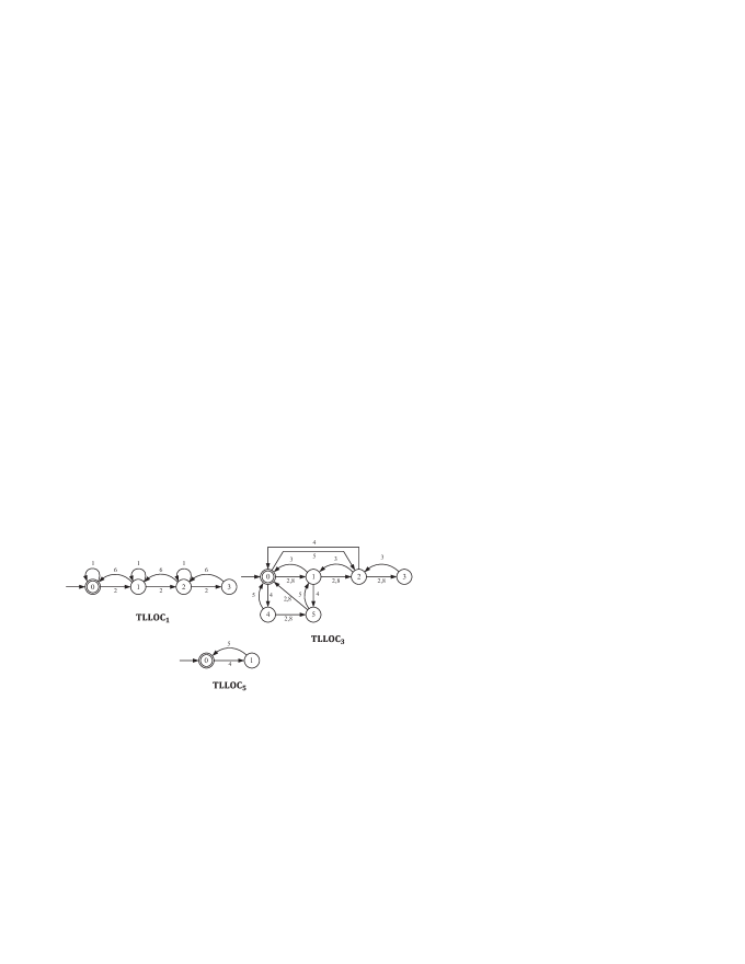
Figure 5: Transfer Line: local controllers with full observation

${\bf TLLOC}_{1}$ for agent $\bf M1$ ensures that no more than three workpieces can be processed in the material-feedback loop. This is realized by counting the occurrences of event 2 (input a workpiece into the loop) and event 6 (output a workpiece from the loop).

${\bf TLLOC}_{3}$ for agent $\bf M2$ guarantees no overflow or underflow of the two buffers. This is realized by counting events 2, 8 (input a workpiece into Buffer1), 3 (output a workpiece from Buffer1), 4 (input a workpiece into Buffer2), and 5 (output a workpiece from Buffer2).

${\bf TLLOC}_{5}$ for agent $\bf TU$ guarantees no overflow or underflow of Buffer2. This is realized by counting event 4 (input a workpiece into Buffer2) and event 5 (output a workpiece from Buffer2).

Now consider partial observation. We consider two cases: first with $\Sigma_{uo}=\{3,6\}$, controlled behavior similar to the full-observation case is achieved but with more complex transition structures; second, with $\Sigma_{uo}=\{1,3,5\}$ (i.e. all controllable events are unobservable), the resulting controlled behavior is more restrictive.

Case (i) $\Sigma_{uo}=\{3,6\}$.We first compute as in (7) the controllable and observable controlled behavior ${\bf SUP1}$ which has 39 states. Then we apply the localization algorithm to obtain the partial-observation local controllers. The results are displayed in Fig. 6. It is verified that the collective controlled behavior of these controllers is equivalent to $\bf SUP1$.

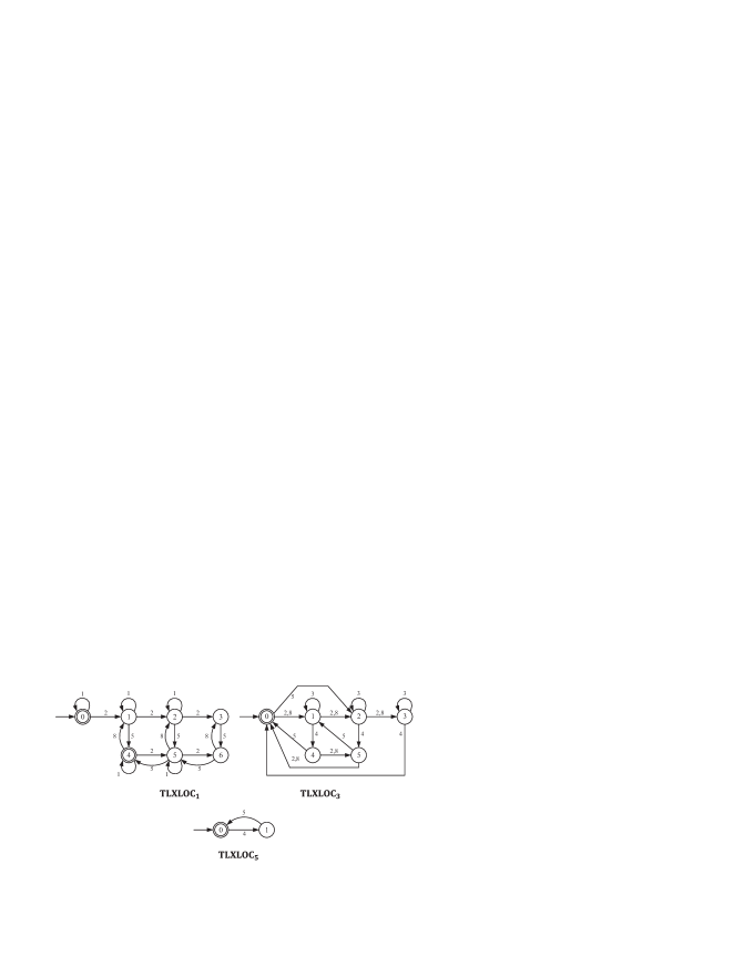
Figure 6: Transfer Line: local controllers under partial observation $P$ ($\Sigma_{uo}=\{3,6\}$)

The control logic of ${\bf TLXLOC}_{1}$ for agent $\bf M1$ is again to ensure that no more than three workpieces can be processed in the loop. But since event 6 is unobservable, the events 5 and 8 instead must be counted so as to infer the occurrences of 6: if 5 followed by 8 is observed, then 6 did not occur, but if 5 is observed and 8 is not observed, 6 may have occurred. As can be seen in Fig. 6, event 6 being unobservable increased the structural complexity of the local controller (as compared to its counterpart in Fig. 5).

The control logic of ${\bf TLXLOC}_{3}$ for agent $\bf M2$ is again to prevent overflow and underflow of the two buffers. But since event 3 is unobservable, instead the occurrences of event 4 must be observed to infer the decrease of content in Buffer1, and at the same time the increase of content in Buffer2. Also note that since the unobservable controllable event 3 is enabled at states 0, 1, 2, 3, we have selfloops of event 3 at those states. The state size of ${\bf TLXLOC}_{3}$ is the same as its counterpart in Fig. 5.

${\bf TLXLOC}_{5}$ for agent $\bf TU$ is identical to the one in the full-observation case.

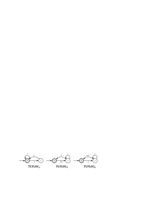
Figure 7: Transfer Line: local controllers under partial observation $P$ ($\Sigma_{uo}=\{1,3,5\}$)

Case (ii) $\Sigma_{uo}=\{1,3,5\}$.We first compute as in (7) the controllable and observable controlled behavior ${\bf SUP2}$ which has only 6 states. Then we apply the localization algorithm to obtain the partial-observation local controllers, as displayed in Fig. 7.

Since all the controllable events are unobservable, the controlled behavior in this case is restrictive: ${\bf TLYLOC}_{1}$ for agent $\bf M1$ allows at most one workpiece to be processed in the loop, and ${\bf TLYLOC}_{2}$ for agent $\bf M2$ allows at most one workpiece to be put in Buffer1 even though Buffer1 has three slots. Also note that in ${\bf TLYLOC}_{5}$ for agent $\bf TU$, since event 5 is unobservable, events 6 and 8 instead must be observed to infer the occurrence of 5: if either 6 or 8 occurs, event 5 must have previously occurred. In spite of the restrictive controlled behavior, these local controllers collectively achieve equivalent controlled performance to the 6-state $\bf SUP2$.

Finally, we allocate each local controller to the agent owning the corresponding controllable event, and according to the transition diagrams of the local controllers, we obtain two communication diagrams one for each case, as displayed in Fig. 8. A local controller either directly observes an event generated by the agent owning it, as denoted by the solid lines in Fig. 8, or imports an event by communication from other local controllers, as denoted by the dashed lines. Although the communication structures are the same in the two diagrams, owing to different observable event sets $\Sigma_{o}$ the observed/communicated events are different.

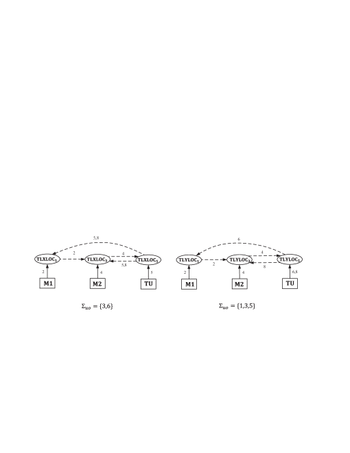
Figure 8: Transfer Line: communication diagrams of local controllers. The solid lines denote that the corresponding events are directly observed by the local controllers; the dashed lines denote that the corresponding events need to be communicated to the local controllers.

V Partial-Observation Localization for Large-Scale Systems

So far we have developed partial-observation supervisor localization assuming that the monolithic supervisor is feasibly computable. This assumption may no longer hold, however, when the system is large-scale and the problem of state explosion arises. In the literature, there have been several architectural approaches proposed to deal with the computational issue based on model abstraction [17, 10, 18, 19].

Just as in [1], for large-scale system, we propose to combine localization with an efficient heterarchical supervisory synthesis approach [10] in an alternative top-down manner: first synthesize a heterarchical array of partial-observation decentralized supervisors and coordinators that collectively achieves globally feasible and nonblocking controlled behavior; then apply the developed localization algorithm to decompose each supervisor/coordinator into local controllers for the relevant agents.

The procedure of this heterarchical supervisor localization under partial observation is outlined as follows:

Step 1) Partial-observation decentralized supervisor synthesis: For each imposed control specification, collect the relevant component agents (e.g. by event-coupling) and compute as in (12) a partial-observation decentralized supervisor.

Step 2) Subsystem decomposition and coordination: After Step 1, we view the system as comprised of a set of modules, each consisting of a decentralized supervisor with its associated component agents. We decompose the system into smaller-scale subsystems, through grouping the modules based on their interconnection dependencies (e.g. event-coupling or control-flow net [10]).

Having obtained a set of subsystems, we verify the nonblocking property for each of them. If a subsystem happens to be blocking, we design a coordinator that removes blocking strings [10, Theorem 4]. The design of the coordinator must respect partial observation; for this reason, we call the coordinator a partial-observation coordinator.

Step 3) Subsystem model abstraction: After Step 2, the system consists of a set of nonblocking subsystems. Now we need to verify the nonconflicting property among these subsystems. For this we use model abstraction with the natural observer property [10] to obtain an abstracted model of each subsystem.

Step 4) Abstracted subsystem decomposition and coordination: This step is similar to Step 2, but for the abstracted models instead of modules. We group the abstracted models based on their interconnection dependencies, and for each group verify the nonblocking property. If a group turns out to be blocking, we design a partial-observation coordinator that removes blocking strings.

Step 5) Higher-level abstraction: Repeat Steps 3 and 4 until there remains a single group of subsystem abstractions in Step 4. The heterarchical supervisor/coordinator synthesis terminates at Step 5; the result is a heterarchical array of partial-observation decentralized supervisors and coordinators. Similar to [10], one can establish that these supervisors/coordinators together achieve globally feasible and nonblocking controlled behavior.

Step 6) Partial-observation localization: In this last step, we apply the partial-observation localization algorithm to decompose each of the obtained decentralized supervisors and coordinators into local controllers for their corresponding controllable events. By Theorem 1, the resulting local controllers achieve the same controlled behavior as the decentralized supervisors and coordinators did, namely the globally feasible and nonblocking controlled behavior.

We note that the above procedure extends the full-observation one in [1] by computing partial-observation decentralized supervisors and coordinators in Steps 1-5, and finally in Step 6 applying the partial-observation supervisor localization developed in Section III. In the following we apply the heterarchical localization procedure to study the distributed control of AGV serving a manufacturing workcell under partial observation. As displayed in Fig. 9, the plant consists of five independent AGV

$${\bf A1},{\bf A2},{\bf A3},{\bf A4},{\bf A5}$$

and there are nine imposed control specifications

$${\bf Z1},{\bf Z2},{\bf Z3},{\bf Z3},{\bf WS13},{\bf WS14S},{\bf WS2},{\bf WS3},{\bf IPS}$$

which require no collision of AGV in the shared zones and no overflow or underflow of buffers in the workstations. The generator models of the plant components and the specification are displayed in Figs. 10 and 11 respectively; the detailed system description and the interpretation of the events are referred to [9, Section 4.7]. Consider partial observation and let the unobservable event set be $\Sigma_{uo}=\{13,23,31,42,53\}$; thus each AGV has an unobservable event. Our control objective is to design for each AGV a set of local strategies such that the overall system behavior satisfies the imposed specifications and is nonblocking.

Figure 9: AGV system configuration. Rectangular dashed boxes represent shared zones of the AGV’s traveling routes.

Figure 10: AGV: Generators of plant components

Figure 11: AGV: Generators of specifications

Step 1) Partial-observation decentralized supervisor synthesis: For each specification displayed in Fig. 11, we group its event-coupled AGV, as displayed in Fig. 12, and synthesize as in (12) a partial-observation decentralized supervisor. The state sizes of these decentralized supervisors are displayed in Table I, in which the supervisors are named correspondingly to the specifications, e.g. $\bf Z1SUP$ is the decentralized supervisor corresponding to the specification $\bf Z1$.

Figure 12: Event-coupling relations

TABLE I: State sizes of partial-observation decentralized supervisors

Supervisor	State size	Supervisor	State size
$\bf Z1SUP$	13	$\bf Z2SUP$	11
$\bf Z3SUP$	26	$\bf Z4SUP$	9
$\bf WS13SUP$	15	$\bf WS14SUP$	19
$\bf WS2SUP$	15	$\bf WS3SUP$	26
$\bf IPSSUP$	13

Step 2) Subsystem decomposition and coordination: We have nine decentralized supervisors, and thus nine modules (consisting of a decentralized supervisor with associated AGV components). Under full observation, the decentralized supervisors for the four zones ($\bf Z1SUP$, …, $\bf Z4SUP$) are harmless to the overall nonblocking property [10], and thus can be safely removed from the interconnection structure; then the interconnection structure of these modules are simplified by applying control-flow net [10]. Under partial observation, however, the four decentralized supervisors are not harmless to the overall nonblocking property and thus cannot be removed. As displayed in Fig. 13, we decompose the overall system into two subsystems:

$${\bf SUB1}:={\bf WS3SUP}||{\bf WS14SUP}||{\bf Z3SUP}||{\bf Z4SUP}$$

$${\bf SUB2}:={\bf WS2SUP}||{\bf WS13SUP}$$

Between the two subsystems are decentralized supervisors $\bf Z1SUP$, $\bf Z2SUP$, and $\bf IPSSUP$. It is verified that $\bf SUB2$ is nonblocking, but $\bf SUB1$ is blocking. Hence we design a coordinator $\bf CO1$ which makes $\bf SUB1$ nonblocking, by

$$L_{m}({\bf CO1})=\sup\mathcal{CO}(L_{m}({\bf SUB1}))$$

adapted from [10, Theorem 4]. This coordinator $\bf CO1$ has 50 states, and we refer to this nonblocking subsystem $\bf NSUB1$.

Figure 13: Subsystem decomposition

Step 3) Subsystem model abstraction: Now we need to verify the nonconflicting property among the nonblocking subsystems ${\bf NSUB1}$, ${\bf SUB2}$ and the decentralized supervisors ${\bf IPSSUP},{\bf Z1SUP}$ and ${\bf Z2SUP}$. First, we determine their shared event set, denoted by $\Sigma_{sub}$. Subsystems ${\bf NSUB1}$ and ${\bf SUB2}$ share all events in $\bf A5$: 50, 51, 52 and 53. For ${\bf IPSSUP},{\bf Z1SUP}$ and ${\bf Z2SUP}$, we use their reduced generator models ${\bf IPSSIM}$, ${\bf Z1SIM}$ and $\bf Z2SIM$ by supervisor reduction [20], as displayed in Fig. 14. By inspection, ${\bf IPSSUP}$ and ${\bf Z1SIM}$ share events 21 and 24 with ${\bf NSUB1}$, and events 11 with ${\bf SUB2}$; ${\bf Z2SUP}$ shares events 24 and 26 with ${\bf NSUB1}$, and events 32, 33 with ${\bf SUB2}$. Thus $\Sigma_{sub}=\{11,12,21,24,26,32,33,50,51,52,53\}$. It is then verified that $P_{sub}:\Sigma^{*}\rightarrow\Sigma_{sub}^{*}$ satisfies the natural observer property [10]. With $P_{sub}$, therefore, we obtain the subsystem model abstractions, denoted by ${\bf QC\_NSUB1}=P_{sub}({\bf NSUB1})$ and ${\bf QC\_SUB2}=P_{sub}({\bf SUB2})$, with state sizes listed in Table II.

TABLE II: State sizes of model abstractions

	$\bf NSUB1$    ${\bf QC\_NSUB1}$	$\bf SUB2$    $\bf QC\_SUB2$
State size	50               19	574           56

Figure 14: Reduced generator models of decentralized supervisors ${\bf Z1SUP}$, ${\bf Z2SUP}$ and ${\bf IPSSUP}$

Step 4) Abstracted subsystem decomposition and coordination: We treat ${\bf QC\_NSUB1}$, ${\bf QC\_SUB2}$, $\bf IPSSIM$, $\bf Z1SIM$ and $\bf Z2SIM$ as a single group, and check the nonblocking property. This group turns out to be blocking, and a coordinator $\bf CO2$ is then designed by

$$L_{m}({\bf CO2})=\sup\mathcal{CO}(L_{m}({\bf QC\_SUB1})||L_{m}({\bf QC\_SUB2})||$$

$$~{}~{}~{}L_{m}({\bf IPSSIM})||L_{m}({\bf Z1SIM})||L_{m}({\bf Z2SIM}))$$

to make the group nonblocking. This coordinator $\bf CO2$ has 160 states.

Step 5) Higher-level abstraction: The modular supervisory control design terminates with the previous Step 4.

We have obtained a hierarchy of nine partial-observation decentralized supervisors and two coordinators. These supervisors and coordinators together achieve globally feasible and nonblocking controlled behavior.

Step 6) Localization: We finally apply the developed supervisor localization procedure to decompose the obtained decentralized supervisors/coordinators into local controllers under partial observation. The generator models of the local controllers are displayed in Fig. 15-19; they are grouped with respect to the individual AGV and their state sizes are listed in Table III. By inspecting the transition structures of the local controllers, only observable events lead to states changes.

TABLE III: State sizes of partial-observation local controllers

	Local controller of	Local controller of	Local controller of	Local controller of	Local controller of
Supervisor/coordinator	$\bf A1(state~{}size)$	$\bf A2(state~{}size)$	$\bf A3(state~{}size)$	$\bf A4(state~{}size)$	$\bf A5(state~{}size)$
$\bf Z1SUP$	$\bf Z1\_11(2)$	$\bf Z1\_21(2)$
$\bf Z2SUP$		$\bf Z2\_21(2)$	$\bf Z2\_33(2)$
$\bf Z3SUP$		$\bf Z3\_21(2)$,$\bf Z3\_23(3)$		$\bf Z3\_41(2)$,$\bf Z3\_43(3)$
$\bf Z4SUP$				$\bf Z4\_41(2)$	$\bf Z4\_51(2)$
$\bf WS13SUP$			$\bf WS13\_31(2)$		$\bf WS13\_51(2)$
$\bf WS14SUP$				$\bf WS14\_43(2)$	$\bf WS14\_51(2)$
$\bf WS2SUP$	$\bf WS2\_13(2)$		$\bf WS2\_33(2)$
$\bf WS3SUP$		$\bf WS3\_21(2)$		$\bf WS3\_41(2)$
$\bf IPSSUP$	$\bf IPS\_11(2)$	$\bf IPS\_21(2)$
$\bf CO1$				$\bf CO1\_41(2)$
$\bf CO2$	$\bf CO2\_11(6)$		$\bf CO2\_33(4)$

Figure 15: Local controllers for $\bf A1$ with controllable events 11 and 13 (the local controllers are named in the format of ‘specification_event’)

Figure 16: Local controllers for $\bf A2$ with controllable events 21 and 23

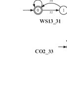
Figure 17: Local controllers for $\bf A3$ with controllable events 31 and 33

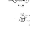
Figure 18: Local controllers for $\bf A4$ with controllable events 41 and 43

Figure 19: Local controllers for $\bf A5$ with controllable events 51 and 53 (event 53 is not disabled and thus there is no corresponding local controller)

Partial observation affects the control logics of the controllers and thus affects the controlled system behavior. For illustration, consider the following case: assuming that event sequence 11.10.13.12.21.18.20.22 has occurred, namely $\bf A1$ has loaded a type 1 part to workstation $\bf WS2$, and $\bf A2$ has moved to input station $\bf IPS2$. Now, $\bf A2$ may load a type 2 part from $\bf IPS2$ (namely, event 23 may occur). Since event 24 ($\bf A2$ exits Zone 1 and re-enter Zone 2) is uncontrollable, to prevent the specification on Zone 2 ($\bf Z2$) not being violated, AGV $\bf A3$ cannot enter Zone 2 if 23 has occurred, i.e. event 33 must be disabled. However, event 33 is eligible to occur if event 23 has occurred. So, under the full observation condition (event 23 is observable) event 33 would occur safely if event 23 has not occurred. However the fact is that event 23 is unobservable; so due to (relative) observability, 33 must also be disabled even if 23 has not occurred, namely the controllers will not know whether or not event 23 has occurred, so it will disabled event 33 in both cases, to prevent the possible illegal behavior. This control strategy coincides with local controller $\bf Z2\_33$: event 33 must be disabled if event 21 has occurred, and will not be re-enabled until event 26 has occurred ($\bf A2$ exits Zone 2 and re-enter Zone 3).

Finally, the heterarchical supervisor localization has effectively generated a set of partial-observation local controllers with small state sizes (between 2 and 6 states). Grouping these local controllers for the relevant AGV, we obtain a distributed control architecture for the system where each AGV is controlled by its own controllers while observing certain observable events of other AGV; according to the transition diagrams of the local controllers, we obtain a communication diagram, as displayed in Fig. 20, which shows the events to be observed (denoted by solid lines) or communicated (denoted by dashed lines) to local controllers.

Figure 20: AGV: communication diagram of local controllers. For $i=1,...,5$, ${\bf LOCi}$ represents the local controllers corresponding to ${\bf Ai}$.

VI Conclusions

We have developed partial-observation supervisor localization to solve the distributed control of multi-agent DES under partial observation. This approach first employs relative observability to compute a partial-observation monolithic supervisor, and then decomposes the supervisor into a set of local controllers whose state changes are caused only by observable events. A Transfer Line example is presented for illustration. When the system is large-scale, we have combined the partial-observation supervisor localization with an efficient heterarchical synthesis procedure. In future research we shall extend the partial-observation localization procedure to study distributed control of timed DES.

References

- [1] K. Cai and W. M. Wonham, “Supervisor localization: a top-down approach to distributed control of discrete-event systems,” IEEE Transactions on Automatic Control, vol. 55, no. 3, pp. 605–618, 2010.
- [2] K. Cai and W. Wonham, “Supervisor localization for large discrete-event systems: case study production cell,” International Journal of Advanced Manufacturing Technology, vol. 50, no. 9-12, pp. 1189–1202, 2010.
- [3] R. Zhang, K. Cai, Y. Gan, Z. Wang, and W. Wonham, “Supervision localization of timed discrete-event systems,” Automatica, vol. 49, no. 9, pp. 2786–2794, 2013.
- [4] K. Cai and W. Wonham, “New results on supervisor localization, with case studies,” Discrete Event Dynamic Systems, vol. 25, no. 1-2, pp. 203–226, 2015.
- [5] K. Cai and W. M. Wonham, Supervisor Localization: A Top-Down Approach to Distributed Control of Discrete-Event Systems. Lecture Notes in Control and Information Sciences, vol. 459, Springer, 2015.
- [6] K. Cai, R. Zhang, and W. Wonham, “Relative observability of discrete-event systems and its supremal sublanguages,” IEEE Transactions on Automatic Control, vol. 60, no. 3, pp. 659–670, 2015.
- [7] F. Lin and W. Wonham, “On observability of discrete-event systems,” Information Sciences, vol. 44, no. 3, pp. 173–198, 1988.
- [8] R. Cieslak, C. Desclaux, A. Fawaz, and P. Varaiya, “Supervisory control of discrete-event processes with partial observations,” IEEE Transactions on Automatic Control, vol. 33, no. 3, pp. 249–260, 1988.
- [9] W. Wonham, Supervisory Control of Discrete-Event Systems. Systems Control Group, ECE Dept, Univ. Toronto, Toronto, ON, Canada, July 2015, available at http://www.control.utoronto.ca/DES.
- [10] L. Feng and W. M. Wonham, “Supervisory control architecture for discrete-event systems,” IEEE Transactions on Automatic Control, vol. 53, no. 6, pp. 1449–1461, 2008.
- [11] S. Takai and T. Ushio, “Effective computation of Lm(G)-closed, controllable, and observable sublanguage arising in supervisory control,” Systems & Control Letters, vol. 49, no. 3, pp. 191–200, 2003.
- [12] X. Yin and S. Lafortune, “Synthesis of maximally permissive supervisors for partially-observed discrete-event systems,” IEEE Transactions on Automatic Control, vol. 61, no. 5, pp. 1239–1254, 2016.
- [13] M. Sampath, S. Lafortune, and D. Teneketzis, “Active diagnosis of discrete-event systems,” IEEE Transactions on Automatic Control, vol. 43, no. 7, pp. 908–929, 1998.
- [14] J. Dubreil, P. Darondeau, and H. Marchand, “Supervisor control for opacity,” IEEE Transactions on Automatic Control, vol. 55, no. 5, pp. 1089–1100, 2010.
- [15] X. Yin and S. Lafortune, “A uniform approach for synthesizing property-enforcing supervisors for partially-observed discrete-event systems,” IEEE Transactions on Automatic Control, 2016, dOI: 10.1109/TAC.2015.2484359.
- [16] C. Cassandras and S. Lafortune, Introduction to Discrete Event Systems, 2nd ed. Springer, 2008.
- [17] R. Hill and D. Tilbury, “Modular supervisory control of discrete-event systems with abstraction and incremental hierarchical construction,” in Proc. 8th International Workshop on Discrete Event Systems, Ann Arbor, MI, July 2006, pp. 399–406.
- [18] K. Schmidt and C. Breindl, “Maximally permissive hierarchical control of decentralized discrete event systems,” IEEE Transactions on Automatic Control, vol. 56, no. 4, pp. 723–737, 2011.
- [19] R. Su, J. H. van Schuppen, and J. E. Rooda, “Maximum permissive coordinated distributed supervisory control of nondeterministic discrete-event systems,” Automatica, vol. 48, no. 7, pp. 1237–1247, 2012.
- [20] R. Su and W. Wonham, “Supervisor reduction for discrete-event systems,” Discrete Event Dynamic Systems, vol. 14, no. 1, pp. 31–53, January 2004.