Graph Estimation for Matrix-variate Gaussian Data

Xi Chen   and   Weidong Liu

Department of Information, Operations & Management Sciences, Stern School of Business

New York University

and   Department of Mathematics, Institute of Natural Sciences and MOE-LSC

Shanghai Jiao Tong University

Abstract: Matrix-variate Gaussian graphical models (GGM) have been widely used for modeling matrix-variate data. Since the support of sparse precision matrix represents the conditional independence graph among matrix entries, conducting support recovery yields valuable information. A commonly used approach is the penalized log-likelihood method. However, due to the complicated structure of precision matrices in the form of Kronecker product, the log-likelihood is non-convex, which presents challenges for both computation and theoretical analysis. In this paper, we propose an alternative approach by formulating the support recovery problem into a multiple testing problem. A new test statistic is developed and based on that, we use the popular Benjamini and Hochberg’s procedure to control false discovery rate (FDR) asymptotically. Our method involves only convex optimization, making it computationally attractive. Theoretically, our method allows very weak conditions, i.e., even when the sample size is finite and the dimensions go to infinity, the asymptotic normality of the test statistics and FDR control can still be guaranteed. We further provide the power analysis result. The finite sample performance of the proposed method is illustrated by both simulated and real data analysis.

Key words and phrases: Correlated samples, false discovery rate, matrix-variate Gaussian graphical models, multiple tests, support recovery

Introduction

In the era of big data, matrix-variate observations are becoming prevalent in a wide range of domains, such as biomedical imaging, genomics, financial markets, spatio-temporal environmental data analysis, and more. A typical example is the gene expression data in genomics, in which each observation contains expression levels of $p$ genes on $q$ microarrays of the same subject (see, e.g., Efron (2009); Yin and Li (2012)). Another example of such data is the multi-channel electroencephalography (EEG) data for brain imaging studies (see, e.g., Bijma et al. (2005)), in which each measurement can be expressed as a matrix with rows corresponding to $p$ different channels and columns to $q$ time points. Leng and Tang (2012) provided more interesting examples of matrix-variate data such as the volatility of equality option. Due to the prevalence of matrix-variate observations (especially high-dimensional observations), it is important for us to understand the structural information encoded in these observations.

To study matrix-variate data where each observation $\mathbf{X}$ is a $p\times q$ matrix, it is commonly assumed that $\mathbf{X}$ follows a matrix-variate Gaussian distribution, e.g., Efron (2009); Allen and Tibshirani (2010); Leng and Tang (2012); Yin and Li (2012); Zhou (2014). The matrix-variate Gaussian distribution is a generalization of the familiar multivariate normal distribution for vector-variate data. In particular, let $\text{vec}(\mathbf{X})\in\mathbb{R}^{pq\times 1}$ be the vectorization of matrix $\mathbf{X}$ obtained by stacking the columns of $\mathbf{X}$ on top of each other. We say that $\mathbf{X}$ follows a matrix-variate Gaussian distribution $\mathbf{X}\sim N(\boldsymbol{\mu},\boldsymbol{\Sigma}\otimes\boldsymbol{\Psi})$ with mean matrix $\boldsymbol{\mu}\in\mathbb{R}^{p\times q}$, row covariance matrix $\boldsymbol{\Sigma}\in\mathbb{R}^{p\times p}$ and column covariance matrix $\boldsymbol{\Psi}\in\mathbb{R}^{q\times q}$ if and only if $\mathrm{vec}(\mathbf{X}^{\prime})\sim N(\mathrm{vec}(\boldsymbol{\mu}^{\prime}),\boldsymbol{\Sigma}\otimes\boldsymbol{\Psi})$, where $\mathbf{X}^{\prime}$ denotes the transpose of $\mathbf{X}$ and $\otimes$ is the Kronecker product.

The readers might refer to Dawid (1981) and Gupta and Nagar (1999) for more properties of matrix-variate Gaussian distribution. Similar to the vector-variate Gaussian graphical models (GGMs) in which the conditional independence graph is encoded in the support of the precision matrix, one can analogously define matrix-variate Gaussian graphical models (MGGM) (a.k.a. Gaussian bigraphical models). Let us denote conditional independence graph by the undirected graph $G=(V,E)$, where $V=\{V_{ij}\}_{1\leq i\leq p,1\leq j\leq q}$ contains $p\times q$ nodes and each node corresponds to an entry in the random matrix $\mathbf{X}$. We can regard the edge set $E$ as a $pq\times pq$ matrix where there is no edge between $X_{ij}$ and $X_{kl}$ if and only if $X_{ij}$ and $X_{kl}$ are conditionally independent given the rest of the entries. The goal of the graph estimation is to estimate the edge set $E$, which unveils important structural information on the conditional independence relationship.

The estimation of the conditional independence graph is equivalent to the estimation of the support of the precision matrix. In particular, let $\boldsymbol{\Omega}=\boldsymbol{\Sigma}^{-1}=(\omega_{ik})_{p\times p}$, $\boldsymbol{\Gamma}=\boldsymbol{\Psi}^{-1}=(\gamma_{jl})_{q\times q}$. The precision matrix of the MGGM is a $pq\times pq$ matrix $\boldsymbol{\Omega}\otimes\boldsymbol{\Gamma}=(\boldsymbol{\Sigma}\otimes\boldsymbol{\Psi})^{-1}$, where $(\boldsymbol{\Omega}\otimes\boldsymbol{\Gamma})_{q(i-1)+j,\;q(k-1)+l}=\omega_{ik}\cdot\gamma_{jl}$. The conditional independence among entries of $\mathbf{X}$ can be presented by the support of $\boldsymbol{\Omega}\otimes\boldsymbol{\Gamma}$ (denoted by $\text{supp}(\boldsymbol{\Omega}\otimes\boldsymbol{\Gamma})$), which is equivalent to $\text{supp}(\boldsymbol{\Omega})\otimes\text{supp}(\boldsymbol{\Gamma})$. To see this, we recall the well-known fact that $X_{ij}$ and $X_{kl}$ are conditionally independent given the rest of the entries, if and only if $\varrho_{ij,kl}=0$, where $\varrho_{ij,kl}$ is the partial correlation between $X_{ij}$ and $X_{kl}$:

$$\varrho_{ij,kl}=-\frac{\omega_{ik}}{\sqrt{\omega_{ii}\omega_{kk}}}\cdot\frac{\gamma_{jl}}{\sqrt{\omega_{jj}\omega_{ll}}}.$$ (1.1)

In other words, $X_{ij}$ and $X_{kl}$ are conditionally independent if and only if there is at least one zero in $\omega_{ik}$ or $\gamma_{jl}$. Therefore, to estimate the conditional independence graph, one only needs to estimate $\text{supp}(\boldsymbol{\Omega})$ and $\text{supp}(\boldsymbol{\Gamma})$. Their Kronecker product $\text{supp}(\boldsymbol{\Omega})\otimes\text{supp}(\boldsymbol{\Gamma})$ gives the edge set $E$. It is worthwhile to note that for a given matrix-variate Gaussian distribution, multiplying a constant to $\boldsymbol{\Omega}$ and dividing $\boldsymbol{\Gamma}$ by the same constant will lead to the same distribution. The existing literature usually assumes that $\omega_{11}=1$ to make the model identifiable (see, e.g., Leng and Tang (2012)). However, if we are interested in support recovery rather than values of $\omega_{ik}$ or $\gamma_{jl}$, then there is no identifiability issue.

Due to the complicated structure in the precision matrices of MGGMs, research on matrix-variate GGMs (MGGMs) is scarce compared to the large body of literature on vector-variate GGMs. The vector-variate GGM with random vector observations can be viewed as a special case of MGGM with $p=1$ or $q=1$ and readers may refer to, e.g., Meinshausen and Bühlmann (2006); Yuan and Lin (2007); Rothman et al. (2008); d’Aspremont et al. (2008); Friedman et al. (2008); Yuan (2010); Ravikumar et al. (2011); Cai et al. (2011); Liu et al. (2012); Xue and Zou (2012); Liu (2013); Zhu et al. (2014); Fan and Lv (2016); Ren et al. (2016) for the recent development in vector-variate GGMs. Among these works, our work is closely related to Liu (2013), which conducts graph estimation via false discovery rate (FDR) control for vector-variate GGMs. However, due to the complicated structure of MGGMs, the proposed test statistics are fundamentally different from the ones in Liu (2013) and the theoretical analysis is much more challenging. The details on the comparisons to Liu (2013) are deferred to Section 6.

For estimating sparse precision matrices of matrix-variate Gaussian data, one popular approach is based on the penalized likelihood method. However, since the precision matrices are in the form of a Kronecker product, the negative log-likelihood function is no longer convex, which makes both computation and theoretical analysis significantly more challenging than in the case of classical vector-variate GGMs. A few recent works (Allen and Tibshirani, 2010; Leng and Tang, 2012; Yin and Li, 2012; Kalaitzis et al., 2013; Tsiligkaridis et al., 2013; Ying and Liu, 2013; Huang and Chen, 2015) have focused on developing various penalized likelihood approaches for estimating MGGMs or extensions of MGGMs (e.g., multiple MGGMs in Huang and Chen (2015) and semiparametric extension in Ying and Liu (2013)). In particular, Leng and Tang (2012) provided pioneering theoretical guarantees on the estimated precision matrices, e.g., rate of convergence under the Frobenius norm and sparsistency. One limitation is that the theoretical results are stated in terms that there exists a local minimizer that enjoys good properties. In practice, it might be difficult to determine whether the obtained local minimizer from an optimization solver is a desired local minimizer. In addition, most convergence results require certain conditions on the sample size $n$ and dimensionality $p$ and $q$, e.g., $p$ and $q$ cannot differ too much from each other and $n$ should go to infinity at a certain rate. On the other hand, we will show later that $n\rightarrow\infty$ is not necessary for the control of false discovery rate (FDR) in support recovery for MGGMs. Zhou (2014) developed new penalized methods for estimating $\boldsymbol{\Sigma}\otimes\boldsymbol{\Psi}$ and $\boldsymbol{\Omega}\otimes\boldsymbol{\Gamma}$ and established the convergence rate under both the spectral norm and the Frobenius norm. However, the main focus of Zhou (2014) is not the support recovery of $\boldsymbol{\Omega}\otimes\boldsymbol{\Gamma}$, and our goal of accurate FDR control cannot be achieved by the method in Zhou (2014) nor other penalized optimization approaches.

The main goal of this work is to infer the support of the precision matrix for an MGGM in the high-dimensional setting, which fully characterizes the conditional independence relationship. Our method differs from the common approaches that turn the problem into a joint optimization over $\boldsymbol{\Omega}$ and $\boldsymbol{\Gamma}$ as penalized likelihood methods. Instead, we utilize the large-scale testing framework and formulate the problem into multiple testing problems for $\boldsymbol{\Omega}$ and $\boldsymbol{\Gamma}$:

$$H^{\boldsymbol{\Omega}}_{0ij}:\omega_{ij}=0\quad\text{vs}\quad H^{\boldsymbol{\Omega}}_{0ij}:\omega_{ij}\neq 0,\quad 1\leq i<j\leq p$$ (1.2)

and

$$H^{\boldsymbol{\Gamma}}_{0ij}:\gamma_{ij}=0\quad\text{vs}\quad H^{\boldsymbol{\Gamma}}_{0ij}:\gamma_{ij}\neq 0,\quad 1\leq i<j\leq q.$$ (1.3)

By conducting the multiple testing for (1.2) and (1.3), we obtain the estimates for the support of $\boldsymbol{\Omega}$ and $\boldsymbol{\Gamma}$, denoted by $\widehat{\mathrm{supp}(\boldsymbol{\Omega})}$ and $\widehat{\mathrm{supp}(\boldsymbol{\Gamma})}$, respectively. Then, the support of $\boldsymbol{\Omega}\otimes\boldsymbol{\Gamma}$ can be naturally estimated by $\widehat{\mathrm{supp}(\boldsymbol{\Omega})}\otimes\widehat{\mathrm{supp}(\boldsymbol{\Gamma})}$. Instead of aiming for perfect support recovery, which will require strong conditions, our goal is to asymptotically control the false discovery rate (FDR). The FDR, originally introduced for multiple testing (Benjamini and Hochberg, 1995), has been considered one of the most important criterion for evaluating the quality of estimated networks (e.g., in the application of genetic data analysis (Schafer and Strimmer, 2005; Ma et al., 2007)). Please refer to (4.25) and (4.28) in Section 4.2 for the definition of FDR in our graph estimation problems.

Although conducting variable selection via multiple testing is not a new idea, how to implement such a high-level idea for MGGMs with a complicated covariance structure requires several innovations in the methodology development. In particular, to conduct the multiple testing in (1.2) and (1.3), it is critical to construct a test statistic with the explicit asymptotic null distribution for each edge. To this end, we propose a new approach that fully utilizes the correlation structures among rows and columns of $\mathbf{X}$. In particular, suppose that there are $n$ i.i.d. $p\times q$ matrix-variate samples $\mathbf{X}^{(1)},\ldots,\mathbf{X}^{(n)}$. To conduct the testing in (1.3) and estimate the support of $q\times q$ matrix $\boldsymbol{\Gamma}$, we treat each row of $\mathbf{X}^{(k)}$ as a $q$-dimensional sample. In such a way, we construct $n\cdot p$ correlated vector-variate samples for the testing problem in (1.3), where the correlation among these “row samples” is characterized by the covariance matrix $\boldsymbol{\Sigma}$. One important advantage of this approach is that it only requires number of row samples $np\rightarrow\infty$ to control FDR asymptotically and thus allows the finite sample size $n$ even when $p$ and $q$ go to infinity. On the other hand, the correlation structure among row samples also presents a significant challenge to the development of the FDR control approach, and most existing inference techniques for vector-variate GGMs heavily rely on the independence assumption (see, e.g., Liu (2013); van de Geer et al. (2014); Ren et al. (2015)). To address this challenge, we summarize the effect of correlation among “row samples” into a simple quantity depending on $\boldsymbol{\Sigma}$, and based on that, introduce a variance correction technique into the construction of the test statistics (see Section 3.1). It is noteworthy that the testing of the $\text{supp}(\boldsymbol{\Omega})$ in (1.2) can be performed in a completely symmetric way with $nq$ correlated “column samples” from the data.

More specifically, the high-level description of the proposed large-scale testing approach is as follows. Given the “row samples” from the data, the first step is to construct an asymptotically normal test statistic for each $H_{0ij}^{\boldsymbol{\Gamma}}$ in (1.3). We utilize a fundamental result from multivariate analysis which relates the partial correlation coefficient to the correlation coefficient of residuals from linear regression. To compute the sample version of the correlation coefficient of the residuals, we first construct an initial estimator for the regression coefficients. With the initial estimator in place, we can directly show that the sample correlation coefficient of the residuals is asymptotically normal under the null. We further apply the aforementioned variance correction technique and obtain the final test statistic for each $H_{0ij}^{\boldsymbol{\Gamma}}$. Combining the developed test statistics with the Benjamini and Hochberg approach (Benjamini and Hochberg, 1995), we show that the resulting procedure asymptotically controls the FDR for both $\widehat{\mathrm{{\mathrm{supp}}}(\boldsymbol{\Gamma})}$ and $\widehat{\mathrm{{\mathrm{supp}}}(\boldsymbol{\Omega})}$ (and thus $\widehat{\mathrm{{\mathrm{supp}}}(\boldsymbol{\Gamma})}\otimes\widehat{\mathrm{{\mathrm{supp}}}(\boldsymbol{\Omega})}$) under some sparsity conditions of $\boldsymbol{\Gamma}$ and $\boldsymbol{\Omega}$.

The proposed method described above is the first to investigate FDR control in MGGMs. This work greatly generalizes the method on FDR control for i.i.d. vector-variate GGMs in Liu (2013) and improves over optimization-based approaches. The main contribution and difference between our results and the existing ones for vector-variate GGMs (e.g., Liu (2013)) are summarized as follows,

1. We propose a novel test statistic in Section 3.1. By introducing a new construction of the initial regression coefficients (i.e., setting a particular element in each initial Lasso estimator to zero), our testing approach no longer requires a complicated bias-correlation step as in Eq. (6) in Liu (2013). Furthermore, the limiting null distribution of the sample covariance coefficient between residuals (see $\widehat{r}_{ij}$ in (3.10)) can be easily obtained. In fact, this idea can be used to provide simpler testing procedure for ordinary vector-variate high-dimensional graphical models.

2. Instead of relying on the i.i.d. assumption in GGM literature, we propose to extract $np$ correlated vector-variate “rows samples” (as well $nq$ correlated “column samples”) from matrix-variate observations. By utilizing correlation structure among rows and columns, our approach allows for finite sample size, which is a very attractive property from both theoretical and practical perspectives. More specifically, even in the case that $n$ is a constant and $p\rightarrow\infty$ and $q\rightarrow\infty$, our method still guarantees the asymptotic normality of the test statistics and FDR control. This is fundamentally different from the case of vector-variate GGMs, which always requires $n\rightarrow\infty$ for the support recovery. Therefore, this work greatly generalizes Liu (2013), which only deals with i.i.d. vector-variate Gaussian samples, to correlated data.

   In this paper, we developed new techniques and theoretical analysis to address the challenges arising from correlated samples. For example, the proposed variance correlation technique can be used as a general technique for high-dimensional inference with correlated samples. Moreover, the initial estimator is now based on the Lasso with correlated samples. To this end, we establish the consistency result for the Lasso with correlated samples, which itself is of independent interest for high-dimensional linear regression.

3. Theoretically, by utilizing the Kronecker product structure of the covariance matrix of X, the proposed method allows the partial correlation between $X_{ij}$ and $X_{kl}$ (i.e., $\varrho_{ij,kl}$ in (1.1)) to be of the order of $\frac{1}{n-1}\sqrt{\frac{\log p\log q}{pq}}$ so that the corresponding edge can be detected (please see the power analysis in Section 4.3 and Theorem 4 for details.) This is essentially different from any vector-variate GGM estimator (e.g., the one from Liu (2013)) that requires the partial correlation to be at least $C\frac{1}{\sqrt{n}}$.

Moreover, in terms of support recovery and computation cost, the proposed method has several advantages as compared to popular penalized likelihood approaches:

1. As we mentioned before, the FDR is a basic performance measure of support recovery of MGGMs. The proposed method provides an accurate control of FDR (see Theorem 3); however, the existing optimization-based approaches remain unclear about how to choose the tuning parameter to control a desired FDR while keeping nontrivial statistical power. In fact, existing support recovery results only guarantee that the estimated positions of zeros are supersets of the positions of true zeros in $\boldsymbol{\Omega}$ and $\boldsymbol{\Gamma}$ with probability tending to one when $n,p,q$ all go to infinity at certain rates. (see, e.g., Leng and Tang (2012); Yin and Li (2012)).

2. In terms of computation, as compared to existing penalized likelihood methods whose objective functions are non-convex, our approach is completely based on convex optimization and thus computationally more attractive. In particular, the main computational cost of our approach is the construction of initial estimates for $p+q$ regression coefficient vectors, which will directly lead to our test statistics. The corresponding computational problems are completely independent allowing an efficient parallel implementation.

3. Theoretically, our approach allows a wider range of $p$ and $q$. In particular, our result on FDR control holds for $(p,q)$ such that $q^{r_{2}}\leq p\leq q^{r_{1}}$ for some $0<r_{2}\leq r_{1}$, while in comparison, Leng and Tang (2012) require that $p\log(p)=o(nq)$ and $q\log(q)=o(np)$. As one can see, if $n$ is a constant or $n\rightarrow\infty$ but $n=o(\min(\log p,\log q))$, such a condition will not hold.

Notations and Organization of the paper

We introduce some necessary notations. Let $\mathbf{X}^{(k)}=(X^{(k)}_{ij})_{p\times q}$ for $k=1,\ldots,n\;$ be the $n$ i.i.d. matrix-variate observations from $N_{p,q}(\boldsymbol{\mu},\boldsymbol{\Sigma}\otimes\boldsymbol{\Psi})$ and let $\bar{\mathbf{X}}=\frac{1}{n}\sum_{k=1}^{n}\mathbf{X}^{(k)}$. Put $\boldsymbol{\Sigma}=(\sigma_{ij})$ and $\boldsymbol{\Psi}=(\psi_{ij})$. For any vector $\mathbf{x}=(x_{1},\ldots,x_{p})^{{}^{\prime}}$, let $\mathbf{x}_{-i}$ denote $p-1$ dimensional vector by removing $x_{i}$ from $\mathbf{x}$. Let $\langle\mathbf{x},\mathbf{y}\rangle$ be the inner product of two vectors $\mathbf{x}$ and $\mathbf{y}$. For any $p\times q$ matrix $\mathbf{A}$, let $\mathbf{A}_{i,\cdot}$ denote the $i$-th row of $\mathbf{A}$ (or $\mathbf{A}_{i}$ when it is clear from the context) and $\mathbf{A}_{\cdot,j}$ denote the $j$-th column of $\mathbf{A}$ (or $\mathbf{A}_{j}$ when it is clear from the context). Further, let $\mathbf{A}_{i,-j}$ denote the $i$-th row of $\mathbf{A}$ with its $j$-th entry being removed and $\mathbf{A}_{-i,j}$ denotes the $j$-th column of $\mathbf{A}$ with its $i$-th entry being removed. $\mathbf{A}_{-i,-j}$ denote a $(p-1)\times(q-1)$ matrix by removing the $i$-th row and $j$-th column of $\mathbf{A}$. Define $[n]=\{1,\ldots,n\}$, $[p]=\{1,\ldots,p\}$ and $[q]=\{1,\ldots,q\}$. For a $p$-dimensional vector $\mathbf{x}$, let $|\mathbf{x}|_{0}=\sum_{j=1}^{p}I(x_{j}\neq 0)$, $|\mathbf{x}|_{1}=\sum_{j=1}^{p}|x_{j}|$ and $|\mathbf{x}|_{2}=\sqrt{\sum_{j=1}^{p}x_{j}^{2}}$ be the $\ell_{0}$, $\ell_{1}$ and Euclidean norm of $\mathbf{x}$, respectively. For a matrix $\mathbf{A}=(a_{ij})\in\mathbb{R}^{p\times q}$, let $\|\mathbf{A}\|_{\text{F}}=\sqrt{\sum_{i\in[p],j\in[q]}a_{ij}^{2}}$ be the Frobenius norm of $\mathbf{A}$, $|\mathbf{A}|_{\infty}=\max_{i\in[p],j\in[q]}|a_{ij}|$ be the element-wise $\ell_{\infty}$-norm of $\mathbf{A}$ and $\|\mathbf{A}\|_{2}=\sup_{|\mathbf{x}|_{2}\leq 1}|\mathbf{A}\mathbf{x}|_{2}$ be the spectral norm of $\mathbf{A}$. For a square matrix $\mathbf{A}$, let $\text{tr}(\mathbf{A})$ denote the trace of $\mathbf{A}$. For a given set $\mathcal{H}$, let $Card(\mathcal{H})$ be the cardinality of $\mathcal{H}$. Throughout the paper, we use $\mathbf{I}_{p}$ to denote the $p\times p$ identity matrix, and use $C$, $c$, etc. to denote generic constants whose values might change from place to place.

The rest of the paper is organized as follows. In Section 3, we introduce our test statistics and then describe the FDR control procedure for MGGM estimation. Theoretical results on asymptotic normality of our test statistic and FDR control are given in Section 4. Simulations and real data analysis are given in Section 5. In Section 6, we provide further discussions on the proposed method and also point out some interesting future work. All of the technical proofs and some additional experimental results are relegated to the supplementary material.

Methodology

Recall the definition of false discover proportion (FDP) as the proportion of false discoveries among total rejections. Note that, if $\widehat{\text{supp}(\boldsymbol{\Omega})}$ and $\widehat{\text{supp}(\boldsymbol{\Gamma})}$ are the estimators of supp$(\boldsymbol{\Omega})$ and supp$(\boldsymbol{\Gamma})$, respectively, under the control of FDP at level $\alpha\in[0,1]$, it is clear that the FDP of $\widehat{\text{supp}(\boldsymbol{\Omega})}\otimes\widehat{\text{supp}(\boldsymbol{\Gamma})}$ as an estimator of supp($\boldsymbol{\Omega}\otimes\boldsymbol{\Gamma}$) will be controlled at some level $\alpha{{}^{\prime}}$. Here, the level $\alpha^{\prime}$ (explicitly given later in (4.32)) is a monotonically increasing function in $\alpha$. Therefore, we reduce our task to design an estimator of supp$(\boldsymbol{\Gamma})$ under the FDP level $\alpha$ and the estimator of supp$(\boldsymbol{\Omega})$ can be constructed in a completely symmetric way. We propose to estimate supp$(\boldsymbol{\Gamma})$ by implementing the following large-scale multiple tests:

$$H_{0ij}:\gamma_{ij}=0\quad\mbox{vs.}\quad H_{1ij}:\gamma_{ij}\neq 0,\quad 1\leq i<j\leq q.$$ (3.4)

Construction of test statistics

In this section, we propose our test statistic for each $H_{0ij}$ in (3.4) constructed from $n$ i.i.d. $p\times q$ matrix-variate samples $\mathbf{X}^{(1)},\ldots,\mathbf{X}^{(n)}$ with the population distribution $\mathbf{X}\sim N(\boldsymbol{\mu},\boldsymbol{\Sigma}\otimes\boldsymbol{\Psi})$. Let us denote the partial correlation matrix associated with $\boldsymbol{\Gamma}$ by $\boldsymbol{\rho}^{\boldsymbol{\Gamma}}=\left(\rho^{\boldsymbol{\Gamma}}_{ij\cdot}\right)_{q\times q}$, where each $\rho^{\boldsymbol{\Gamma}}_{ij\cdot}=-\frac{\gamma_{ij}}{\sqrt{\gamma_{ii}\gamma_{jj}}}$ is the partial correlation coefficient between $X_{li}$ and $X_{lj}$ for any $1\leq l\leq p$. The following well-known result relates the partial correlation coefficient $\rho^{\boldsymbol{\Gamma}}_{ij\cdot}$ to regression problems. In particular, for $1\leq i<j\leq q$ and any $1\leq l\leq p$, let us define the population regression coefficients:

$$(\alpha_{i},\boldsymbol{\beta}_{i}) =\mathop{\rm arg\min}_{a\in\mathbb{R},\mathbf{b}\in\mathbb{R}^{q-1}}\mathbb{E}(X_{li}-a-\mathbf{X}_{l,-i}\mathbf{b})^{2}\;,(\alpha_{j},\boldsymbol{\beta}_{j}) =\mathop{\rm arg\min}_{a\in\mathbb{R},\mathbf{b}\in\mathbb{R}^{q-1},}\mathbb{E}(X_{lj}-a-\mathbf{X}_{l,-j}\mathbf{b})^{2}.$$ (3.5)

The standard linear regression result shows that

$$\boldsymbol{\beta}_{i}=-\gamma^{-1}_{ii}\boldsymbol{\Gamma}_{-i,i}\;;\qquad\boldsymbol{\beta}_{j}=-\gamma^{-1}_{jj}\boldsymbol{\Gamma}_{-j,j}.$$ (3.6)

For such defined $\boldsymbol{\beta}_{i}$ and $\boldsymbol{\beta}_{j}$, the corresponding residuals $\epsilon_{li}$ and $\epsilon_{lj}$ take the following form,

$$\varepsilon_{li}=X_{li}-\alpha_{i}-\mathbf{X}_{l,-i}\boldsymbol{\beta}_{i}\;;\quad\varepsilon_{lj}=X_{lj}-\alpha_{j}-\mathbf{X}_{l,-j}\boldsymbol{\beta}_{j}.$$ (3.7)

It is known that $\mathbb{E}(\varepsilon_{li})=\mathbb{E}(\varepsilon_{lj})=0$. Moreover, the correlation between $\varepsilon_{li}$ and $\varepsilon_{lj}$ is $\text{Corr}(\varepsilon_{li},\varepsilon_{lj})=-\rho^{\boldsymbol{\Gamma}}_{ij\cdot}=\frac{\gamma_{ij}}{\sqrt{\gamma_{ii}\gamma_{jj}}}$. To see this, let $\boldsymbol{\gamma}_{i}$ be the $i$-th column of $\boldsymbol{\Gamma}$ for $1\leq i\leq q$. By (3.6) and (3.7), we can equivalently write $\epsilon_{li}=-\alpha_{i}+\gamma_{ii}^{-1}\mathbf{X}_{l,\cdot}\boldsymbol{\gamma}_{i}$ and $\epsilon_{lj}=-\alpha_{j}+\gamma_{jj}^{-1}\mathbf{X}_{l,\cdot}\boldsymbol{\gamma}_{j}$. Since the covariance of $\mathbf{X}_{l,\cdot}$, $\text{Cov}(\mathbf{X}_{l,\cdot})$, is $\sigma_{ll}\boldsymbol{\Psi}=\sigma_{ll}\boldsymbol{\Gamma}^{-1}$, we have

$$\mathrm{Cov}(\epsilon_{li},\epsilon_{lj})=\gamma_{ii}^{-1}\gamma_{jj}^{-1}\boldsymbol{\gamma}_{i}^{T}\text{Cov}(\mathbf{X}_{l,\cdot})\boldsymbol{\gamma}_{j}=\sigma_{ll}\gamma_{ii}^{-1}\gamma_{jj}^{-1}\left(\boldsymbol{\gamma}_{i}^{T}\boldsymbol{\Gamma}^{-1}\right)\boldsymbol{\gamma}_{j}=\sigma_{ll}\gamma_{ii}^{-1}\gamma_{jj}^{-1}\gamma_{ij},$$ (3.8)

where the last equality is because $\boldsymbol{\gamma}_{i}^{T}\boldsymbol{\Gamma}^{-1}=\mathbf{e}_{i}^{T}$ and $\mathbf{e}_{i}$ denotes the $i$-th canonical vector. Similarly, we obtain that $\mathrm{Var}(\epsilon_{li})=\sigma_{ll}\gamma_{ii}^{-1}$ and $\mathrm{Var}(\epsilon_{lj})=\sigma_{ll}\gamma_{jj}^{-1}$, which together with (3.8) imply that $\text{Corr}(\varepsilon_{li},\varepsilon_{lj})=\frac{\gamma_{ij}}{\sqrt{\gamma_{ii}\gamma_{jj}}}$. Therefore, testing whether $\gamma_{ij}=0$ (or $\rho^{\boldsymbol{\Gamma}}_{ij\cdot}=0$) is equivalent to testing whether $\text{Corr}(\varepsilon_{li},\varepsilon_{lj})=0$. We will build our test statistics based on this key equivalence relationship.

To implement the aforementioned idea, one needs to construct an initial estimator for each $\boldsymbol{\beta}_{j}$ so that the distribution of sample correlation coefficient of residuals can be deduced easily. To construct the initial estimator, we first let $\widehat{\boldsymbol{\beta}}_{j}=(\widehat{\beta}_{1,j},\ldots,\widehat{\beta}_{q-1,j})^{{}^{\prime}}$ be any estimator for $\boldsymbol{\beta}_{j}$, which satisfies

$$\max_{1\leq j\leq q}|\widehat{\boldsymbol{\beta}}_{j}-\boldsymbol{\beta}_{j}|_{1}=O_{\mathbb{P}}(a_{n1}),\quad\mbox{and}\quad\max_{1\leq j\leq q}|\widehat{\boldsymbol{\beta}}_{j}-\boldsymbol{\beta}_{j}|_{2}=O_{\mathbb{P}}(a_{n2}),$$ (3.9)

where $a_{n1}\rightarrow 0$ and $a_{n2}\rightarrow 0$ at some rate that will be specified later. The Lasso (Tibshirani, 1996), Dantzig selector (Candès and Tao, 2007), or other sparse regression approaches can be adopted provided that (3.9) is satisfied (see Section 3.2 for details). Under the null $H_{0ij}$: $\gamma_{ij}=0$, according to (3.6), the $i$-th element in $\boldsymbol{\beta}_{j}$, which corresponds to the covariate $X_{li}$ in (3.7), is zero; and the $(j-1)$-th element in $\boldsymbol{\beta}_{i}$ which corresponds to the covariate $X_{lj}$ in (3.7), is also zero. Hence, for each pair $i<j$, we construct the initial estimators $\widehat{\boldsymbol{\beta}}_{j,\backslash i}=(\widehat{\boldsymbol{\beta}}_{1,j},\ldots,\widehat{\boldsymbol{\beta}}_{i-1,j},0,\widehat{\boldsymbol{\beta}}_{i+1,j},\ldots,\widehat{\boldsymbol{\beta}}_{q-1,j})^{{}^{\prime}}$ and $\widehat{\boldsymbol{\beta}}_{i,\backslash j}=(\widehat{\boldsymbol{\beta}}_{1,i},\ldots,\widehat{\boldsymbol{\beta}}_{j-2,i},0,\widehat{\boldsymbol{\beta}}_{j,i},\ldots,\widehat{\boldsymbol{\beta}}_{q-1,i})^{{}^{\prime}}$ for $\boldsymbol{\beta}_{j}$ and $\boldsymbol{\beta}_{i}$, respectively. For notation briefness, we let $\widehat{\boldsymbol{\beta}}_{j,\backslash j}=\widehat{\boldsymbol{\beta}}_{j}$ so that the “sample residual” $\widehat{\varepsilon}^{(k)}_{ljj}$ introduced in the below is also well-defined (see (3.10)).

Given the initial estimators under the null, we construct the “sample residuals” by treating each row $l\in[p]$ of a matrix-variate observation $\mathbf{X}^{(k)}$ for $k\in[n]$ as a “row sample”, i.e., $\mathbf{X}^{(k)}_{l,\cdot}=(X^{(k)}_{l1},\ldots X^{(k)}_{lq})$. The “sample residuals” corresponding to $\epsilon_{li}$ and $\epsilon_{lj}$ in (3.7) are defined as follows:

$$\widehat{\varepsilon}^{(k)}_{lij}=X^{(k)}_{li}-\bar{X}_{li}-(\textbf{X}^{(k)}_{l,-i}-\bar{\textbf{X}}_{l,-i})\widehat{\boldsymbol{\beta}}_{i,\setminus j},\quad\widehat{\varepsilon}^{(k)}_{lji}=X^{(k)}_{lj}-\bar{X}_{lj}-(\textbf{X}^{(k)}_{l,-j}-\bar{\textbf{X}}_{l,-j})\widehat{\boldsymbol{\beta}}_{j,\setminus i},$$ (3.10)

where $\bar{X}_{li}=\frac{1}{n}\sum_{k=1}^{n}X^{(k)}_{li}$ and $\bar{\textbf{X}}_{l,-i}=\frac{1}{n}\sum_{k=1}^{n}\textbf{X}^{(k)}_{l,-i}$. Further let $\widehat{r}_{ij}$ be the sample covariance coefficient between constructed residuals,

$$\widehat{r}_{ij}=\frac{1}{(n-1)p}\sum_{k=1}^{n}\sum_{l=1}^{p}\widehat{\varepsilon}^{(k)}_{lij}\widehat{\varepsilon}^{(k)}_{lji};$$ (3.11)

and $\frac{\widehat{r}_{ij}}{\sqrt{\widehat{r}_{ii}\widehat{r}_{jj}}}$ be the corresponding sample correlation coefficient of residuals.

The proposed construction of the sample correlation of residuals has twofold benefits. First, under the null $H_{0ij}$, incorporating the fact that $\gamma_{ij}=0$ into the regression coefficients enables us to derive the asymptotic null distribution of the sample correlation coefficients. In particular, later in Proposition 1, we show that under the null,

$$\sqrt{\frac{(n-1)p}{A_{p}}}\frac{\widehat{r}_{ij}}{\sqrt{\widehat{r}_{ii}\widehat{r}_{jj}}}\Rightarrow N(0,1),$$ (3.12)

where

$$A_{p}=\frac{p\|\boldsymbol{\Sigma}\|^{2}_{\text{F}}}{(\text{tr}(\boldsymbol{\Sigma}))^{2}}.$$ (3.13)

Here, $A_{p}$ is the asymptotic variance of $\sqrt{(n-1)p}\frac{\widehat{r}_{ij}}{\sqrt{\widehat{r}_{ii}\widehat{r}_{jj}}}$ under the null. It is noteworthy that the term $A_{p}$ is critical since it plays the role of variance correction when treating rows of matrix-variate data as correlated samples. The second merit of the proposed construction is that, although the sample correlation coefficients are constructed under the null, we can show that $\frac{\widehat{r}_{ij}}{\sqrt{\widehat{r}_{ii}\widehat{r}_{jj}}}$ converges to $(1-\gamma_{ij}\psi_{ij})\rho^{\boldsymbol{\Gamma}}_{ij\cdot}$ in probability as $np\rightarrow\infty$ under both the null and alternative (see Proposition 2). This result indicates that the test statistic based on $\frac{\widehat{r}_{ij}}{\sqrt{\widehat{r}_{ii}\widehat{r}_{jj}}}$ can properly reject the null when the magnitude of partial correlation coefficient $|\rho^{\boldsymbol{\Gamma}}_{ij\cdot}|$ is away from zero. It is worth noting that for many widely studied covariance structures of $\boldsymbol{\Psi}$ and $\boldsymbol{\Gamma}=\boldsymbol{\Psi}^{-1}$, the quantity $\psi_{ij}\gamma_{ij}$ is often non-positive, which makes the signal strength $(1-\gamma_{ij}\psi_{ij})\rho^{\boldsymbol{\Gamma}}_{ij\cdot}$ even larger than the partial correlation coefficient and thus leads to good statistical power. For example, for two variables which are directly positively/negatively correlated, they will often be positively/negatively conditional correlated.

It is worthwhile to note that the variance correction quantity $A_{p}\in\mathbb{R}$ in (3.12) is unknown as it involves $\boldsymbol{\Sigma}$. In the next subsection, we will propose a ratio consistent estimator $\widehat{A}_{p}$ such that $\widehat{A}_{p}/A_{p}\rightarrow 1$ in probability as $nq\rightarrow\infty$. Using the estimator $\widehat{A}_{p}$, we construct the final test statistic for $H_{0ij}$:

$$\widehat{T}_{ij}=\sqrt{\frac{(n-1)p}{\widehat{A}_{p}}}\frac{\widehat{r}_{ij}}{\sqrt{\widehat{r}_{ii}\widehat{r}_{jj}}},$$ (3.14)

which is asymptotically normal given (3.12) and the ratio consistency of $\widehat{A}_{p}$.

Estimator for $A_{p}$

We propose an estimator $\widehat{A}_{p}$ of $A_{p}$ based on a thresholding estimator of $\boldsymbol{\Sigma}$. We first construct an initial estimator of $\boldsymbol{\Sigma}$ based on $nq$ “column samples”, where each column of $\mathbf{X}^{(k)}$ for $k\in[n]$ is treated as a $p$-dimensional sample. In particular, let $\bar{\textbf{X}}=\frac{1}{n}\sum_{k=1}^{n}\textbf{X}^{(k)}$, each centered column sample $\mathbf{Y}_{kj}=\mathbf{X}_{\cdot,j}^{(k)}-\bar{\mathbf{X}}_{\cdot,j}\in\mathbb{R}^{p\times 1}$ for $k\in[n]$ and $j\in[q]$. Moreover, let us define $\widehat{\boldsymbol{\Sigma}}=(\widehat{\sigma}_{ij})_{p\times p}:=\frac{1}{(n-1)q}\sum_{k=1}^{n}\sum_{j=1}^{q}(\mathbf{Y}_{kj})(\mathbf{Y}_{kj})^{\prime}$. In a more succinct notation, let $\textbf{Y}=[\textbf{X}^{(1)}-\bar{\textbf{X}},\ldots,\textbf{X}^{(n)}-\bar{\textbf{X}}]\in\mathbb{R}^{p\times(nq)}$and $\widehat{\boldsymbol{\Sigma}}=\frac{1}{(n-1)q}\textbf{Y}\textbf{Y}^{\prime}$. Then, we threshold the elements of $\widehat{\boldsymbol{\Sigma}}$ as follows:

$$\widehat{\sigma}_{ij,\lambda}=\widehat{\sigma}_{ij}I\left\{|\widehat{\sigma}_{ij}|\geq\lambda\sqrt{\frac{\log\max(p,nq)}{nq}}\right\}\quad\text{for}\;i\neq j;$$ (3.15)

and $\widehat{\sigma}_{ii,\lambda}=\widehat{\sigma}_{ii}$ for $i\in[p]$. Set $\widehat{\boldsymbol{\Sigma}}_{\lambda}=(\widehat{\sigma}_{ij,\lambda})_{p\times p}$ and define the plug-in estimator of $A_{p}$:

$$\widehat{A}_{p}=\frac{p\|\widehat{\boldsymbol{\Sigma}}_{\lambda}\|^{2}_{\text{F}}}{(\text{tr}(\widehat{\boldsymbol{\Sigma}}_{\lambda}))^{2}}.$$ (3.16)

In Proposition 3 in Section 4, we show that $\widehat{A}_{p}/A_{p}\rightarrow 1$ in probability as $nq\rightarrow\infty$ for a properly chosen $\lambda$ (a data-driven approach for the choice of $\lambda$ will be discussed later in Section 3.2). Therefore, by (3.12), we have the desired asymptotic normality of $\widehat{T}_{ij}$ under the null: $\widehat{T}_{ij}\Rightarrow N(0,1)$ as $np\rightarrow\infty$.

We further note that when the columns of X are i.i.d. (i.e., $\boldsymbol{\Psi}=\mathbf{I}_{q})$, consistency under the spectral norm $\|\widehat{\boldsymbol{\Sigma}}_{\lambda}-\boldsymbol{\Sigma}\|_{2}$ has been established if the sparsity condition of $\boldsymbol{\Sigma}$ satisfies the row sparsity level $s_{0}(p)=O(\sqrt{nq/\log p})$ (see, e.g., Bickle and Levina (2008); Cai and Liu (2011) and references therein). We do not need such a strong consistency result of $\widehat{\boldsymbol{\Sigma}}_{\lambda}$ in the spectral norm to establish the consistency of $\widehat{A}_{p}$. In fact, since $A_{p}$ only involves $\|\boldsymbol{\Sigma}\|_{\text{F}}$ rather than $\boldsymbol{\Sigma}$ itself, the sparsity condition on $s_{0}(p)$ is no longer necessary; see Proposition 3 and its proof for more details. It is also noteworthy that some other estimators of $\|\boldsymbol{\Sigma}\|_{\text{F}}$ have been proposed (e.g,. by Chen and Qin (2010)). However, those approaches heavily rely on the i.i.d. assumption on the columns of X, which is not valid in our setting.

Initial estimators of regression coefficients

In the construction of the test statistic $\widehat{T}_{ij}$, we need the estimate $\widehat{\boldsymbol{\beta}}_{j}$ that satisfies the condition in (3.9). Here, we choose to construct $\widehat{\boldsymbol{\beta}}_{j}$ using Lasso for the presentation simplicity, however other approaches such as the Dantzig selector can also be used. In particular, let $\textbf{Z}=\left[(\textbf{X}^{(1)})^{\prime}-\bar{\textbf{X}}^{{}^{\prime}},\ldots,(\textbf{X}^{(n)})^{\prime}-\bar{\textbf{X}}^{{}^{\prime}}\right]\in\mathbb{R}^{q\times(np)}$ be $np$ $q$-dimensional samples extracted from the data, and $\widehat{\boldsymbol{\Psi}}=\frac{1}{(n-1)p}\textbf{Z}\textbf{Z}^{{}^{\prime}}=:(\widehat{\psi}_{ij})_{q\times q}$. For $1\leq j\leq q$, define the scaling/normalizing vector $\mathbf{D}_{j}={\mathrm{diag}}(\widehat{\boldsymbol{\Psi}}_{-j,-j})\in\mathbb{R}^{(q-1)\times(q-1)}$. The coefficients $\boldsymbol{\beta}_{j}$ can be estimated by Lasso as follows:

$$\widehat{\boldsymbol{\beta}}_{j}(\delta)=\mathbf{D}_{j}^{-1/2}\widehat{\boldsymbol{\alpha}}_{j}(\delta),$$ (3.17)

where

$$\widehat{\boldsymbol{\alpha}}_{j}(\delta)=\mathop{\rm arg\min}_{\boldsymbol{\alpha}\in\mathbb{R}^{q-1}}\Big{\{}\frac{1}{2np}\sum_{k=1}^{n}\sum_{l=1}^{p}(X^{(k)}_{lj}-\bar{X}_{lj}-(\textbf{X}^{(k)}_{l,-j}-\bar{\textbf{X}}_{l,-j})\mathbf{D}_{j}^{-1/2}\boldsymbol{\alpha})^{2}+\theta_{nj}(\delta)|\boldsymbol{\alpha}|_{1}\Big{\}}$$ (3.18)

and

$$\theta_{nj}(\delta)=\delta\sqrt{\frac{\widehat{\psi}_{jj}\log\max(q,np)}{np}}.$$ (3.19)

In the Lasso estimate in (3.18), the $np$ covariates-response pairs $\left(\textbf{X}^{(k)}_{l,-j}-\bar{\textbf{X}}_{l,-j}\;,\;X^{(k)}_{lj}-\bar{X}_{lj}\right)$ for $k\in[n]$ and $j\in[p]$ are not i.i.d. and thus the standard consistency result of Lasso cannot be applied here. By exploring the correlation structure among rows of $\mathbf{X}$, we managed to derive the rate of convergence of the Lasso estimator in the $\ell_{1}$ and the $\ell_{2}$ norms. This result (see Proposition 4 and its proof) might be of independent interest for dealing with high-dimensional correlated data. For the choice of tuning parameters, our theoretical results will hold for any large enough constants $\lambda$ in (3.15) for estimating $\widehat{A}_{p}$ (see Proposition 3) and $\delta>0$ in (3.19) for $\widehat{\boldsymbol{\beta}}_{j}(\delta)$ (see Proposition 4). In our experiment, we will adopt a data-driven parameter-tuning strategy from Liu (2013).

FDR control procedure

Given the constructed test statistic $\widehat{T}_{ij}$, we can carry out $(q^{2}-q)/2$ tests in (3.4) simultaneously using the popular Benjamini and Hochberg (BH) method (Benjamini and Hochberg, 1995). Let the $p$-values $p_{ij}=2-2\Phi(|\widehat{T}_{ij}|)$ for $1\leq i<j\leq q$. We sort these $m=(q^{2}-q)/2$ $p$-values such that $p_{(1)}<\ldots<p_{(m)}$. For a given $0<\alpha<1$, define

$$\widehat{k}=\max\{0\leq k\leq m:p_{(k)}\leq\alpha k/m\}.$$

For $1\leq i\neq j\leq q$, we reject $H_{0ij}$ if $p_{ij}\leq p_{(\widehat{k})}$ and the estimated support of $\boldsymbol{\Gamma}$ is $$\widehat{\text{supp}(\boldsymbol{\Gamma})}=\{(i,j):p_{ij}\leq p_{(\widehat{k})},1\leq i\neq j\leq q\}\cup\{(i,i):1\leq i\leq q\}.$$ (3.20) Note that we set $\widehat{T}_{ji}=\widehat{T}_{ij}$ for $1\leq i<j\leq q$ in (3.20).

Note that the original results from Benjamini and Hochberg (1995) cannot be directly applied to obtain the guarantee of FDR control since the test statistics (and thus the $p$-values) are correlated with each other. By utilizing some proof techniques developed by Liu (2013), we manage to prove that this procedure controls the FDR/FDP asymptotically in $\widehat{\text{supp}(\boldsymbol{\Gamma})}$ (see Section 4.2 for details).

Estimation of supp($\boldsymbol{\Omega}$). The estimation of $\mathrm{supp}(\boldsymbol{\Omega})$ can be done with a completely symmetric procedure. In particular, we only need to consider the transpose of each matrix-variate observation $\mathbf{X}^{(k)}$, i.e., $(\textbf{X}^{(1)})^{\prime},\ldots,(\textbf{X}^{(n)})^{\prime}$ and change some necessary notations (e.g., $p$ to $q$ and $q$ to $p$).

Estimation of supp($\boldsymbol{\Omega}\otimes\boldsymbol{\Gamma}$). Let $\widehat{\text{supp}(\boldsymbol{\Omega})}$ and $\widehat{\text{supp}(\boldsymbol{\Gamma})}$ be the estimators of supp$(\boldsymbol{\Omega})$ and supp$(\boldsymbol{\Gamma})$, respectively, under the control of FDR at level $\alpha$. The support of $\boldsymbol{\Omega}\otimes\boldsymbol{\Gamma}$ can then be estimated by $\widehat{\text{supp}(\boldsymbol{\Omega})}\otimes\widehat{\text{supp}(\boldsymbol{\Gamma})}$. In Theorem 3, we will show that the FDR/FDP of this estimator is controlled at level

$$\alpha^{\prime}=\frac{\alpha((2-\alpha)ab+aq+bp)}{\max(ab+aq+pb,1)}$$ (3.21)

asymptotically, where $a$ and $b$ are the numbers of total discoveries in $\widehat{\text{supp}(\boldsymbol{\Omega})}$ and $\widehat{\text{supp}(\boldsymbol{\Gamma})}$, respectively, excluding the diagonal entries. We also note that when the FDR/FDP level $\alpha^{\prime}$ for the joint support estimation is given, to determine the FDR level $\alpha$ for the estimation of supp$(\boldsymbol{\Omega})$ and supp$(\boldsymbol{\Gamma})$, one can try a sequence of $\alpha$’s from a small value to a large value. For each candidate $\alpha$, we obtain the value $a$ and $b$ by estimating supp$(\boldsymbol{\Omega})$ and supp$(\boldsymbol{\Gamma})$ and plug the obtained values into (3.21). Finally, we will choose the value $\alpha$ for the separate estimation that leads to the closest value to the pre-given $\alpha^{\prime}$.

Remark 1.

One natural approach that for solving our problem is the de-correlation method. More precisely, if $\boldsymbol{\Sigma}$ is known, the data matrix can be transformed as $\boldsymbol{\Sigma}^{-1/2}\textbf{X}\sim N(\boldsymbol{\Sigma}^{-1/2}\boldsymbol{\mu},\textbf{I}_{p\times p}\otimes\boldsymbol{\Psi})$, based on which the method from Liu (2013) can be applied. Therefore, a natural two-stage approach is to first obtain an consistent estimator of $\boldsymbol{\Sigma}^{-1/2}$ (e.g., Cai et al. (2011)) and then apply the FDR control approach of Liu (2013) to $\widehat{\boldsymbol{\Sigma}}^{-1/2}\mathbf{X}^{(i)}$ for $1\leq i\leq n$. However, this “de-correlation” approach is not applicable under our problem setup. In fact, to ensure the estimation error between $\widehat{\boldsymbol{\Sigma}}^{-1/2}$ and $\boldsymbol{\Sigma}^{-1/2}$ is negligible for the FDR control, by some elementary calculations, we can find that we need the condition

$$\frac{nq}{(ps^{2}(p))^{1/(1-\tau)}}\rightarrow\infty$$ (3.22)

to replace $\boldsymbol{\Sigma}^{-1/2}$ by $\widehat{\boldsymbol{\Sigma}}^{-1/2}$. (This condition means that we need a large sample number $nq$ to estimate $\boldsymbol{\Sigma}^{-1/2}$ accurately.) Similarly, to replace $\boldsymbol{\Psi}^{-1/2}$ by $\widehat{\boldsymbol{\Psi}}^{-1/2}$, we need the condition

$$\frac{np}{(qs^{2}(q))^{1/(1-\tau)}}\rightarrow\infty.$$ (3.23)

Hence, to get $\widehat{\textrm{supp}(\boldsymbol{\Sigma}^{-1})}\otimes\widehat{\textrm{supp}(\boldsymbol{\Psi}^{-1})}$, we need (3.22) and (3.23) simultaneously. However, when $n$ is fixed or small, (3.22) and (3.23) are contrary. Hence, it is impossible to do the de-correlation for rows and columns of $\mathbf{X}$ simultaneously.

Theoretical Results

In this section, we provide the properties of the developed test statistic in (3.14), the guarantee of FDR control, power analysis and convergence rate of the initial estimator. All the proofs are relegated to the supplement.

Let $\lambda_{\min}(\boldsymbol{\Sigma})=\lambda^{(1)}_{1}\leq\ldots\leq\lambda^{(1)}_{p}=\lambda_{\max}(\boldsymbol{\Sigma})$ be eigenvalues of $\boldsymbol{\Sigma}$ and $\lambda_{\min}(\boldsymbol{\Psi})=\lambda^{(2)}_{1}\leq\ldots\leq\lambda^{(2)}_{q}=\lambda_{\max}(\boldsymbol{\Psi})$ be eigenvalues of $\boldsymbol{\Psi}$. We make the following typical assumption on eigenvalues throughout this section:

(C1). We assume that $c^{-1}\leq\lambda^{(1)}_{1}\leq\ldots\leq\lambda^{(1)}_{p}\leq c$ and $c^{-1}\leq\lambda^{(2)}_{1}\leq\ldots\leq\lambda^{(2)}_{q}\leq c$ for some constant $c>0$.

The condition (C1) is a standard eigenvalue assumption in high-dimensional covariance estimation literature (see the survey Cai et al. (2016) and references therein). This assumption is natural for many important classes of covariance matrices, e.g., bandable, Toeplitz, and sparse covariance matrices. It is worthwhile to note that the assumption (C1) implies that $1/c^{\prime}\leq A_{p}\leq c^{\prime}$ (see $A_{p}$ in (3.13)) for some constant $c^{\prime}>0$. We first provide some key results on the properties of the test statistic and the estimator $\widehat{A}_{p}$ of $A_{p}$ in the next subsection.

Asymptotic normality and convergence results of the proposed test statistics

The first result gives the asymptotic normality for the test statistic $\sqrt{\frac{(n-1)p}{A_{p}}}\frac{\widehat{r}_{ij}}{\sqrt{\widehat{r}_{ii}\widehat{r}_{jj}}}$ in (3.12) under the null.

Proposition 1.

Assume that, as $np\rightarrow\infty$, $\log\max(q,np)=o(np)$, and the estimator $\widehat{\boldsymbol{\beta}}_{j}$ for $j\in[q]$ satisfies (3.9) with

$$a_{n1}=o(1/\sqrt{\log\max(q,np)})\mbox{\quad and\quad}a_{n2}=o((np)^{-1/4}).$$ (4.24)

Under the null $H_{0ij}:\gamma_{ij}=0$, we have, as $np\rightarrow\infty$,

$$\sqrt{\frac{(n-1)p}{A_{p}}}\frac{\widehat{r}_{ij}}{\sqrt{\widehat{r}_{ii}\widehat{r}_{jj}}}\Rightarrow N(0,1)$$

in distribution, where $\widehat{r}_{ii}$ and $A_{p}$ are defined in (3.11) and (3.13), respectively.

The next proposition shows that under alternatives, $\frac{\widehat{r}_{ij}}{\sqrt{\widehat{r}_{ii}\widehat{r}_{jj}}}$ will converge to a nonzero number, which indicates that our test statistics will lead to a non-trivial power. Recall that $\rho^{\boldsymbol{\Gamma}}_{ij\cdot}$ is the partial correlation coefficient between $X_{li}$ and $X_{lj}$ (for any $1\leq l\leq p$).

Proposition 2.

Suppose that conditions in Proposition 1 hold. We have, for $1\leq i<j\leq q$,

$$\frac{\widehat{r}_{ij}}{\sqrt{\widehat{r}_{ii}\widehat{r}_{jj}}}-(1-\gamma_{ij}\psi_{ij})\rho^{\boldsymbol{\Gamma}}_{ij\cdot}\rightarrow 0$$

in probability as $np\rightarrow\infty$.

Also note that the condition in (4.24) will be established later in Proposition 4. It is interesting to see that in Propositions 1 and 2, we only require $np\rightarrow\infty$, which means that the sample size $n$ can be a constant. This is a significant difference between the estimation of MGGMs and that of vector-variate GGMs. In the latter problem, to establish the asymptotic consistency or normality, the sample size is usually required to go to infinity in the existing literature (see, e.g., Rothman et al. (2008); Lam and Fan (2009); Liu (2013); Ren et al. (2015)).

We next establish the convergence rate for the estimator of $A_{p}$. To this end, we need an additional condition on $\boldsymbol{\Sigma}$.

(C2). For some $0<\tau<2$, assume that $\sum_{j=1}^{p}|\sigma_{ij}|^{\tau}\leq Cs(p)$ with $s(p)=\frac{1}{(\log q)^{2}}\Big{(}\sqrt{\frac{nq}{\log\max(p,nq)}}\Big{)}^{(2-\tau)\wedge 1}$ uniformly in $1\leq i\leq p$.

Note that when $0<\tau<1$, this assumption becomes the typical weak sparsity assumption in high-dimensional covariance estimation (Bühlmann and van de Geer, 2011).

Proposition 3.

Let $\widetilde{\lambda}=\lambda\sqrt{\frac{\log\max(p,nq)}{nq}}$ with $\lambda$ being sufficiently large. Suppose that (C2) holds. We have $\widehat{A}_{p}/A_{p}=1+O_{\mathbb{P}}(\widetilde{\lambda}^{(2-\tau)\wedge 1}s(p))$ as $nq\rightarrow\infty$.

Combining Propositions 1 and 3, we have the asymptotic normality under the null for our final test statistic $\widehat{T}_{ij}=\sqrt{\frac{(n-1)p}{\widehat{A}_{p}}}\frac{\widehat{r}_{ij}}{\sqrt{\widehat{r}_{ii}\widehat{r}_{jj}}}$ in (3.14).

Guarantees on FDP/FDR control

We next show that the FDP and FDR of $\widehat{{\mathrm{supp}}(\boldsymbol{\Omega})}\otimes\widehat{{\mathrm{supp}}(\boldsymbol{\Gamma})}$ can be controlled asymptotically. To this end, we discuss the FDP and FDR of the estimation of supp$(\boldsymbol{\Gamma})$ and supp$(\boldsymbol{\Omega})$ separately. For the estimation of supp$(\boldsymbol{\Gamma})$, recall the definition of FDP and FDR:

$$\mbox{FDP}_{1}=\frac{\sum_{(i,j)\in\mathcal{H}_{0}}I\{(i,j)\in\widehat{{\mathrm{supp}}(\boldsymbol{\Gamma})}\}}{\max(\sum_{1\leq i<j\leq q}I\{(i,j)\in\widehat{{\mathrm{supp}}(\boldsymbol{\Gamma})}\},1)},\quad\mbox{FDR}_{1}=\mathbb{E}(\mbox{FDP}_{1}),$$ (4.25)

where $\mathcal{H}_{0}=\{(i,j):\gamma_{ij}=0,\quad 1\leq i<j\leq q\}$. Let $\mathcal{H}_{1}=\{(i,j):\gamma_{ij}\neq 0,\quad 1\leq i<j\leq q\}$. Further define $\varpi_{0}=Card(\mathcal{H}_{0})$ as the total number of true nulls, $\varpi_{1}=card(\mathcal{H}_{1})$ as the number of true alternatives, and $\varpi=(q^{2}-q)/2$ as the total number of hypotheses. For a constant $\gamma>0$ and $1\leq i\leq q$, define $\mathcal{A}_{i}(\gamma)=\{j:1\leq j\leq q,~{}j\neq i,~{}|\gamma_{ij}|\geq(\log q)^{-2-\gamma}\}.$ Theorem 1 shows that our procedure controls FDP and FDR at a given level $\alpha$ asymptotically.

Theorem 1.

Let the dimension $(p,q)$ satisfy $q\leq(np)^{r}$ for some $r>0$. Suppose that

$$Card\Big{\{}(i,j):1\leq i<j\leq q,~{}~{}|(1-\gamma_{ij}\psi_{ij})\rho^{\boldsymbol{\Gamma}}_{ij\cdot}|\geq 4\sqrt{\frac{A_{p}\log q}{(n-1)p}}\Big{\}}\geq\sqrt{\log\log q},$$ (4.26)

where $A_{p}$ is defined in (3.13). Assume that $\varpi_{1}\leq c\varpi$ for some $c<1$ and $\{\widehat{\boldsymbol{\beta}}_{i}\}_{i\in[q]}$ satisfy (3.9) with

$$a_{n1}=o(1/\log\max(q,np))\mbox{\quad and\quad}a_{n2}=o((np\log q)^{-1/4}).$$ (4.27)

Under (C1), (C2), and $\max_{1\leq i\leq q}Card(\mathcal{A}_{i}(\gamma))=O(q^{\vartheta})$ for some $\vartheta<1/2$ and $\gamma>0$, we have $\lim_{np,q\rightarrow\infty}\frac{\mathrm{FDR}_{1}}{\alpha\varpi_{0}/\varpi}=1$ and $\frac{\mathrm{FDP}_{1}}{\alpha\varpi_{0}/\varpi}\rightarrow 1$ in probability as $np,q\rightarrow\infty$.

Condition (4.26) requires the number of true alternatives is at least $\sqrt{\log\log q}$. This condition is very mild and in fact, is a nearly necessary condition for the FDP control. Proposition 2.1 in Liu and Shao (2014) shows that, in large-scale multiple testing problems, if the number of true alternatives is fixed, then it is impossible for the Benjamini and Hochberg method (Benjamini and Hochberg, 1995) to control the FDP with probability tending to one at any desired level. Note that (4.26) is only slightly stronger than the condition that the number of true alternatives goes to infinity. The condition on $Card(\mathcal{A}_{i}(\gamma))$ is a sparsity condition for $\boldsymbol{\Gamma}$. This condition is also quite weak. For the estimation of vector-variate GGMs, the existing literature often requires the row sparsity level of precision matrix to be less than $O(\sqrt{n})$. Note that when the dimension $q$ is much larger than $n$, our condition on $Card(\mathcal{A}_{i}(\gamma))$ in Theorem 1 is clearly much weaker. It should be noted that in Theorem 1, the sample size $n$ can be a fixed constant as long as the dimension $p,q\rightarrow\infty$.

As in Theorem 1, we have the similar FDP and FDR control result for the estimation of ${\mathrm{supp}}(\boldsymbol{\Omega})$. Let $\mathcal{H}^{{}^{\prime}}_{0}=\{(i,j):\omega_{ij}=0,\quad 1\leq i<j\leq p\}$ and $\mathcal{H}^{{}^{\prime}}_{1}=\{(i,j):\omega_{ij}\neq 0,\quad 1\leq i<j\leq p\}$. Further, let $\kappa_{0}=Card(\mathcal{H}^{{}^{\prime}}_{0})$, $\kappa_{1}=Card(\mathcal{H}^{{}^{\prime}}_{1})$ and $\kappa=(p^{2}-p)/2$. Recall the definition of FDP and FDR of the estimation of supp$(\boldsymbol{\Omega})$:

$$\mbox{FDP}_{2}=\frac{\sum_{(i,j)\in\mathcal{H}^{{}^{\prime}}_{0}}I\{(i,j)\in\widehat{{\mathrm{supp}}(\boldsymbol{\Omega})}\}}{\max(\sum_{1\leq i<j\leq q}I\{(i,j)\in\widehat{{\mathrm{supp}}(\boldsymbol{\Omega})}\},1)},\quad\mbox{FDR}_{2}=\mathbb{E}(\mbox{FDP}_{2}).$$ (4.28)

For a constant $\gamma>0$ and $1\leq i\leq p$, define $\mathcal{B}_{i}(\gamma)=\{j:1\leq j\leq p,~{}j\neq i,~{}|\omega_{ij}|\geq(\log p)^{-2-\gamma}\}.$ Let $B_{q}=q\|\boldsymbol{\Psi}\|^{2}_{\text{F}}/(\text{tr}(\boldsymbol{\Psi}))^{2}$ and the partial correlation associated with $\boldsymbol{\Omega}$ be $\rho^{\boldsymbol{\Omega}}_{ij\cdot}=-\frac{\omega_{ij}}{\sqrt{\omega_{jj}\omega_{jj}}}$ for $1\leq i<j\leq p$. As (C2), we assume the following condition on $\boldsymbol{\Psi}=(\psi_{ij})_{p\times p}$,

(C3). For some $0<\tau<2$, assume that $\sum_{j=1}^{q}|\psi_{ij}|^{\tau}\leq Cs(q)$ with $s(q)=\frac{1}{(\log p)^{2}}\Big{(}\sqrt{\frac{np}{\log\max(q,np)}}\Big{)}^{(2-\tau)\wedge 1}$ uniformly in $1\leq i\leq q$.

Theorem 2.

Let the dimension $(p,q)$ satisfy $p\leq(nq)^{r}$ for some $r>0$. Suppose that

$$Card\Big{\{}(i,j):1\leq i<j\leq p,~{}~{}|(1-\omega_{ij}\sigma_{ij})\rho^{\boldsymbol{\Omega}}_{ij\cdot}|\geq 4\sqrt{\frac{B_{q}\log p}{(n-1)q}}\Big{\}}\geq\sqrt{\log\log p}.$$ (4.29)

Assume that $\kappa_{1}\leq c\kappa$ for some $c<1$ and $\{\widehat{\boldsymbol{\beta}}_{i}\}_{i\in[p]}$ satisfies (3.9) with

$$a_{n1}=o(1/\log\max(p,nq))\mbox{\quad and\quad}a_{n2}=o((nq\log p)^{-1/4}).$$ (4.30)

Under (C1), (C3), and $\max_{1\leq i\leq p}Card(\mathcal{B}_{i}(\gamma))=O(p^{\vartheta})$ for some $\vartheta<1/2$ and $\gamma>0$, we have $\lim_{nq,p\rightarrow\infty}\frac{\mathrm{FDR}_{2}}{\alpha\kappa_{0}/\kappa}=1$ and $\frac{\mathrm{FDP}_{2}}{\alpha\kappa_{0}/\kappa}\rightarrow 1$ in probability as $nq,p\rightarrow\infty$.

By Theorems 1 and 2, we can obtain the FDP and FDR result of the estimator $\widehat{{\mathrm{supp}}(\boldsymbol{\Omega})}\otimes\widehat{{\mathrm{supp}}(\boldsymbol{\Gamma})}$. In particular, let $a_{0}$ and $a$ be the number of false discoveries and total discoveries in $\widehat{{\mathrm{supp}}(\boldsymbol{\Omega})}$, excluding the diagonal entries. Similarly, let $b_{0}$ and $b$ be the number of false discoveries and total discoveries in $\widehat{{\mathrm{supp}}(\boldsymbol{\Gamma})}$, excluding the diagonal entries. It is then easy to calculate that the number of false discoveries in $\widehat{{\mathrm{supp}}(\boldsymbol{\Omega})}\otimes\widehat{{\mathrm{supp}}(\boldsymbol{\Gamma})}$ is $a_{0}(q+b)+(a-a_{0})b_{0}+pb_{0}$, and the number of total discoveries in $\widehat{{\mathrm{supp}}(\boldsymbol{\Omega})}\otimes\widehat{{\mathrm{supp}}(\boldsymbol{\Gamma})}$ is $pb+a(q+b)$ (excluding the diagonal entries). We have the following formulas for FDP and FDR of $\widehat{{\mathrm{supp}}(\boldsymbol{\Omega})}\otimes\widehat{{\mathrm{supp}}(\boldsymbol{\Gamma})}$:

$$\text{FDP}=\frac{a_{0}(q+b)+(a-a_{0})b_{0}+pb_{0}}{\max(pb+a(q+b),1)},\quad\text{FDR}=\mathbb{E}(\text{FDP}).$$ (4.31)

The true FDP in (4.31) cannot be computed in practice since the number of false discoveries $a_{0}$ and $b_{0}$ are unknown. One straightforward estimator for FDP is to replace the unknown quantities $a_{0}$ and $b_{0}$ with $\alpha a$ and $\alpha b$, respectively, which leads to the following FDP estimator $\alpha^{\prime}$:

$$\alpha^{\prime}=\frac{\alpha((2-\alpha)ab+aq+bp)}{\max(ab+aq+bp,1)}.$$ (4.32)

Note that the values of $a$ and $b$ in (4.32) are known, which represent the number of total discoveries in $\widehat{{\mathrm{supp}}(\boldsymbol{\Omega})}$ and $\widehat{{\mathrm{supp}}(\boldsymbol{\Gamma})}$, respectively. The FDP estimator $\alpha^{\prime}$ takes the value in $[0,1]$ and is monotonically increasing as a function of $\alpha$. In the next theorem, we show that $\mathrm{FDP}/\alpha^{\prime}\rightarrow 1$ in probability as $p,q\rightarrow\infty$.

Theorem 3.

Under the conditions of Theorems 1 and 2 with the sparsity condition $\omega_{1}=o(\omega)$ and $\kappa_{1}=o(\kappa)$, we have $\frac{\mathrm{FDP}}{\alpha^{\prime}}\rightarrow 1$ in probability as $p,q\rightarrow\infty$.

Theorem 3 shows that the FDP of the proposed estimator $\widehat{{\mathrm{supp}}(\boldsymbol{\Omega})}\otimes\widehat{{\mathrm{supp}}(\boldsymbol{\Gamma})}$ can be estimated consistently by $\alpha^{\prime}$. Note that by Theorems 1 and 2, the sparsity conditions $\omega_{1}=o(\omega)$ and $\kappa_{1}=o(\kappa)$ imply that $\frac{\mathrm{FDP}_{1}}{\alpha}\rightarrow 1$ and $\frac{\mathrm{FDP}_{2}}{\alpha}\rightarrow 1$ in probability when $p,q\rightarrow\infty$. Therefore, one can replace $a_{0}$ and $b_{0}$ in FDP in (4.31) by $\alpha a$ and $\alpha b$, respectively, and achieve the result in Theorem 3. In fact, we can still obtain the guarantee of FDP of $\widehat{{\mathrm{supp}}(\boldsymbol{\Omega})}\otimes\widehat{{\mathrm{supp}}(\boldsymbol{\Gamma})}$ even without the sparsity conditions $\omega_{1}=o(\omega)$ and $\kappa_{1}=o(\kappa)$. For any $\varepsilon>0$, Theorems 1 and 2 show that $\mathbb{P}(\mathrm{FDP}_{1}\leq\alpha(1+\varepsilon))\rightarrow 1$ and $\mathbb{P}(\mathrm{FDP}_{2}\leq\alpha(1+\varepsilon))\rightarrow 1$ as $p,q\rightarrow\infty$ regardless of the sparsity conditions. This further implies the following guarantee on the FDP of $\widehat{{\mathrm{supp}}(\boldsymbol{\Omega})}\otimes\widehat{{\mathrm{supp}}(\boldsymbol{\Gamma})}$ for any $\varepsilon>0$:

$$\mathbb{P}\Big{(}\frac{\text{FDP}}{\alpha\{(2ab+aq+bp)/\max(ab+aq+pb,1)\}}\leq 1+\varepsilon\Big{)}\rightarrow 1,\;\text{as}\;p,q\rightarrow\infty.$$

Power analysis

We next study the statistical power of the proposed method by considering the following class of alternatives. We assume that for some $c>4$,

$$|\rho^{\boldsymbol{\Gamma}}_{ij\cdot}|=c\sqrt{\frac{A_{p}\log q}{(n-1)p}}\quad\mbox{and}\quad|\rho^{\boldsymbol{\Omega}}_{kl\cdot}|=c\sqrt{\frac{B_{q}\log p}{(n-1)q}},\quad(i,j)\in\mathcal{H}_{1},~{}(k,l)\in\mathcal{H}^{{}^{\prime}}_{1}.$$ (4.33)

We will show in the next theorem that the power of the support estimators will converge to 1 as $p,q\rightarrow\infty$.

Theorem 4.

Let the dimension $(p,q)$ satisfy $p\leq(nq)^{r}$ and $q\leq(np)^{r}$ for some $r>0$. Assume that (C1)-(C3), (4.27) and (4.30) hold. We have ${\mathrm{supp}}(\boldsymbol{\Gamma})\subseteq\widehat{{\mathrm{supp}}(\boldsymbol{\Gamma})}$, ${\mathrm{supp}}(\boldsymbol{\Omega})\subseteq\widehat{{\mathrm{supp}}(\boldsymbol{\Omega})}$ and ${\mathrm{supp}}(\boldsymbol{\Omega}\otimes\boldsymbol{\Gamma})\subseteq\widehat{{\mathrm{supp}}(\boldsymbol{\Omega})}\otimes\widehat{{\mathrm{supp}}(\boldsymbol{\Gamma})}$ with probability tending to one as $p,q\rightarrow\infty$.

Recall that the power is defined by the ratio between the number of true discoveries in $\widehat{{\mathrm{supp}}(\boldsymbol{\Omega})}\otimes\widehat{{\mathrm{supp}}(\boldsymbol{\Gamma})}$ and the total number of non-zero off-diagonals in ${\mathrm{supp}}(\boldsymbol{\Omega}\otimes\boldsymbol{\Gamma})$. Thus, Theorem 4 shows that the power converges to 1 as $p,q\rightarrow\infty$. In addition, Theorem 4 shows that to detect the edge between $X_{ij}$ and $X_{kl}$, the corresponding partial correlation $\varrho_{ij,kl}=\rho^{\boldsymbol{\Gamma}}_{ij\cdot}\cdot\rho^{\boldsymbol{\Omega}}_{kl\cdot}$ can be as small as $C\frac{1}{n-1}\sqrt{\frac{\log p\log q}{pq}}$ (note that $A_{p}$ and $B_{q}$ are bounded, see assumption (C1)). This is essentially different from the estimation of vector-variate GGMs. Actually, if we apply the method of estimation of vector-variate GGMs to vec$(\textbf{X})$ directly (e.g., the method from Ren et al. (2015)), even for an individual test (detecting a single edge), the magnitude of the partial correlation $\varrho_{ij,kl}$ needs to be $C\frac{1}{\sqrt{n}}$.

Convergence rate of the initial estimators of regression coefficients

Finally, we present the next proposition, which shows that the convergence rate condition of $\widehat{\boldsymbol{\beta}}_{j}$ in (4.24) and (4.27) can be satisfied under some regular conditions. The convergence rate condition in (4.30) can be established similarly. This result establishes the consistency of Lasso for correlated samples, which in itself can yield a separate interesting result.

Proposition 4.

Let $\delta$ in (3.19) be large enough. Suppose that (C1) holds and $\max_{1\leq j\leq q}|\boldsymbol{\beta}_{j}|_{0}=o\Big{(}\frac{\sqrt{np}}{(\log\max(q,np))^{3/2}}\Big{)}$. We have $\widehat{\boldsymbol{\beta}}_{j}(\delta)$ for $1\leq j\leq q$ are consistent in both $\ell_{1}$ and $\ell_{2}$ norms with the rate in (4.27).

Numerical Results

In this section, we present numerical results on both simulated and real data to investigate the performance of the proposed method on support recovery of matrix-variate data. In our experiment, we adopt the data-driven parameter-tuning approach from Liu (2013) to tune the parameters (see Section 5 in the supplement for details). Due to space constraints, some simulated experimental results and real data analysis are provided in Section 5 of the supplement.

Simulated experiments

In the simulated study, we construct $\boldsymbol{\Omega}$ and $\boldsymbol{\Gamma}$ based on combinations of following graph structures used in Liu (2013).

1. Hub graph (“hub” for short). There are $p/10$ rows with sparsity 11. The rest of the rows have sparsity 2. In particular, we let $\boldsymbol{\Omega}_{1}=(\omega_{ij}),\omega_{ij}=\omega_{ji}=0.5$ for $i=10(k-1)+1$ and $10(k-1)+2\leq j\leq 10(k-1)+10,1\leq k\leq p/10$. The diagonal $\omega_{ii}=1$ and other entries are zero. We also let $\boldsymbol{\Omega}=\boldsymbol{\Omega}_{1}+(|\min(\lambda_{\min})|+0.05)\mathbf{I}_{p}$ to make the matrix be positive definite.

2. Band graph (“band” for short). $\boldsymbol{\Omega}=(\omega_{ij})$, where $\omega_{ii}=1$, $\omega_{i,i+1}=\omega_{i+1,i}=0.6$, $\omega_{i,i+2}=\omega_{i+2,i}=0.3$, $\omega_{ij}=0$ for $|i-j|\geq 3$.

3. Erdös-Rényi random graph (“random” for short). There is an edge between each pair of nodes with probability $\min(0.05,5/p)$ independently. Let $\boldsymbol{\Omega}_{1}=(\omega_{ij})$, $\omega_{ii}=1$ and $\omega_{ij}=u_{ij}\ast\delta_{ij}$ for $i\neq j$, where $u_{ij}\sim U(0.4,0.8)$ is the uniform random variable and $\delta_{ij}$ is the Bernoulli random variable with success probability $\min(0.05,5/p)$. $u_{ij}$ and $\delta_{ij}$ are independent. We also let $\boldsymbol{\Omega}=\boldsymbol{\Omega}_{1}+(|\min(\lambda_{\min})|+0.05)\mathbf{I}_{p}$ so that the matrix is positive definite.

The matrix $\boldsymbol{\Gamma}$ is also constructed from one of the above three graph structures.

Table 1: Averaged empirical FDP, the estimated FDP/FDR level $\alpha^{\prime}$ in (4.32) and power.

$p$	$q$	$\boldsymbol{\Omega}$	$\boldsymbol{\Gamma}$	$n=20$		$n=100$
				FDP ($\alpha^{\prime}$)	Power	FDP ($\alpha^{\prime}$)	Power
100	100	hub	hub	0.192 (0.146)	1.000	0.155 (0.145)	1.000
		hub	band	0.158 (0.152)	1.000	0.146 (0.152)	1.000
		hub	random	0.188 (0.154)	0.916	0.156 (0.154)	1.000
		band	band	0.138 (0.161)	1.000	0.154 (0.162)	1.000
		band	random	0.152 (0.164)	0.998	0.127 (0.163)	1.000
		random	random	0.161 (0.164)	0.834	0.104 (0.165)	0.999
200	200	hub	hub	0.183 (0.146)	1.000	0.145 (0.145)	1.000
		hub	band	0.149 (0.152)	1.000	0.144 (0.152)	1.000
		hub	random	0.167 (0.154)	0.981	0.153 (0.154)	1.000
		band	band	0.138 (0.162)	1.000	0.148 (0.162)	1.000
		band	random	0.158 (0.164)	1.000	0.134 (0.163)	1.000
		random	random	0.171 (0.166)	0.980	0.134 (0.166)	1.000
200	50	hub	hub	0.166 (0.145)	1.000	0.154 (0.145)	1.000
		hub	band	0.159 (0.152)	1.000	0.151 (0.152)	1.000
		hub	random	0.138 (0.154)	0.991	0.134 (0.153)	1.000
		band	band	0.127 (0.161)	1.000	0.146 (0.161)	1.000
		band	random	0.200 (0.163)	0.894	0.120 (0.163)	0.992
		random	random	0.194 (0.162)	0.714	0.141 (0.165)	0.980
400	400	hub	hub	0.160 (0.145)	1.000	0.141 (0.145)	1.000
		hub	band	0.146 (0.152)	1.000	0.144 (0.152)	1.000
		hub	random	0.172 (0.154)	0.999	0.151 (0.154)	1.000
		band	band	0.169 (0.162)	1.000	0.148 (0.162)	1.000
		band	random	0.159 (0.164)	1.000	0.142 (0.164)	1.000
		random	random	0.180 (0.166)	1.000	0.147 (0.166)	1.000

For each combination of $\boldsymbol{\Omega}$ and $\boldsymbol{\Gamma}$, we generate $n$ ($n=20$ or $n=100$) samples $(\mathbf{X}^{(k)})_{k=1}^{n}$, where each $\mathbf{X}^{(k)}\sim N_{p,q}(\mathbf{0},\boldsymbol{\Sigma}\otimes\boldsymbol{\Psi})$ with $\boldsymbol{\Sigma}=\boldsymbol{\Omega}^{-1}$ and $\boldsymbol{\Psi}=\boldsymbol{\Gamma}^{-1}$. We consider different settings of $p$ and $q$, i.e., $(p,q)=(100,100)$, $(p,q)=(200,50)$, $(p,q)=(200,200)$ and $(p,q)=(400,400)$. The FDR level $\alpha$ for the support recovery of $\boldsymbol{\Gamma}$ and $\boldsymbol{\Omega}$ are set to $0.1$ (the observations for other $\alpha$s are similar and thus omitted for space considerations). The parameters $\lambda$ and $\delta$ are tuned using the data-driven approach in (5.66). All the simulation results are based on 100 independent replications.

In Table 1, we report the averaged true FDP in (4.31), the FDP estimator $\alpha^{\prime}$ in (4.32) and the power for estimating ${\mathrm{supp}}(\boldsymbol{\Omega}\otimes\boldsymbol{\Gamma})$ over 100 replications. On the one hand, according to Theorem 3, it will be desirable that the true FDP is close to $\alpha^{\prime}$. On the other hand, we are aiming for a large power. In particular, the power of the estimator $\widehat{{\mathrm{supp}}(\boldsymbol{\Omega})}\otimes\widehat{{\mathrm{supp}}(\boldsymbol{\Gamma})}$ can be calculated using the following simple formula. Let $A$ and $B$ be the number of nonzero off-diagonals in $\boldsymbol{\Omega}$ and $\boldsymbol{\Gamma}$. Recall the definition of $a_{0}$, $a$, $b_{0}$, $b$ in (4.31) and we have

$$\text{Power}=\frac{(pb+a(q+b))-(a_{0}(q+b)+(a-a_{0})b_{0}+pb_{0})}{pB+A(q+B)}=\frac{p(b-b_{0})+(a-a_{0})(q+b-b_{0})}{pB+A(q+B)},$$ (5.34)

where the numerator is the number of true discoveries in $\widehat{{\mathrm{supp}}(\boldsymbol{\Omega})}\otimes\widehat{{\mathrm{supp}}(\boldsymbol{\Gamma})}$ and the denominator is the total number of nonzero off-diagonals in ${\mathrm{supp}}(\boldsymbol{\Omega}\otimes\boldsymbol{\Gamma})$. From Table 1, in all settings with $n=100$, the true FDPs are close to their estimates $\alpha^{\prime}$ and the powers are all very close to 1. For $n=20$, which is a more challenging case due to the small sample size, the true FDPs are still controlled by their estimates $\alpha^{\prime}$ for most graphs. When $\boldsymbol{\Omega}$ and $\boldsymbol{\Gamma}$ are both hub or random graphs, the true FDPs are slightly larger than the corresponding estimates. In terms of power with $n=20$, when $\boldsymbol{\Omega}$ and $\boldsymbol{\Gamma}$ are both generated from random graphs and either $p$ or $q$ is small (e.g., $p=q=100$ or $p=200,q=50$) the powers could be away from 1 (but still above 0.7); while for all other cases, the powers are still close to 1. We examined the cases in which the power is much less than one and found that our FDP procedure generates overly sparse estimators, which leads to lower powers. In fact, a lower power for a small $n$ and $p$ (or $q$) is expected since we essentially use $np$ correlated samples to estimate $\text{supp}(\boldsymbol{\Gamma})$ and $nq$ correlated samples to estimate $\text{supp}(\boldsymbol{\Omega})$.

Due to space constraints, we relegate the following simulation studies to the supplement:

1. In Section 5.1 of the supplement, we present the boxplots of FDPs over 100 replications. The plots show that FDPs are well concentrated, which suggests that the performance of the proposed estimator is quite stable.

2. In Section 5.2 of the supplement, we provide experimental results on the estimation of $\widehat{A}_{p}$, which empirically verify our theoretical result in Proposition 3.

3. In Section 5.3 of the supplement, we compare our procedure with the penalized likelihood approach in Leng and Tang (2012). We observe that when $p,q$ are small as compared to $n$, the penalized likelihood approach still achieves good support recovery performance (e.g., the case $n=100,p=q=20$ as reported in Leng and Tang (2012)). When $p,q$ are comparable to or lager than $n$, our testing based method achieves better support recovery performance.

4. In Section 5.4 of the supplement, we provide some empirical evidences to show that the de-correlation approach in Remark 1 cannot control FDP well.

5. In Section 5.5 of the supplement, we further present simulation studies when the covariance matrix does not follow the form of a Kronecker product.

ROC curves

(a) $f=1$

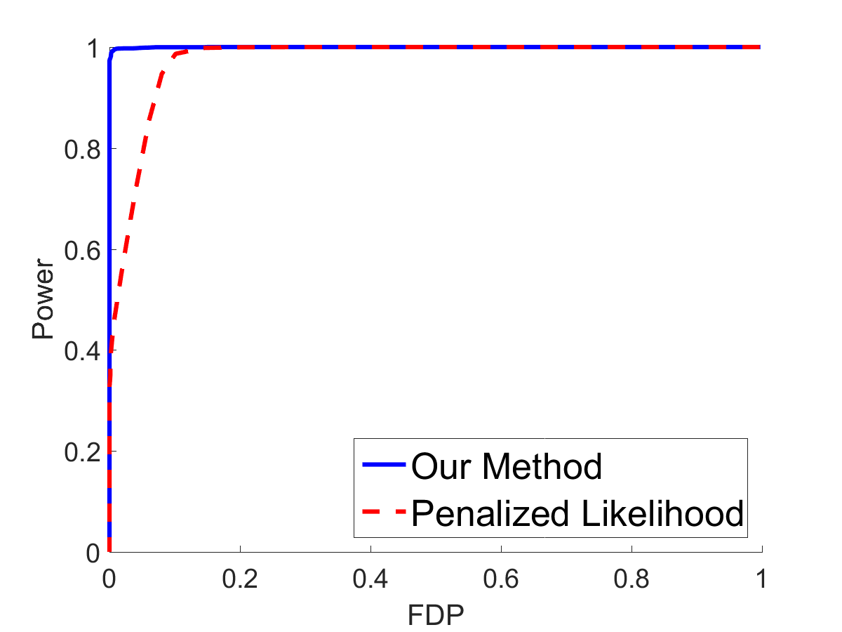
(b) $f=2$

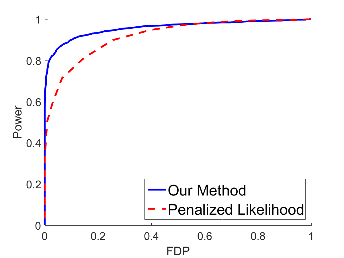
(c) $f=3$

Figure 1: ROC curves for different signal strength when $\boldsymbol{\Omega}$ and $\boldsymbol{\Gamma}$ are bandable matrices.

In this study, we present comparisons between our method and the penalized likelihood approach in Leng and Tang (2012) (with the SCAD penalty) in terms of the ROC curve. We construct the precision matrices $\boldsymbol{\Omega}$ and $\boldsymbol{\Gamma}$ using the graph structures in Section 5.1 but introducing an additional factor $f$ to tune the signal strength. In particular, for hub graph, we set $\boldsymbol{\Omega}_{1}=(\omega_{ij})$ with $\omega_{ij}=\omega_{ji}=0.5/f$; for band graph, we set $\omega_{i,i+1}=\omega_{i+1,i}=0.6/f$ and $\omega_{i,i+2}=\omega_{i+2,i}=0.3/f$; and for random graph, we choose $u_{ij}\sim U(0.4/f,0.8/f)$. When $f=1$, the construction of $\boldsymbol{\Omega}$ and $\boldsymbol{\Gamma}$ is the same as that in Section 5.1. The higher the value of $f$ is, the weaker the signal strength is. Due to space constraints, we only report the comparison when $n=20$, $p=q=100$ and observations are similar for other settings of $n,p,$ and $q$.

We first compare the support recovery performance for different signal strengths by varying $f=1,2,3$ and fix $\boldsymbol{\Omega}$ and $\boldsymbol{\Gamma}$ to be bandable matrices. We note that the usual ROC curve for binary classification is based on false positive rate (a.k.a. $1-$ specificity) vs true positive rate (a.k.a. sensitivity or power). However, our problem is essentially a highly unbalanced classification and thus the standard ROC curve is not suitable. In other words, in our high-dimensional setting, $\boldsymbol{\Omega}\otimes\boldsymbol{\Gamma}$ is a highly sparse matrix and thus the false positive rate will be extremely small for any reasonable choice of $\alpha$ or regularization parameter that give a small number of discoveries. Therefore, we choose to report the ROC curve in terms of FDP vs power, from which, one can easily compare powers for different methods under the same level of FDP. As one can see from Figure 1, our method achieves better performance than the method in Leng and Tang (2012) for different signal strengths. When the factor $f=3$, the ROC curve of our method is still almost vertical. In Section 5.6 in the supplement, we fix the factor $f=3$ and consider different types of $\boldsymbol{\Omega}$ and $\boldsymbol{\Gamma}$. For most cases, our method still achieves better performance.

Real data analysis

For the real data analysis, we investigate the performance of the proposed method on two real datasets, the U.S. agricultural export data from Leng and Tang (2012) and the climatological data from Lozano et al. (2009). Due to space constraints, the details of real data analysis are provided in Section 5.7 in the supplement.

Discussions and future work

In this paper, we propose new test statistics with FDR control guarantees for graph estimation from matrix-variate Gaussian data. To handle the correlation structure among “row samples” and “column samples”, we develop the variance correlation technique. The proposed variance correlation technique can be directly extended to address the problem of learning high-dimensional GGMs with correlated samples, which has not been studied in the existing literature but finds many important applications in practice. We leave this extension as a future work.

To establish the FDR control result, the correlation among “row samples” makes the theoretical analysis significantly more challenging than the i.i.d. case and all the analysis in the i.i.d. case must be carefully tailored. For example, we need to establish the consistency for Lasso estimators from correlated samples. We also need a few new large deviation bounds on sample covariance matrices with correlated samples (see Section 1 in the supplement).

There are several future directions of this work. First, although our paper mainly focuses on the support recovery and graph estimation, it is also interesting to estimate the Kronecker product precision matrix based on the multiple testing framework. Moreover, our work relies on the the Kronecker product structure, it is interesting to consider other forms of the covariance matrices, e.g., the true covariance matrix does not exactly follow Kronecker product structure but close to that structure.

Supplementary Materials

The supplementary material consists of several technical lemmas and the proofs of our propositions and theorems. Moreover, it includes additional simulation studies and real data analysis.

Acknowledgements

The authors are very grateful to two anonymous referees and the associate editor for their detailed and constructive comments that considerably improved the quality of this paper. We would also like to thank Yichen Zhang for helpful discussions and Chenlei Leng and Cheng Yong Tang for sharing the code of Leng and Tang (2012) and U.S. export data. Weidong Liu’s research is supported by NSFC, Grants No. 11322107 and No. 11431006, the Program for Professor of Special Appointment (Eastern Scholar) at Shanghai Institutions of Higher Learning, Shanghai Shuguang Program, Shanghai Youth Talent Support Program and 973 Program (2015CB856004).

Supplementary Material

Technical Lemmas

We introduce several technical lemmas, which will be used throughout the proofs of our propositions and theorems. In particular, let $\boldsymbol{\Psi}=(\psi_{ij})_{q\times q}$ and recall the definition of $\widehat{\boldsymbol{\Psi}}=(\widehat{\psi}_{ij})_{q\times q}$ from Section 3.2. We first prove a maximal concentration inequality on $\widehat{\psi}_{ij}$ in Lemma 1. Note that this result differs from the standard concentration inequality on the sample covariance matrix with i.i.d. samples since the “row samples” for constructing $\widehat{\boldsymbol{\Psi}}$ are correlated.

Lemma 1.

We have for any $M>0$, there exists a constant $C$ such that

$$\mathbb{P}\Big{(}\max_{1\leq i\leq j\leq q}\Big{|}\widehat{\psi}_{ij}-\frac{\mathrm{tr}(\boldsymbol{\Sigma})}{p}\psi_{ij}\Big{|}\geq C\sqrt{\frac{\log\max(q,np)}{np}}\Big{)}=O((q+np)^{-M}).$$

Proof. Recall that for any pair of $i\in[q]$ and $j\in[q]$

$$\widehat{\psi}_{ij} = \frac{1}{(n-1)p}\sum_{k=1}^{n}\sum_{l=1}^{p}(X^{(k)}_{li}-\bar{X}_{li})(X^{(k)}_{lj}-\bar{X}_{lj})$$ (1.35)

$$= \frac{1}{(n-1)p}\sum_{l=1}^{p}\sum_{k=1}^{n}(X^{(k)}_{li}-\bar{X}_{li})(X^{(k)}_{lj}-\bar{X}_{lj}),\$$

where $\bar{X}_{li}=\frac{1}{n}\sum_{k=1}^{n}X^{(k)}_{li}$ and $\bar{X}_{lj}=\frac{1}{n}\sum_{k=1}^{n}X^{(k)}_{lj}$. Without loss of generality, we assume that $\boldsymbol{\mu}=0$.

Let $\textbf{A}\in\text{R}^{n\times n}$ be an orthogonal matrix with the last row $(\frac{1}{\sqrt{n}},\ldots,\frac{1}{\sqrt{n}})$. Let $\mathbf{Y}_{li}=(Y^{(1)}_{li},\ldots,Y^{(n)}_{li})^{{}^{\prime}}=\textbf{A}(X^{(1)}_{li},\ldots,X^{(n)}_{li})^{{}^{\prime}}\in\mathbb{R}^{n\times 1}$. So we have $\sqrt{n}\bar{X}_{li}=Y^{(n)}_{li}$ and

$$\sum_{k=1}^{n}(X^{(k)}_{li}-\bar{X}_{li})(X^{(k)}_{lj}-\bar{X}_{lj})=\mathbf{Y}_{li}^{{}^{\prime}}\mathbf{Y}_{lj}-Y^{(n)}_{li}Y^{(n)}_{lj}=\sum_{k=1}^{n-1}Y^{(k)}_{li}Y^{(k)}_{lj}.$$ (1.36)

Since $(X^{(1)}_{li},\ldots,X^{(n)}_{li})^{{}^{\prime}}\sim N(\mathbf{0},\sigma_{ll}\psi_{ii}\mathbf{I}_{n\times n})$, $(Y^{(1)}_{li},\ldots,Y^{(n-1)}_{li})^{{}^{\prime}}\sim N(\mathbf{0},\sigma_{ll}\psi_{ii}\mathbf{I}_{(n-1)\times(n-1)})$. Let $\textbf{Y}_{k}=(Y^{(k)}_{li})_{1\leq l\leq p,1\leq i\leq q}$ for $1\leq k\leq n-1$. We have $\textbf{Y}_{k}\sim N(\mathbf{0},\boldsymbol{\Sigma}\otimes\boldsymbol{\Psi})$ and $\textbf{Y}_{k}$, $1\leq k\leq n-1$, are independent. Let us define $\mathbf{Z}_{k}=\boldsymbol{\Sigma}^{-1/2}\mathbf{Y}_{k}\sim N(\mathbf{0},\mathbf{I}_{p\times p}\otimes\boldsymbol{\Psi})$. Let $\mathbf{Z}_{ki}$ be the $i$-th column of $\mathbf{Y}_{k}$. Then $(\textbf{Z}_{ki},\textbf{Z}_{kj})\sim N(0,\mathbf{I}_{p\times p}\otimes\boldsymbol{\Psi}_{[i,j]})$, where $\boldsymbol{\Psi}_{[i,j]}=\left(\begin{array}[]{cc}\varphi_{ii}&\varphi_{ij}\\ \varphi_{ji}&\varphi_{jj}\\ \end{array}\right).$

Let the $\textbf{U}^{{}^{\prime}}\textbf{D}\textbf{U}$ be the eigenvalue decomposition of $\boldsymbol{\Sigma}$, where U is an orthogonal matrix and $\textbf{D}={\mathrm{diag}}(\lambda^{(1)}_{1},\ldots,\lambda^{(1)}_{p})$. Define $(\textbf{W}_{ki},\textbf{W}_{kj}):=(\textbf{U}\textbf{Z}_{ki},\textbf{U}\textbf{Z}_{kj})\in\mathbb{R}^{p\times 2}$ where $\textbf{W}_{ki}=(w_{ki,1},\ldots,w_{ki,p})^{{}^{\prime}}\in\mathbb{R}^{p\times 1}$ and $\textbf{W}_{kj}=(w_{kj,1},\ldots,w_{kj,p})^{{}^{\prime}}\in\mathbb{R}^{p\times 1}$. Since $\mathbf{U}$ is an orthogonal matrix, $(\textbf{W}_{ki},\textbf{W}_{kj})\sim N(\mathbf{0},\mathbf{I}_{p\times p}\otimes\boldsymbol{\Psi}_{[i,j]})$, which also implies that $(w_{ki,l},w_{kj,l})$ are independent for $1\leq l\leq p$.

Now combining (1.35) and (1.36), we have,

$$\widehat{\psi}_{ij} = \frac{1}{(n-1)p}\sum_{l=1}^{p}\sum_{k=1}^{n-1}\mathbf{Y}_{ki}^{\prime}\mathbf{Y}_{ki}$$ (1.37)

$$= \frac{1}{(n-1)p}\sum_{k=1}^{n-1}(\textbf{U}\textbf{Z}_{ki})^{{}^{\prime}}\textbf{D}\textbf{U}\textbf{Z}_{kj}$$ (1.38)

$$= \frac{1}{(n-1)p}\sum_{k=1}^{n-1}\sum_{l=1}^{p}\lambda^{(1)}_{l}w_{ki,l}w_{kj,l}.$$ (1.39)

We further note that

$$\mathbb{E}\widehat{\psi}_{ij}=\frac{1}{(n-1)p}\sum_{k=1}^{n-1}\sum_{l=1}^{p}\lambda^{(1)}_{l}\psi_{ij}=\frac{\mathrm{tr}(\boldsymbol{\Sigma})}{p}\psi_{ij}.$$

Put $w_{kij,l}=w_{ki,l}w_{kj,l}-\mathbb{E}w_{ki,l}w_{kj,l}$. We have for some $\eta>0$ such that $\mathbb{E}e^{2\eta|\lambda^{(1)}_{l}w_{kij,l}|}\leq K$ for some $K>0$, uniformly in $i,j,l,k$. It implies that

$$\sum_{k=1}^{n-1}\sum_{l=1}^{p}\mathbb{E}(\lambda^{(1)}_{l}w_{kij,l})^{2}e^{\eta|\lambda^{(1)}_{l}w_{kij,l}|} \leq K\sum_{k=1}^{n-1}\sum_{l=1}^{p}(\mathbb{E}(\lambda^{(1)}_{l}w_{kij,l})^{4})^{1/2}$$

$$= \sqrt{2}K(n-1)\|\boldsymbol{\Sigma}\|^{2}_{F}(\varphi_{ii}\varphi_{jj}+\varphi^{2}_{ij}).$$

By the exponential inequality in Lemma 1 in Cai and Liu (2011) and $\|\boldsymbol{\Sigma}\|^{2}_{F}/p\leq\lambda^{(1)}_{p}$, for any $M>0$, there exists a constant $C>0$,

$$\mathbb{P}\Big{(}|\widehat{\psi}_{ij}-\mathbb{E}\widehat{\psi}_{ij}|\geq C\sqrt{\frac{\log\max(q,np)}{np}}\Big{)}=O((q+np)^{-M}).$$

This proves Lemma 1. ∎

The next concentration inequality involves the residuals. In particular, for $k\in[n]$, $l\in[p]$ and $j\in[q]$, we define:

$$\widetilde{\varepsilon}^{(k)}_{lj}=\varepsilon^{(k)}_{lj}-\frac{1}{n}\sum_{k=1}^{n}\varepsilon^{(k)}_{lj}=:\varepsilon^{(k)}_{lj}-\bar{\varepsilon}_{lj},\quad\widehat{\sigma}_{jj,\varepsilon}=\frac{1}{(n-1)p}\sum_{k=1}^{n}\sum_{l=1}^{p}\left(\widetilde{\varepsilon}^{(k)}_{lj}\right)^{2}.$$

Lemma 2.

For any $M>0$, there exists a constant $C$ such that

$$\mathbb{P}\Big{(}\max_{1\leq i\leq q}\max_{1\leq h\leq q,h\neq i}\Big{|}\frac{1}{np}\sum_{k=1}^{n}\sum_{l=1}^{p}\widetilde{\varepsilon}^{(k)}_{li}(X^{(k)}_{lh}-\bar{X}_{lh})\Big{|}\geq C\sqrt{\frac{\log\max(q,np)}{np}}\Big{)}=O((q+np)^{-M})$$

and

$$\mathbb{P}\Big{(}\max_{1\leq i\leq p}\Big{|}\frac{1}{np}\sum_{k=1}^{n}\sum_{l=1}^{p}\widetilde{\varepsilon}^{(k)}_{li}(\textbf{X}^{(k)}_{l,-i}-\bar{\textbf{X}}_{l,-i})\boldsymbol{\beta}_{i}\Big{|}\geq C\sqrt{\frac{\log\max(q,np)}{np}}\Big{)}=O((q+np)^{-M}).$$

Proof. Recall that

$$\varepsilon^{(k)}_{li}=X^{(k)}_{li}-\alpha_{li}-\textbf{X}^{(k)}_{l,-i}\boldsymbol{\beta}_{i}.$$

Set $\boldsymbol{\varepsilon}^{(k)}_{i}=(\varepsilon^{(k)}_{1i},\ldots,\varepsilon^{(k)}_{pi})^{{}^{\prime}}$ and $\mathbf{Y}^{(k)}_{i}=(\textbf{X}^{(k)}_{1,-i}\boldsymbol{\beta}_{i},\ldots,\textbf{X}^{(k)}_{p,-i}\boldsymbol{\beta}_{i})^{{}^{\prime}}$. It is easy to see that $\mathrm{Cov}(\boldsymbol{\varepsilon}^{(k)}_{i})=\gamma_{ii}^{-1}\boldsymbol{\Sigma}$. Let $\textbf{X}^{(k)}_{h}$ be the $h$-th column of $\textbf{X}^{(k)}$. Since $\boldsymbol{\varepsilon}^{(k)}_{i}$ and $\textbf{X}^{(k)}_{h}$ are independent for $h\neq i$, for the $p\times 2$ matrix $(\boldsymbol{\varepsilon}^{(k)}_{i},\textbf{X}^{(k)}_{h})$, we have $\mathrm{Cov}((\boldsymbol{\varepsilon}^{(k)}_{i},\textbf{X}^{(k)}_{h}))=\boldsymbol{\Sigma}\otimes{\mathrm{diag}}(\gamma_{ii}^{-1},\psi_{ii})$ for $h\neq i$.

In addition, $\mathbf{X}^{(k)}_{\cdot,-i}\sim N(\mathbf{0},\boldsymbol{\Sigma}\otimes\boldsymbol{\Psi}_{-i,-i})$ and $\boldsymbol{\beta}_{i}=-\frac{1}{\gamma_{ii}}\boldsymbol{\Gamma}_{-i,i}$, we have

$$\mathrm{Cov}(\mathbf{Y}^{(k)}_{i})=\frac{1}{\gamma_{ii}^{2}}\mathrm{tr}(\boldsymbol{\Gamma}_{-i,i}\boldsymbol{\Gamma}_{i,-i}\boldsymbol{\Psi}_{-i,-i})\boldsymbol{\Sigma}.$$

Further, by the fact that,

$$\mathrm{tr}(\boldsymbol{\Gamma}_{-i,i}\boldsymbol{\Gamma}_{i,-i}\boldsymbol{\Psi}_{-i,-i})=\boldsymbol{\Gamma}_{i,-i}\boldsymbol{\Psi}_{-i,-i}\boldsymbol{\Gamma}_{-i,i}=-\gamma_{ii}\boldsymbol{\Psi}_{i,-i}\boldsymbol{\Gamma}_{-i,i}=-\gamma_{ii}(1-\psi_{ii}\gamma_{ii}),$$

which further implies that,

$$\mathrm{Cov}(\mathbf{Y}^{(k)}_{i})=\frac{\psi_{ii}\gamma_{ii}-1}{\gamma_{ii}}\boldsymbol{\Sigma}.$$

Since $\boldsymbol{\varepsilon}^{(k)}_{i}$ and $\mathbf{Y}^{(k)}_{i}$ are independent, $\mathrm{Cov}((\boldsymbol{\varepsilon}^{(k)}_{i},\mathbf{Y}^{(k)}_{i}))=\boldsymbol{\Sigma}\otimes{\mathrm{diag}}(\gamma_{ii}^{-1},(\psi_{ii}\gamma_{ii}-1)/\gamma_{ii})$. Following exactly the same proof of Lemma 1, where we replace $(X^{(k)}_{li},X^{(k)}_{lj})$ by $(\varepsilon^{(k)}_{li},X^{(k)}_{lh})$ or $(\varepsilon^{(k)}_{li},\textbf{X}^{(k)}_{l,-i}\boldsymbol{\beta}_{i})$ and $\boldsymbol{\Psi}_{[i,j]}$ by ${\mathrm{diag}}(\gamma_{ii}^{-1},\psi_{ii})$ or ${\mathrm{diag}}(\gamma_{ii}^{-1},(\psi_{ii}\gamma_{ii}-1)/\gamma_{ii})$, we can obtain Lemma 2 immediately. ∎

Lemma 3.

(i). We have, as $np\rightarrow\infty$,

$$\frac{\sum_{k=1}^{n}\sum_{l=1}^{p}(\widetilde{\varepsilon}^{(k)}_{li}\widetilde{\varepsilon}^{(k)}_{lj}-\mathbb{E}\widetilde{\varepsilon}^{(k)}_{li}\widetilde{\varepsilon}^{(k)}_{lj})}{\sqrt{n_{1}\|\boldsymbol{\Sigma}\|^{2}_{F}}}\rightarrow N\Big{(}0,\frac{1}{\gamma_{ii}\gamma_{jj}}+\frac{\gamma^{2}_{ij}}{(\gamma_{ii}\gamma_{jj})^{2}}\Big{)}$$

in distribution.

(ii). For any $M>0$, there exists a constant $C$ such that

$$\mathbb{P}\Big{(}\max_{1\leq i\leq j\leq q}\Big{|}\widehat{\sigma}_{ij,\varepsilon}-\frac{\mathrm{tr}(\boldsymbol{\Sigma})}{p}\frac{\gamma_{ij}}{\gamma_{ii}\gamma_{jj}}\Big{|}\geq C\sqrt{\frac{\log\max(q,np)}{np}}\Big{)}=O((q+np)^{-M}).$$

Proof. Note that $\mathrm{Cov}(\varepsilon^{(k)}_{li},\varepsilon^{(k)}_{li})=\frac{\gamma_{ij}}{\gamma_{ii}\gamma_{jj}}$. It is easy to show that $\mathrm{Cov}((\boldsymbol{\varepsilon}^{(k)}_{i},\boldsymbol{\varepsilon}^{(k)}_{j}))=\boldsymbol{\Sigma}\otimes\Delta_{[i,j]}$, where $\Delta_{[i,j]}=\left(\begin{array}[]{cc}\frac{1}{\gamma_{ii}}&\frac{\gamma_{ij}}{\gamma_{ii}\gamma_{jj}}\\ \frac{\gamma_{ji}}{\gamma_{ii}\gamma_{jj}}&\frac{1}{\gamma_{jj}}\\ \end{array}\right).$ As in the proof of Lemma 1, we can write

$$\sum_{k=1}^{n}\sum_{l=1}^{p}\widetilde{\varepsilon}^{(k)}_{li}\widetilde{\varepsilon}^{(k)}_{lj} = \sum_{k=1}^{n-1}\sum_{l=1}^{p}\lambda^{(1)}_{l}\eta_{ki,l}\eta_{kj,l},$$ (1.40)

where $(\eta_{ki,l},\eta_{kj,l})$, $1\leq l\leq p$, $1\leq k\leq n-1$, are i.i.d. $N(0,\Delta_{[i,j]})$ random vectors. Note that $\mathrm{Var}(\eta_{ki,l}\eta_{kj,l})=\frac{1}{\gamma_{ii}\gamma_{jj}}+\frac{\gamma^{2}_{ij}}{(\gamma_{ii}\gamma_{jj})^{2}}$ and $\sum_{l=1}^{p}(\lambda^{(1)}_{l})^{2}=\|\boldsymbol{\Sigma}\|^{2}_{\text{F}}$. (i) follows from Lindeberg-Feller central limit theorem. (ii) follows from the exponential inequality in Lemma 1 in Cai and Liu (2011). ∎

Proof of Proposition 1–3 on the properties of the proposed test statistics

Proof of Proposition 1. For notational simplicity, let $n_{1}=n-1$ and $\zeta^{(k)}_{lji}=\widetilde{\varepsilon}^{(k)}_{lj}+(X_{li}-\bar{X}_{li})\beta_{i,j}$. Note that for all $k\in[n]$ and $i\neq j$,

$$\widehat{\varepsilon}^{(k)}_{lji}=\widetilde{\varepsilon}^{(k)}_{lj}+(X_{li}-\bar{X}_{li})\beta_{i,j}-(\textbf{X}^{(k)}_{l,-j}-\bar{\textbf{X}}_{l,-j})(\widehat{\boldsymbol{\beta}}_{j,\setminus i}-\boldsymbol{\beta}_{j,\setminus i}),$$

which implies that

$$\widehat{\varepsilon}^{(k)}_{lij}\widehat{\varepsilon}^{(k)}_{lji} = \zeta^{(k)}_{lij}\zeta^{(k)}_{lji}-\zeta^{(k)}_{lij}(\textbf{X}^{(k)}_{l,-j}-\bar{\textbf{X}}_{l,-j})(\widehat{\boldsymbol{\beta}}_{j,\setminus i}-\boldsymbol{\beta}_{j,\setminus i})$$ (2.43)

$$-\zeta^{(k)}_{lji}(\textbf{X}^{(k)}_{l,-i}-\bar{\textbf{X}}_{l,-i})(\widehat{\boldsymbol{\beta}}_{i,\setminus j}-\boldsymbol{\beta}_{i,\setminus j})$$

$$+(\widehat{\boldsymbol{\beta}}_{i,\setminus j}-\boldsymbol{\beta}_{i,\setminus j})^{{}^{\prime}}(\textbf{X}^{(k)}_{l,-i}-\bar{\textbf{X}}_{l,-i})^{{}^{\prime}}(\textbf{X}^{(k)}_{l,-j}-\bar{\textbf{X}}_{l,-j})(\widehat{\boldsymbol{\beta}}_{j,\setminus i}-\boldsymbol{\beta}_{j,\setminus i}).$$

Let $\sigma=\mathrm{tr}(\boldsymbol{\Sigma})/p$. By the assumption (C1), we have $c^{-1}\leq\sigma\leq c$. For the last term in (2.43), by Cauchy-Schwarz inequality, we have

$$\left|\frac{1}{n_{1}p}\sum_{k=1}^{n}\sum_{l=1}^{p}(\widehat{\boldsymbol{\beta}}_{i,\setminus j}-\boldsymbol{\beta}_{i,\setminus j})^{{}^{\prime}}(\textbf{X}^{(k)}_{l,-i}-\bar{\textbf{X}}_{l,-i})^{{}^{\prime}}(\textbf{X}^{(k)}_{l,-j}-\bar{\textbf{X}}_{l,-j})(\widehat{\boldsymbol{\beta}}_{j,\setminus i}-\boldsymbol{\beta}_{j,\setminus i})\ \right|$$

$$\leq \max_{1\leq i,j\leq p}\left|(\widehat{\boldsymbol{\beta}}_{i,\setminus j}-\boldsymbol{\beta}_{i,\setminus j})^{{}^{\prime}}\widehat{\boldsymbol{\Psi}}_{-i,-i}(\widehat{\boldsymbol{\beta}}_{i,\setminus j}-\boldsymbol{\beta}_{i,\setminus j})\right|.$$

For any $i,j\in[q]$, we have

$$|(\widehat{\boldsymbol{\beta}}_{i,\setminus j}-\boldsymbol{\beta}_{i,\setminus j})^{{}^{\prime}}\widehat{\boldsymbol{\Psi}}_{-i,-i}(\widehat{\boldsymbol{\beta}}_{i,\setminus j}-\boldsymbol{\beta}_{i,\setminus j})| \leq |(\widehat{\boldsymbol{\beta}}_{i,\setminus j}-\boldsymbol{\beta}_{i,\setminus j})^{{}^{\prime}}(\widehat{\boldsymbol{\Psi}}_{-i,-i}-\sigma\boldsymbol{\Psi}_{-i,-i})(\widehat{\boldsymbol{\beta}}_{i,\setminus j}-\boldsymbol{\beta}_{i,\setminus j})|$$

$$+\sigma|(\widehat{\boldsymbol{\beta}}_{i,\setminus j}-\boldsymbol{\beta}_{i,\setminus j})^{{}^{\prime}}\boldsymbol{\Psi}_{-i,-i}(\widehat{\boldsymbol{\beta}}_{i,\setminus j}-\boldsymbol{\beta}_{i,\setminus j})|.$$

By Lemma 1,

$$\max_{1\leq i,j\leq q}|(\widehat{\boldsymbol{\beta}}_{i,\setminus j}-\boldsymbol{\beta}_{i,\setminus j})^{{}^{\prime}}(\widehat{\boldsymbol{\Psi}}_{-i,-i}-\sigma\boldsymbol{\Psi}_{-i,-i})(\widehat{\boldsymbol{\beta}}_{i,\setminus j}-\boldsymbol{\beta}_{i,\setminus j})|=O_{\mathbb{P}}\Big{(}a^{2}_{n1}\sqrt{\frac{\log\max(q,np)}{np}}\Big{)}.$$

Moreover,

$$|(\widehat{\boldsymbol{\beta}}_{i,\setminus j}-\boldsymbol{\beta}_{i,\setminus j})^{{}^{\prime}}\boldsymbol{\Psi}_{-i,-i}(\widehat{\boldsymbol{\beta}}_{i,\setminus j}-\boldsymbol{\beta}_{i,\setminus j})|=O_{\mathbb{P}}(\lambda_{\max}(\boldsymbol{\Psi})|\widehat{\boldsymbol{\beta}}_{i}-\boldsymbol{\beta}_{i}|_{2}^{2})$$

uniformly in $i\in[q]$. Combining the above arguments,

$$\left|\frac{1}{n_{1}p}\sum_{k=1}^{n}\sum_{l=1}^{p}(\widehat{\boldsymbol{\beta}}_{i,\setminus j}-\boldsymbol{\beta}_{i,\setminus j})^{{}^{\prime}}(\textbf{X}^{(k)}_{l,-i}-\bar{\textbf{X}}_{l,-i})^{{}^{\prime}}(\textbf{X}^{(k)}_{l,-j}-\bar{\textbf{X}}_{l,-j})(\widehat{\boldsymbol{\beta}}_{j,\setminus i}-\boldsymbol{\beta}_{j,\setminus i})\ \right|$$ (2.44)

$$\quad=O_{\mathbb{P}}\Big{(}a_{n2}^{2}+a^{2}_{n1}\sqrt{\frac{\log\max(q,np)}{np}}\Big{)}.$$ (2.45)

Under the null $H_{0ij}:\gamma_{ij}=0$, we have $\zeta^{(k)}_{lji}=\widetilde{\varepsilon}^{(k)}_{lj}$. Note that

$$(\textbf{X}^{(k)}_{l,-j}-\bar{\textbf{X}}_{l,-j})(\widehat{\boldsymbol{\beta}}_{j,\setminus i}-\boldsymbol{\beta}_{j,\setminus i})=(\textbf{X}^{(k)}_{l,-\{i,j\}}-\bar{\textbf{X}}_{l,-\{i,j\}})(\widehat{\boldsymbol{\beta}}_{j,-i}-\boldsymbol{\beta}_{j,-i}).$$ (2.46)

So

$$\zeta^{(k)}_{lij}(\textbf{X}^{(k)}_{l,-j}-\bar{\textbf{X}}_{l,-j})(\widehat{\boldsymbol{\beta}}_{j,\setminus i}-\boldsymbol{\beta}_{j,\setminus i}) = \sum_{h\neq i,j}\widetilde{\varepsilon}^{(k)}_{li}(X^{(k)}_{lh}-\bar{X}_{lh})(\widehat{\beta}_{h,j}-\beta_{h,j}),$$

where $\widehat{\boldsymbol{\beta}}_{j}=(\widehat{\beta}_{1,j},\ldots,\widehat{\beta}_{p-1,j})^{{}^{\prime}}$ and we set $\widehat{\beta}_{p,j}=0$. By Lemma 2 (i),

$$\max_{1\leq i\leq j\leq q}\Big{|}\sum_{h\neq i,j}\frac{1}{n_{1}p}\sum_{k=1}^{n}\sum_{l=1}^{p}\widetilde{\varepsilon}^{(k)}_{li}(X^{(k)}_{lh}-\bar{X}_{lh})(\widehat{\beta}_{h,j}-\beta_{h,j})\Big{|}$$ (2.47)

$$\leq \max_{1\leq i\leq j\leq q}\max_{h\neq i,j}\left|\frac{1}{n_{1}p}\sum_{k=1}^{n}\sum_{l=1}^{p}\widetilde{\varepsilon}^{(k)}_{li}(X^{(k)}_{lh}-\bar{X}_{lh})\right||\widehat{\boldsymbol{\beta}}_{j}-\boldsymbol{\beta}_{j}|_{1}$$ (2.48)

$$= O_{\mathbb{P}}\Big{(}a_{n1}\sqrt{\frac{\log\max(q,np)}{np}}\Big{)}.$$ (2.49)

A similar inequality holds for the third term on the right hand side of (2.43). Therefore, for $i\neq j$, under $\gamma_{ij}=0$,

$$\frac{1}{n_{1}p}\sum_{k=1}^{n}\sum_{l=1}^{p}\widehat{\varepsilon}^{(k)}_{lij}\widehat{\varepsilon}^{(k)}_{lji} = \frac{1}{n_{1}p}\sum_{k=1}^{n}\sum_{l=1}^{p}\widetilde{\varepsilon}^{(k)}_{li}\widetilde{\varepsilon}^{(k)}_{lj}$$ (2.51)

$$+O_{\mathbb{P}}\Big{(}(a^{2}_{n1}+a_{n1})\sqrt{\frac{\log\max(q,np)}{np}}+a_{n2}^{2}\Big{)}$$

uniformly in $1\leq i\neq j\leq q$. By (2.44) and (2.47) with $i=j$, we obtain that

$$\widehat{r}_{ii}=\frac{1}{n_{1}p}\sum_{k=1}^{n}\sum_{l=1}^{p}(\widetilde{\varepsilon}^{(k)}_{li})^{2}+O_{\mathbb{P}}\Big{(}(a^{2}_{n1}+a_{n1})\sqrt{\frac{\log\max(q,np)}{np}}+a_{n2}^{2}\Big{)}$$ (2.52)

uniformly in $1\leq i\leq q$. The proof of Proposition 1 is complete by Lemma 3. ∎

Proof of Proposition 2. By Lemma 1, it is easy to show that

$$\frac{1}{n_{1}p}\sum_{k=1}^{n}\sum_{l=1}^{p}(X_{li}-\bar{X}_{li})(\textbf{X}^{(k)}_{l,-i}-\bar{\textbf{X}}_{l,-i})(\widehat{\boldsymbol{\beta}}_{i,\setminus j}-\boldsymbol{\beta}_{i,\setminus j})=O_{\mathbb{P}}(a_{n1})$$ (2.53)

uniformly in $i,j$. Also, by (2.46) and (2.47),

$$\frac{1}{n_{1}p}\sum_{k=1}^{n}\sum_{l=1}^{p}\widetilde{\varepsilon}^{(k)}_{li}(\textbf{X}^{(k)}_{l,-j}-\bar{\textbf{X}}_{l,-j})(\widehat{\boldsymbol{\beta}}_{j,\setminus i}-\boldsymbol{\beta}_{j,\setminus i})=O_{\mathbb{P}}\Big{(}a_{n1}\sqrt{\frac{\log\max(q,np)}{np}}\Big{)}.$$ (2.54)

By (2.44), (2.52), (2.53) and (2.54), it suffices to prove that

$$\frac{p}{\mathrm{tr}(\boldsymbol{\Sigma})}\frac{\sqrt{\gamma_{ii}\gamma_{jj}}}{n_{1}p}\sum_{k=1}^{n}\sum_{l=1}^{p}\zeta^{(k)}_{lij}\zeta^{(k)}_{lji}-(1-\gamma_{ij}\psi_{ij})\rho^{\boldsymbol{\Gamma}}_{ij\cdot}\rightarrow 0$$ (2.55)

in probability. We have

$$\mathbb{E}\Big{[}(\varepsilon^{(k)}_{lj}+X_{li}\beta_{i,j})(\varepsilon^{(k)}_{li}+X_{lj}\beta_{i,j})\Big{]}=\sigma_{ll}(-\frac{\gamma_{ij}}{\gamma_{ii}\gamma_{jj}}+\psi_{ij}\frac{\gamma^{2}_{ij}}{\gamma_{ii}\gamma_{jj}}).$$

Now, as the proof of Lemma 1, we can write

$$\sum_{k=1}^{n}\sum_{l=1}^{p}\zeta^{(k)}_{lij}\zeta^{(k)}_{lji}=\sum_{k=1}^{n-1}\sum_{l=1}^{p}\lambda^{(1)}_{l}\xi_{ki,l}\xi_{kj,l},$$ (2.56)

where $(\xi_{ki,l},\xi_{kj,l})$, $1\leq l\leq p$, are i.i.d. with $\mathbb{E}\xi_{ki,l}\xi_{kj,l}=(-\frac{\gamma_{ij}}{\gamma_{ii}\gamma_{jj}}+\psi_{ij}\frac{\gamma^{2}_{ij}}{\gamma_{ii}\gamma_{jj}})$. This proves (2.55). ∎

Proof of Proposition 3. Let $\phi_{ij}=\frac{\mathrm{tr}(\boldsymbol{\Gamma})}{q}\sigma_{ij}$ and define $\widetilde{\lambda}=\lambda\sqrt{\frac{\log\max(p,nq)}{nq}}$. We have

$$\sum_{j=1}^{p}\widehat{\sigma}^{2}_{ij,\lambda}=\sum_{j=1}^{p}(\widehat{\sigma}^{2}_{ij}-\phi^{2}_{ij})I\{|\widehat{\sigma}_{ij}|\geq\widetilde{\lambda}\}+\sum_{j=1}^{p}\phi^{2}_{ij}I\{|\widehat{\sigma}_{ij}|\geq\widetilde{\lambda}\}.$$

Also by Lemma 1, with probability tending to one,

$$\sum_{j=1}^{p}\phi^{2}_{ij}I\{|\widehat{\sigma}_{ij}|<\widetilde{\lambda}\}\leq\sum_{j=1}^{p}\phi^{2}_{ij}I\{|\phi_{ij}|<2\widetilde{\lambda}\}=O(\widetilde{\lambda}^{2-\tau}s(p))$$

uniformly in $1\leq i\leq p$ by the assumption (C2). So, for the last term,

$$\sum_{j=1}^{p}\phi^{2}_{ij}I\{|\widehat{\sigma}_{ij}|\geq\widetilde{\lambda}\}=\sum_{j=1}^{p}\phi^{2}_{ij}-\sum_{j=1}^{p}\phi^{2}_{ij}I\{|\widehat{\sigma}_{ij}|<\widetilde{\lambda}\}=(1+O_{\mathbb{P}}(\widetilde{\lambda}^{2-\tau}s(p)))\sum_{j=1}^{p}\phi^{2}_{ij}$$

uniformly in $1\leq i\leq p$. Moreover, with probability tending to one,

$$\sum_{j=1}^{p}|\widehat{\sigma}^{2}_{ij}-\phi^{2}_{ij}|I\{|\widehat{\sigma}_{ij}|\geq\widetilde{\lambda}\} = \sum_{j=1}^{p}|\widehat{\sigma}_{ij}+\phi_{ij}||\widehat{\sigma}_{ij}-\phi_{ij}|I\{|\widehat{\sigma}_{ij}|\geq\widetilde{\lambda}\}$$

$$\leq C\sum_{j=1}^{p}|\phi_{ij}||\widehat{\sigma}_{ij}-\phi_{ij}|I\{|\phi_{ij}|\geq\widetilde{\lambda}/2\}$$

$$\leq C\widetilde{\lambda}^{-(\tau-1)\vee 0}\sum_{j=1}^{p}|\phi_{ij}|^{\tau}|\widehat{\sigma}_{ij}-\phi_{ij}|$$

$$\leq C\widetilde{\lambda}^{(2-\tau)\wedge 1}s(p),$$

where the last inequality following from $\max_{1\leq i\leq j\leq q}|\widehat{\sigma}_{ij}-\phi_{ij}|=O_{\mathbb{P}}(\widetilde{\lambda})$ by Lemma 1. It implies that $\max_{1\leq i\leq q}|\sum_{j=1}^{p}\widehat{\sigma}^{2}_{ij,\lambda}-\sum_{j=1}^{p}\phi^{2}_{ij}|=O_{\mathbb{P}}(\widetilde{\lambda}^{(2-\tau)\wedge 1}s(p))$ and hence

$$\frac{\|\widehat{\boldsymbol{\Sigma}}_{\lambda}\|^{2}_{F}}{\|\boldsymbol{\Sigma}\|^{2}_{F}}=O_{\mathbb{P}}(\widetilde{\lambda}^{(2-\tau)\wedge 1}s(p)).$$

By Lemma 1, we have $\mathrm{tr}(\widehat{\boldsymbol{\Sigma}}_{\lambda})/\mathrm{tr}(\boldsymbol{\Sigma})=O_{\mathbb{P}}(\widetilde{\lambda})$. This implies this proposition holds. ∎

Proof of Theorems 1–4 on FDR control and power analysis

It is easy to see that the Benjamini and Hochberg (BH) method is equivalent to reject $H_{0ij}$ if $|\widehat{T}_{ij}|\geq\widehat{t}$, where

$$\widehat{t}=\inf\Big{\{}t\geq 0:\frac{G(t)(q^{2}-q)/2}{\max\{\sum_{1\leq i<j\leq q}I\{|\widehat{T}_{ij}|\geq t\},1\}}\leq\alpha\Big{\}},$$ (3.57)

where $G(t):=2-2\Phi(t)$. We first give some key lemmas which are the generalization of Lemmas 6,1 and 6.2 in Liu (2013) from i.i.d. case to independent case (but not necessarily identically distributed).

Let $\xi_{1},\ldots,\xi_{n}$ be independent $d$-dimensional random vectors with mean zero. Define $|\cdot|_{(d)}$ by $|\mathbf{z}|_{(d)}=\min\{|z_{i}|;1\leq i\leq d\}$ for $\mathbf{z}=(z_{1},\ldots,z_{d})^{{}^{\prime}}$. Let $(p,n)$ be a sequence of positive integers and the constants $c,r,b,\gamma,K,C$ mentioned below do not depend on $(p,n)$.

Lemma 4.

Suppose that $p\leq cn^{r}$ and $\max_{1\leq k\leq n}\mathbb{E}|\xi_{k}|_{2}^{bdr+2+\epsilon}\leq K$ for some fixed $c>0$, $r>0$, $b>0$, $K>0$ and $\epsilon>0$. Assume that $\|\frac{1}{n}\mathrm{Cov}(\sum_{k=1}^{n}\xi_{k})-\mathbf{I}_{d}\|\leq C(\log p)^{-2-\gamma}$ for some $\gamma>0$ and $C>0$. Then we have

$$\sup_{0\leq t\leq\sqrt{b\log p}}\Big{|}\frac{\mathbb{P}(|\sum_{k=1}^{n}\xi_{k}|_{(d)}\geq t\sqrt{n})}{(G(t))^{d}}-1\Big{|}\leq C(\log p)^{-1-\gamma_{1}}$$

for $\gamma_{1}=\min\{\gamma,1/2\}$.

Let $\boldsymbol{\eta}_{k}=(\eta_{k1},\eta_{k2})^{{}^{\prime}}$, $1\leq k\leq n$, are independent $2$-dimensional random vectors with mean zero.

Lemma 5.

Suppose that $p\leq cn^{r}$ and $\max_{1\leq k\leq n}\mathbb{E}|\boldsymbol{\eta}_{k}|_{2}^{2br+2+\epsilon}<\infty$ for some fixed $c>0$, $r>0$, $b>0$ and $\epsilon>0$. Assume that $\sum_{k=1}^{n}\mathrm{Var}(\eta_{k1})=\sum_{k=1}^{n}\mathrm{Var}(\eta_{k2})=n$ and $|\frac{1}{n}\sum_{k=1}^{n}\mathrm{Cov}(\eta_{k1},\eta_{k2})|\leq\delta$ for some $0\leq\delta<1$. Then we have

$$\mathbb{P}\Big{(}|\sum_{k=1}^{n}\eta_{k1}|\geq t\sqrt{n},|\sum_{k=1}^{n}\eta_{k2}|\geq t\sqrt{n}\Big{)}\leq C(t+1)^{-2}\exp(-t^{2}/(1+\delta))$$

uniformly for $0\leq t\leq\sqrt{b\log p}$, where $C$ only depends on $c,b,r,\epsilon,\delta$.

The proofs of Lemmas 4 and 5 are the same as those of Lemma 6.1 and 6.2 in Liu (2013).

Recall $\eta_{ki,l}$ in (1.40) and $\xi_{ki,l}$ in (2.56). For $1\leq i<j\leq q$, let

$$U_{ij}=\frac{\sum_{k=1}^{n-1}\sum_{l=1}^{p}\lambda^{(1)}_{l}(\eta_{ki,l}\eta_{kj,l}-\mathbb{E}\eta_{ki,l}\eta_{kj,l})(\gamma_{ii}\gamma_{jj})^{1/2}}{\sqrt{(n-1)pE_{p}}},$$ (3.58)

$$V_{ij}=\frac{\sum_{k=1}^{n-1}\sum_{l=1}^{p}\lambda^{(1)}_{l}(\xi_{ki,l}\xi_{kj,l}-\mathbb{E}\xi_{ki,l}\xi_{kj,l})(\gamma_{ii}\gamma_{jj})^{1/2}}{\sqrt{(n-1)pE_{p}}},$$ (3.59)

where $E_{p}=p^{-1}\sum_{l=1}^{p}(\lambda^{(1)}_{l})^{2}$. Note that $\lambda^{(1)}_{l}$ are bounded away from zero and infinity. Also, $\mathrm{Var}(\eta_{ki,l}\eta_{kj,l})=(\gamma_{ii}\gamma_{jj})^{-1}(1+\gamma^{2}_{ij}(\gamma_{ii}\gamma_{jj})^{-1})$, $\mathrm{Var}(U_{ij})=1+\gamma^{2}_{ij}(\gamma_{ii}\gamma_{jj})^{-1}$ and $Corr(U_{ij},U_{kl})=Corr(\eta_{1i,1}\eta_{1j,1},\eta_{1k,1}\eta_{1l,1})$. By Lemma 4 with $d=1$, we have

$$\max_{1\leq i,j\leq q}\sup_{0\leq t\leq 4\sqrt{\log q}}\Big{|}\frac{\mathbb{P}(|U_{ij}|\geq t\sqrt{1+\gamma^{2}_{ij}(\gamma_{ii}\gamma_{jj})^{-1}})}{G(t)}-1\Big{|}\leq C(\log q)^{-1-\epsilon},$$

$$\max_{1\leq i,j\leq q}\sup_{0\leq t\leq 4\sqrt{\log q}}\Big{|}\frac{\mathbb{P}(|V_{ij}|\geq t\sqrt{\mathrm{Var}(\xi_{1i,1}\xi_{1j,1})\gamma_{ii}\gamma_{jj}})}{G(t)}-1\Big{|}\leq C(\log q)^{-1-\epsilon},$$

for some $\epsilon>0$. Therefore, $\max_{1\leq i,j\leq q}|U_{ij}|=O_{\mathbb{P}}(\sqrt{\log q})$ and $\max_{1\leq i,j\leq q}|V_{ij}|=O_{\mathbb{P}}(\sqrt{\log q})$. This, together with (2.52), Lemma 3, Proposition 3, the proof of Proposition 2, (4.27) and (2.51), implies that

$$\max_{1\leq i<j\leq q}\Big{|}\widehat{T}_{ij}+b_{nij}\sqrt{\frac{(n-1)p}{A_{p}}}(1-\gamma_{ij}\psi_{ij})\rho^{\boldsymbol{\Gamma}}_{ij\cdot}-V_{ij}\Big{|}=o_{\mathbb{P}}((\log q)^{-1/2})$$ (3.60)

as $np,q\rightarrow\infty$, where $b_{nij}$ satisfies $\max_{1\leq i<j\leq q}|b_{nij}-1|\rightarrow 0$ in probability. Note that under the null $\gamma_{ij}=0$, $U_{ij}=V_{ij}$. Now Theorem 1 follows from the proof of Theorem 3.1 in Liu (2013) step by step, by using Lemmas 4 and 5 and replacing $U_{ij}$ in Liu (2013) by $U_{ij}$ in (3.58) and the sample size in Liu (2013) by $(n-1)p$. The proof of Theorem 2 is similar. Theorem 3 follows from the formula of FDP and Theorems 1 and 2.

Under (4.33), we have $\mathrm{Var}(\xi_{1i,1}\xi_{1j,1})\gamma_{ii}\gamma_{jj}=1+o(1)$ uniformly in $i,j$. Hence $\max_{1\leq i<j\leq q}|V_{ij}|\leq(2+\delta)\sqrt{\log q}$ for some $\delta>0$ with probability tending to one. This shows that

$$\mathbb{P}\Big{(}\min_{(i,j)\in\mathcal{H}_{1}}|\widehat{T}_{ij}|\geq(2+\delta^{{}^{\prime}})\sqrt{\log q}\Big{)}\rightarrow 1.$$

for some $\delta^{{}^{\prime}}>0$. By the definition of $\widehat{t}$ in (3.57), we have $\widehat{t}\leq 2\sqrt{\log q}$ as $q\rightarrow\infty$. Thus, $\mathbb{P}(\mathcal{H}_{1}\subseteq\widehat{\text{supp}(\boldsymbol{\Gamma})})\rightarrow 1$. Similarly, we can show that $\mathbb{P}(\mathcal{H}^{{}^{\prime}}_{1}\subseteq\widehat{\text{supp}(\boldsymbol{\Omega})})\rightarrow 1$. This finishes the proof of Theorem 4.∎

Proof of Proposition 4 on the convergence rate of $\widehat{\boldsymbol{\beta}}_{j}$

Proof of Proposition 4. Define

$$\widehat{\mathbf{a}}_{j}=\frac{1}{(n-1)p}\sum_{k=1}^{n}\sum_{l=1}^{p}(\textbf{X}^{(k)}_{l,-j}-\bar{\textbf{X}}_{l,-j})^{{}^{\prime}}(X^{(k)}_{lj}-\bar{X}_{lj}).$$

We let $\theta_{nj}$ and $\boldsymbol{\alpha}_{j}$ denote $\theta_{nj}(\delta)=\delta\sqrt{\frac{\widehat{\psi}_{jj}\log q}{np}}$ and $\boldsymbol{\alpha}_{j}(\delta)$ (defined in (3.18)), respectively. By the Karush-Kuhn-Tucker (KKT) condition, we have

$$\Big{|}\textbf{D}^{-1/2}_{j}\widehat{\boldsymbol{\Psi}}_{-j,-j}\widehat{\boldsymbol{\beta}}_{j}-\textbf{D}^{-1/2}_{j}\widehat{\mathbf{a}}_{j}\Big{|}_{\infty}\leq\theta_{nj}.$$ (4.61)

By Lemma 1, we have $c^{-1}\leq\min_{1\leq j\leq q-1}\mathbf{D}_{j}\leq\max_{1\leq j\leq q-1}\mathbf{D}_{j}\leq c$ for some $c>0$ with probability tending to one. This, together with Lemma 2, implies that, for sufficiently large $\delta$,

$$\Big{|}\frac{1}{(n-1)p}\textbf{D}^{-1/2}_{j}\sum_{k=1}^{n}\sum_{l=1}^{p}(\textbf{X}^{(k)}_{l,-j}-\bar{\textbf{X}}_{l,-j})^{{}^{\prime}}\widetilde{\varepsilon}^{(k)}_{lj}\Big{|}_{\infty}\leq\frac{1}{2}\theta_{nj}$$ (4.62)

uniformly in $1\leq j\leq q$, with probability tending to one. Note that $\widetilde{\varepsilon}^{(k)}_{lj}=X^{(k)}_{lj}-\bar{X}_{lj}-(\textbf{X}^{(k)}_{l,-j}-\bar{\textbf{X}}_{l,-j})\boldsymbol{\beta}_{j}.$ Therefore,

$$\Big{|}\textbf{D}^{-1/2}_{j}\widehat{\boldsymbol{\Psi}}_{-j,-j}\boldsymbol{\beta}_{j}-\textbf{D}^{-1/2}_{j}\widehat{\mathbf{a}}_{j}\Big{|}_{\infty}\leq\frac{1}{2}\theta_{nj}$$ (4.63)

uniformly in $1\leq j\leq q$. Note that inequalities (4.61) and (4.63) imply that

$$\Big{|}\textbf{D}^{-1/2}_{j}\widehat{\boldsymbol{\Psi}}_{-j,-j}(\widehat{\boldsymbol{\beta}}_{j}-\boldsymbol{\beta}_{j})\Big{|}_{\infty}\leq\frac{3}{2}\theta_{nj}.$$ (4.64)

Define $\boldsymbol{\Lambda}={\mathrm{diag}}(\boldsymbol{\Psi})^{-1/2}\boldsymbol{\Psi}{\mathrm{diag}}(\boldsymbol{\Psi})^{-1/2}$. For any subset $T\subset\{1,2,\cdots,q-1\}$ and $\boldsymbol{\nu}\in\mathbb{R}^{q-1}$ with $|T|=o\Big{(}\sqrt{\frac{np}{\log\max(q,np)}}\Big{)}$ and $|\boldsymbol{\nu}_{T^{c}}|_{1}\leq c|\boldsymbol{\nu}_{T}|_{1}$ for some $c>0$, by Lemma 1 and the conditions in Proposition 4, we have

$$\boldsymbol{\nu}^{{}^{\prime}}\textbf{D}^{-1/2}_{j}\widehat{\boldsymbol{\Psi}}_{-j,-j}\textbf{D}^{-1/2}_{j}\boldsymbol{\nu}\geq\lambda_{\min}(\boldsymbol{\Lambda}_{-j,-j})|\boldsymbol{\nu}|_{2}^{2}-O_{\mathbb{P}}\Big{(}\sqrt{\frac{\log\max(q,np)}{np}}\Big{)}|\boldsymbol{\nu}|^{2}_{1}\geq|\boldsymbol{\nu}|_{2}^{2}/C,$$ (4.65)

for some constant $C>0$, where the first inequality follows from the fact

$$|\boldsymbol{\nu}^{{}^{\prime}}(\textbf{D}^{-1/2}_{j}\widehat{\boldsymbol{\Psi}}_{-j,-j}\textbf{D}^{-1/2}_{j}-\boldsymbol{\Lambda}_{-j,-j})\boldsymbol{\nu}|\leq|\textbf{D}^{-1/2}_{j}\widehat{\boldsymbol{\Psi}}_{-j,-j}\textbf{D}^{-1/2}_{j}-\boldsymbol{\Lambda}_{-j,-j}|_{\infty}|\boldsymbol{\nu}|^{2}_{1}$$

and the second inequality follows from the fact $|\boldsymbol{\nu}|^{2}_{1}\leq(1+c)^{2}|\boldsymbol{\nu}_{T}|^{2}_{1}\leq(1+c)^{2}|T||\boldsymbol{\nu}|^{2}_{2}$.

Now let $T$ be the support of $\boldsymbol{\beta}_{j}$, $\boldsymbol{\alpha}_{j}=\mathbf{D}_{j}^{1/2}\boldsymbol{\beta}_{j}$ and $\boldsymbol{\nu}=\mathbf{D}^{1/2}_{j}(\widehat{\boldsymbol{\beta}}_{j}-\boldsymbol{\beta}_{j})=\widehat{\boldsymbol{\alpha}}_{j}-\boldsymbol{\alpha}_{j}$. We first show that $|\boldsymbol{\nu}_{T^{c}}|_{1}\leq 3|\boldsymbol{\nu}_{T}|_{1}$ uniformly in $1\leq j\leq q$ with probability tending to one. Define

$$Q(\boldsymbol{\alpha}_{j}) = \frac{1}{2(n-1)p}\sum_{k=1}^{n}\sum_{l=1}^{p}(X^{(k)}_{lj}-\bar{X}_{lj}-(\textbf{X}^{(k)}_{l,-j}-\bar{\textbf{X}}_{l,-j})\mathbf{D}_{j}^{-1/2}\boldsymbol{\alpha}_{j})^{2},$$

$$S(\boldsymbol{\alpha}_{j}) = \textbf{D}^{-1/2}_{j}\widehat{\mathbf{a}}_{j}-\textbf{D}^{-1/2}_{j}\widehat{\boldsymbol{\Psi}}_{-j,-j}\boldsymbol{\beta}_{j}.$$

Note that $S(\boldsymbol{\alpha}_{j})$ is the gradient of $Q(\boldsymbol{\alpha}_{j})$. By the definition of $\widehat{\boldsymbol{\alpha}}_{j}$, we have

$$Q(\widehat{\boldsymbol{\alpha}}_{j})-Q(\boldsymbol{\alpha}_{j})\leq\theta_{nj}(\delta)|\boldsymbol{\alpha}_{j}|_{1}-\theta_{nj}|\widehat{\boldsymbol{\alpha}}_{j}|_{1}\leq\theta_{nj}(|\boldsymbol{\nu}_{T}|_{1}-|\boldsymbol{\nu}_{T^{c}}|_{1}),$$

and by (4.63), with probability tending to one,

$$Q(\widehat{\boldsymbol{\alpha}}_{j})-Q(\boldsymbol{\alpha}_{j})\geq S^{{}^{\prime}}(\boldsymbol{\alpha}_{j})\boldsymbol{\nu}\geq-\frac{1}{2}\theta_{nj}|\boldsymbol{\nu}|_{1}=-\frac{1}{2}\theta_{nj}(|\boldsymbol{\nu}_{T}|_{1}+|\boldsymbol{\nu}_{T^{c}}|_{1})$$

uniformly in $1\leq j\leq q$. It follows from the above two inequalities that $|\boldsymbol{\nu}_{T^{c}}|_{1}\leq 3|\boldsymbol{\nu}_{T}|_{1}$. So by (4.64) and (4.65) we have

$$|\boldsymbol{\nu}|_{2}^{2} \leq C\boldsymbol{\nu}^{{}^{\prime}}\textbf{D}^{-1/2}_{j}\widehat{\boldsymbol{\Psi}}_{-j,-j}\textbf{D}^{-1/2}_{j}\boldsymbol{\nu}$$

$$\leq C|\textbf{D}^{-1/2}_{j}\widehat{\boldsymbol{\Psi}}_{-j,-j}\textbf{D}^{-1/2}_{j}\boldsymbol{\nu}|_{\infty}|\boldsymbol{\nu}|_{1}$$

$$\leq \frac{3}{2}C\theta_{nj}(|\boldsymbol{\nu}_{T}|_{1}+|\boldsymbol{\nu}_{T^{c}}|_{1})$$

$$\leq 6C\theta_{nj}|\boldsymbol{\nu}_{T}|_{1}$$

$$\leq 6C\theta_{nj}\sqrt{|\boldsymbol{\beta}_{j}|_{0}}|\boldsymbol{\nu}_{T}|_{2}$$

uniformly in $1\leq j\leq q$ with probability tending to one. By noting that $c^{-1}\leq\min_{1\leq j\leq q-1}\mathbf{D}_{j}\leq\max_{1\leq j\leq q-1}\mathbf{D}_{j}\leq c$ with probability tending to one, we have $|\widehat{\boldsymbol{\beta}}_{j}-\boldsymbol{\beta}_{j}|_{2}\leq c|\boldsymbol{\nu}|_{2}$. Hence, by the conditions in Proposition 4, we have $a_{n2}=o_{\mathbb{P}}\Big{(}(np\log q)^{-1/4}\Big{)}$. Note that $|\boldsymbol{\nu}|_{1}\leq 4|\boldsymbol{\nu}_{T}|_{1}\leq 4\sqrt{|\boldsymbol{\beta}_{j}|_{0}}|\boldsymbol{\nu}_{T}|_{2}=o((\log\max(q,np))^{-1})$ uniformly in $1\leq j\leq q-1$ with probability tending to one. This proves Proposition 4 holds. ∎

Additional Experiments

In this section, we present some additional simulation studies and real data analysis. We first note that for the choice of tuning parameters, our theoretical results will hold for any large enough constants $\lambda$ in (3.15) for estimating $\widehat{A}_{p}$ (see Proposition 3) and $\delta>0$ in (3.19) for $\widehat{\boldsymbol{\beta}}_{j}(\delta)$ (see Proposition 4). In our experiment, we will adopt a data-driven parameter-tuning strategy from Liu (2013). In particular, $\lambda$ and $\delta$ are selected by

$$(\widehat{\lambda},\widehat{\delta})=\mathop{\rm arg\min}_{\lambda,\delta}\sum_{k=3}^{9}\left(\frac{\sum_{1\leq i\neq j\leq q}I\{|\widehat{T}_{ij}(\lambda,\delta)|\geq\Phi^{-1}(1-\frac{k}{20})\}}{k(q^{2}-q)/10}-1\right)^{2},$$ (5.66)

where $\widehat{T}_{ij}(\lambda,\delta)$ is the test statistic in (3.14) with an initial estimator $\widehat{\boldsymbol{\beta}}_{j}(\delta)$ and $\widehat{A}_{p}$ (depending on the threshold $\lambda$). The choice of $(\lambda,\delta)$ in (5.66) makes the distributions of $\widehat{T}_{ij}$, on average, close to the standard normal distribution. We note that although the parameter searching is conducted on a two-dimensional grid on $\lambda$ and $\delta$, the main computational cost is the construction of $\widehat{\boldsymbol{\beta}}_{j}(\delta)$, which is irrelevant of $\lambda$. Therefore, the computational cost of the parameter searching is moderate.

Boxplots of FDPs

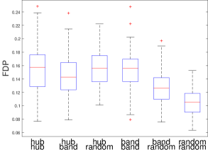
(a) $p=100$, $q=100$

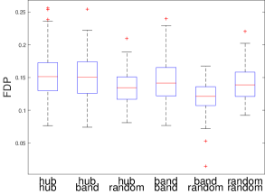
(b) $p=200$, $q=50$

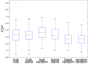
(c) $p=200$, $q=200$

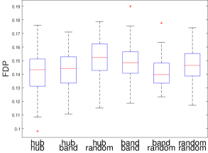
(d) $p=400$, $q=400$

Figure 2: Boxplots for FDP when $n=100$ and $\alpha=0.1$.

We present the boxplots of FDPs when $n=100$ over 100 replications in Figure 2 for different $p$, $q$, and precision matrix structures. As we can see from Figure 2, FDPs are well concentrated, which suggests that the performance of the proposed estimator is quite stable.

Estimation of $\widehat{A}_{p}$

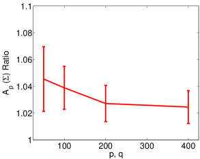
(a) $n=20$

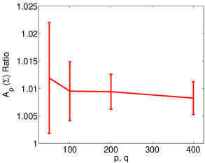
(b) $n=100$

Figure 3: The ratio $\widehat{A}_{p}/A_{p}$ for different $n$ and $p=q$ when $\boldsymbol{\Omega}$ and $\boldsymbol{\Gamma}$ are hub graphs.

In Figure 3, we plot the ratio $\widehat{A}_{p}/A_{p}$ for $n=20$ (left figure) and $n=100$ (right figure) as $p=q$ increases from $50$ to $400$. Due to space constraints, we only show the case when both $\boldsymbol{\Omega}$ and $\boldsymbol{\Gamma}$ are generated from hub graphs (the plots when $\boldsymbol{\Omega}$ and $\boldsymbol{\Gamma}$ are generated from other graphs structures are similar). As one can see from Figure 3, when either $n$ is fixed and $p=q$ increases or $p=q$ is fixed and $n$ increases from 20 to 100, the mean ratio becomes closer to one and the standard deviation of the ratios decreases. This study empirically verifies Proposition 3, which claims that the ratio $\widehat{A}_{p}/A_{p}$ converges to 1 in probability as $nq\rightarrow\infty$.

Comparison to the penalized likelihood approach

Table 2: Averaged empirical FDP and power using the penalized likelihood method with the SCAD penalty.

$p$	$q$	$\boldsymbol{\Omega}$	$\boldsymbol{\Gamma}$	$n=20$		$n=100$
				FDP	Power	FDP	Power
100	100	hub	hub	0.037	0.347	0.038	0.346
		hub	band	0.455	0.410	0.348	0.381
		hub	random	0.722	0.926	0.738	0.910
		band	band	0.341	0.206	0.332	0.167
		band	random	0.339	0.964	0.246	0.971
		random	random	0.703	0.962	0.622	0.943
200	200	hub	hub	0.027	0.322	0.059	0.370
		hub	band	0.357	0.314	0.333	0.306
		hub	random	0.629	0.903	0.654	0.888
		band	band	0.333	0.187	0.333	0.167
		band	random	0.246	0.966	0.151	0.982
		random	random	0.481	0.828	0.326	0.863
200	50	hub	hub	0.060	0.381	0.054	0.385
		hub	band	0.362	0.330	0.371	0.517
		hub	random	0.754	0.927	0.704	0.909
		band	band	0.340	0.205	0.334	0.174
		band	random	0.588	0.833	0.551	0.855
		random	random	0.784	0.961	0.607	0.947
400	400	hub	hub	0.946	0.978	0.952	1.000
		hub	band	0.982	1.000	0.962	0.992
		hub	random	0.949	0.999	0.910	1.000
		band	band	0.338	0.179	0.336	0.175
		band	random	0.233	0.848	0.237	0.864
		random	random	0.141	0.610	0.099	0.644

We compare our procedure with the penalized likelihood approach in Leng and Tang (2012). We adopt the same (regularization) parameter-tuning procedure as Leng and Tang (2012), i.e., we generate an extra random test dataset with the sample size equal to the training set and choose the parameter that maximizes the log-likelihood on the test dataset. Due to space constraints, we only report the result using the SCAD penalty (Fan and Li, 2001) rather than the L1 penalty since the SCAD penalty leads to slightly better performance (also observed in Leng and Tang (2012)). The averaged empirical FDPs and powers for different settings of $n,p,q,\boldsymbol{\Omega},\boldsymbol{\Gamma}$ are shown in Table 2. As one can see from Table 2, each setting has either a large FDP or a small power. In fact, for those settings with small averaged FDPs (e.g., $n=100,p=200,q=50$ and $\boldsymbol{\Omega}$ and $\boldsymbol{\Gamma}$ generated from hub graphs with the averaged FDP 0.054), the corresponding powers are also small (e.g., 0.385 for the aforementioned case), which indicates that the estimated $\widehat{\boldsymbol{\Omega}}$ or $\widehat{\boldsymbol{\Gamma}}$ is too sparse. On the other hand, for those settings with large averaged powers (e.g., $n=100,p=q=400$ and $\boldsymbol{\Omega}$ from hub and $\boldsymbol{\Gamma}$ from random with the averaged power equal to 1), the corresponding FDPs are also large (e.g., 0.910 for the aforementioned case), which indicates that the estimated $\widehat{\boldsymbol{\Omega}}$ or $\widehat{\boldsymbol{\Gamma}}$ is too dense. We also note that when $p,q$ are small as compared to $n$, the penalized likelihood approach still achieves good support recovery performance (e.g., the case $n=100,p=q=20$ as reported in Leng and Tang (2012)). When $p,q$ are comparable to or lager than $n$, our testing based method achieves better support recovery performance.

De-correlation method

In Remark 1, we illustrate why the de-correlation approach is not applicable in our problem setup from a theoretical perspective. Here, we provide some empirical evidences. Due to space constraints, we only report the comparison when $n=20$, $p=q=100$, and, in fact, the performance becomes even worse when $p,q$ gets larger. Ideally, the empirical FDP should be close to (or below) the FDP estimate $\alpha^{\prime}$ in (3.21). However, as one can see from Figure 4, the empirical FDP is much larger than the corresponding $\alpha^{\prime}$ in many cases. Moreover, by setting the FDR level for individual $\boldsymbol{\Gamma}$ and $\boldsymbol{\Omega}$ to be $\alpha=0.1$, we present the corresponding empirical FDP and $\alpha^{\prime}$ in Table 3, where the FDP can be twice as large as $\alpha^{\prime}$ in some cases. The experimental results from Table 3 and Figure 4 empirically verify that the de-correlation approach does not control FDP well.

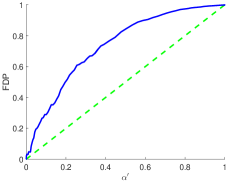
(a) $\boldsymbol{\Omega}=$ hub, $\boldsymbol{\Gamma}=$ hub

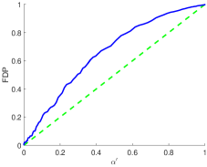
(b) $\boldsymbol{\Omega}=$hub, $\boldsymbol{\Gamma}=$ band

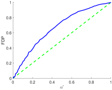
(c) $\boldsymbol{\Omega}=$ hub, $\boldsymbol{\Gamma}=$ random

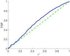
(d) $\boldsymbol{\Omega}=$ band, $\boldsymbol{\Gamma}=$ band

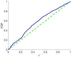
(e) $\boldsymbol{\Omega}=$ band, $\boldsymbol{\Gamma}=$ random

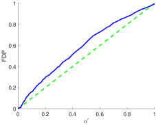
(f) $\boldsymbol{\Omega}=$ random, $\boldsymbol{\Gamma}=$ random

Figure 4: Averaged empirical FDPs (y-axis) against different estimated FDP $\alpha^{\prime}$s (x-axis) for the de-correlation approach. For the purpose of controlling FDP, the blue line should be close to or below the dashed green line, which represents FDP=$\alpha^{\prime}$.

Table 3: Averaged empirical FDP and the estimated FDP $\alpha^{\prime}$ for the de-correlation approach.

$\boldsymbol{\Omega}$	$\boldsymbol{\Gamma}$	FDP	($\alpha^{\prime}$)
hub	hub	0.376	(0.146)
hub	band	0.272	(0.152)
hub	random	0.323	(0.154)
band	band	0.176	(0.161)
band	random	0.199	(0.164)
random	random	0.250	(0.164)

Simulation study when the covariance is not a Kronecker product

In this section, we present simulation study when the covariance matrix does not follow the form of a Kronecker product. More precisely, we generate the covariance matrix in the form of $\boldsymbol{\Sigma}\otimes\boldsymbol{\Psi}+\nu\mathbf{I}$, where $\mathbf{I}$ is the $pq\times pq$ identity matrix and $\nu$ is the level of perturbation. Due to space constraints, we only present the case when $n=20$, $p=q=30$, $\boldsymbol{\Omega}$ is either a band or a hub graph, $\boldsymbol{\Gamma}$ is a random graph. The observation is similar for other settings. Figure 5 plots the ROC curves for different perturbation parameters $\nu=0,0.2,0.5,2$, and $5$. As one can see, when the perturbation level $\nu$ is small, the ROC curve is almost identical to the case when the covariance is a Kronecker product (i.e., $\nu=0$). However, when $\nu$ becomes larger, the support recovery performance becomes inferior.

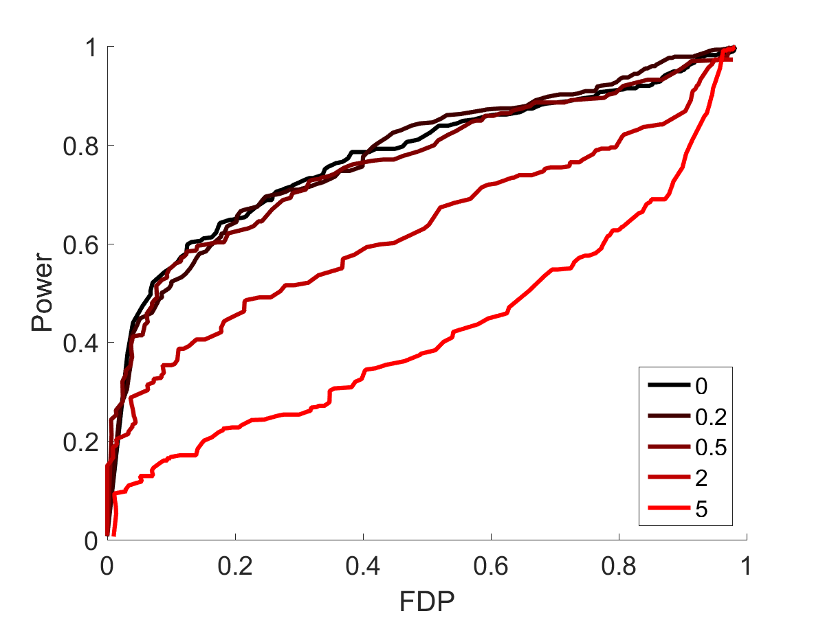
(a) $\boldsymbol{\Omega}=$ band, $\boldsymbol{\Gamma}=$random

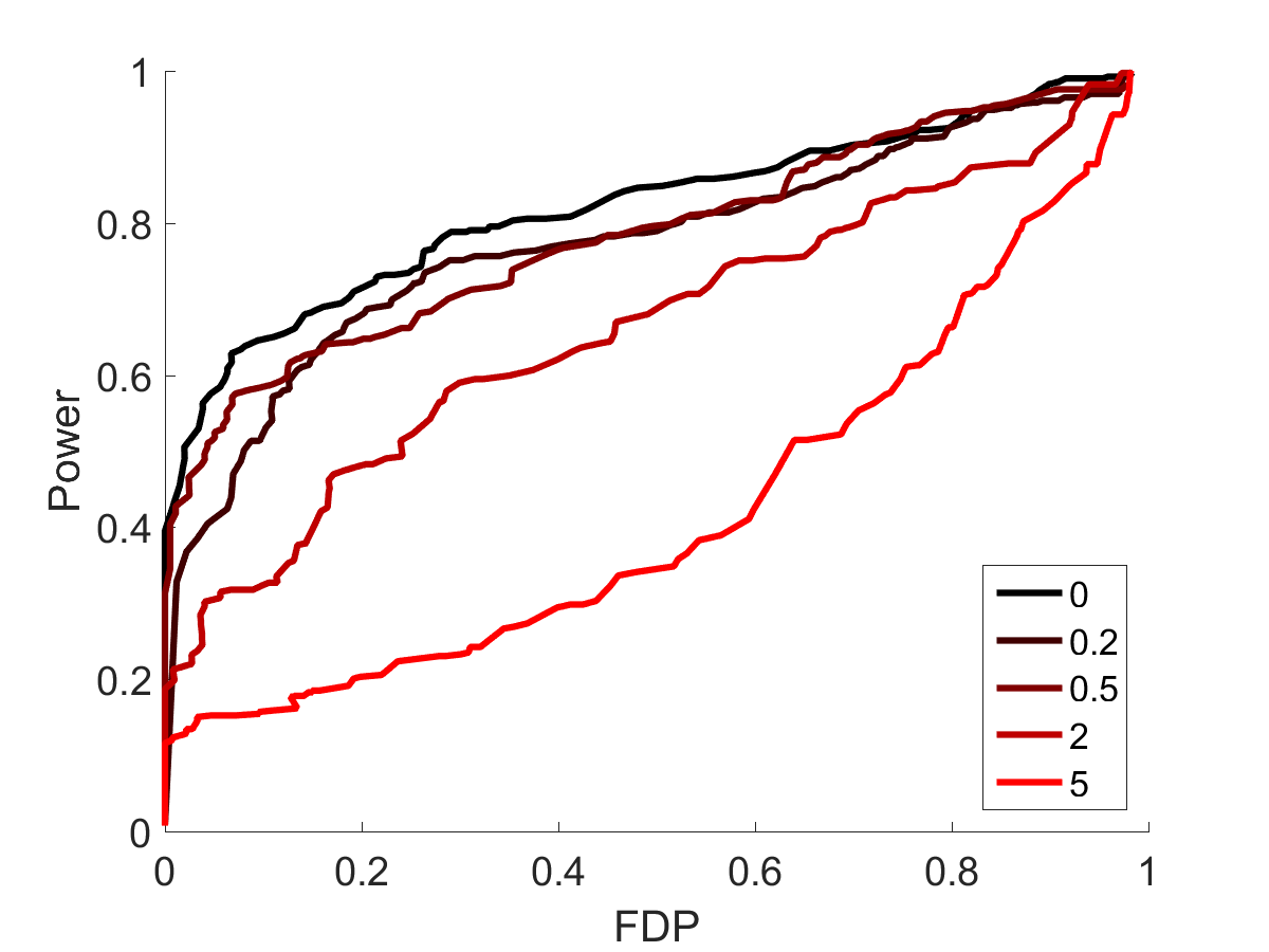
(b) $\boldsymbol{\Omega}=$ hub, $\boldsymbol{\Gamma}=$ random

Figure 5: ROC curves for different perturbation levels of $\nu=0,0.2,0.5,2$ and $5$. The larger the $\nu$ is, the more “red” color of the ROC curve is (from black to red).

Additional ROC curve comparisons

In Figure 6, we fix the factor $f=3$ and consider different types of $\boldsymbol{\Omega}$ and $\boldsymbol{\Gamma}$. For most cases, our method achieves better performance. The only exception is that, for hub/random and band/random graphs, the power of the penalized likelihood approach outperforms our method when FDP is large. However, for support recovery in high-dimensional settings, one is more interested in the scenario when FDP is very small. In such a case, our method consistently leads to a larger power than the penalized likelihood approach.

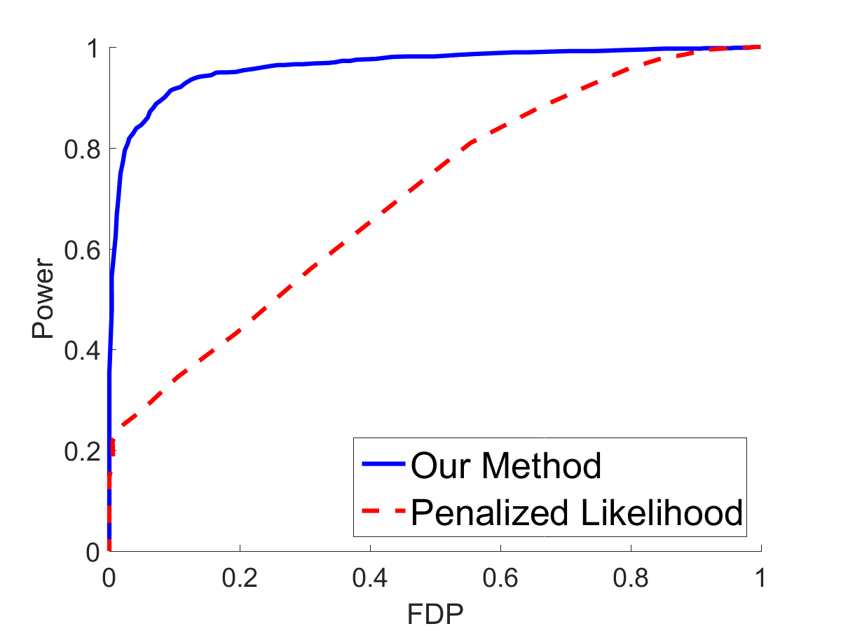
(a) $\boldsymbol{\Omega}=$ hub, $\boldsymbol{\Gamma}=$ hub

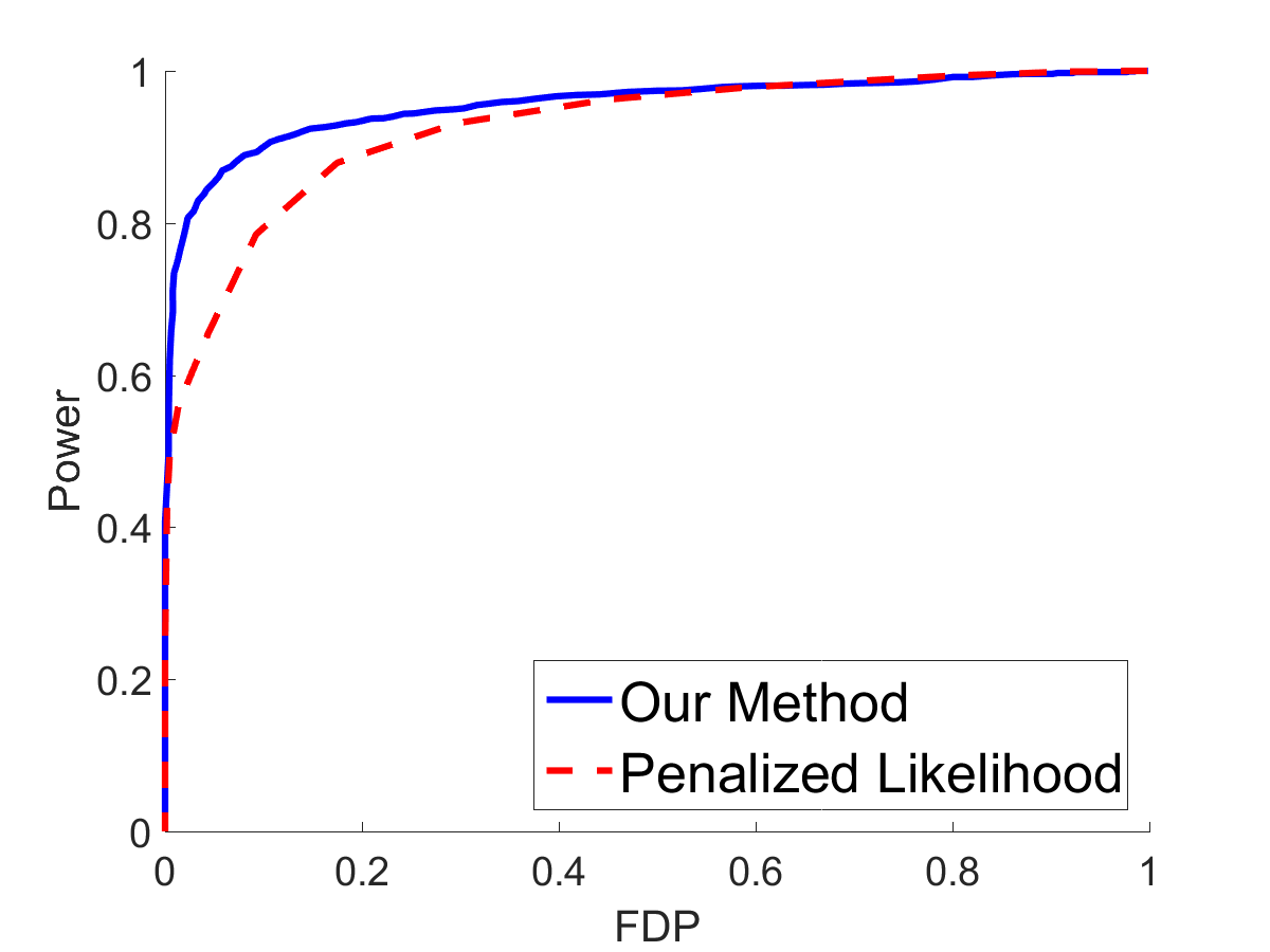
(b) $\boldsymbol{\Omega}=$hub, $\boldsymbol{\Gamma}=$ band

(c) $\boldsymbol{\Omega}=$ hub, $\boldsymbol{\Gamma}=$ random

(d) $\boldsymbol{\Omega}=$ band, $\boldsymbol{\Gamma}=$ band

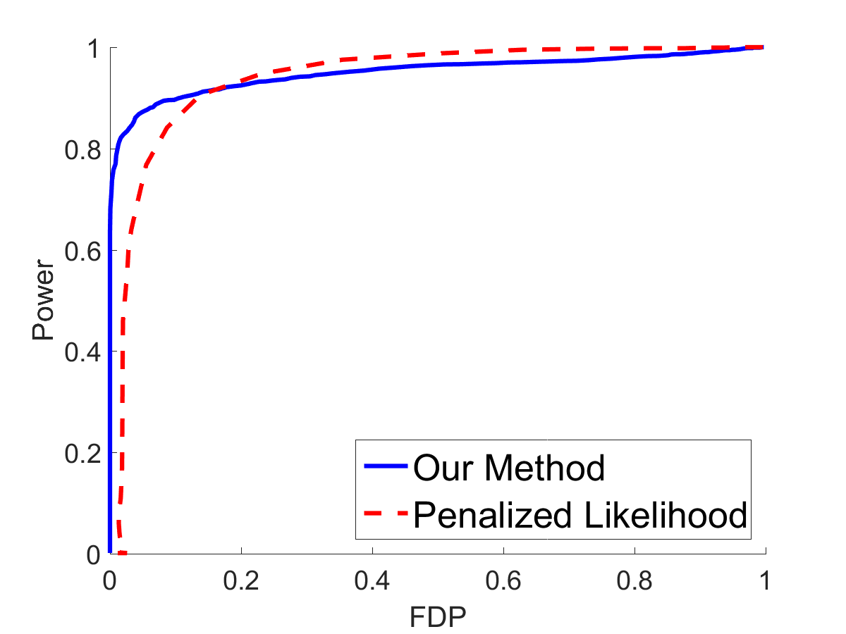
(e) $\boldsymbol{\Omega}=$ band, $\boldsymbol{\Gamma}=$ random

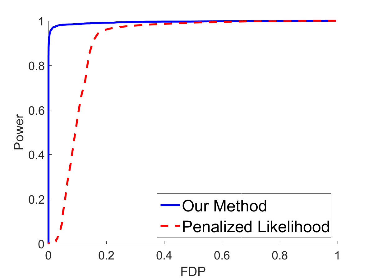
(f) $\boldsymbol{\Omega}=$ random, $\boldsymbol{\Gamma}=$ random

Figure 6: ROC curves for different types of the construction of $\boldsymbol{\Omega}$ and $\boldsymbol{\Gamma}$ when $f=3$.

Real data analysis

In this section, we investigate the performance of the proposed method on two real datasets, the U.S. agricultural export data from Leng and Tang (2012) and the climatological data from Lozano et al. (2009).

U.S. agricultural export data

Table 4: No. of edges for the export data. For 13 regions, there are 78 possible edges in total. For 36 products, there are 630 possible edges in total.

	Region			Product
	$\alpha=0.1$	$\alpha=0.2$	$\alpha=0.3$	$\alpha=0.1$	$\alpha=0.2$	$\alpha=0.3$
No. of Edges	2	23	31	19	30	37
Density of the Graph	2.56%	29.49%	39.74%	3.01%	4.76%	5.87%

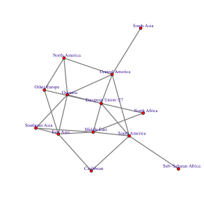
(a) Graph for Regions ($\alpha=0.2$)

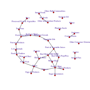
(b) Graph for Products ($\alpha=0.2$)

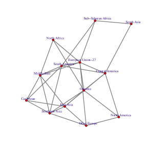
(c) Graph for Regions ($\alpha=0.3$)

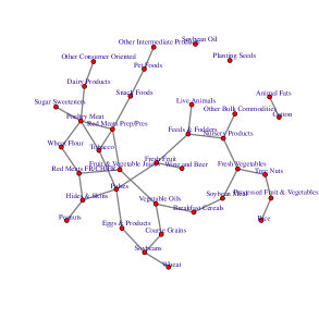
(d) Graph for Products ($\alpha=0.3$)

Figure 7: Estimated graphs for the export data

We first apply our method to the U.S. agricultural export data studied in Leng and Tang (2012). The dataset contains annual U.S. agriculture export data for 40 years, from 1970 to 2009. Each annual dataset contains the amount (in thousands U.S. dollars) of exports for $36$ products (e.g., pet foods, snack foods, breakfast cereals, soybean meal, meats, eggs, dairy products, etc.) in 13 different regions (e.g., North America, Central America, South America, South Asia, etc.). Thus, the dataset can be organized into $40$ matrix-variate observations, where each observation is a $(p=13)\times(q=36)$ matrix. We adopt the method proposed in Leng and Tang (2012) to remove the dependence in this matrix-variate time series data. In particular, we take the logarithm of the original data plus one and then take the lag-one difference for each matrix observation so that the number of observations becomes $n=39$. Please refer to Leng and Tang (2012) for more details on the pre-processing of the data.

We apply the proposed FDR control procedure to estimate the support of the precision matrices for regions and products under different $\alpha\in\{0.1,0.2,0.3\}$. In Table 4, we report the number of edges/discoveries for different $\alpha$’s. We observe that for the product graphs, the number of discoveries is relatively small as compared to the number of hypotheses, which indicates that many pairs of products are conditionally independent. In Figure 7, we plot the graphs corresponding to the estimated supports of $\boldsymbol{\Omega}$ (corresponding to Regions) and $\boldsymbol{\Gamma}$ (corresponding to Products) for $\alpha=0.2$ and $\alpha=0.3$. Figures 7(a) and 7(c) show the estimated graphs for $p=13$ regions. As we can see, the regions in the following sets, $\{\text{East Asia},\;\text{Southeast Asia}\}$, $\{\text{European Union},\;\text{Other Europe},\;\text{Oceania}\}$ and $\{\text{Central America},\;\text{North America},\;\text{South America}\}$, are always connected. Such an observation should be expected since regions in the aforementioned sets are close geographically. This observation is consistent with the result obtained by penalized likelihood approach in Leng and Tang (2012), which claims that “the magnitude between Europe Union and Other Europe, and that between East Asia and Southeast Asia are the strongest.” The regions South Asia, Sub-Saharan Africa, and North Africa connect to fewer regions. This observation is also consistent with the result in Leng and Tang (2012), noting that “interestingly, none of the 11 largest edges corresponds to either North Africa or Sub-Saharan Africa.” The estimated graphs for products shown in Figures 7(b) and 7(d) are quite sparse, which indicates many pairs of products are conditionally independent given the information of the rest of the products. The product graphs also lead to many interesting observations. For example, the products in the following sets, $\{\text{Pet foods},\;\text{Snack foods},\;\text{Other Intermediate Products}\}$,

$\{\text{Dairy Products},\text{Red Meats FR/CH/FR},\text{Red Meats Prep/Pres},\text{Poultry Meat},\text{Wheat Flour}\}$, are always connected (not necessarily directly). Such observations also make sense since different kinds of meats and dairy products are closely related products and thus should be highly correlated.

Climate data analysis

In this section, we study the climatological data from Lozano et al. (2009), which contains monthly data of $p=17$ different meteorological factors during 144 months, from 1990 to 2002. The observations span $q=125$ locations in the U.S. The 17 meteorological factors measured for each month include CO₂, CH₄, H₂, CO, average temperature (TMP), diurnal temperature range (DTR), minimum temperate (TMN), maximum temperature (TMX), precipitation (PRE), vapor (VAP), cloud cover (CLD), wet days (WET), frost days (FRS), global solar radiation (GLO), direct solar radiation (DIR), extraterrestrial radiation (ETR) and extraterrestrial normal radiation (ETRN). We note that we ignore the UV aerosol index factor in Lozano et al. (2009) since most measurements of this factor are missing. We adopt the same procedure as described in Section 5.7.1 to reduce the level of dependence in this matrix-variate time series data.

Table 5: No. of edges for the climate data. For $p=17$ meteorological factors, there are 136 edges in total. For $q=125$ locations, there are 7,750 possible edges in total.

	Meteorological factors			Locations
	$\alpha=0.1$	$\alpha=0.2$	$\alpha=0.3$	$\alpha=0.1$	$\alpha=0.2$	$\alpha=0.3$
No. of Edges	30	40	42	1059	1539	2065
Density of the Graph	22.05%	29.41%	30.88%	13.66%	19.85%	26.65%

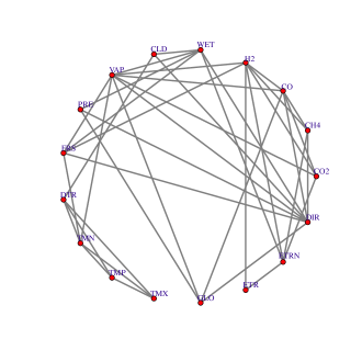
(a) Graph for meteorological factors ($\alpha=0.2$)

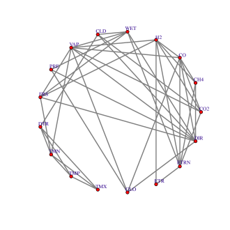
(b) Graph for meteorological factors ($\alpha=0.3$)

Figure 8: Estimated graphs for the climate data

We apply the proposed FDR control procedure to estimate the support of the precision matrices for meteorological factors and locations under different $\alpha\in\{0.1,0.2,0.3\}$. In Table 5, we report the number of edges/discoveries for different $\alpha$’s. From Table 5, the number of discoveries for meteorological factors is quite stable as $\alpha$ increases from 0.1 to 0.3. Moreover, the number of discoveries for locations is relatively large, which indicates many strong correlations among pairs of locations. We plot the graphs corresponding to the estimated supports of the precision matrices for meteorological factors in Figure 8 (the plots for locations are omitted since they are too dense to visualize). An interesting observation is that the factors TMX, TMP, TMN and DTR form a clique. This pattern is reasonable since the factors TMX, TMP, TMN and DTR are all related to temperature and thus should be highly correlated. Other sparsity patterns might also provide insight for understanding dependency relationships among meteorological factors.

Department of Information, Operations & Management Sciences, Stern School of Business, New York University Email: xchen3@stern.nyu.edu

Department of Mathematics, Institute of Natural Sciences and MOE-LSC, Shanghai Jiao Tong University. Email: weidongl@sjtu.edu.cn.

References

- Allen and Tibshirani (2010) Allen, G. I. and Tibshirani, R. (2010) Transposable regularized covariance models with an application to missing data imputation. Annals of Applied Statistics, 4, 764–790.
- Benjamini and Hochberg (1995) Benjamini, Y. and Hochberg, Y. (1995) Controlling the false discovery rate: a practical and powerful approach to multiple testing. Journal of the Royal Statistical Society. Series B (Statistical Methodology), 57, 389–300.
- Bickle and Levina (2008) Bickle, P. and Levina, E. (2008) Regularized estimation of large covariance matrices. Annals of Statistics, 36, 199–227.
- Bijma et al. (2005) Bijma, F., De Munck, J. and Heethaar, R. (2005) The spatiotemporal meg covariance matrix modeled as a sum of kronecker products. NeuroImage, 27, 402–415.
- Bühlmann and van de Geer (2011) Bühlmann, P. and van de Geer, S. (2011) Statistics for High-Dimensional Data — Methods, Theory and Applications. Springer.
- Cai and Liu (2011) Cai, T. and Liu, W. (2011) Adaptive thresholding for sparse covariance matrix estimation. Journal of the American Statistical Association, 106, 672–684.
- Cai et al. (2016) Cai, T., Ren, Z. and Zhou, H. (2016) Estimating structured high-dimensional covariance and precision matrices: Optimal rates and adaptive estimation. Electronic Journal of Statistics, 10, 1–89.
- Cai et al. (2011) Cai, T. T., Liu, W. and Luo, X. (2011) A constrained minimization approach to sparse precision matrix estimation. Journal of the American Statistical Association, 106, 594–607.
- Candès and Tao (2007) Candès, E. and Tao, T. (2007) The dantzig selector: statistical estimation when is much larger than . Annals of Statistics, 35, 2313–2351.
- Chen and Qin (2010) Chen, S. X. and Qin, Y. L. (2010) A two-sample test for high-dimensional data with applications to gene-set testing. Annals of Statistics, 38, 808–835.
- d’Aspremont et al. (2008) d’Aspremont, A., Banerjee, O. and El Ghaoui, L. (2008) First-order methods for sparse covariance selection. SIAM Journal on Matrix Analysis and its Applications, 30, 56–66.
- Dawid (1981) Dawid, A. P. (1981) Some matrix-variate distribution theory: Notational considerations and a bayesian application. Biometrika, 68, 265–274.
- Efron (2009) Efron, B. (2009) Are a set of microarrays independent of each other? Annals of Applied Statistics, 3, 922–942.
- Fan and Li (2001) Fan, J. and Li, R. (2001) Variable selection via nonconcave penalized likelihood and its oracle properties. Journal of the American Statistical Association, 96, 1348–1360.
- Fan and Lv (2016) Fan, Y. and Lv, J. (2016) Innovated scalable efficient estimation in ultra-large gaussian graphical models. Annals of Statistics, 44.
- Friedman et al. (2008) Friedman, J., Hastie, T. and Tibshirani, R. (2008) Sparse inverse covariance estimation with the graphical lasso. Biostatistics, 9, 432–441.
- van de Geer et al. (2014) van de Geer, S., B hlmann, P., Ritov, Y. and Dezeure, R. (2014) On asymptotically optimal confidence regions and tests for high-dimensional models. Annals of Statistics, 42, 1166–1202.
- Gupta and Nagar (1999) Gupta, A. K. and Nagar, D. K. (1999) Matrix Variate Distributions. Chapman Hall.
- Huang and Chen (2015) Huang, F. and Chen, S. (2015) Joint learning of multiple sparse matrix Gaussian graphical models. IEEE Transactions on Neural Networks and Learning Systems, 26, 2606 – 2620.
- Kalaitzis et al. (2013) Kalaitzis, A., Lafferty, J., Lawrence, N. D. and Zhou, S. (2013) The bigraphical lasso. In Proceedings of the 30th International Conference on Machine Learning.
- Lam and Fan (2009) Lam, C. and Fan, J. (2009) Sparsistency and rates of convergence in large covariance matrix estimation. Annals of Statistics, 37, 4254–4278.
- Leng and Tang (2012) Leng, C. and Tang, C. Y. (2012) Sparse matrix graphical models. Journal of the American Statistical Association, 107, 1187–1200.
- Liu et al. (2012) Liu, H., Han, F., Yuan, M., Lafferty, J. and Wasserman, L. (2012) High dimensional semiparametric Gaussian copula graphical models. Annals of Statistics, 40, 2293–2326.
- Liu (2013) Liu, W. (2013) Gaussian graphical model estimation with false discovery rate control. Annals of Statistics, 41, 2948–2978.
- Liu and Shao (2014) Liu, W. and Shao, Q. M. (2014) Phase transition and regularized bootstrap in large-scale -tests with false discovery rate control. Annals of Statistics, 42, 2003–2025.
- Lozano et al. (2009) Lozano, A. C., Li, H., Niculescu-Mizil, A., Liu, Y., Perlich, C., Hosking, J. and Abe, N. (2009) Spatial-temporal causal modeling for climate change attribution. In Proceedings of the 15th ACM SIGKDD International Conference on Knowledge Discovery and Data Mining.
- Ma et al. (2007) Ma, S., Gong, Q. and Bohnert, H. J. (2007) An arabidopsis gene network based on the graphical Gaussian model. Genome Research, 17, 1614–1625.
- Meinshausen and Bühlmann (2006) Meinshausen, N. and Bühlmann, P. (2006) High-dimensional graphs and variable selection with the lasso. Annals of Statistics, 34, 1436–1462.
- Ravikumar et al. (2011) Ravikumar, P., Wainwright, M., Raskutti, G. and Yu, B. (2011) High-dimensional covariance estimation by minimizing -penalized log-determinant divergence. Electronic Journal of Statistics, 5, 935–980.
- Ren et al. (2016) Ren, Z., Kang, Y., Fan, Y. and Lv, J. (2016) Tuning-free heterogeneity pursuit in massive networks. ArXiv preprint arXiv:1606.03803.
- Ren et al. (2015) Ren, Z., Sun, T., Zhang, C. H. and Zhou, H. H. (2015) Asymptotic normality and optimalities in estimation of large Gaussian graphical model. Annals of Statistics, 43, 991–1026.
- Rothman et al. (2008) Rothman, A., Bickel, P., Levina, E. and Zhu, J. (2008) Sparse permutation invariant covariance estimation. Electronic Journal of Statistics, 2, 494–515.
- Schafer and Strimmer (2005) Schafer, J. and Strimmer, K. (2005) An empirical Bayes approach to inferring large-scale gene association networks. Bioinformatics, 21, 754–764.
- Tibshirani (1996) Tibshirani, R. (1996) Regression shrinkage and selection via the lasso. Journal of the Royal Statistical Society. Series B (Statistical Methodology), 58, 267–288.
- Tsiligkaridis et al. (2013) Tsiligkaridis, T., Hero, A. O. and Zhou, S. (2013) Convergence properties of kronecker graphical lasso algorithms. IEEE Transactions on Signal Processing, 61, 1743–1755.
- Xue and Zou (2012) Xue, L. and Zou, H. (2012) Regularized rank-based estimation of high-dimensional nonparanormal graphical models. Annals of Statistics, 40, 2541–2571.
- Yin and Li (2012) Yin, J. and Li, H. (2012) Model selection and estimation in matrix normal graphical model. Journal of Multivariate Analysis, 107, 119–140.
- Ying and Liu (2013) Ying, Y. and Liu, H. (2013) High-dimensional semiparametric bigraphical models. Biometrika, 100, 655–670.
- Yuan (2010) Yuan, M. (2010) Sparse inverse covariance matrix estimation via linear programming. Journal of Machine Learning Research, 11, 2261–2286.
- Yuan and Lin (2007) Yuan, M. and Lin, Y. (2007) Model selection and estimation in the Gaussian graphical model. Biometrika, 94, 19–35.
- Zhou (2014) Zhou, S. (2014) Gemini: Graph estimation with matrix variate normal instances. Annals of Statistics, 42, 532–562.
- Zhu et al. (2014) Zhu, Y., Shen, X. T. and Pan, W. (2014) Structural pursuit over multiple undirected graphs. Journal of the American Statistical Association, 109, 1683–1696.