Gutzwiller Renormalization Group

Abstract

We develop a variational scheme called “Gutzwiller renormalization group” (GRG), which enables us to calculate the ground state of Anderson impurity models (AIM) with arbitrary numerical precision. Our method can exploit the low-entanglement property of the ground state in combination with the framework of the Gutzwiller wavefunction, and suggests that the ground state of the AIM has a very simple structure, which can be represented very accurately in terms of a surprisingly small number of variational parameters. We perform benchmark calculations of the single-band AIM that validate our theory and indicate that the GRG might enable us to study complex systems beyond the reach of the other methods presently available and pave the way to interesting generalizations, e.g., to nonequilibrium transport in nanostructures.

Introduction.— Impurity models are ubiquitous in condensed matter theory. Originally, the AIM was deviced to describe magnetic impurities embedded in metallic hosts and heavy-fermion compound Anderson (1961); Hewson (1997). However, the AIM can be applied to describe many other physical systems, such as quantum dots Madhavan et al. (1998); Cronenwett et al. (1998); van der Wiel et al. (2002) and dissipative two-level systems Vladár and Zawadowski (1983). The importance of impurity models in condensed matter has grown further with the emergence of dynamical mean-field theory (DMFT) Georges et al. (1996) and its success in describing strongly correlated materials Kotliar et al. (2006); Held et al. (2006); Maier et al. (2005); Anisimov and Izyumov (2010). In fact, within DMFT, solving the many-body lattice problem amounts to solve recursively an auxiliary AIM.

Among the many methodologies developed to solve impurity models, one of the most successful is the numerical renormalization group (NRG) Wilson (1975); Hewson (1997), which was originally deviced by Wilson in order to study the Kondo problem, and was based on the idea of “scaling”, previously introduced by Anderson. The starting point of the NRG procedure consists in representing the AIM as a one-dimensional semi-infinite tight-binding linear chain with the impurity situated at one of the boundaries. Within this representation, and by using a logarithmic discretization of the density of states corresponding to exponentially decaying hoppings (Wilson chains), the NRG algorithm consists in a truncation scheme that enables to take into account the coupling between the different length scales progressively, starting from near the impurity (high energies) to longer distances (low energies), while retaining a relatively small number of states at each stage.

More recently, the NRG algorithm has been reinterpreted as a variational method within the framework of the “matrix product states” Saberi et al. (2008); Weichselbaum et al. (2009). From this perspective, the accuracy of NRG can be traced back into the fact that, due to the locality of the interactions within the above mentioned one-dimensional representation of the AIM, the ground state has very low entanglement, and can be consequently accurately represented by a matrix product state with a small bond dimension. Thanks to this interpretation it was also possible to uncover a connection between NRG and the density matrix renormalization group (DMRG) method White (1992, 1993), which can also be formulated as a variational approximation within the framework of the matrix product states Verstraete et al. (2004). Eventually, these ideas resulted in an entirely new class of methods named “variational renormalization group” (VRG) Vaestrate et al. (2008), with broader applications with respect to both NRG and DMRG, encompassing, e.g., systems with dimension higher than 1.

In this work we introduce a variational technique to solve the AIM called “Gutzwiller renormalization group” (GRG), that combines the Gutzwiller variational method Gutzwiller (1963, 1964, 1965) with some of the above mentioned ideas underlying NRG and the other VRG methods. Similarly to the ordinary Gutzwiller theory, the GRG consists in optimizing variationally a wavefunction represented as a Slater determinant extended over the entire system — which is infinite — multiplied by a local operator (named “Gutzwiller projector”), which modifies the corresponding electron configurations. However, in GRG the action of the Gutzwiller projector is not limited only to the correlated impurity. In fact, in analogy with the NRG numerical procedure, in GRG the longer length scales are taken into account with arbitrary accuracy by extending progressively the action of the Gutzwiller projector also to a portion of the one-dimensional bath lying nearby the impurity. Thus, the size of the “projected” region is increased until the desired level of precision is reached.

We perform numerical calculations that demonstrate the quality of the GRG variational ansatz, and present arguments concerning the scaling of the computational complexity of our algorithm indicating that the GRG might enable us to solve AIM beyond the reach of any other presently available technique. Another appealing property of our approach is that it enables us to describe the ground state of the AIM in the thermodynamical limit and at all length scales, while this is technically very difficult with any other existing technique, including NRG, DMRG, and the Bethe ansatz Andrei (1980); Andrei et al. (1983); Weigmann (1980).

The Anderson Impurity Model.— For sake of simplicity, here our approach will be formulated for the single-band AIM represented in Fig. 1, where the correlated impurity is connected to a bath constituted by a linear chain with first nearest-neighbor hopping:

$$\hat{H}_{\text{imp}} = \frac{U}{2}\left[1-\sum_{\sigma}c^{\dagger}_{0,\sigma}c^{\phantom{\dagger}}_{0,\sigma}\right]^{2}\!\!-\!\!\sum_{\sigma=\pm\frac{1}{2}}t^{\prime}\left(c^{\dagger}_{1,\sigma}c^{\phantom{\dagger}}_{0,\sigma}+\text{H.c.}\right)$$ (1)

$$- \sum_{\sigma=\pm\frac{1}{2}}\sum_{R=1}^{\infty}t\left(c^{\dagger}_{R,\sigma}c^{\phantom{\dagger}}_{R+1,\sigma}+\text{H.c.}\right)\,.$$

The generalization of our theory to generic impurity models is straightforward.

For later convenience, we point out that the hybridization function of $\hat{H}_{\text{imp}}$ with respect to the correlated impurity is given by:

$$\lim_{\eta\rightarrow 0^{+}}[\Delta(\omega+i\eta)]_{\sigma\sigma^{\prime}}=\delta_{\sigma\sigma^{\prime}}\,g(\omega)\,,$$ (2)

where

$$g(\omega)\equiv\left\{\begin{array}[]{rl}\Gamma\left[\frac{\omega}{D}-i\sqrt{1-\left(\frac{\omega}{D}\right)^{2}}\right]&\text{if}\;|\omega|\leq D\\ \Gamma\left[\frac{\omega}{D}-\text{sgn}(\omega)\sqrt{1-\left(\frac{\omega}{D}\right)^{2}}\right]&\text{if}\;|\omega|>D\,,\nobreak\leavevmode\nobreak\leavevmode\nobreak\leavevmode\nobreak\leavevmode\end{array}\right.$$ (5)

$D=2t$, $\Gamma=t^{\prime 2}/t$, and $\text{sgn}(\omega)$ is the sign function.

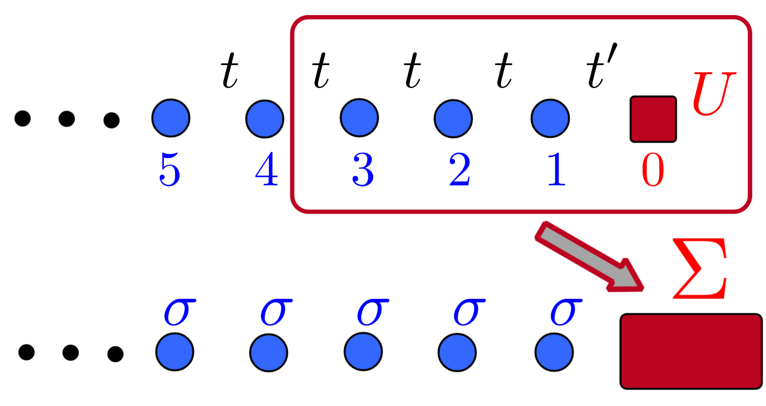
Figure 1: Upper part. Representation of a single-band Anderson impurity model with first nearest neighbor hopping. Each site (bath and impurity) has the elementary spin degree of freedom $\sigma=\pm 1/2$. Lower part. Equivalent representation of the same model where the impurity and a portion of the bath are formally considered as a larger impurity with effective elementary degree of freedom $\Sigma$.

The Method.— In order to illustrate our method, it is convenient to observe that the subsystem of $\hat{H}_{\text{imp}}$ consisting of the impurity and the first nearest $N$ bath sites can be equivalently regarded as a larger impurity $\hat{S}_{N}[\{a^{\dagger}_{\Sigma},a^{\phantom{\dagger}}_{\Sigma}\}]$, where the label $\Sigma=1,..,2(N+1)$ runs over the sites $0,..,N$ and the corresponding spins $\sigma=\pm\frac{1}{2}$, see Fig. 1. Within this definition, $\hat{H}_{\text{imp}}$ can be schematically represented as follows:

$$\hat{H}_{\text{imp}}=\hat{S}_{N}[\{a^{\dagger}_{\Sigma},a^{\phantom{\dagger}}_{\Sigma}\}]+\sum_{bb^{\prime}}[B_{N}]_{bb^{\prime}}\,b^{\dagger}_{b}b^{\phantom{\dagger}}_{b^{\prime}}$$

$$\quad+\sum_{b\Sigma}\left([V_{N}^{\dagger}]_{b\Sigma}\,b^{\dagger}_{b}a^{\phantom{\dagger}}_{\Sigma}+[V_{N}^{\phantom{\dagger}}]_{\Sigma b}\,a^{\dagger}_{\Sigma}b^{\phantom{\dagger}}_{b}\right)\,,$$ (6)

where the hybridization function $\Delta_{N}$ of $\hat{S}_{N}$

$$\Delta_{N}(z)\equiv V^{\phantom{\dagger}}_{N}\,\frac{1}{z-B_{N}}\,V_{N}^{\dagger}$$ (7)

is a well defined $M\times M$ matrix, where $M\equiv 2(N+1)$.

Our approach consists in optimizing variationally a Gutzwiller wavefunction represented as follows:

$$|\Psi_{N}\rangle\equiv\hat{\mathcal{P}}_{N}\,|\Psi_{0}\rangle\,,$$ (8)

where $|\Psi_{0}\rangle$ is a generic Slater determinant, and $\hat{\mathcal{P}}_{N}$, which is called “Gutzwiller projector”, is the most general operator acting within the subsystem $\hat{S}_{N}$. As in the ordinary Gutzwiller approximation scheme, in order to simplify the task of calculating the expectation value of the Hamiltonian [Eq. (6)], the variational freedom is further restricted by assuming the following conditions:

$$\langle\Psi_{0}|\,\hat{\mathcal{P}}_{N}^{\dagger}\hat{\mathcal{P}}^{\phantom{\dagger}}_{N}\,|\Psi_{0}\rangle\!\! = \!\!\langle\Psi_{0}|\Psi_{0}\rangle=1$$ (9)

$$\langle\Psi_{0}|\,\hat{\mathcal{P}}_{N}^{\dagger}\hat{\mathcal{P}}^{\phantom{\dagger}}_{N}\,a^{\dagger}_{\Sigma}a^{\phantom{\dagger}}_{\Sigma^{\prime}}\,|\Psi_{0}\rangle\!\! = \!\!\langle\Psi_{0}|\,a^{\dagger}_{\Sigma}a^{\phantom{\dagger}}_{\Sigma^{\prime}}\,|\Psi_{0}\rangle\;\,\forall\;\Sigma,\Sigma^{\prime}\,,$$ (10)

which are called “Gutzwiller constraints”. We point out that, while for bulk systems the Gutzwiller variational ansatz is supplemented by the so called “Gutzwiller approximation” Gutzwiller (1965), for impurity models the method is purely variational, and no further approximation is needed Lanatà et al. (2015); Lanatà (2010); Lanatà and Strand (2012).

For $N=0$ the procedure described above reduces to applying the Gutzwiller projector only onto the correlated impurity — which is the standard Gutzwiller approach for the AIM used, e.g., in Refs. Lanatà (2010); Lanatà and Strand (2012). In this work, instead, the region of action of the Gutzwiller projector is extended systematically by increasing $N$ until the desired level of accuracy is obtained.

The most evident difficulty to be overcome is that the number of complex independent parameters defining $\hat{\mathcal{P}}_{N}$ scales as $2^{2M}$. In fact, this makes the task of minimizing the total energy with respect to the wavefunction [Eq. (8)] nontrivial already for small $N$. However, fortunately, this technical problem can be efficiently solved even for relatively large $N$ thanks to the method of Refs. Lanatà et al. (2008, 2015, 2015), which is summarized in the supplemental material for completeness. A remarkable aspect of this numerical scheme is that it enables us to map the above nonlinear constrained minimization into the much simpler task of calculating iteratively the ground state $|\Phi\rangle$ of a finite AIM represented as follows:

$$\hat{H}^{\text{emb}}[\mathcal{D},\lambda^{c}]\equiv\hat{S}_{N}[\{{a}^{\dagger}_{\Sigma},{a}^{\phantom{\dagger}}_{\Sigma}\}]$$

$$\quad+\sum_{s\Sigma=1}^{M}\left(\mathcal{D}_{s\Sigma}\,{a}^{\dagger}_{\Sigma}{f}^{\phantom{\dagger}}_{s}+\text{H.c.}\right)+\sum_{ss^{\prime}=1}^{M}\lambda^{c}_{ss^{\prime}}{f}^{\phantom{\dagger}}_{s^{\prime}}{f}^{\dagger}_{s}$$ (11)

at half-filling, i.e., within the subspace such that:

$$\left[\sum_{\Sigma=1}^{M}{a}^{\dagger}_{\Sigma}{a}^{\phantom{\dagger}}_{\Sigma}+\sum_{s=1}^{M}{f}^{\dagger}_{s}{f}^{\phantom{\dagger}}_{s}\right]|\Phi\rangle=M\,|\Phi\rangle\,.$$ (12)

The complex coefficients $\mathcal{D}_{s\Sigma}$ and $\lambda^{c}_{ss^{\prime}}$ have to be determined numerically following the procedure summarized in the supplemental material. The number of AIM represented as in Eq. (11) to be solved in order to converge scales as $o(M^{2})$, and they can be solved independently (in parallel) if necessary.

As shown in the supplemental material, the ground state $|\Phi\rangle$ of $\hat{H}^{\text{emb}}$ for the converged parameters $\mathcal{D}$ and $\lambda^{c}$ encodes the expectation value with respect to the corresponding Gutzwiller wavefunction Eq. (8) of any observable $\hat{A}$ in $\hat{S}_{N}$, i.e.:

$$\langle\Psi_{N}|\,\hat{A}[\{{a}^{\dagger}_{\Sigma},{a}^{\phantom{\dagger}}_{\Sigma}\}]\,|\Psi_{N}\rangle=\langle\Phi|\,\hat{A}[\{{a}^{\dagger}_{\Sigma},{a}^{\phantom{\dagger}}_{\Sigma}\}]\,|\Phi\rangle\,.$$ (13)

For this reason, as in Ref. Lanatà et al. (2015), here we call $\hat{H}^{\text{emb}}$ “embedding Hamiltonian”. Concerning the fact that in Eq. (11) the subsystem $\hat{S}_{N}$ is coupled with a bath of equal dimension, it is interesting to observe that, at least in principle, a Hamiltonian whose bath has the same dimension of the impurity is sufficient to represent exactly the impurity ground-state properties of any system (no matter how big it is). This fact can be readily demonstrated making use of the Schmidt decomposition Peschel (2012); Knizia and Chan (2012).

Let us now discuss how the computational effort to calculate the ground state of $\hat{H}^{\text{emb}}$ scales with $M$. In order to answer this question it is important to note that $\hat{H}^{\text{emb}}$ is quadratic for all degrees of freedom made exception for those corresponding to $\{c^{\dagger}_{0,\sigma},c^{\phantom{\dagger}}_{0,\sigma}\}$ within the original representation of the AIM, see Eq. (1). Thanks to this observation, Eq. (11) can be always transformed into a finite one-dimensional chain by tridiagonalization Hewson (1997). This enables us to calculate $|\Phi\rangle$ using efficient techniques such as DMRG Saberi et al. (2008); Weichselbaum et al. (2009), whose computational cost grows only polynomially with $M$ rather than exponentially. Note that in order to perform the specific calculations that we are going to discuss in this work it has not been actually necessary to resort to this stratagem. However, this might be needed in order to study impurity models more complicated than Eq. (1).

We point out that the possibility to incorporate DMRG within our algorithm constitutes a further connection between GRG and the VRG methods mentioned in the introduction (see also Refs. Chou et al. (2012a, b)), as it reflects the fact that our approach can enforce the low-entanglement property of the ground state within the framework of the Gutzwiller wavefunction, and exploit simultaneously both of these ideas .

From the considerations above we deduce that the computational complexity of the GRG algorithm scales polynomially with $N$, i.e., with the size of the region of action of the Gutzwiller projector. Our remaining task is to understand how big $N$ has to be in order to describe accurately the ground state of the AIM.

Benchmark calculations.— In order to assess the quality of the GRG variational ansatz, here we perform benchmark calculations of the single-band AIM at half-filling, see Eq. (1).

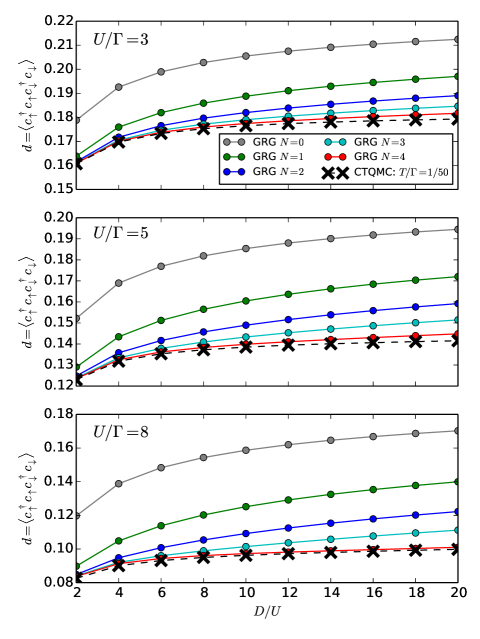
Figure 2: (Color online) Convergence of the GRG expectation value of the double occupancy $d$ with respect to the number of conduction-bath sites $N$ included within the projected region. The result is shown for different $U/\Gamma$ and $D/U$ in comparison with CTQMC (black crosses).

In Fig. 2 is shown the behavior of the impurity double occupancy $d$ as a function of $D/U$ for different values of $U/\Gamma$. The GRG results obtained with different values of $N$ are shown in comparison with continuous time quantum Monte Carlo (CTQMC) Rubtsov et al. (2005); Werner et al. (2006) as implemented in TRIQS Parcollet et al. (2015), which were obtained at temperature $T/\Gamma=0.02$. From these calculations it emerges that the $N=4$ GRG wavefunction is already sufficient to reproduce very accurately the CTQMC double occupancy for all of the interaction parameters considered. However, we observe that the convergence of $d$ with respect to $N$ becomes increasingly slower for larger $D/U$, while it is not very sensitive to $U/\Gamma$. It is interesting to compare this trend with the behavior of the dimension $\xi_{K}$ of the Kondo cloud. From the Bethe ansatz solution of the single band AIM we know that, in the large-$D$ limit, $\xi_{K}$ is given by Hewson (1997):

$$\xi_{K}\equiv v_{F}/T_{K}\sim\frac{D}{U}\sqrt{\frac{2U}{\Gamma}}e^{\frac{\pi}{8}\frac{U}{\Gamma}+\frac{\pi}{2}\frac{\Gamma}{U}}$$ (14)

(in units of the lattice spacing). As we see from Eq. (14), $\xi_{K}$ diverges exponentially with $U/\Gamma$. Furthermore, we note that $\xi_{K}$ is much bigger than the value of $N$ necessary to achieve convergence within the GRG. In fact, for instance, substituting the values $D/U=10$ and $U/\Gamma=5$ in Eq. (14) we find that $\xi_{K}\sim 275\gg 5$. Thus, we deduce that these two length scales are not directly related, as one might naively expect.

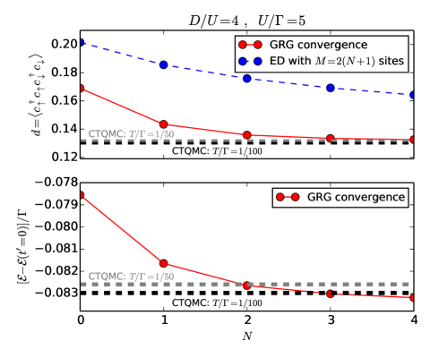
Figure 3: (Color online) Upper panel: Convergence as a function of $N$ of the GRG double occupancy $d$ for $D/U=4$ and $U/\Gamma=3$ in comparison with exact diagonalization for the truncated system composed by $2(N+1)$ sites. Lower panel: Corresponding convergence of the total energy $\mathcal{E}$. The results calculated with CTQMC are indicated by the dotted horizontal lines.

In Fig. 3 is shown the behavior of the impurity double occupancy and of the total energy calculated with GRG as a function of the convergence parameter $N$. Note that the zero of the total energy is conventionally assumed to be the ground state energy of Eq. (1) with $t^{\prime}=0$. These data are shown in comparison with CTQMC and with the exact diagonalization results obtained by taking into account only the first $2(N+1)$ sites of Eq. (1) (and discarding the others).

We observe that both the GRG energy and double occupancy converge very rapidly to their respective exact values. From this observation we argue that the above mentioned GRG convergence concerns the entire ground state of the AIM, and not only the expectation value of the impurity degrees of freedom.

From the comparison between GRG and exact diagonalization it emerges that the dimension of the auxiliary AIM [Eq. (11)] to be solved in order to calculate the GRG solution of any order $N$ is much smaller than the dimension of the truncated AIM that would enable us to solve the problem with comparable precision directly with DMRG Weichselbaum et al. (2009). Thus, as discussed before, using DMRG to solve iteratively Eq. (11) within the GRG algorithm seems to be a more convenient option.

Conclusions.— In summary, we have developed a variational method called GRG, that takes advantage simultaneously of two among the most powerful ideas in condensed matter theory: (1) the Gutzwiller wavefunction, that enables us to incorporate the most general single-particle wavefunction (Slater determinant) within the variational space, thus reducing the many-body problem to correcting variationally the corresponding electron configurations with the “Gutzwiller projector”; (2) the VRG methods, that enable us to exploit the fact that the ground state of the AIM has low-entanglement (once the problem is formulated in one dimension). Using the GRG, we have shown that the ground state of the AIM has a very simple structure, which can be represented very accurately in terms of a surprisingly small number of variational parameters. These insights resulted in an efficient algorithm that might enable us to study complex systems beyond the reach of any other method presently available. Another remarkable property of our approach is that it enables us to describe the ground state of the AIM directly in the thermodynamical limit and at all length scales, while this is technically very difficult with the other VRG methods, which require to truncate part of the chain. Our work paves the way to several generalizations. In particular, it will be very interesting to generalize it to finite temperatures Lanatà et al. (2015) and to nonequilibrium transport in nanostructures, see Refs. Lanatà (2010); Lanatà and Strand (2012). In fact, the physics of the AIM out of equilibrium is not still well understood, and different methods seem to produce different results even for simple systems such as the single band AIM Dirks et al. (2013).