Morfometryka – A New Way of Establishing Morphological Classification of Galaxies

Abstract

We present an extended morphometric system to automatically classify galaxies from astronomical images. The new system includes the original and modified versions of the CASGM coefficients (Concentration $C_{1}$, Asymmetry $A_{3}$, and Smoothness $S_{3}$), and the new parameters entropy, $H$, and spirality $\sigma_{\psi}$. The new parameters $A_{3}$, $S_{3}$ and $H$ are better to discriminate galaxy classes than $A_{1}$, $S_{1}$ and $G$, respectively. The new parameter $\sigma_{\psi}$ captures the amount of non-radial pattern on the image and is almost linearly dependent on T-type. Using a sample of spiral and elliptical galaxies from the Galaxy Zoo project as a training set, we employed the Linear Discriminant Analysis (LDA) technique to classify Baillard et al. (2011, 4478 galaxies), Nair & Abraham (2010, 14123 galaxies) and SDSS Legacy (779,235 galaxies) samples. The cross-validation test shows that we can achieve an accuracy of more than 90% with our classification scheme. Therefore, we are able to define a plane in the morphometric parameter space that separates the elliptical and spiral classes with a mismatch between classes smaller than 10%. We use the distance to this plane as a morphometric index (M_i) and we show that it follows the human based T-type index very closely. We calculate morphometric index M_i for $\sim$780k galaxies from SDSS Legacy Survey - DR7. We discuss how M_i correlates with stellar population parameters obtained using the spectra available from SDSS-DR7.

1. Introduction

The study of the formation and evolution of galaxies in general requires their systematic observations over a large redshift domain. Datasets for local (today^′s systems) and distant galaxies (their actual progenitors) must be consistently gathered to avoid biases, a procedure that requires a knowledge of the very evolution we are seeking to understand. From an astrophysical perspective, mechanisms regulating star formation, e.g. ram-pressure (Gunn & Gott, 1972), harassment (Moore et al., 1996), starvation (Larson et al., 1980), depend on the distance from the center of the potential well of a cluster; their effects on the stellar population of a galaxy depend on how efficiently the local environment is capable of removing the interstellar gas and affect the star formation history. Thus, morphology, in a general sense, is just a snapshot reflecting all these processes imprinted in the galaxy image at a given time.

Traditionally, galaxy morphology has been addressed visually: an expert examines the images of galaxies and identifies features (or absence of them, in the case of early-type galaxies) which distinguish the object as belonging to a specific class, as done in Hubble (1926); de Vaucouleurs (1959); Sandage (1975); van den Bergh (1976); Lintott et al. (2008, 2011), among many others. This classification paradigm is strongly subjective, prone to errors and cannot be applied to the number of galaxies present in modern surveys For instance, Fasano et al. (2012) compare their classification with that of de Vaucouleurs et al. (1991, RC3 catalog) (see their Figure 2). As it is clearly seen there is an uncertainty of approximately 1 in T-type within Fasano et al. (2012) authors and about 2.5 between RC3 and Fasano et al. (2012). Comparison between EFIGI and NA2010, for 1438 galaxies in common (Baillard et al., 2011, Figure 32), exhibits a similar sort of inconsistency, with an uncertainty between 2 and 3 in T-type. This tell us that, for example, visual classification does not agree when distinguishing an S0 from an Sa or an E from an S0. Thus, it is imperative to quantify the morphology of a galaxy as a measurable quantity – morphometry – that can be coded in an algorithm. However, in spite of its uncertainties, visual classification is still important, because automated techniques would have difficulty doing classifications like ${\rm(R_{1}R_{2}^{\prime})SAB(r,nr)0/a}$ which is much more valuable than just knowing whether a galaxy is S, S0, or E. Also, regarding RC3, it should be noted that its classifications were made based on photographic plates or sky survey charts. Modern digital images allow greater consistency between multiple classifiers and have the potential to greatly improve on RC3.

Two approaches for galaxy morphometry have been widely explored recently: parametric – those which model the light distribution as a bulge plus disk plus other less important components representing a few percent of the total light (e.g. Peng et al., 2002; Simard et al., 2002); non-parametric – those which use the measured properties of the light distribution, like concentration, asymmetry (e.g. Abraham et al., 1996). Each approach has its virtues and vices, as discussed for example in Andrae et al. (2011).

One relatively successful non-parametric system is the concentration, asymmetry, smoothness, Gini and M20 (CASGM) system, presented in Abraham et al. (1994, 1996), Conselice et al. (2000) and Lotz et al. (2004). This basic set has been enlarged with other quantities such as the Sérsic model parameters (Sersic, 1967), and the Petrosian radius (Petrosian, 1976), among others. These quantities may not work properly in the high redshift regime and this has been studied in recent papers (e.g. Freeman et al., 2013). These authors use Multi-mode, Intensity and Deviation statistics, MID, to detect disturbances in the galaxy light distribution and show that it is very effective at z $\sim$2.

The previously mentioned way of establishing galaxy morphology answers two immediate needs. First, it is possible to reproduce human classification by positioning the galaxies in the space of these parameters. In such a supervised classification, a set of visually classified galaxies are used to train a discriminant function that will assign to each new galaxy a probability of belonging to each class. The second reason for establishing a galaxy morphometry system is that we can seek structures, in the quantitative morphology parameter space, that may yield clues for the physical reasons for their formation and evolution that are not visible in the currently human-based mode. Further, a system such as the Hubble tuning fork classification does not account for all the details that we can currently measure in galaxy images, and it does not hold as we go deep even at a moderate redshift $z=0.25$. To evaluate this, a new quantitative classification procedure is needed, both to handle the large amount of data becoming available with the new surveys, and also to help us find the physical processes driving galaxy evolution.

The paper is organized as follows: in Section 2 we discuss similar works; in Section 3 we describe the datasets used; in Section 4 we define new nonparametric methods to quantify galaxy morphology; in Section 5 we present the Morfometryka algorithm. We apply the Morfometryka code to galaxy samples described in Section 6, where we also test the robustness of the measured parameters and explore the ability of them to classify galaxy morphologies. In Section 7 we propose a new Morphometric Index M_i. In Section 8 we compare M_i with other physical parameters and summary is presented in Section 9.

2. Related Work

There have been several attempts to classify galaxies automatically, beginning with Abraham et al. (1994, 1996), among others. Here we briefly mention recent works based on machine learning and on morphometric parameters. The list is not meant to be exhaustive but rather to present different approaches followed in the last few years.

Huertas-Company et al. (2011) used a system based on colors, shapes and concentration to train a support vector machine to classify $\sim$700k galaxies from the SDSS DR7 spectroscopic sample. For each galaxy, they estimate the probabilities of being E, S0, Sab or Scd. It is not a pure morphometric classification, since it includes colors.

Scarlata et al. (2007) analyses 56,000 COSMOS galaxies with the ZEST algorithm, using five nonparametric diagnostics ($A$, $C_{1}$, $G$, $M_{20}$, $q$) and Sérsic index $n$. They perform Principal Component Analysis (PCA) and classify galaxies with 3 principal components. They find contamination between galaxy classes in parameters space (see their Fig.10), although they do not state clearly the success rate of the classification.

Andrae et al. (2011) present a detailed analysis of several critical issues when dealing with galaxy morphology and classification. Several morphological features are intertwined and cannot be estimated independently. They show the dependence between $C$ and $n$, which is also presented here in a different form in Appendix C. The authors claim that parameter based approaches are better for classification, and state that a system such as CASGM has serious problems. However, they do not show it in practice.

Dieleman et al. (2015) present a Neural Network machine to reproduce Galaxy Zoo classification. They work directly in pixel space, using a rotation invariant convolution that minimizes sensitiveness to changes in scale, rotation, translation and sampling of the image. The algorithm obtains an accuracy of 99% relative to the Galaxy Zoo human classification; however, since the human classification is also error prone, as discussed in Section 1, their algorithm reproduces also the errors in the human classification.

Freeman et al. (2013) introduced MID (multimode, intensity and deviation) statistics designed to detect disturbed morphologies, and then classify 1639 galaxies observed with HST WFPC3 with a random forest. It is one of the few works that state the detailed classifier performance, in terms of the confusion matrix coefficients.

3. Data and Sample Selection

	EFIGI	NA	LEGACY	LEGACY$-zr$
Total	4 458	14 034	804 974	337 097
mfmtk	4 214	12 729	779 235	327 937
mfmtk+Zoo	1 856	8 792	245 206	125 417

Table 1Number of objects in the databases used in this work. MFMTK are objects for which Morfometryka made measurements; Zoo means objects classified as E or S by Galaxy Zoo.

We use several databases derived from SDSS DR7 (Abazajian et al., 2009), for which we analyze $r$ band images. They are: the Baillard et al. (2011) database (hereafter EFIGI); the Nair & Abraham (2010) database (hereafter NA); and the SDSS DR7 complete Legacy database and a volume limited subsample, hereafter referred as LEGACY and LEGACY–$zr$, respectively. We also use the Galaxy Zoo collaborative project visual classification (Lintott et al., 2008, 2011). The number of galaxies in the original databases, those succesfully processed by Morfometryka and those that have a Galaxy Zoo classification are listed in Table 1.

The databases are used with different purposes, namely, training, validation and classification. In training phase, the galaxies in the databases that have Galaxy Zoo classification are used to train a classifier machine (Section 6.2). For validation, we use a cross validation scheme to attest how well our classifier performed compared to Galaxy Zoo human classification. In the classification stage, we use the trained classifier to linearly separate LEGACY galaxies in two classes (elliptical–E or spiral–S) in the morphometric parameters space (Section 6.2). The galaxy distance to the separating hyperplane is then proposed as a morphometric index $M_{\rm i}$ (Section 7). The databases EFIGI and NA, for which we have T-type values, are further used to support out argument that $M_{\rm i}$, based on the classifier discriminant function, can reflect the galaxy morphological type.

The classification scheme from the Galaxy Zoo project (Lintott et al., 2008, 2011) was used to train our supervised morphometric classifier. The Galaxy Zoo project provides simple morphological classifications of nearly 900,000 galaxies drawn from the SDSS-DR6.

Below we discuss each sample in detail.

3.1. The EFIGI sample

The EFIGI catalog was specifically designed to sample all Hubble morphological types. It provides detailed morphological information of galaxies selected from standard surveys and catalogues (Principal Galaxy Catalogue, Sloan Digital Sky Survey, Value-Added Galaxy Catalogue, HyperLeda, and the NASA Extragalactic Database). The sample is essentially limited in apparent diameter, and offers a detailed view of the whole Hubble sequence. The final EFIGI sample comprises 4458 galaxies for which there is imaging in all the $ugriz$ bands in the SDSS-DR4 database. For these galaxies, the EFIGI reference dataset provides visually estimated morphological information as well as re-sampled SDSS imaging data. The photometric catalog is more than   80% complete for galaxies with $10<m_{{\rm petro},g}<14$, where $m_{{\rm petro},g}$ is the Petrosian magnitude in the $g$ band.

3.2. The NA sample

Nair & Abraham (2010) provide detailed visual classifications for 14034 galaxies selected from the SDSS spectroscopic main sample described in Strauss et al. (2002). They used the SDSS-DR4 photometry catalogs to select all spectroscopically targeted galaxies in the redshift range $0.01<z<0.1$ down to an apparent extinction-corrected magnitude limit of $g<16$ mag. Objects mistakenly classified as galaxies have been removed, leading to the final sample of 14,034 galaxies. Their final catalog provides T-Types, the existence of bars, rings, lenses, tails, warps, dust lanes, arm flocculence, and multiplicity for all galaxies.

3.3. The SDSS LEGACY and LEGACY–$zr$ samples

Our target sample of galaxies was retrieved from SDSS-DR7 (Abazajian et al., 2009) by selecting all objects spectroscopically classified as galaxies (see Appendix A.2 for full query). SDSS Frames and psFields were obtained and stamps and PSF (point spread function) generated from them (see Appendix A for details). Our final catalog comprises 804,974 objects.

The subsample LEGACY–$zr$ is volume limited at redshift $z<0.1$ and $m_{{\rm petro},r}<17.78$, where $m_{{\rm petro},r}$ is the extinction corrected Petrosian magnitude in the $r$ band. This magnitute limit roughly corresponds to the magnitude at which the SDSS spectroscopy is complete (Strauss et al., 2002). The redshift limit of $z<0.1$ provides a complete sample for $M_{\rm petro,r}<-20.5$, where $M_{\rm petro,r}$ is the SDSS Petrosian absolute magnitude in the $r$ band.

For 570,685 galaxies, those for which zWarning=0 in the SDSS database, we derived ages, metallicities, stellar masses and velocity dispersions using the spectral fitting code starlight (Cid Fernandes et al., 2005). Before running the code, the observed spectra are corrected for foreground extinction and de-redshifted, and the single stellar population (SSP) models are degraded to match the wavelength-dependent resolution of the SDSS spectra, as described in La Barbera et al. (2010). We adopted the Cardelli et al. (1989) extinction law, assuming $R_{\rm V}=3.1$.

We used SSP models based on the Medium resolution INT Library of Empirical Spectra (MILES, Sánchez-Blázquez et al., 2006), using the code presented in Vazdekis et al. (2010), using version 9.1 (Falcón-Barroso et al., 2011). They have a spectral resolution of $\sim 2.5$ Å, almost constant with wavelength. We selected models computed with Kroupa (2001) Universal IMF with slope $=1.30$, and isochrones by Girardi et al. (2000). The basis grids cover ages in the range of $0.07-14.2$ Gyr, with constant $\log({\rm Age})$ steps of 0.2. We selected SSPs with metallicities [M/H] =$\{-1.71,-0.71,-0.38,0.00,+0.20\}$.

4. Quantitative galaxy morphology

The basic morphometric measurements of the CASGM system are fully described by Abraham et al. (1994, 1996), Bershady et al. (2000), Conselice et al. (2000) and Lotz et al. (2004), among others. Relevant modifications of these parameters and the new parameters introduced in this work are discussed in this section.

We define the region with the same axis ratio and position angle as the galaxy (see Section A.2) and with major axis equal $N_{\!R_{p}}R_{p}$, where $R_{p}$ is the Petrosian Radius and $N_{\!R_{p}}=2$, as the Petrosian region. Most measurements are made with pixels in this regions, except if otherwise stated. A central region of the size of the PSF FWHM is masked before calculating $A$, $S$ and $\sigma_{\psi}$.

4.1. Concentration $C_{1}$ and $C_{2}$

The concentration index $C$ is the ratio of the circular radii containing two fractions of the total flux of the galaxy (Kent, 1985), where these percentages are chosen to maximize the distinction between systems and minimize seeing effects. The concentration depends on the determination of the radius that contain some fraction of some measure of the total luminosity of the galaxy. In this work, we have adopted the Petrosian luminosity as the total luminosity $L_{T}$, which is the maximum value of $L(R)$ inside the Petrosian region. The measured $L(R)$ is spline interpolated and then the point where it attains some fraction $f$ of $L_{T}$ is found by evaluating the spline at the point. In this way we obtain $R_{20}$, $R_{50}$, $R_{80}$ and $R_{90}$ and finally

$$C_{1}=\log_{10}{\left(\frac{R_{80}}{R_{20}}\right)}\qquad\text{and}\qquad C_{2}=\log_{10}{\left(\frac{R_{90}}{R_{50}}\right)}.$$

Note that we dropped the factor 5 usually in the definition of $C$, so that all morphometric measurements used will fall approximately in the range $[0,1]$, and thus statistic standardization would have little effect and may be optional. The concentration $C_{1}$ is more sensitive to seeing effect that is more pronounced in the central regions and thus on $R_{20}$; $C_{2}$ is more sensitive to noise that is more important in the outer regions and thus on the measure of $R_{90}$.

4.2. Asymmetry $A_{1}$, $A_{2}$, $A_{3}$

The asymmetry coefficient $A$ is determined comparing a source image with its rotated counterpart. We measure the asymmetry $A_{1}$, as defined by Abraham et al. (1996), with the exception that we do not subtract the background asymmetry, for we find that this procedure makes the asymmetry estimation unstable and sensitive to the selected sky (an hence to the stamp) size. Instead, we consider only the galaxy portion inside the Petrosian region. Even so, $A_{1}$ depends heavily on the noise and on the image sampling. To address this problems we used two new asymmetry measurements defined as

$$A_{2}=1-r(I,I_{\pi})$$ (1)

and

$$A_{3}=1-s(I,I_{\pi})$$ (2)

where $r()$ and $s()$ are the Pearson and Spearman correlation coefficients (Press et al., 2002), respectively, $I$ is the image and $I_{\pi}$ its $\pi$-rotated version. The rationale behind this formulation is that those pixels made up mostly of noise will not contribute to $A_{2}$ and $A_{3}$ since the correlation between them will tend to zero. Further, correlation coefficients are more immune to convolution and thus less affected by seeing effects. The Pearson coefficient tends to accumulate close to unity and so $A_{2}$ has proven not so useful as $A_{1}$ and $A_{3}$. The center of rotation is chosen to minimize the asymmetry measurements.

4.3. Gini coefficient

The Gini coefficient $G$ measures the flux distribution among the pixels of a galaxy image. The Gini coefficient for the image pixels in the Petrosian region is calculated exactly as shown in Lotz et al. (2004), i.e., for $n$ pixels with values $I_{i}$ in increasing order we have

$$G=\frac{1}{n(n-1)\,\bar{I}}\ \sum\limits_{i}^{n}(2i-n-1)\,I_{i},$$

where $\bar{I}$ is the average value.

4.4. Smoothness

The smoothness coefficient $S$ (a.k.a clumpiness) in general measures the small scale structures in the galaxy image. Here we consider three different measures of smoothness. $S_{1}$ is calculated as shown in Lotz et al. (2004), except that the filter used is a Hamming window (Hamming, 1998) with size $\lceil R_{p}/4\rceil$. Following the same reasoning as for asymmetry, we define the modified smoothness $S_{2}$ and $S_{3}$ as

$$S_{2}=1-r(I,I^{F})$$ (3)

and

$$S_{3}=1-s(I,I^{F})$$ (4)

where $I^{F}$ is the filtered image. As with asymmetry, $S_{3}$ has proven to be more useful than $S_{2}$.

4.5. Entropy

The entropy of information $H$ (Shannon entropy, e.g. Bishop (2007)) is used here to quantify the distribution of pixel values in the image. For a random variable $I$, the entropy $H(I)$ is the expected value of the information $\log[p(I)]$

$$H(I)=-\sum_{k}^{K}\;p(I_{k})\;\log[p(I_{k})],$$ (5)

where $p(I_{k})$ is the probability of occurrence of the value $I_{k}$, $k$ refers to a specific value and $K$ is the number of bins considered. For discrete variables, $H$ reaches the maximum value for a uniform distribution, when $p(I_{k})=1/K$ for all $k$ and hence $H_{\rm max}=\log K$. The minimum entropy is that of a delta function, for which $H=0$. We then have the normalized entropy

$$\widetilde{H}(I)=\frac{H(I)}{H_{\rm max}}\qquad 0\leqslant\widetilde{H}(I)\leqslant 1.$$ (6)

Smooth galaxies will have low $H$ while clumpy will have high $H$.

4.6. Spirality $\sigma_{\psi}$

None of the CASGM parameters take into account the spiral arms, rings and bars in galaxies, albeit they are a major and important emphasis of human based classification. We devise a parameter to take it into account. As done in Shamir (2011), we first transform the standardized galaxy image to polar coordinates $(r,\theta)$. In $(r,\theta)$ space a bulge appears as a band in the lower region of the diagram, a bar as two vertical lines and spiral arms as inclined bands. See Figure 1. We then calculate the gradient magnitude $|\nabla I|$ and direction $\vec{\psi}$ fields of the polar image. Most points in this direction field $\vec{\psi}$ for an elliptical galaxy will point to the bottom, whilst for a spiral galaxy there will be many orientations corresponding to arms, rings and bars. The standard deviation $\sigma_{\psi}$ for the field direction values will be smaller for an elliptical compared to that of a spiral, and hence can be used to estimate the amount of characteristic structures. To avoid regions of noise, we make the measurements in regions where the gradient magnitude is greater than the median of the magnitude field.

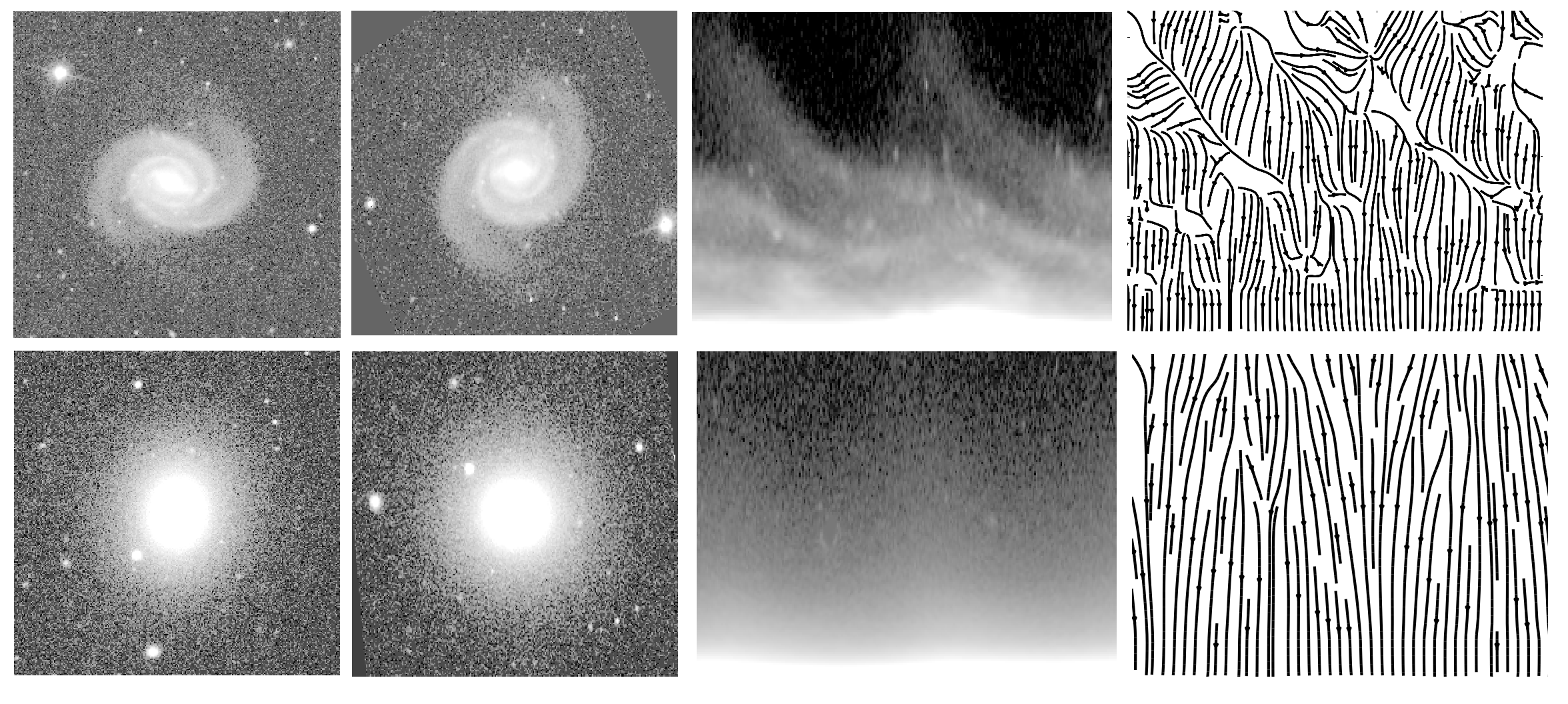
Figure 1.— Illustration about how spirality is measured. EFIGI spiral SB PGC 2182 above and lenticular PGC 2076 below. From left to right: original image, standardized image ($q=1$, $PA=0^{\circ}{}$), image in polar coordinates, gradient field of polar image.

Figure 2 shows a density plot of $\sigma_{\psi}$ versus T-type for the EFIGI database (a subsample of galaxies were selected such that there are 45 objects in each T-type), where a clear linear relationship is seen. So, $\sigma_{\psi}$ is a good diagnostic for T-type, provided there is enough spatial resolution to distinguish spiral arms, rings and bars. This is the case for EFIGI database, marginally for NA and not for LEGACY in general, as inferred from the discussion in Section 6.1 and Figure 4.

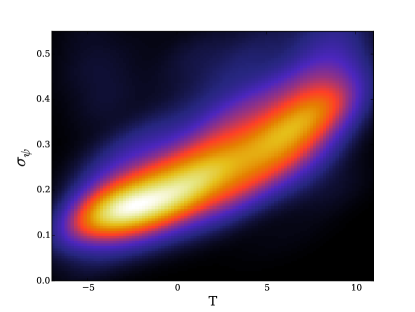
Figure 2.— Density plot for $\sigma_{\psi}$ versus T-type for the EFIGI sample. For this plot, a subsample of galaxies were selected so that there is 45 galaxies in each T-type.

5. The Morfometryka algorithm

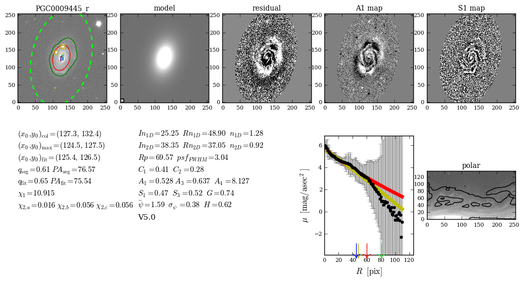
Figure 3.— Example Morfometryka graphical output for EFIGI $r$-band image of PGC 9445 (ObjID-DR7 587 731 513 150 734 392). Top, from left to right: PGC0009445_r: original image (dark green line is primary segmentation, red line is 2D Sérsic fit $R_{n}$, dotted light green line is Petrosian region of 2 $R_{p}$, color caracters mark different centers); model: 2D Sérsic model image (insert showing the PSF at bottom left); residual: image minus 2D Sérsic model residual; A1 map: asymmetry map used to compute $A_{1}$; S1 map: Smoothness map used to $S_{1}$. Bottom:, left to right: various measurements (see text for details); brightness profile (arbitrary units): black dots are measurements, red line 1D and yellow line 2D Sérsic fits. polar: map used to compute image gradient and $\sigma_{\psi}$. Its morphometric index is $M_{\rm i}=0.16$

We developed a standalone application to automatically perform all the structural and morphometric measurements over a galaxy image, called Morfometryka (mfmtk). mfmtk reads the input stamp image and related PSF for a given galaxy and performs various measurements explained in detail in Appendix A. mfmtk is currently implemented in an object-oriented fashion in Python 2.7, with the aid of scientific libraries SciPy and Numpy (Oliphant (2007)), Matplotlib (Hunter (2007)) and PyFits.

The Morfometryka basic output is: sky background value and standard deviation; image centers $(x_{0},y_{0})_{\rm CoL}$, $(x_{0},y_{0})_{\rm peak}$; Sérsic parameters for 1D surface brightness profile fitting ($I_{n1D};R_{n1D};n_{1D}$) and for 2D image fitting ($I_{n2D},R_{n2D},n_{2D},q_{2D},PA_{2D},(x_{0},y_{0})_{2D}$), Petrosian Radius $R_{p}$; radii $R_{20},R_{50},R_{80},R_{90}$ and concentrations $C_{1}$ and $C_{2}$; asymmetries $A_{1},A_{2},A_{3}$ and fitted center for $A_{1}$ and $A_{3}$; smoothness $S_{1}$ and $S_{3}$; Gini coefficient $G$; second moment $M_{20}$; gradient field direction value $\psi$ and standard deviation $\sigma_{\psi}$; quality flags QF. Optionally, all maps (star masks, segmentation map, polar image and so on) are saved. Morfometryka takes about 12 seconds to process a $256\times 256$ galaxy and $45\times 45$ PSF image on a 2.5 Ghz processor. The version used in this work was 5.0.

6. Supervised Classification

Our morphological classification is based on the linear discriminant method which separates galaxies in two main classes (E and S) in morphometric parameters space. We train the classifier using the classification from the Galaxy Zoo (Lintott et al., 2008, 2011). The process was done independently for EFIGI, NA, LEGACY and LEGACY$-zr$ datasets.

Our main goal is not only to classify galaxies in a way that reproduces the human classification but also to establish a basis for a morphometric space where galaxy classes are separated allowing further studies where the human classifier cannot be used. Thus, we use a linear discriminant and also we seek for the smallest set of independent parameters that may yield a reliable classification which is physically meaningful.

6.1. Feature Selection

Given that we have so many measured quantities for each galaxy, some of them may be redundant or irrelevant and we need to select those which are more relevant to the classification algorithm. Many feature selection algorithms tends to diminish the importance of quantities that correlate with each other. A criterium that avoids that is the Maximum Information Content (MIC, Albanese et al. (2013)). MIC is based on the mutual information and the information entropy: it compares, given the parameters and the known class, which one possesses the greater mutual information with the class variable, i.e. which one will have greater impact in the classification. The normalized values for MIC are shown in Figure 4.

We may have more information on how efficiently each feature helps to separate the classes by examining the feature histogram separated by classes, as shown Appendix D, in Figure 10 (EFIGI), Fig. 11 (NA), Fig. 12 (LEGACY) and Fig. 13 (LEGACY$-zr$) . We must be aware that we are seeing marginal probability distribution functions (PDF) on each variable and this is not equivalent to analyse the multivariate PDF of all parameters together.

First, we note that the features with highest discriminant power are those related to the light concentration (Sérsic $n$, $C_{1}$ and $C_{2}$). Since they are equivalent (Appendix C), and also equivalent to the Petrosian Radii (Appendix B), we retain only $C_{1}$ and $C_{2}$ which are not parametric and more robust.

Comparing the asymmetry measures in the histograms in Appendix D, we see that $A_{3}$ is able to discriminate classes better than $A_{1}$, which is confirmed by the MIC values. Gini coefficient is very poor at separating E from S, as it is $M_{20}$. Compared to Gini, entropy $H$ works better in separating classes, and the introduced $S_{3}$ is better than the original $S_{1}$. The axis ratio $q$ is good for E but indifferent for S, so it is not used. The spirality $\sigma_{\psi}$ is also good to discriminate classes but it is crucially dependent on angular resolution - its importance decreases from EFIGI to NA, to LEGACY, in the same sense as the mean angular resolution decreases.

Finally, based on the MIC analysis, we choose this set of parameters

$$\textbf{x}=\left\{C_{1},A_{3},S_{3},H,\sigma_{\psi}\right\},$$

for they constitute a minimal set of independent parameters that yield a reliable classification. Four of the chosen parameters are new, used here for the first time. $A_{3}$ and $S_{3}$ are enhanced versions of standard parameters, $H$ is first applied in morphometric studies and $\sigma_{\psi}$ is completely new.

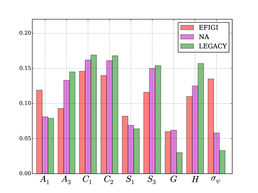
Figure 4.— Feature Relative Importance for the morphometric parameters as calculated by the Maximum Information Content criterion.

6.2. Linear Discriminant Analysis

A simple linear classifier may be represented by a discriminant function which for a given input vector x that contains $d$ morphometric measurements (Duda, 2001; Bishop, 2007) gives

$$f(\textbf{x})=\textbf{w}^{T}\textbf{x}+w_{0},$$ (7)

where w is the weight vector and $w_{0}$ is the threshold. The input vector is assigned to the class $\mathcal{C}_{1}$ if $f(\textbf{x})>0$ and to $\mathcal{C}_{2}$ otherwise. The decision boundary or surface is a hyperplane defined by $f(\textbf{x})=0$, for which w is a normal vector and $-w_{0}/||\textbf{w}||$ its normal distance to the origin. The decision function corresponds to the perpendicular distance from x to the decision surface.

When using the Bayes Decision Theory the expressions for w and $w_{0}$ are assigned as follows: an object belongs to class $\mathcal{C}_{1}$ if

$$P(\mathcal{C}_{1},\textbf{x})>P(\mathcal{C}_{2},\textbf{x})\qquad(\text{for class }\mathcal{C}_{1})$$ (8)

and to $\mathcal{C}_{2}$ otherwise. Since the evidence $p(\textbf{x})$ is the same for both classes, Bayes rule in Eq. (8) is equivalent to

$$p(\textbf{x},\mathcal{C}_{1})\,P(\mathcal{C}_{1})>p(\textbf{x},\mathcal{C}_{2})\,P(\mathcal{C}_{2})$$ (9)

where $p(\textbf{x},\mathcal{C}_{i})$ is the class conditional probability density function (CCPDF) and $P(\mathcal{C}_{i})$ the prior. We assume that the CCPDF is multivariate normal density

$$p(\textbf{x},\mathcal{C}_{i})=\frac{1}{(2\pi)^{d/2}|\boldsymbol{\Sigma}|^{1/2}}\exp\left[-\frac{1}{2}(\textbf{x}-\boldsymbol{\mu}_{i})^{T}\,\boldsymbol{\Sigma}_{i}^{-1}(\textbf{x}-\boldsymbol{\mu}_{i})\right],$$ (10)

where $\boldsymbol{\mu}_{i}$ are the mean and $\boldsymbol{\Sigma}_{i}$ the covariance matrix of x for class $\mathcal{C}_{i}$ . The decision rule Eq. (9), or equivalently its logarithm, is then

$$-\frac{1}{2}(\textbf{x}-\boldsymbol{\mu}_{1})^{T}\,\boldsymbol{\Sigma}_{1}^{-1}(\textbf{x}-\boldsymbol{\mu}_{1})+\ln P(\mathcal{C}_{1})>$$

$$-\frac{1}{2}(\textbf{x}-\boldsymbol{\mu}_{2})^{T}\,\boldsymbol{\Sigma}_{2}^{-1}(\textbf{x}-\boldsymbol{\mu}_{2})+\ln P(\mathcal{C}_{2})$$ (11)

The terms involving $\textbf{x}^{\prime}\boldsymbol{\Sigma}_{i}^{-1}\textbf{x}^{\prime}$ are general quadratic forms and if we expand them in Eq.(6.2) we have a Quadratic classifier. But instead, we consider identical covariance matrices $\boldsymbol{\Sigma}_{1}=\boldsymbol{\Sigma}_{2}=\boldsymbol{\Sigma}$ which yield a Linear classifier. Expanding the terms in Eq.(6.2), and ignoring those that are identical for both classes, we have

$$\boldsymbol{\Sigma}^{-1}(\boldsymbol{\mu}_{1}-\boldsymbol{\mu}_{2})+\frac{1}{2}\boldsymbol{\mu}_{1}^{T}\boldsymbol{\Sigma}^{-1}\boldsymbol{\mu}_{1}+\frac{1}{2}\boldsymbol{\mu}_{2}^{T}\boldsymbol{\Sigma}^{-1}\boldsymbol{\mu}_{2}+\ln\frac{P(\mathcal{C}_{1})}{P(\mathcal{C}_{2})}>0.$$ (12)

If we refer to Eqs.7 and 12, we have then

w $$=\boldsymbol{\Sigma}^{-1}(\boldsymbol{\mu}_{1}-\boldsymbol{\mu}_{2})$$ (13)

$$w_{0} =\frac{1}{2}\boldsymbol{\mu}_{1}^{T}\boldsymbol{\Sigma}^{-1}\boldsymbol{\mu}_{1}+\frac{1}{2}\boldsymbol{\mu}_{2}^{T}\boldsymbol{\Sigma}^{-1}\boldsymbol{\mu}_{2}+\ln\frac{P(\mathcal{C}_{1})}{P(\mathcal{C}_{2})},$$ (14)

which completes our linear classifier.

6.3. Classifier Performance

We may estimate the classifier performance by means of a confusion matrix or contingency table, which is a comparison of the actual class with the predicted class for each objects. The performance is evaluated calculating several scores based on true positives (TP, hits), true negatives (TN, correct rejections), false positives (FP, false alarms) and false negatives (FN, misses). See for example Hackeling (2014).

The accuracy $A$ is the fraction of hits relative to the total number of classifications

$$A=\frac{TP+TN}{TP+TN+FP+FN};$$

Precision $P$ is the fraction of positive predictions that are correct

$$P=\frac{TP}{TP+FP};$$

Sensitivity $R$ is the fraction of the truly positive instances that the classifier recognizes

$$R=\frac{TP}{TP+FN};$$

and $F_{1}$ score which is harmonic mean between sensitivity and precision

$$F_{1}=\frac{2TP}{2TP+FP+FN}.$$

We test the performance of the classifier by a 10-fold cross validation: for each database we selected those samples with known Galaxy Zoo classification and partitioned them in 10 parts; in each of 10 runs one of the parts we used as a validation sample and the other 9 parts as training sample. In each run, the scores A, P, R, F1 were calculated; their final averages are shown in Table 2. For all databases the classifier performs usually better than 90%, namely 90% of the time the automated classifier grees with the visual classification. If we consider that the performace in the human classification is also of that order, and that those classification were used to train the classifier, then this performance can be considered very good and it is the best figure that we could expect without using a classifier that would incorporate the errors in it.

	EFIGI	NA	LEGACY	LEGACY–$zr$
$A$	0.938	0.902	0.877	0.938
$P$	0.962	0.931	0.905	0.956
$R$	0.964	0.899	0.935	0.968
$F_{1}$	0.963	0.914	0.920	0.963

Table 2Mean scores for each database for a 10-fold cross validation tests.

7. Morphometric Index

As stated in Section 6.2, the discriminant function $f(\textbf{x})$ is the distance of x to the plane that separates classes, here ellipticals and spirals. Based on that, we propose to use $f(\textbf{x})$ to represent the galaxy type, that we call the morphometric index $M_{\rm{i}}$. Figure 5 shows the comparison of $M_{\rm{i}}$ with the $T$ type from EFIGI and NA samples. There is a clear linear relationship between $M_{\rm{i}}$ and $T$ type justifying the use of $M_{\rm{i}}$ as a morphometric index. In Section 8 we extend this argument by comparing $M_{\rm i}$ with other galaxy physical characteristics. By construction, $M_{\rm i}$ is negative for early-type and positive for late-type galaxies.

A linear regression between $T$ and $M_{\rm i}$ could be used to calibrate $M_{\rm i}$ as an inferred $T$-type, but since $T$ is a subjective parameter we prefer to maintain $M_{\rm i}$ in its own scale, and as a pure morphometric measure, estimated solely based on the values of x. For a binary classification, the magnitude of the direction vector w has no importance, and in fact, $\|\textbf{w}\|$ could be different depending on the details of the LDA. But since we want to use this distance as a physical measure, we prefer to normalize w and the distance to the plane $w_{0}$ in the morphometric index $M_{\rm i}$, so that

$$M_{\rm i} =\hat{\textbf{w}}^{T}\textbf{x}+\hat{w_{0}},$$ (15)

$$\text{where}\quad\hat{\textbf{w}} =\frac{\textbf{w}}{\|\textbf{w}\|}\quad\text{and}\quad\hat{w_{0}}=\frac{w_{0}}{\|\textbf{w}\|}.$$

The final values for LEGACY database are

$$\hat{\textbf{w}} =\{-0.832,0.249,0.451,0.190,-0.079\}$$ (16)

$$\hat{w}_{0} =0.018$$ (17)

As we see in Eq.(14), $w_{0}$ depends on the class priors $P(\mathcal{C}_{i})$. Usually, the relative frequency for each class $N_{i}/N$ ($N_{i}$ the number of objects in class $\mathcal{C}_{i}$, $N$ total number of objects) is used as the prior, since it gives the probability that a new object belongs to class $\mathcal{C}_{i}$ if we know nothing about it. But in the EFIGI and NA databases, the relative frequency is biased, as it was designed to contemplate each morphological T type with approximately the same number of objects. So, the priors and hence $w_{0}$ for EFIGI and NA could not be applied to other databases with different relative frequencies. LEGACY and LEGACY–$zr$ databases, on the contrary, have priors that may reflect real distribution of classes of galaxies, since no morphology was used to select the objects. Briefly, the intercept term in the linear relationships in Figure (5) may be biased by the selection effects in the databases; the linear character however is unaffected.

The linear regression between T-type and $M_{\rm i}$, shown in Fig.(5) is a least square solution using a robust Theil–Sen estimator, which computes the median slope among all pairs of points in a set, impemented in Scikit-Learn library (Pedregosa et al., 2011). Note that $T\simeq 20\,M_{\rm i}$.

In order to have M_i as a trustable morphological indicator we need to establish how accurate it is, which in principle can be done by propagating the error from each of the parameters $C_{1}$, $A_{3}$, $S_{3}$, $H$ and $\sigma_{\psi}$. However, we find it more realistic to compute the signal-to-noise of the galaxy as S/N$=I_{n,2D}$/skybgstd (see Appendix A) and see how M_i varies with it. As we can see from Figure 6, there seems to be no trend between them and the blue area indicates that most galaxies have S/N around 10 and average M_i slightly around 0.1, which is slightly above 0.0, where we would expect.

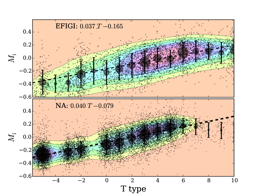
Figure 5.— The relationship between the morphological T-type and the morphometrix index $M_{\rm i}$ for EFIGI (above) and NA (below) databases. Small solid dots are individual galaxies; large circles indicate mean $M_{\rm i}$ for each integer T-type and their size is proportional to number of object; error bars indicate standard deviation in $M_{\rm i}$. Contours are draw for a kernel representation of points. The dashed line are the best linear regression, whose parameters are shown on top of each plot.

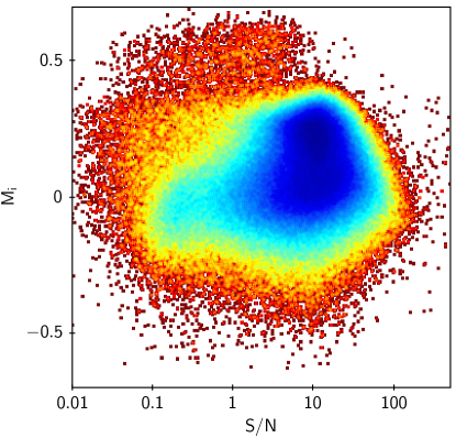
Figure 6.— Comparison between the signal-to-noise of the galaxy defined as S/N$=I_{n,2D}$/skybgstd and the Morphometric Index M_i.

8. Comparison with other physical parameters

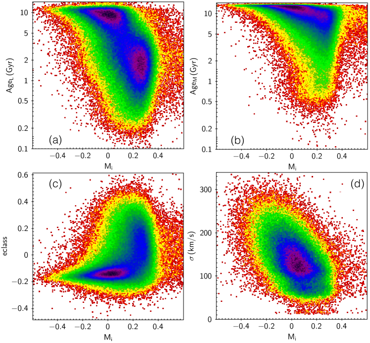
Figure 7.— Relationship between M_i and Age_L (age weighted by luminosity), Age_M (age weighted by mass), eClass and central velocity dispersion $\sigma$

We present in this paper a new approach for galaxy morphological classification that is not focused on recovering visual classification, although this is done remarkably well (see Section 6.3). In this work, the parameters defining the morphology of a galaxy are physically motivated and to confirm how successful we were in reaching this goal we compare $M_{\rm{i}}$ with quantities measured from the spectrum of the galaxies we measured.

Figure 7 exhibits how Age_L (age weighted by luminosity), Age_M (age weighted by mass), eClass (a single parameter classifier based on PCA analysis, retrieved from the SDSS database), and central velocity dispersion $\sigma$ correlate with $M_{\rm{i}}$. Notice that the SDSS spectra reflect properties of the central region of galaxies. In Figure 7.a we see that, overall, negative $M_{\rm{i}}$ corresponds to older systems. Age_L reflects more recent episodes of star formation and in this case as $M_{\rm{i}}$ goes to very negative the systems do not present any recent star formation, namely these are very old galaxies. There is a ridge of old systems extending from $M_{\rm{i}}$ = -0.5 up to 0.1 and then a significant drop in age as $M_{\rm{i}}$ tends to 0.2. For $0.1<M_{\rm{i}}<0.4$ we see that Age_L is around 1.5 Gyr. These are the late type spirals which exhibit a considerable amount of star formation. This figure clearly shows that morphology, in this case manifested by the parameter $M_{\rm{i}}$, varies continuously from old to young stellar population which is an important aspect of any morphological quantifier – to reflect stellar population properties of galaxies.

Figure 7.b is similar to Figure 7.a but plotting Age_M instead, which contrary to Age_L, reflects more the whole star formation history of a galaxy. The same trend is seen here, however since the SDSS spectra samples only the central region of the galaxies, there is a population that dominates the figure for Age_M around 10.0 Gyr, from early (negative $M_{\rm{i}}$) to late types (positive $M_{\rm{i}}$).

Figure 7.c exhibits how $M_{\rm{i}}$ is related to eClass, a parameter designed to express differences in stellar populations among different galaxies and then serving as a discriminant between early and late type systems. We find that the relation between these two quantities is not linear, which is what we would expect if both reflected morphology in a one-to-one relationship. What we see is that for $-0.5<M_{\rm{i}}<0.2$ eClass is concentrated around -0.15 (early type systems), with a scatter that increases as $M_{\rm{i}}$ increases. Then for $M_{\rm{i}}>0.2$ eClass increases steadily reaching eclass of 0.5 for $0.2<M_{\rm{i}}<0.4$. Both eClass and $M_{\rm i}$ are associated to morphology, although eClass is primarily associated with stellar population and $M_{\rm i}$ is derived solely based on image morphometry. $M_{\rm i}$ is more sensitive to morphology, particularly in the early-type systems domain ($M_{\rm i}<0$).

Finally, in Figure 7.d we present the relation with the central velocity dispersion $\sigma$ (corrected for an aperture of $R_{e}/8$, where $R_{e}$ is the effective radius of the galaxy). Even though with a large scatter a clear relation exists between $M_{\rm{i}}$ and $\sigma$, which is remarkable considering that $M_{\rm{i}}$ is solely photometric. In summary, these comparisons show that $M_{\rm{i}}$ is reliable in separating the different morphological types according to their stellar population properties, a performance not seen in other previously proposed morphological quantifiers.

9. Summary

We present a new method to establish morphological classification of galaxies that is physically motivated although it matches what is done visually for the very nearby Universe equally well. In the following, we summarize the main aspects of the classification system proposed here and the verification analysis:

1 - We developed a pipeline that automatically estimates morphometric parameters from galaxy images. Measured parameters include Concentration, $C_{1}$, Asymmetry, $A_{3}$, and Smoothness, $S_{3}$ which were slightly modified with respect to the conventional ones. We also make use of two new extra parameters: entropy $H$ and spirality $\sigma_{\psi}$.

2 - Morfometryka measures several quantities per galaxy which brings the question of which ones are more adequate for establishing the morphological type of the system. We use a method called Maximum Information Content (MIC) to select the relevant features avoiding redundancy. The new introduced morphometric parameters have a better discriminant power than previously used ones. MIC analysis resulted in the minimum number of independent parameters listed in item 1. The relationship between concentration, Petrosian radius and Sérsic index $n$ is derived in Appendix C and B.

3 - Our supervised classification is based on Galaxy Zoo and tested with different datasets: EFIGI, NA, LEGACY and LEGACY–$zr$. The Linear Discriminant Analysis (LDA) method is used to determine the decision surface that separates early from late type systems and the distance from this surface will indicate how early or late the system is. It is exactly this distance that we propose as a morphological index, $M_{\rm{i}}$.

4 - Classification performance was evaluated using the confusion matrix, from which we measured accuracy, precision and sensitivity scores, with a 10-fold cross validation scheme. We obtain final scores better than 90%.

5 - Another independent validation comes from comparing $M_{\rm{i}}$ with stellar population quantities and velocity dispersion which were established using the spectra available in DR7 together with the spectral fitting code starlight. We note that $M_{\rm{i}}$ correlates with eClass and it shows that classifying early-type galaxies solely as eClass $<0$ can significantly contaminate the sample with late-type systems which have $M_{\rm{i}}>0.2$.

Appendix A Morfometryka Algorithm Details

Here, we provide a detailed description of the various measurements in Morfometryka. mfmtk is logically divided into four main blocks (classes in programming parlance): Stamp – basic data reading and low level, low complexity geometrical measurements; Photometry –  luminosity distribution, star masking and Petrosian radius estimation; Sérsic – 1D and 2D luminosity distribution fitting; Morphometry – measurements of the morphometric parameters used later on for establishing the galaxy’s morphology. The package also include auxiliary applications makemySDSS for retrieving SDSS frames and cutting stamps and LDAclassify to perform the Linear Discriminant Analysis. In the following, logical units are written in small caps, algorithm code in typewriter.

A.1. Cutting stamps

The list of all objects, containing ObjIDs, RA, DEC, run, rerun, camcol, field and petroRad, is generated with the following SQL query on SDSS CasJobs

Ψ
SELECTΨp.objID, p.ra, p.dec, p.run, p.rerun, p.camcol, p.field, p.petroRad_r
ΨFROM DR7.SpecObj as s JOIN DR7.PhotoObj AS p ON s.bestObjID = p.objID
ΨWHERE s.specclass = 2.Ψ

From this list, we build a set of unique combinations of (run,rerun,camcol,field) and the required SDSS Frames and psFields are downloaded. We do it exactly as for DR7 Frames and psFields but we download the DR10 files since they refer to the same region of the sky, i.e. the raw data are the same, but the image processing algorithms were improved from DR7 to DR10. Also, DR10 frames are calibrated in nanomaggies (Lupton et al., 1999). For each object, the relative Frame is loaded and a square region of size 10 petroRad_r centered in the object’s RA and DEC is cut. The PSF for the same position is generated with the SDSS read_PSF application from the psField file. The stamp FITS file header is updated with the astrometry and relevant frame keywords. If the object is in the frame border, i.e., if it has less than 90% of pixels in the frame, a FITS header keyword FLAGINC and a header comment ”MFMTK: incomplete stamp” is written.

A.2. Basic image processing

The process starts with the target image gal0 and the associated PSF, which is measured from the second moment collapsed in the $y$ direction.The sky background skybg is estimated from the median of all pixels from the four corners of the image (squares of typical width of 10 pixels, skyboxsz). The accuracy of the sky background estimate skybgstd is set by the standard deviation of the aforementioned set of pixels.

The segmentation is done on the gal0fltr image, which is the gal0 image median filtered with a window of size segS (typically 5 pixels); high frequencies are filtered from the image to avoid sharp edges in the segmented regions. Regions are then selected by histogram thresholding: those pixels whose intensity are greater than the threshold median(gal0fltr)+segK$\cdot$ mad(gal0fltr) are selected, where mad is the median absolute deviation. This threshold selects segK mad above the median, which is similar to sigma-clipping $K$ standard deviations above the mean, except that median and the median absolute deviation (mad) are used, which are more robust to outliers and intensity variations. This histogram thresholding operates on the intensity space only and may select regions that are not spatially connected. The spatial information is taken into account by performing a connected-component labeling, where 4–connected pixels receive the same label. At this stage the segmentation consists of one or more labelled regions. The final segmented region is then selected either by size (largest) or by position (center of light closest to image center), depending on configuration. For SDSS stamps the position criteria is used. A segmentation mask segmask is made from the selected region, from which a segmented galaxy image gal0seg is derived; on both, pixels outside the segmentation region are nil. Geometric measurements in this section are done in the gal0seg image.

The galaxy image center is estimated in two distinct ways. First, the peak center $(x_{0},y_{0})_{\rm peak}$, referring to the locus where the intensity is maximum, is estimated from the center of light (first moment) of the 5$\times$5 matrix around the pixel with highest intensity, attainning sub-pixel precision.

For an image $I(x,y)$ the standard image moments are defined as

$$m_{pq}=\int\limits_{-\infty}^{\infty}\int\limits_{-\infty}^{\infty}x^{p}y^{q}I(x,y)\,dx\,dy,$$

and the center of light (CoL) $(x_{0},y_{0})_{CoL}$ are given by $x_{0}=m_{10}/m_{00}$ and $y_{0}=m_{01}/m_{00}$. The translational invariant moments $\mu_{pq}$ are determined by replacing $x$ and $y$ by $(x-x_{0})$ and $(y-y0)$, respectively, in $m_{pq}$. The axis lengths are given by

$$\lambda_{1}=\frac{\sqrt{|\mu_{20}+\mu_{02}+\Lambda|}}{m_{00}}\qquad\lambda_{2}=\frac{\sqrt{|\mu_{20}+\mu_{02}-\Lambda|}}{m_{00}}$$ (A1)

$$\text{where}\qquad\Lambda=\sqrt{(\mu_{20}-\mu_{02})^{2}+4\mu_{11}^{2}}$$ (A2)

from which we define

$$a=\max{(\lambda_{1},\lambda_{2})}$$

$$b=\min{(\lambda_{1},\lambda_{2})}.$$

Further, we can calculate the position angle of the main axis by

$$PA=\frac{1}{2}\ \arctan(2\mu_{11},\mu_{20}-\mu_{02}).$$

Details of the derivation of the relations above are given, for example, in (Flusser & Zitova, 2009).

For future use, a standardized version of the segmented galaxy image is calculated: given the parameters estimated above, an affine transform is applied to gal0seg such that in the resulting stangal image the object is centered in the image array, has zero position angle and its axial ratio is unity. Optionally the integrated luminosity can be normalized.

A.3. Photometry Routines

Photometry is performed by positioning successive ellipses relative to a fixed center $(x_{0},y_{0})_{\rm peak}$, with constant axis ratio $b/a$ and position angle $PA$. The photometric measurements are performed for ellipses with semi-major axis $R$ ranging from 1 pixel up to the size of the image diagonal, in steps of 1 pixel. Later the profiles are truncated (see below).

The pixels 1 pixel away from the ellipse are called border pixels (ellindxbrdr) and the pixels inside the ellipse are internal pixels (ellindxin). In a given semi-major axis $R$, for the set of border pixels, those pixels whose intensity are above some threshold relative to the pixel group (given by median(ellindxbrdr)+StarSigma$\cdot$mad(ellindxbrdr)) are masked as stars. The ellipse mean intensity $I(R)$ and associated error $I_{\mathrm{err}}(R)$ are calculated by the average and the standard deviation of the border pixels not masked as stars. The total luminosity $L(R)$ is the sum of the internal pixels for each ellipse, and the mean intensity $\langle I\rangle(R)$ is given by the ratio of $L(R)$ and the number of pixels inside the ellipse.

At each semi-major axis iteration, the Petrosian function, Eq.(A6), is evaluated and once it falls below the critical value $\eta_{0}=5$, the Petrosian radius $R_{p}$ is evaluated by linear interpolating $\eta(R)$ between the adjacent points. A Petrosian Region is defined as an elliptic region of semi-major axis $N_{\!R_{p}}\cdot R_{p}$ (we use $N_{\!R_{p}}=2$) and the same axis-ratio and position angle measure in the segmented image (Section A.2), and stored as petromask. The image galpetro = petromask $\cdot$ gal0 is defined. The profiles $I(R)$, $I_{\rm err}$, $L(R)$ and $\langle I\rangle(R)$ are cut at $N_{\!R_{p}}\cdot R_{p}$.

A.4. The Sérsic routines

Standard 1D Sérsic parameters are measured by fitting the Sérsic law (Sersic, 1967)

$$I(R)=I_{n}\exp\left[-b_{n}\left(\frac{R}{R_{n}}\right)^{{}^{1}/_{n}}-1\right]\quad\text{with}\quad b_{n}=2n-\frac{1}{3},$$ (A3)

to the 1D surface brightness profile $I(R)$. The minimizations are done with a Levenberg-Marquardt algorithm, in a least squared sense. The fits are bounded by adding a square penalty function for parameters outside the specified range. The boundaries are: $\min[I(R)]<I_{n,1D}<\max[I(R)]$, $1<R_{n,1D}<\max[R]$, $\frac{1}{2}<n_{1D}<50$. The output parameters are $I_{n,1D}$, $R_{n,1D}$, $n_{1D}$.

The 2D fitting applies Eq. (A3) convolved with the PSF and with $R$ replaced by $R=\sqrt{x^{\prime 2}+y^{\prime 2}/q_{2D}^{2}}$, where

$$x^{\prime}=\ (x-x_{0}^{2\!D})\cos(PA^{2\!D})-(y-y_{0}^{2\!D})\sin(PA^{2\!D})$$ (A4)

$$y^{\prime}=-(x-x_{0}^{2\!D})\sin(PA^{2\!D})-(y-y_{0}^{2\!D})\cos(PA^{2\!D}).$$ (A5)

Coordinates $x,y$ refers positions in the galaxy image. The two-dimensional Sérsic function is fitted directly to the galaxy image, except that pixels outside the galaxy, as defined by the Petrosian Region, flagged stars and central circular region of 1 PSF FWHM are masked. The algorithm is the same as for 1D fitting, with the following boundaries: the center $(x_{0},y_{0})_{2D}$ cannot vary more than 15% compared to $(x_{0},y_{0})_{\rm peak}$; $I_{n,2D}$ must be within image pixel values range; $R_{n,2D}$ cannot be greater than the image half-diagonal; $\frac{1}{2}<n_{2D}<20$, $\frac{1}{10}<q_{2D}=b/a<1$. This setup has proven in simulation and in real galaxies to be the most stable, converging for most galaxies in the samples. The fit free parameters are $\{x_{0},y_{0},PA,q,I_{n},R_{n},n\}_{2D}$.

Based on simulations of synthetic Sérsic galaxies, we found that the 2D fitting is better than 1D at recovering ”true” parameters from images. Since the 2D is more unstable to initial parameters, we use the 1D results as the initial guess for the 2D fit.

A.5. Quality Flags

For reference, a series of conditions are evaluated and informative Quality Flags (QF) are saved. They are not conclusive but may indicate situations when the condition occur. For example, if for a given object the $R_{n,2D}$ is of the order of the PSF, $n_{2D}\sim 0.5$ (a Gaussian) and $b/a\sim 1$, the object is probably a star, a Morfometryka target selection error. Other QF indicate that the fitting routine did not converge in situations of a crowded field. For detecting crowded fields, we define the asymmetry $A_{4}$ as the distance between $\mathbf{r}_{\rm CoL}=(x_{0},y_{0})_{\rm CoL}$ and $\mathbf{r}_{\rm peak}=(x_{0},y_{0})_{\rm peak}$ in units of $R_{p}$, in percentage,

$$A_{4}=100\frac{\textbf{r}_{\rm CoL}-\textbf{r}_{\rm peak}}{R_{p}},$$

which attains values greater than $\sim 10$ in crowded fields, and is used to turn the QF64 on.

The QF are summarized in Table 3.

Flag	NAME	DEC	HEX	CRITERIA
QF0	normal	0	0x00	no unusual situation
QF1	targetsize	1	0x01	psf_fwhm $>R_{p}$
QF2	targetisstar	2	0x02	$R_{n,2D}\leq\mathtt{psf\_fwhm}$ and $n_{2D}\leq 0.55$ and $b/a>0.8$
QF4	fit1Derror	4	0x04	1D fitting routine did not converge
QF8	fit2Derror	8	0x08	2D fitting routine did not converge
QF16	crowded1	16	0x10	more than 5% of Petro region masked as stars
QF32	crowded2	32	0x20	$R_{n,2D}>2R_{p}$
QF64	crowded3	64	0x40	$A_{4}>10$

Table 3Morfometryka quality flags used that mark unusual situations

A.6. Petrosian Quantities

Petrosian (1976) defined a function $\eta(R)$ which is the ratio of the mean intensity inside $R$ to the intensity at the isophote $R$

$$\eta(R)=\frac{\langle I\rangle(R)}{I(R)}.$$ (A6)

The Petrosian radius is the distance from the galaxy center where the fraction in Eq.(A6) has some constant value

$$\eta(R_{p})=\eta_{0}.$$

Here we use $\eta_{0}=5$. The virtue of $\eta$ is that both the numerator and denominator have the same dependence with the distance, hence $\eta$ is distance independent. The Petrosian radius is used as a implicit scale length for each galaxy.

Appendix B Petrosian radius and Sérsic index equivalence

The mean intensity within radius $R$ for a Sérsic model is the integrated luminosity up to $R$ divided by the region area $\langle I\rangle=L(R)/A$, $A=\pi R^{2}$, so for $x\equiv b_{n}(R/R_{n})^{1/n}$, we have (see for example Ciotti & Bertin (1999); Graham & Driver (2005))

$$\langle I\rangle(R)=2n\,I_{n}\,e^{b}\;\frac{\gamma(2n,x)}{x^{2n}}.$$ (B1)

We then have for the Petrosian function Eq. A6

$$\eta(R)=\frac{2n\gamma(2n,x)}{x^{2n}e^{-x}}.$$ (B2)

We have to solve

$$\frac{2n\gamma(2n,x_{p})}{x_{p}^{2n}e^{-x_{p}}}=\eta_{0}\quad\text{with}\quad x_{p}=x(R_{p}),$$ (B3)

to obtain $R_{p}$ as a function of $n$. This equation is transcendental and can only be solved for $R_{p}$ numerically. However, for practical purposes, we can write an empirical Petrosian Radius function

$$R_{p}(n)=R_{n}\;R_{p}^{\rm max}\ \frac{n-n_{0}}{a}\exp\left[-\left(\frac{n-n_{0}}{a}\right)^{\alpha}\right]$$ (B4)

whose parameters $R_{\rm max}=5.8$, $n_{0}=-1.11$, $a=2.04$ and $\alpha=0.8$ provide a fit better than 1% over the range $0.3<n<15$, as shown in Figure 8.

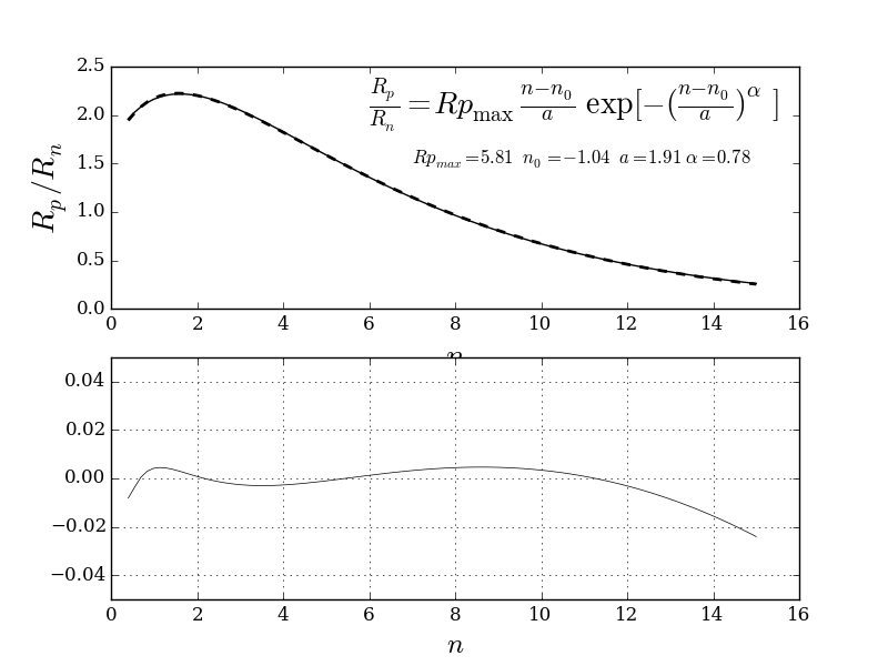
Figure 8.— Petrosian radius as a function of $n$. Top: numerical (dashed) and empirical function (continuous). Bottom: fractional error between the two.

Appendix C Concentration and Sérsic index equivalence

In the case of Sérsic law, the integrated luminosity within radius $R$ (Ciotti & Bertin, 1999) is

$$L(R)=2\pi n\,I_{n}R_{n}^{2}\,\frac{e^{b}}{b^{2n}}\;\gamma(2n,x)$$ (C1)

with $x\equiv b_{n}(R/R_{n})^{1/n}$. Hence the total Luminosity $L_{T}=L(R\to\infty)$ is

$$L_{T}=2\pi n\,I_{n}R_{n}^{2}\,\frac{e^{b}}{b^{2n}}\;\Gamma(2n).$$ (C2)

From Eqs. C1 and C2 we have the equation for the $R_{f}$ which attains some fraction $f$ of the total luminosity

$$\gamma(2n,x_{f})=f\ \Gamma(2n)\qquad\textrm{with}\qquad x_{f}=x(R=R_{f})$$ (C3)

or for both $R_{f1}$ and $R_{f2}$

$$\frac{\gamma(2n,x_{f1})}{\gamma(2n,x_{f2})}=\frac{f_{1}}{f_{2}}$$ (C4)

Equation (C4) cannot be solved analytically (except for $n=1/2$) and the solution must be found numerically. Figure 9 shows the numerical solution for $1/2<n<15$.

Again, we can write an empirical function

$$C(n)=C^{\prime}\left(\frac{n}{n^{\prime}}\right)^{\beta}$$ (C5)

which approximates the solution in the specified range with an error smaller than 2% for $C_{1}$ in the range $1<n<15$, with $C^{\prime}=2.91$, $n^{\prime}=32.44$ and $\beta=0.48$

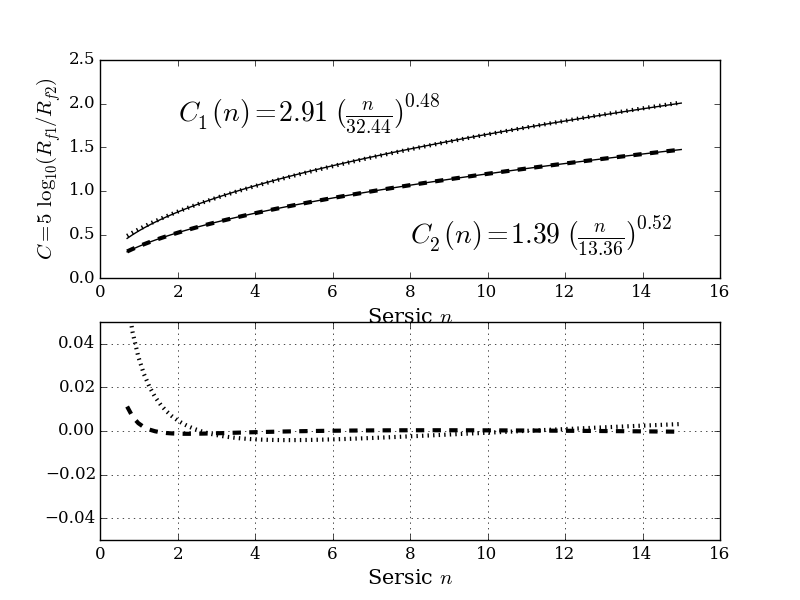
Figure 9.— Concentration as a function of $n$. Top: numerical (dotted for $C_{1}$, dashed for $C_{2}$) and empirical function (continuous). Bottom: fractional error between the two.

Appendix D Histogram of Morphometric Parameters for Databases

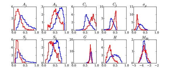
Figure 10.— Distribution of feature values among morphometric classes for the EFIGI database.

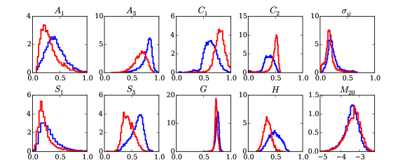
Figure 11.— Distribution of feature values among morphometric classes for the NA database.

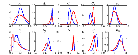
Figure 12.— Distribution of feature values among morphometric classes for the LEGACY complete sample.

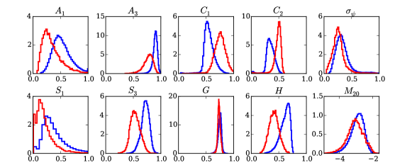
Figure 13.— Distribution of feature values among morphometric classes for the LEGACY–$zr$ sample.

References

- Abazajian et al. (2009) Abazajian, K. N., Adelman-McCarthy, J. K., Agüeros, M. A., et al. 2009, ApJS, 182, 543
- Abraham et al. (1994) Abraham, R. G., Valdes, F., Yee, H. K. C., & van den Bergh, S. 1994, ApJ, 432, 75
- Abraham et al. (1996) Abraham, R. G., van den Bergh, S., Glazebrook, K., et al. 1996, ApJS, 107, 1
- Albanese et al. (2013) Albanese, M. F., Visintainer, R., Riccadonna, S., et al. 2013, Bioinformatics, 29, 407.
- Andrae et al. (2011) Andrae, R., Jahnke, K., & Melchior, P. 2011, MNRAS, 411, 385
- Baillard et al. (2011) Baillard, A., Bertin, E., de Lapparent, V., et al. 2011, A&A, 532, A74
- Bershady et al. (2000) Bershady, M. A., Jangren, A., & Conselice, C. J. 2000, AJ, 119, 2645
- Bishop (2007) Bishop, C.M. 2007. Pattern Recognition and Machine Learning, Springer. ISBN-13 978-0387310732.
- Cardelli et al. (1989) Cardelli, J. A. and Clayton, G. C. and Mathis, J. S., 1989, ApJ, 345, 245
- Cid Fernandes et al. (2005) Cid Fernandes, R., Mateus, A., Sodré, L., Stasińska, G., & Gomes, J. M. 2005, MNRAS, 358, 363
- Ciotti & Bertin (1999) Ciotti, L., & Bertin, G. 1999, A&A, 352, 447
- Conselice et al. (2000) Conselice, C. J., Bershady, M. A., & Jangren, A. 2000, ApJ, 529, 886
- de Vaucouleurs (1959) de Vaucouleurs, G., Handbuch der Physik, 1959, Vol. 53, pp. 275-310
- de Vaucouleurs et al. (1991) de Vaucouleurs G., de Vaucouleurs A., Corwin H. G., Jr, Buta R. J., Paturel G., Fouqué P., 1991, Third Reference Catalogue of Bright Galaxies. Springer, New York, NY
- Dieleman et al. (2015) Dieleman, S., Willett, K. W., & Dambre, J. 2015, MNRAS, 450, 1441
- Duda (2001) Duda, R., Hart, P.E., Stork, D.G. 2000. Pattern Classification (2nd ed.). Wiley-Interscience, ISBN-13 978-0471056690.
- Falcón-Barroso et al. (2011) Falcón-Barroso, J., Sánchez-Blázquez, P., Vazdekis, A., et al. 2011, A&A, 532, A95
- Fasano et al. (2012) Fasano, G., Vanzella, E., Dressler, A., et al. 2012, MNRAS, 420, 926
- Flusser & Zitova (2009) Flusser, J., Zitova, B., Suk, T., 2009, Moments and Moment Invariants in Pattern Recognition. Wiley, ISNBN-13 978-0470699874.
- Freeman et al. (2013) Freeman, P. E., Izbicki, R., Lee, A. B., et al. 2013, MNRAS, 434, 282
- Girardi et al. (2000) Girardi, L., Bressan, A., Bertelli, G., & Chiosi, C. 2000, A&AS, 141, 371
- Graham & Driver (2005) Graham, A. W., & Driver, S. P. 2005, PASA, 22, 118
- Gunn & Gott (1972) Gunn, J. E., & Gott, J. R., III 1972, ApJ, 176, 1
- Hackeling (2014) Hackeling, G. 2014, Mastering Machine Learning With Scikit-Learn, Packt Publishing. ISBN-13 978-1783988365.
- Hamming (1998) Hamming, R. W., 1998. Digital Filters (3rd ed.). Courier Dover Publications. ISBN-13 978-0486650883.
- Hubble (1926) Hubble, E. P. 1926, ApJ, 64, 321