BAT AGN spectroscopic survey II: X-ray emission and high ionization optical emission lines

Abstract

We investigate the relationship between X-ray and optical line emission in 340 nearby ($z\simeq 0.04$) AGN selected above 10 keV using Swift BAT. We find a weak correlation between the extinction corrected [O iii] and hard X-ray luminosity ($L_{\left[{\rm O}\,\textsc{iii}\right]}^{int}\propto L_{14-195}$) with a large scatter ($\rm{R_{Pear}=0.64}$, $\rm{\sigma=0.62}$ dex) and a similarly large scatter with the intrinsic 2$-$10 keV to [O iii] luminosities ($\rm{R_{Pear}=0.63}$, $\rm{\sigma=0.63}$ dex). Correlations of the hard X-ray fluxes with the fluxes of high-ionization narrow lines ([O iii], He ii, [Ne iii] and [Ne v]) are not significantly better than with the low ionization lines (H$\alpha$, [S ii]). Factors like obscuration or physical slit size are not found to be a significant part of the large scatter. In contrast, the optical emission lines show much better correlations with each other ($\sigma=0.3$ dex) than with the X-ray flux. The inherent large scatter questions the common usage of narrow emission lines as AGN bolometric luminosity indicators and suggests that other issues such as geometrical differences in the scattering of the ionized gas or long term AGN variability are important.

1 Introduction

Based on the unification model of active galactic nuclei (AGN; Urry et al., 1991; Antonucci, 1993; Urry & Padovani, 1995), narrow optical emission lines are emitted from the narrow-line region (NLR). The NLR is ionized by the Extreme UV–soft X-ray emission from the AGN’s central engine. Afterwards, the illuminated interstellar gas in the NLR radiatively cools down by emitting the narrow optical lines. Unlike this optical emission, X-rays are emitted from much closer to the supermassive black hole (SMBH). The UV photons radiated by the accretion disk are inverse Compton scattered inside the corona and can reach energies up to a few hundreds of keV (e.g., Netzer, 2013). Thus, if AGN are accreting at a constant rate and constantly ionizing the NLR, we would naively expect a tight correlation between the X-ray emission from the corona and the optical emission lines from the NLR. This is why both high ionization optical emission lines and X-rays are thought to be reliable tracers of the AGN bolometric luminosity ($L_{bol}$) and of the black hole growth (Heckman et al., 2005).

The bolometric luminosity ($L_{bol}$) of unobscured AGN estimated from the spectral energy distribution (SED) fitting technique using optical, UV, and X-ray data shows a tight correlation with hard X-ray data alone (e.g., 14$-$195 keV with a scatter of 0.3 dex, Vasudevan et al., 2009) though X-ray surveys may not detect heavily obscured Compton-thick AGN ($N_{\rm H}>10^{24}$ cm^-2). Strong observational correlation has also been found between UV emission and X-ray emission (Steffen et al., 2006; Young et al., 2010). The use of [O iii] $\lambda 5007$ to infer AGN bolometric luminosities has a long history (e.g., Heckman et al., 2004; LaMassa et al., 2009; Kauffmann & Heckman, 2009). It has been widely used to estimate the accretion rates of AGN using bolometric corrections based on the X-ray emission, the 5100 Å monochromatic continuum or the mid-IR emission (e.g., Lamastra et al., 2009). However, several studies have noted that the strength of [O iii] $\lambda 5007$ is modulated by factors including covering factor of the narrow-line region gas and its density (e.g., Netzer & Laor, 1993), and ionization parameter (e.g., Baskin & Laor, 2005).

Previous studies have compared X-ray emission with optical emission lines strengths in hard X-ray selected samples. Heckman et al. (2005) used a sample of 47 local AGN ($z<$0.2) from the RXTE slew survey to analyze the correlation between 3-20 keV flux and the [O iii] strength (Revnivtsev et al., 2004; Sazonov & Revnivtsev, 2004). Other works have also made use of the early results from the Swift BAT survey (9-month catalog, Tueller et al., 2008) to analyze optical and X-ray emission from AGN. Meléndez et al. (2008) studied the correlation between the [O iii] $\lambda 5007$ line strength and two X-ray bands (2$-$10 keV and 14$-$195 keV) for 40 low redshift (z$<$0.08) BAT AGN from the 9-month catalog. Winter et al. (2010) made a similar analysis with a slightly larger sample (64 BAT AGN). Finally, an analysis of the full 9-month catalog has recently been completed ($\approx$100 BAT AGN, Ueda et al. 2015, submitted). Netzer et al. (2006) studied a sample of 52 obscured AGN at high redshift ($z\approx$1) suggesting that [O iii] emission is weaker relative to 2$-$10 keV emission in high $L_{X}$ sources.

The Swift BAT 70-month all-sky survey enables us to analyze the optical and X-ray properties of a large sample of nearby AGN. It has detected 823 AGN to a flux limit of $\approx 10^{-11}\ \mathrm{erg\ cm^{-2}\ s^{-1}}$ over the whole sky (Baumgartner et al., 2013). Due to its detection method in the ultra hard X-rays (14$-$195 keV), the Swift BAT survey is not affected by obscuration (below Compton-thick levels) nor is it contaminated by stellar emission. Therefore, it also includes ’buried’ obscured AGN that may not have been selected by optical surveys (e.g., Ueda et al., 2007).

In this work, we use a sample of BAT AGN based on the 70-month catalog with an optical spectroscopic sample that is significantly larger than previous studies (340 objects). Our spectroscopic analysis also includes higher ionization lines not used previously (i.e., [Ne v]$\,\lambda 3426$) to study correlations between optical line emission and X-ray emission. The sample is presented in Section 2 and our analysis methods are described in Section 3. We study the correlation between [O iii] and X-ray emission in Section 4.1, X-ray and other high ionization lines (i.e., [Ne iii] $\lambda 3869$, He ii $\lambda 4686$, and [Ne v]$\,\lambda 3426$) in Section 4.2, and the correlation between only optical emission lines in Section 4.3. Finally, a review of our results and a discussion is presented in Section 5.

2 Sample

The optical data are taken from the BAT AGN Spectroscopic Survey (BASS) Data Release 1 (Koss et al., in prep.), which gathered 559 optical spectra from targeted spectroscopic campaigns on BAT sources and public optical surveys (SDSS and 6DF, Alam et al., 2015; Jones et al., 2009). This sample is the largest and the most complete catalog of AGN optical spectra selected from the Swift  hard X-ray survey. It contains 67.6% of the total AGN detections in the Swift BAT 70-month catalog and has a mean redshift of $z=0.10$.

From this parent sample, we first remove the spectra coming from the 6dF survey because they lack flux calibration. We remove all blazars listed in the Roma blazar catalog (BZCAT) v5.0 (Massaro et al., 2009) since the X-ray emission in such sources is affected by differential beaming. We also apply two redshift cuts. The first one, $z>0.01$, avoids very nearby star-forming galaxies (such as M82) and ensures that a significantly large portion of the ionized region within the galaxy is covered (i.e., $>$0.2  kpc). We also limit to $z<0.4$ to avoid redder emission lines such as H$\alpha$ from being shifted outside the observed wavelength interval. Additionally, we remove ten spectra due to calibration problems around the [O iii] line. Finally, we exclude SDSS J155334.73+261441.4, a gravitationally lensed quasar (Ofek et al., 2007). The final sample totals 340 optical spectra with $\langle z\rangle=0.05$.

We define an emission line detection when we reach a SNR$>$3 of the line with respect to the noise of the adjacent continuum. Out of these 340 objects, we have 327 detections of [O iii], 301 of H$\alpha$, 281 of [N ii], 278 of [S ii], 265 of H$\beta$, 206 of [O i], 144 of [Ne iii], 106 of He ii and 51 of [Ne v]. The intrinsic 2$-$10 keV flux values and the column density measurements provided for 335/340 AGN are based on a homogeneous model fitting using the best available X-ray data with simultaneous modeling of the 0.2$-$10 keV band from XMM-Newton, Chandra, or Swift XRT and the 14$-$195 keV band from Swift BAT (details in Ricci et al., in prep).

We use the AGN emission-line diagnostics (e.g., Baldwin et al., 1981; Veilleux & Osterbrock, 1987) as updated by Kewley et al. (2006) to further classify our sample. We classify as low ionization nuclear emission-line region (LINER) any object that shows a LINER classification in either the [O i]$\,\lambda 6300$ or [S ii]$\,\lambda 6717,6731$ diagnostic. For the remaining AGN, we use the [N ii]$\,\lambda 6583$ diagnostic, which is most sensitive to AGN, to differentiate between Seyfert AGN and HII/composite/ambiguous (17/340). We use the presence of a broad line in H$\alpha$ to differentiate between type 1 (217/340) and type 2 objects (116/340). A more detailed description of the reduction procedures of the optical spectra, sample selection, and overall properties of the optical spectroscopic sample can be found in the BASS-I paper (Koss et al., in prep).

3 Analysis of optical spectra

We fit our sample of optical spectra using an extensive spectroscopic analysis toolkit for astronomy, PySpecKit, which uses a Levenberg-Marquardt algorithm for fitting (Ginsburg & Mirocha, 2011). We implement separate methods for fitting sources with narrow lines only and sources with broad lines. We fit the H$\beta$ (4650-5050 Å), H$\alpha$ (6250-6770 Å), and [O ii] (3300-4000 Å) spectral regions separately. For narrow-line sources, we first fit the spectrum with stellar templates using the pPXF software (Penalized PiXel Fitting; Cappellari & Emsellem, 2004) to remove the galaxy continuum and stellar absorption features that can effect line measurements. All emission line fits were inspected by eye to verify proper fitting.

We adopt a power-law fit (1st order) to model the continuum and Gaussian components to model the emission lines for different spectral regions. For the H$\alpha$ spectral region, we fit the [O i]$\,\lambda 6300$, [N ii] $\lambda 6548$, H$\alpha$, [N ii]$\,\lambda 6583$, and [S ii] $\lambda 6716$, and [S ii] $\lambda 6731$ lines. The narrow-line widths are tied together with an allowed variation of $\pm$ 8 Å and the systemic redshift is determined from the H$\alpha$ line. The relative strengths of [N ii] $\lambda 6548$ and [N ii]$\,\lambda 6583$ lines are fixed (at 1:2.94). For the H$\beta$ spectral region, we fit the He ii $\lambda 4686$, H$\beta$, [O iii] $\lambda 4959$, and [O iii] $\lambda 5007$ lines. The narrow-line widths are also tied together with an allowed variation of $\pm$ 8 Å and their central wavelengths are defined by the redshift of [O iii] $\lambda 5007$. The intensity of [O iii] $\lambda 4959$ relative to [O iii] $\lambda 5007$ is fixed (at 1:2.86). For the [O ii] spectral region, we fit the [Ne v] $\lambda 3346$, [Ne v] $\lambda 3426$, [O ii] $\lambda 3727$, [Ne iii] $\lambda 3869$, and [Ne iii] $\lambda 3968$ lines.

Two Gaussian components are allowed for the H$\alpha$ and H$\beta$ emission lines: a narrow component (FWHM $<1000\ {\rm km\,s}^{-1}$) and a broad component (FWHM $>1000\ {\rm km\,s}^{-1}$). The broad H$\beta$ component is only allowed if a broad H$\alpha$ component is detected. In the case of a non-detection of the narrow H$\alpha$ or [S ii]$\,\lambda 6717,6731$ line (i.e., due to a very strong broad H$\alpha$ component, a noisy spectrum or bad sky subtraction), we use the FWHM of [O iii] $\lambda 5007$ to constrain the widths of the narrow lines in the H$\alpha$ region.

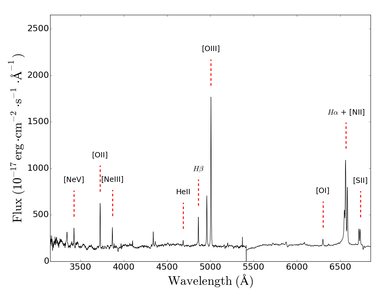
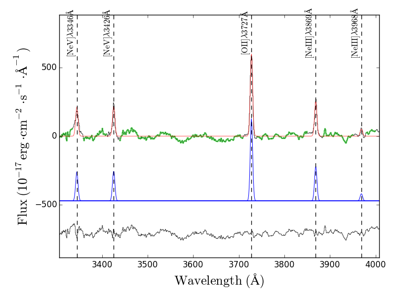
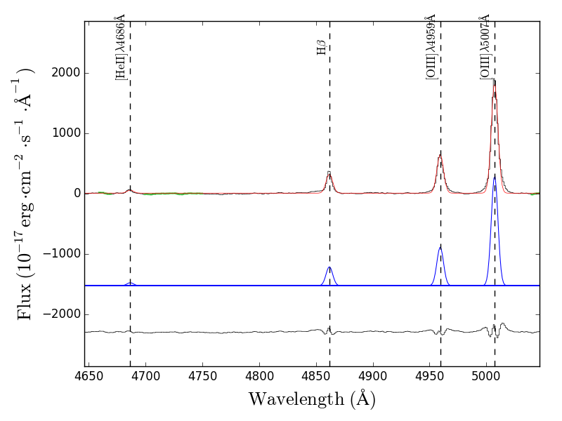
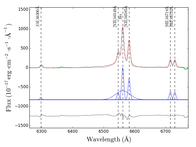
Figure 1: Example of the fitting procedure for MCG +06-16-28 observed with the Palomar Double Spectrograph. Top left panel: Spectrum of the object with all the fitted emission lines. Rest frame continuum subtracted fits are shown for the [O ii] (top right), H$\beta$ (bottom left), and H$\alpha$ (bottom right) spectral regions. The colors denote regions used for continuum (green), different Gaussian components of the fit (blue), and model fits (red) with residuals shown in the bottom panel.

To estimate the continuum for the H$\alpha$ complex, we use the wavelength regions 5800-6250 Å and 6750-7000 Å. For the H$\beta$ complex, we use the 4660-4750 Å (except around He ii) and 5040-5200 Å regions. The continuum around the [O ii] spectral region is usually more complicated to fit due to a non-linear shape or because it lies at the blue limit of the wavelength coverage. To fit this blue continuum, we use the region between 3300 Å and 4000 Å except where the emission lines are located ($\pm$ 15 Å). To estimate errors in line fluxes and line widths, we use a Monte Carlo simulation that adds noise based on the error spectrum and reruns the fitting procedure 10 times. The flux uncertainty for the [O iii] emission line is typically less than 1%. To correct our line ratios for dust extinction, we use the narrow Balmer line ratio (H$\alpha$/H$\beta$) assuming an intrinsic ratio of R=3.1 (e.g., Ferland & Osterbrock, 1986) and the Cardelli et al. (1989) reddening curve when both the narrow H$\alpha$ and H$\beta$ are detected. Figure 1 shows an example spectrum and best model fit.

4 Results

4.1 X-ray and [O iii] $\lambda 5007$ Flux

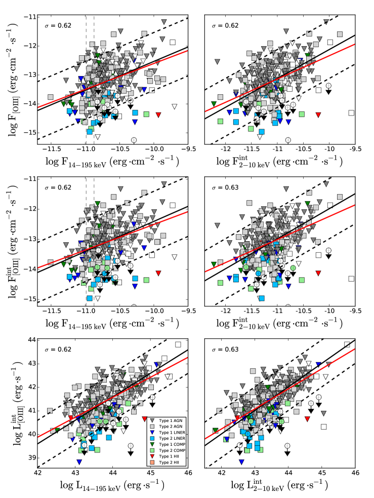
Figure 2: Plots of the relation of the [O iii] $\lambda 5007$ emission line strength with the BAT X-ray emission (left) and with the 2$-$10 keV emission (right). The [O iii]« – »X-ray relation exhibits a large scatter in all panels ($\approx$0.6 dex). The black solid lines show a fit constrained by $Y\propto X$ with the dashed lines showing the $\pm$1 dex. The red lines illustrate the linear regression. For both line fits we removed the four largest outliers. The color code comes from the the [N ii] BPT classification. White symbols do not have any BPT classification because of undetected emission lines. The AGN showing broad H$\alpha$ emission are classified as type 1. On the top and central left panels the grey dashed lines illustrate the 14$-$195 keV flux limits for 50% (left line) and 90% of the sky (right line). The upper limits were ignored in the analysis. Top panels: observed [O iii] flux plotted against the X-ray fluxes. Central panels: extinction corrected [O iii] flux plotted against the X-ray fluxes. Lower panels: extinction corrected [O iii] luminosity vs. the two X-ray luminosities.

We first compare the X-ray flux (2$-$10 keV and 14$-$195 keV) to the [O iii] $\lambda 5007$ emission line (Figure 2). The relation between the [O iii] corrected flux and the BAT X-ray flux shows a scatter of $\sigma$=0.62 dex and a Pearson correlation coefficient of $\rm{R_{Pear}=0.35}$. The result is very similar when comparing [O iii] to the 2$-$10 keV flux ($\sigma$=0.63, $\rm{R_{Pear}=0.38}$). The Pearson $p$-value representing the probability of the hypothesis to have no correlation at all between the two X-ray fluxes and the [O iii] flux is $<10^{-10}$ because of the large sample size. The correlation in luminosity space is better ($\rm{R_{Pear}^{14-195}=0.64}$, $\rm{R_{Pear}^{2-10}=0.63}$) than in flux space, as expected because the same multiplicative factor ($4\pi d_{L}^{2}$) is applied to both the X-ray flux and the [O iii] flux to obtain the luminosities. We finally compare the [O iii] $\lambda 5007$ flux both with ($F_{\left[{\rm O}\,\textsc{iii}\right]}^{int}$) and without ($F_{\left[{\rm O}\,\textsc{iii}\right]}$) extinction correction to the two X-ray band fluxes. We find no significant improvement in the scatter of the different relations ($\sim$0.01 dex) using the Balmer decrement corrected [O iii] fluxes.

Next, we compare a one-to-one relation and the linear regression in logarithmic space to fit our data. For both slope fits, we remove the four largest outliers. For the line fitting, we use the python routine scipy.optimize.curve_fit which provides a least squares approach (OLS(Y$\mid$ X)) with the Levenberg-Marquardt gradient method for convergence. The black solid lines in the panels of Figure 2 show the best one-to-one relation (which would imply that $L_{\left[{\rm O}\,\textsc{iii}\right]}^{int}\propto L_{14-195}$). The best fit for the linear regression, shown with the red lines, is $L_{\left[{\rm O}\,\textsc{iii}\right]}^{int}\propto(L_{14-195})^{0.85\pm 0.05}$ and $L_{\left[{\rm O}\,\textsc{iii}\right]}^{int}\propto(L_{2-10}^{int})^{0.85\pm 0.05}$. To test if the linear regression is a significantly better fit, we run a $F$-test. The $F$-test compares the sum of the residuals squared of two different models. We obtain a $F$-value of 7.66 for the 14$-$195 keV flux and of 7.81 for the 2$-$10 keV flux. The resulting $p$-values are lower than 1% suggesting that the linear regression between the [O iii] luminosity and the two X-ray bands is a significantly better model than a one-to-one relation. However, the improvement in the scatter is very small ($\approx$ 0.01 dex). Therefore, we decided to use the one-to-one relation (the simplest model) for the rest of the analysis.

We also use the Astronomy Survival Analysis (ASURV) package from the STATCODES suite of utilities developed by Eric Feigelson (Feigelson 1985). We determine the correlation between [O iii] and X-ray luminosity in the presence of the 13 upper limits in [O iii]. Specifically, we use the EM algorithm, though the Buckley James yields similar results. We find the best fit correlations is $L_{\left[{\rm O}\,\textsc{iii}\right]}^{int}\propto(L_{14-195})^{0.83\pm 0.06}$ which is consistent with the least squares approach suggesting the small number of non-detections do not significantly change the slope of the correlation.

Finally, we use the OLS bisector method of line fitting which is more reliable at recovering the intrinsic slope in the presence of uncertainties in both the X and Y variables (e.g. Isobe 1990). Table 1 lists the best fit linear regressions for the luminosity-luminosity plots using the OLS bisector method as well as the standard deviation for the complete sample and various sub-samples (Type 1-1.9, Type 2, Seyferts, LINERs, and HII/composite/ambiguous). The LINERS and HII/composite objects (from the BPT classification; Baldwin et al., 1981; Veilleux & Osterbrock, 1987) have on average lower X-ray and [O iii] luminosities than Seyfert galaxies: $\langle\log\ L_{\left[{\rm O}\,\textsc{iii}\right],int}^{LIN}\rangle=40.5$; $\langle\log\ L_{\left[{\rm O}\,\textsc{iii}\right],int}^{comp}\rangle=40.9$; $\langle\log\ L_{\left[{\rm O}\,\textsc{iii}\right],int}^{Sey}\rangle=41.5$.

4.1.1 Correlations with obscuration and luminosity

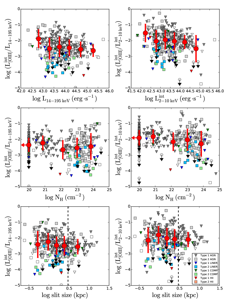
Figure 3: Plots of the $L_{\left[{\rm O}\,\textsc{iii}\right]}^{int}/L_{X}$ ratio as a function of X-ray luminosity (top panels), column density (central panels), and physical slit size (lower panels). The color codes represent the [N ii] BPT classification. White symbols do not have any BPT classification because of undetected emission lines. The red dots represent average binned values and the red bars show 1-sigma deviations in the bins. The first bin of the central panels represents a upper limit where the column density is consistent with the Galactic neutral hydrogen. The horizontal black lines on the lower panels illustrate the $3\ kpc$ value. The scatter increases for $N_{\rm H}>10^{22}$ cm^-2 with no change in average $L_{\left[{\rm O}\,\textsc{iii}\right]}^{int}/L_{X}$. For slit size, the scatter decreases with increasing slit size because of a higher fraction of unobscured AGN at higher redshifts, but the average $L_{\left[{\rm O}\,\textsc{iii}\right]}^{int}/L_{X}$ is constant. The upper limits were ignored in the analysis.

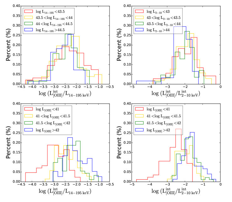
Figure 4: Histograms of the $L_{\left[{\rm O}\,\textsc{iii}\right]}^{int}/L_{X}$ ratio binned by X-ray luminosity (top panels) and [O iii] luminosity (lower panels). The two lower panels show a strong positive correlation of the ratio with the [O iii] luminosity.

The two upper panels of Figure 3 show the $L_{\left[{\rm O}\,\textsc{iii}\right]}^{int}/L_{X}$ ratio as a function of X-ray luminosity. The red dots show the average trend and the error bars the average 1-$\sigma$ scatter. First, we notice that there is no significant difference between the 2$-$10 keV (right panels) and the BAT (left panels) X-ray luminosity relations. There is a slight decrease of the [O iii]/X-ray flux ratio when we go to higher X-ray luminosities, which is consistent though with being constant at a 3-$\sigma$ level. Figure 4 illustrates the luminosity dependence of the flux ratio using histograms. The scatter slightly decreases towards high X-ray luminosity. This trend is not statistically significant, and is probably driven by the increase of the unobscured AGN fraction with high luminosities (receding torus model, e.g., Lawrence, 1991; Simpson, 1998, 2005; Brightman et al., 2015) since unobscured AGN exhibit lower scatter than the obscured AGN (see central panels of Figure 3, see below). The two lower panels of Figure 4 show a strong increase of the flux ratio as a function of the [O iii] luminosity.

Dust and obscuration might still play a significant role in the relation between optical and X-ray emission even if the optical emission lines are corrected for host galaxy extinction using the Balmer decrement. The obscuring torus scatters a portion of the ionizing light from the nucleus and therefore also has an indirect effect on the optical emission line intensities. The two central panels of Figure 3 show the $L_{\left[{\rm O}\,\textsc{iii}\right]}^{int}/L_{X}$ ratio as a function of the integrated column density $N_{\rm H}$. Our results show that the trend of the luminosity ratio is consistent with being constant from very low to very high levels of obscuration. This is true for the intrinsic 2$-$10 keV emission as well as for the 14$-$195 keV band. We obtain average ratios of $\log\ L_{\left[{\rm O}\,\textsc{iii}\right]}^{int}/L_{14-195}=-2.42$ and $\log\ L_{\left[{\rm O}\,\textsc{iii}\right]}^{int}/L_{2-10}^{int}=-2.01$. However, the scatter strongly increases for $N_{\rm H}$$>10^{22}$ cm^-2. We observe a scatter of $\sigma=0.47$ for low obscuration AGN ($N_{\rm H}$$<10^{22}$ cm^-2) and of $\sigma=0.72$ for high obscuration AGN ($N_{\rm H}$$>10^{22}$ cm^-2) in the case of the BAT X-ray band. The result is similar for the 2$-$10 keV emission. In order to quantify this change in scatter, we run a Levene’s test. This test checks whether the two samples are drawn from distributions having a similar variance. We obtain a $p$-value = $6.52\times 10^{-6}$ for the BAT band and of $2.35\times 10^{-4}$ for the 2$-$10 keV band, implying a highly significant increase in the scatter from low to high obscuration in both X-ray bands.

4.1.2 Slit Size and Dilution

Due to different slit widths (0.75-3.0^′′) used to observe the BAT AGN and the various redshifts of these AGN (0.01$<z<$0.4), our spectroscopic data cover regions between 0.2  kpc to the size of the entire host galaxy. In addition to that, the NLR size may vary from one galaxy to another and the variation is strongly dependent on the power of the AGN (e.g., Mor et al., 2009; Hainline et al., 2013). This change in the size of the observed region and in the size of the NLR has various implications for our measurements. First, the region we probe with the spectroscopic observations might not cover the entire ionized [O iii] region for luminous sources at low redshift. We might therefore underestimate the [O iii] flux for these objects. Alternatively in low luminosity AGN, the region we probe with the slit could be much larger than the size of the NLR with a significant contaminating component from the host galaxy.

We study $L_{\left[{\rm O}\,\textsc{iii}\right]}^{int}/L_{X}$ as a function of the physical slit size in kpc (lower panels of Figure 3) to study these issues. Our results show that the scatter slightly decreases towards larger slit sizes while the ratio $L_{\left[{\rm O}\,\textsc{iii}\right]}^{int}/L_{X}$ is constant. To further quantify this trend, we split our sample in two based on slit sizes $>3$  kpc and slit sizes $<3$  kpc. We observe that the scatter decreases by respectively 0.16 dex and 0.20 dex for the 14$-$195 keV and 2$-$10 keV band. However, this decrease in scatter is probably driven by the increase of the unobscured AGN fraction with high redshift rather than simply larger physical slit sizes.

4.1.3 Sample inhomogeneity

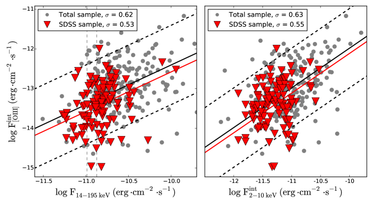
Figure 5: Plots of the [O iii] $\lambda 5007$ extinction corrected flux vs the two X-ray fluxes. The red triangles represent the sources observed by SDSS (110 objects). The black line is a one-to-one fit of the total sample and the red line a one-to-one fit of the SDSS sub-sample. The scatter and the fit of the sub-sample are comparable to the ones of the main sample.

The BASS survey gathered optical spectra from various instruments with different data qualities (i.e., resolution, sensitivity, wavelength range). This lack of homogeneity in the data could artificially increase the scatter in the [O iii]« – »X-ray relation. For this reason, we also analyze the SDSS sub-sample (110 AGN) because of their high quality in flux calibration (Figure 5). We find that the scatter decreases by 0.09 dex for the 14$-$195 keV and 0.08 dex for the 2$-$10 keV band. In order to have a quantitative result for this change in scatter, we run again a Levene’s test. The resulting $p$-values for the SDSS sub-sample are respectively 0.062 and 0.35 for the BAT and 2$-$10 keV X-ray bands which is not statistically significant. The fit of the SDSS sub-sample (red line) is similar to the fit of the total sample (black line) for both X-ray bands. This implies that we do not have any statistical offset due to systematics (like flux calibration issue). We conclude that there is no significant difference between the total sample and the SDSS sub-sample.

4.2 X-ray correlation with high and low ionization lines

Lines produced from high ionization ($>$40 eV) have the advantage of being less contaminated by host galaxy emission than lines produced from low ionization ($<$20 eV). Moreover, these lines are emitted in less extended regions, which implies that we cover a larger portion of their emitting regions in our observations than for low ionization lines. Finally, we include the H$\alpha$ and H$\beta$ emission lines as these lines are either not or less affected with respect to other lines by variations in metal abundances, ionization levels, and collisional effects.

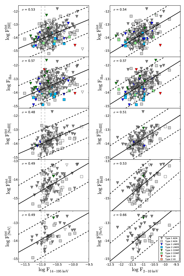
Figure 6: Plots of the relation between five optical narrow emission lines ([S ii]$\,\lambda 6717,6731$, H$\alpha$, He ii $\lambda 4686$, [Ne iii] $\lambda 3869$ and [Ne v] $\lambda 3426$) with the BAT X-ray flux (left) and with the intrinsic 2$-$10 keV flux (right). The plots show subsamples where the particular emission line is detected. The flux units are in $erg\cdot cm^{-2}\cdot s^{-1}$. The subplots are vertically ordered by ionization level of the emission line. The black lines are one-to-one fits of the data. The color code represents the [N ii] BPT classification. White symbols do not have any BPT classification because of undetected emission lines.

Figure 6 illustrates the various emission line fluxes as a function of the two X-ray fluxes. Our data show that the correlation is slightly stronger with [Ne iii], He ii or [Ne v] than with [O iii], H$\alpha$ or [S ii], especially for the BAT X-ray band. Their scatter is smaller by about $\sim$0.09 dex and the correlation coefficient increases from $\rm{R_{Pear}\sim 0.36}$ to $\rm{R_{Pear}\sim 0.44}$. However, the [Ne v] emission line is only detected in optically selected AGNs with very bright emission lines whereas the [O iii] line is detected in many faint AGN such as the LINERs and composite objects which has the effect to increase the scatter. To overcome these possible biases, we need to compare the same samples together. This is what we show in Table 2. In this table, the reported standard deviations and Pearson coefficients are calculated based on a sub-sample of objects having both the detection of the considered line and an [O iii] detection. In order to quantitatively investigate if the flux correlation of X-rays with [S ii], H$\alpha$, [Ne iii], He ii or [Ne v] differ significantly from the one with [O iii], we run a $z$-test based on the two Pearson correlation coefficients (Fisher r-to-z transformation). The $p$-value is also reported in Table 2. The result of this statistical analysis shows that we have $p$-value $>$ 0.5 for all emission lines. The small differences between the linear relations are therefore not statistically significant.

4.3 Relationships between optical emission lines

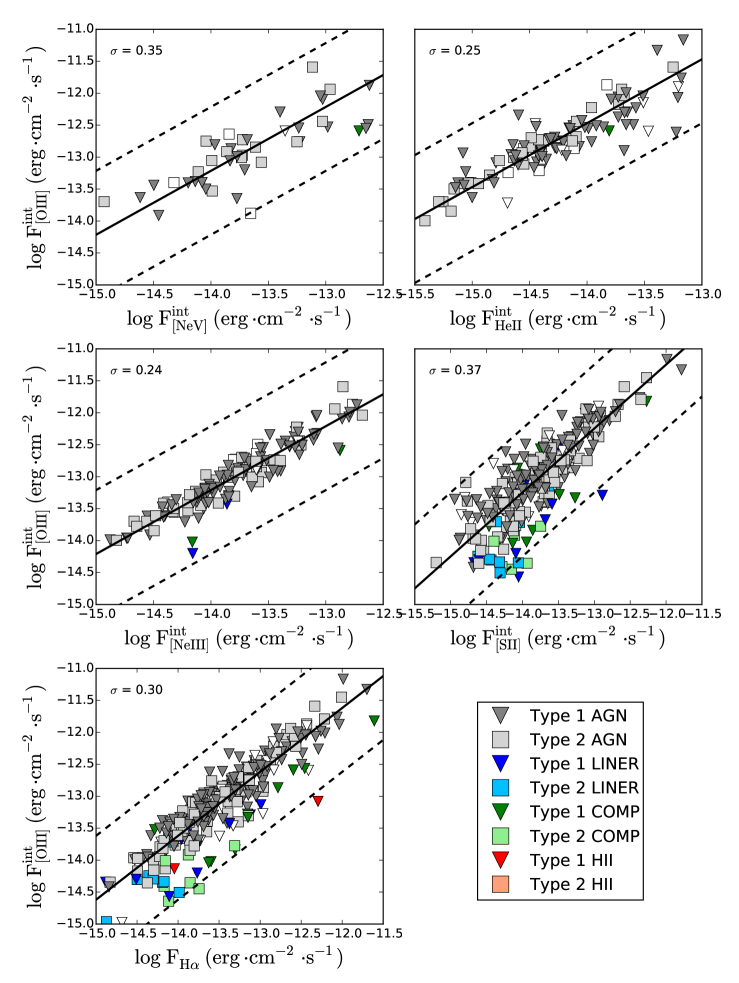
Figure 7: Plots of the relation between optical narrow emission lines and the [O iii] $\lambda 5007$ line in flux space. The plots show subsamples where the particular emission line is detected. The lines are all strongly correlated with [O iii]. The black lines are one-to-one fits of the data. The color code represents the [N ii] BPT classification. White symbols do not have any BPT classification because of undetected emission lines.

Figure 7 shows the relation between [O iii] and other optical emission lines. We see from the scatter ($\sim$0.3 dex) that these emission lines are tightly correlated together. The mean flux ratios, standard deviations and Pearson coefficients are summarized in Table 3. One can especially notice the [O iii]« – »[Ne iii] relation that exhibits a scatter of $\sigma=0.24$ dex. The two transitions originate from ions with comparable ionization energies (35.1 and 41 eV, respectively), and from gas with comparable critical densities ($\mathrm{5\times 10^{5}\ cm^{-3}}$ and $\mathrm{7\times 10^{6}\ cm^{-3}}$, respectively; Kogure & Leung, 2007) which may explain the small scatter.

5 Summary and Discussion

We have presented a study of emission line properties of the largest hard X-ray selected sample of AGN in the local Universe. Our conclusions are:

1. We find very weak correlations with a large scatter (0.62-0.63 dex) between the two X-ray fluxes (2$-$10 keV and 14$-$195 keV band) and the observed and dust corrected [O iii]. The ratios between the X-ray fluxes and the [O iii] corrected flux are $F_{14-195}=(267\pm 22)\times F_{\left[{\rm O}\,\textsc{iii}\right]}^{int}$ and $F_{2-10}=(102\pm 8)\times F_{\left[{\rm O}\,\textsc{iii}\right]}^{int}$.

2. The correlation of emission lines with high ionization levels ([Ne iii], He ii, [Ne v]) with the X-ray flux is not significantly better than for [O iii]. This is also true for the lower ionization line [S ii] and the H$\alpha$ recombination line as compared to [O iii]. While objects which have a [Ne v], He ii or [Ne iii] detection have a smaller scatter ($\sigma^{{\rm Ne}\,\textsc{v}}_{\left[{\rm O}\,\textsc{iii}\right]}=0.49$, $\sigma^{{\rm Ne}\,\textsc{iii}}_{\left[{\rm O}\,\textsc{iii}\right]}=0.47$, $\sigma^{{\rm He}\,\textsc{ii}}_{\left[{\rm O}\,\textsc{iii}\right]}=0.45$), this is only because they have brighter emission lines that exclude the population of LINERS or X-ray detected AGN classified as HII/comp. In general, all lines show a statistically similar level of scatter with the X-rays independent of ionization energy.

3. All the optical emission lines are strongly correlated with [O iii]. These correlations ($\sigma\approx 0.3$) are significantly tighter than what we find between [O iii] and the X-rays.

4. The [O iii]/X-ray flux ratio as a function of the column density ($N_{\rm H}$) is consistent with being constant. However, we see a strong increase in the scatter above $N_{\rm H}$$>10^{22}$ cm^-2 ($\sigma_{<22}=0.47$, $\sigma_{>22}=0.72$). Our results show that the scatter slightly decreases towards larger physical slit sizes in kpc while the ratio $L_{\left[{\rm O}\,\textsc{iii}\right]}^{int}/L_{X}$ is constant for the AGN in our sample ($z>0.01$).

We find that our study agrees well with past studies of X-ray selected AGN, but shows a weaker correlation than [O iii] selected samples which exclude X-ray selected AGN with weak emission lines (e.g., LINERs and optically elusive AGN classified as HII/comp). The correlation we find between the [O iii] corrected luminosity and BAT X-ray luminosity agrees with the 9-month sample of BAT AGN (e.g., $\rm{R_{Pear}^{2}=0.41}$ vs. $\rm{R_{Pear}^{2}\approx}$ 0.35-0.40; Winter et al., 2010). Our correlation result disagrees significantly with the 9-month sample of Meléndez et al. (2008) which compared 2$-$10 keV X-ray fluxes from the ASCA database which are not calculated using detailed X-ray modeling. Panessa et al. (2006) calculated the correlation between the [O iii] corrected flux and the 2$-$10 keV flux from a sample of 47 nearby Seyfert galaxies from the Palomar optical spectroscopic survey (Ho et al., 1995). They obtained a strong Spearman correlation coefficient of $r_{S}=0.78$ that is also not in accordance with this work ($r_{S}=0.39$) most likely because their sample was optically selected and did not include AGN that were X-ray weak. Our results show a slightly higher scatter than the [O iii]« – »X-ray relation in Heckman et al. (2005) ($\sigma=0.51$; this work: $\sigma=0.62$) whose data come from the RXTE slew survey (3-20 keV).

We find no significant evidence of a weakening or strengthening of line emission at high AGN luminosities. This is because of the very weak correlation and large scatter which make a linear model inappropriate (e.g. Hogg et al. 2010). The improvement in the scatter of a linear fit is very small ($\approx$ 0.01 dex) over a simple one-to-one relation between [O iii] and X-ray luminosity. Using the OLS bisector method, the best slope between the intrinsic [O iii] and the 14$-$195 keV luminosity is $1.29\pm 0.05$ and the intrinsic [O iii] and 2$-$10 keV luminosity is $1.23\pm 0.05$. This is in accordance with previous BAT studies (e.g., $1.16\pm 0.20$; Winter et al., 2010). Alternatively, the EM method including censured data finds a slope of $0.83\pm 0.06$ which is consistent with past studies using the same line fitting method as found in Meléndez et al. 2008 ($0.8\pm 0.1$) or Panessa et al. 2006 ($0.82\pm 0.04$). In summary, our best fit slope is consistent with past studies, though the large intrinsic scatter of the relation yields very different results depending on the line fitting method used.

Our analysis shows that the relation between optical emission lines and hard X-rays exist, but is very weak (at best $\sigma\sim$0.5 dex), no matter which optical emission line ([S ii], H$\alpha$, [O iii], [Ne iii], He ii, [Ne v]) or which X-ray flux (2$-$10 keV intrinsic or 14$-$195 keV). Additionally, calibration, obscuration, and physical slit size play only a small role in the scatter. This scatter is much larger than the scatter of X-ray compared to SED fits of unobscured BAT AGN using the UV (e.g., 14$-$195 keV scatter of 0.3 dex, Vasudevan et al., 2009). While our analysis focused on the hard X-rays ($>$2 keV), the soft X-rays ($<$2 keV) have been shown to be dominated by emission lines in several Seyfert AGN whose extended spatial profiles show morphological correlations with the [O iii] (e.g. Bianchi 2006, Wang et al. 2011, Koss et al. 2015). Thus, the soft X-rays coming from the emission line regions may shower a tighter correlation that is worth investigating in future studies.

These results therefore strongly suggest that the majority of the intrinsic scatter has physical origins related to the NLR gas. There are several mechanisms such as covering factor of the narrow-line region gas (e.g., Netzer & Laor, 1993; Noguchi et al., 2010), density dependence of [O iii] (Crenshaw & Kraemer, 2005), differing ionization parameter (Baskin & Laor, 2005), contamination of the narrow emission lines from star formation (e.g., Wild et al., 2011), errors in the Balmer decrement because of different distribution of Balmer lines and forbidden lines, and finally SED shape changes with luminosity (Netzer et al., 2006). Another possibility is AGN variability, where the X-ray emission varies on very short time scales (sub-parsec scale) and represents the instantaneous accretion rate while the NLR which is orders of magnitude larger than the corona (100 parsec to kiloparsec scale), varies on much longer time scales and traces the average accretion rate (e.g., Mushotzky et al., 1993; Schawinski et al., 2015). Future studies using high signal-to-noise Integral Field Unit (IFU) observations with wide wavelength coverage of large samples of AGN such as the Multi Unit Spectroscopic Explorer (MUSE; Bacon et al., 2010) are critical to map and study the importance of these different parameters. Finally, the Nuclear Spectroscopic Telescope Array (NuSTAR; Harrison et al., 2013) hard X-ray telescope is currently observing many BAT AGN as part of the legacy survey (Baloković et al., in prep.) with a 100 times increase in sensitivity which improves estimates of X-ray luminosity compared to BAT.

Table 1: [O iii]« – »X-ray luminosity relations for different sub-samples

Y	X	Sample	N	a	b	$\sigma$	$<$X$>$	$<$Y$>$
(1)	(2)	(3)	(4)	(5)	(6)	(7)	(8)	(9)
		all	327	1.29$\pm$0.05	-15$\pm$2	0.61	43.9	41.4
		Type 1-1.9	215	1.17$\pm$0.06	-9.6$\pm$2.6	0.53	44.0	41.6
		Type 2.0	112	1.40$\pm$0.10	-20$\pm$4	0.69	43.7	41.1
$\log\ L_{\left[{\rm O}\,\textsc{iii}\right]}^{int}$	$\log\ L_{14-195}$
		Seyferts	241	1.16$\pm$0.05	-9.3$\pm$2.4	0.53	43.9	41.5
		LINERs	17	1.8$\pm$0.3	-39$\pm$13	0.70	43.6	40.5
		HII/comp/ambiguous	17	1.2$\pm$0.2	-11$\pm$8	0.74	43.7	40.9
		all	321	1.23$\pm$0.05	-12$\pm$2	0.61	43.5	41.4
		Type 1-1.9	209	1.10$\pm$0.06	-6.5$\pm$2.5	0.56	43.6	41.6
		Type 2.0	112	1.30$\pm$0.10	-15$\pm$4	0.69	43.3	41.1
$\log\ L_{\left[{\rm O}\,\textsc{iii}\right]}^{int}$	$\log\ L_{2-10}^{int}$
		Seyferts	238	1.13$\pm$0.05	-7.5$\pm$2.3	0.54	43.4	41.5
		LINERs	17	1.8$\pm$0.3	-37$\pm$12	0.62	43.1	40.5
		HII/comp/ambiguous	16	1.0$\pm$0.2	-4$\pm$8	0.62	43.2	40.8

Note. « — » (1) variable Y ; (2) variable X ; (3) AGN type : type 1-1.9 are all the objects with broad H$\alpha$ detection, type 2 are all the objects without broad detection, LINERs are selected by the [S ii] and [O i] diagrams, HII/comp/ambiguous and Seyferts are selected by the [N ii] diagram (except for previously selected LINERs); (4) size of sample ; (5) slope with its 1-$\sigma$ uncertainty ; (6) regression intercept with its 1-$\sigma$ uncertainty. The equation of the linear regression is Y = aX + b ; (7) standard deviation ; (8) mean value of X ; (9) mean value of Y.

Table 2: Relations of various optical emission lines intrinsic fluxes with the 14$-$195 keV emission and the comparison with the [O iii]« – »14$-$195 keV relation.

Line	$\chi$ [eV]	N	$\sigma_{\left[{\rm O}\,\textsc{iii}\right]}$	$\sigma_{Line}$	$\rm{R_{Pear,\ \left[{\rm O}\,\textsc{iii}\right]}}$	$\rm{R_{Pear,\ Line}}$	$p$-value
(1)	(2)	(3)	(4)	(5)	(6)	(7)	(8)
[O i]$\,\lambda 6300$	.	206	0.60 dex	0.53 dex	0.41	0.46	0.54
[S ii]$\,\lambda 6717,6731$	10.4	275	0.61 dex	0.53 dex	0.37	0.38	0.89
H$\alpha$	13.6	296	0.62 dex	0.57 dex	0.36	0.34	0.78
[N ii]$\,\lambda 6583$	14.5	277	0.62 dex	0.56 dex	0.37	0.36	0.89
[Ne iii]$\,\lambda 3968$	41.0	144	0.47 dex	0.48 dex	0.45	0.44	0.92
He ii $\lambda 4686$	54.4	106	0.45 dex	0.49 dex	0.49	0.42	0.53
[Ne v]$\,\lambda 3426$	97.1	51	0.49 dex	0.49 dex	0.42	0.45	0.86

Note. « — » (1) optical emission line ; (2) ionization level ; (3) size of the common sample in which both the Line and [O iii] are detected ; (4) standard deviation and (5) Pearson R coefficient of the $\log\ F_{\left[{\rm O}\,\textsc{iii}\right]}^{int}$« – »$\log\ F_{14-195}$ relation ; (6) standard deviation and (7) Pearson R coefficient of the $\log\ F_{Line}^{int}$« – »$\log\ F_{14-195}$ relation ; (8) $p$-value of the null hypothesis that the two correlation coefficients obtained from independent parent samples are equal.

Table 3: Correlation between [O iii] $\lambda 5007$ and other optical emission line intrinsic fluxes.

Line	$\chi$ [eV]	N	$<r>$	$\sigma$	$\rm{R_{Pear}}$
(1)	(2)	(3)	(4)	(5)	(6)
[O i]$\,\lambda 6300$	.	206	0.050	0.36 dex	0.84
[S ii]$\,\lambda 6717,6731$	10.4	275	0.19	0.37 dex	0.83
H$\alpha$	13.6	296	0.438	0.30 dex	0.90
[N ii]$\,\lambda 6583$	14.5	277	0.30	0.40 dex	0.81
[Ne iii]$\,\lambda 3968$	41.0	138	0.17	0.24 dex	0.89
He ii $\lambda 4686$	54.4	106	0.031	0.25 dex	0.88
[Ne v]$\,\lambda 3426$	97.1	43	0.18	0.35 dex	0.79

Note. « — » (1) optical emission line ; (2) ionization level ; (3) size of the sample ; (4) mean flux ratio ; (5) standard deviation ; (6) Pearson R coefficient.

References

- Alam et al. (2015) Alam S., Albareti F. D., Allende Prieto C., Anders F., Anderson S. F., Andrews B. H., Armengaud E., Aubourg É., Bailey S., Bautista J. E., et al. 2015, ArXiv e-prints
- Antonucci (1993) Antonucci R., 1993, ARA&A, 31, 473
- Bacon et al. (2010) Bacon R., Accardo M., Adjali L., Anwand H., Bauer S., Biswas I., Blaizot J., Boudon D., Brau-Nogue S., Brinchmann J., 2010, in Society of Photo-Optical Instrumentation Engineers (SPIE) Conference Series Vol. 7735 of Society of Photo-Optical Instrumentation Engineers (SPIE) Conference Series, The MUSE second-generation VLT instrument. p. 8
- Baldwin et al. (1981) Baldwin J. A., Phillips M. M., Terlevich R., 1981, PASP, 93, 5
- Baskin & Laor (2005) Baskin A., Laor A., 2005, MNRAS, 358, 1043
- Baumgartner et al. (2013) Baumgartner W. H., Tueller J., Markwardt C. B., Skinner G. K., Barthelmy S., Mushotzky R. F., Evans P. A., Gehrels N., 2013, ApJS, 207, 19
- Brightman et al. (2015) Brightman M., Baloković M., Stern D., Arévalo P., Ballantyne D. R., Bauer F. E., Boggs S. E., Craig W. W., Christensen F. E., Comastri A., Fuerst F., 2015, ApJ, 805, 41
- Cappellari & Emsellem (2004) Cappellari M., Emsellem E., 2004, PASP, 116, 138
- Cardelli et al. (1989) Cardelli J. A., Clayton G. C., Mathis J. S., 1989, ApJ, 345, 245
- Crenshaw & Kraemer (2005) Crenshaw D. M., Kraemer S. B., 2005, ApJ, 625, 680
- Ferland & Osterbrock (1986) Ferland G. J., Osterbrock D. E., 1986, ApJ, 300, 658
- Ginsburg & Mirocha (2011) Ginsburg A., Mirocha J., , 2011, PySpecKit: Python Spectroscopic Toolkit, Astrophysics Source Code Library
- Hainline et al. (2013) Hainline K. N., Hickox R., Greene J. E., Myers A. D., Zakamska N. L., 2013, ApJ, 774, 145
- Harrison et al. (2013) Harrison F. A., Craig W. W., Christensen F. E., Hailey C. J., Zhang W. W., Boggs S. E., Stern D., Cook W. R., Forster K., Giommi P., 2013, ApJ, 770, 103
- Heckman et al. (2004) Heckman T. M., Kauffmann G., Brinchmann J., Charlot S., Tremonti C., White S. D. M., 2004, ApJ, 613, 109
- Heckman et al. (2005) Heckman T. M., Ptak A., Hornschemeier A., Kauffmann G., 2005, ApJ, 634, 161
- Ho et al. (1995) Ho L. C., Filippenko A. V., Sargent W. L., 1995, ApJS, 98, 477
- Jones et al. (2009) Jones D. H., Read M. A., Saunders W., Colless M., Jarrett 2009, MNRAS, 399, 683
- Kauffmann & Heckman (2009) Kauffmann G., Heckman T. M., 2009, MNRAS, 397, 135
- Kewley et al. (2006) Kewley L. J., Groves B., Kauffmann G., Heckman T., 2006, MNRAS, 372, 961
- Kogure & Leung (2007) Kogure T., Leung K.-C., eds, 2007, The Astrophysics of Emission-Line Stars. Vol. 342 of Astrophysics and Space Science Library
- LaMassa et al. (2009) LaMassa S. M., Heckman T. M., Ptak A., Hornschemeier A., Martins L., Sonnentrucker P., Tremonti C., 2009, ApJ, 705, 568
- Lamastra et al. (2009) Lamastra A., Bianchi S., Matt G., Perola G. C., Barcons X., Carrera F. J., 2009, A&A, 504, 73
- Lawrence (1991) Lawrence A., 1991, MNRAS, 252, 586
- Massaro et al. (2009) Massaro E., Giommi P., Leto C., Marchegiani P., Maselli A., Perri M., Piranomonte S., Sclavi S., 2009, A&A, 495, 691
- Meléndez et al. (2008) Meléndez M., Kraemer S. B., Armentrout B. K., Deo R. P., Crenshaw D. M., Schmitt H. R., Mushotzky R. F., Tueller J., Markwardt C. B., Winter L., 2008, ApJ, 682, 94
- Mor et al. (2009) Mor R., Netzer H., Elitzur M., 2009, ApJ, 705, 298
- Mushotzky et al. (1993) Mushotzky R. F., Done C., Pounds K. A., 1993, ARA&A, 31, 717
- Netzer (2013) Netzer H., 2013, The Physics and Evolution of Active Galactic Nuclei. Cambridge University Press
- Netzer & Laor (1993) Netzer H., Laor A., 1993, ApJ, 404, L51
- Netzer et al. (2006) Netzer H., Mainieri V., Rosati P., Trakhtenbrot B., 2006, A&A, 453, 525
- Noguchi et al. (2010) Noguchi K., Terashima Y., Ishino Y., Hashimoto Y., Koss M., Ueda Y., Awaki H., 2010, ApJ, 711, 144
- Ofek et al. (2007) Ofek E. O., Oguri M., Jackson N., Inada N., Kayo I., 2007, MNRAS, 382, 412
- Panessa et al. (2006) Panessa F., Bassani L., Cappi M., Dadina M., Barcons X., Carrera F. J., Ho L. C., Iwasawa K., 2006, A&A, 455, 173
- Revnivtsev et al. (2004) Revnivtsev M., Sazonov S., Jahoda K., Gilfanov M., 2004, A&A, 418, 927
- Sazonov & Revnivtsev (2004) Sazonov S. Y., Revnivtsev M. G., 2004, A&A, 423, 469
- Schawinski et al. (2015) Schawinski K., Koss M., Berney S., Sartori L. F., 2015, MNRAS, 451, 2517
- Simpson (1998) Simpson C., 1998, MNRAS, 297, L39
- Simpson (2005) Simpson C., 2005, MNRAS, 360, 565
- Steffen et al. (2006) Steffen A. T., Strateva I., Brandt W. N., Alexander D. M., Koekemoer A. M., Lehmer B. D., Schneider D. P., Vignali C., 2006, AJ, 131, 2826
- Tueller et al. (2008) Tueller J., Mushotzky R. F., Barthelmy S., Cannizzo J. K., Gehrels N., Markwardt C. B., Skinner G. K., Winter L. M., 2008, ApJ, 681, 113
- Ueda et al. (2007) Ueda Y., Eguchi S., Terashima Y., Mushotzky R., Tueller J., Markwardt C., Gehrels N., Hashimoto Y., Potter S., 2007, ApJ, 664, L79
- Urry et al. (1991) Urry C. M., Maraschi L., Phinney E. S., 1991, Comments on Astrophysics, 15, 111
- Urry & Padovani (1995) Urry C. M., Padovani P., 1995, PASP, 107, 803
- Vasudevan et al. (2009) Vasudevan R. V., Mushotzky R. F., Winter L. M., Fabian A. C., 2009, MNRAS, 399, 1553
- Veilleux & Osterbrock (1987) Veilleux S., Osterbrock D. E., 1987, ApJS, 63, 295
- Wild et al. (2011) Wild V., Groves B., Heckman T., Sonnentrucker P., Armus L., Schiminovich D., Johnson B., Martins L., Lamassa S., 2011, MNRAS, 410, 1593
- Winter et al. (2010) Winter L. M., Lewis K. T., Koss M., Veilleux S., Keeney B., Mushotzky R. F., 2010, ApJ, 710, 503
- Young et al. (2010) Young M., Elvis M., Risaliti G., 2010, ApJ, 708, 1388