Integrability of Smooth Wilson Loops
in $\mathcal{N}=4$ Superspace

Niklas Beisert, Dennis Müller, Jan Plefka, Cristian Vergu


HU-EP-15/33

arxiv:1509.05403
Integrability of Smooth Wilson Loops
in $\mathcal{N}=4$ Superspace
Niklas Beisert1, Dennis Müller2, Jan Plefka1,2
and Cristian Vergu1,3
1 Institut für Theoretische Physik,
Eidgenössische Technische Hochschule Zürich,
Wolfgang-Pauli-Strasse 27, 8093 Zürich, Switzerland
nbeisert@itp.phys.ethz.ch
2 Institut für Physik und IRIS Adlershof,
Humboldt-Universität zu Berlin, §
Zum Großen Windkanal 6, D-12489 Berlin, Germany
{dmueller,plefka}@physik.hu-berlin.de 3 Department of Mathematics, King’s College London
The Strand, WC2R 2LS, London, UK
c.vergu@gmail.com Abstract We perform a detailed study of the Yangian symmetry of smooth supersymmetric Maldacena–Wilson loops in planar 𝒩=4𝒩4\mathcal{N}=4 super Yang–Mills theory. This hidden symmetry extends the global superconformal symmetry present for these observables. A gauge-covariant action of the Yangian generators on the Wilson line is established that generalizes previous constructions built upon path variations. Employing these generators the Yangian symmetry is proven for general paths in non-chiral 𝒩=4𝒩4\mathcal{N}=4 superspace at the first perturbative order. The bi-local piece of the level-one generators requires the use of a regulator due to divergences in the coincidence limit. We perform regularization by point splitting in detail, thereby constructing additional local and boundary contributions as regularization for all level-one Yangian generators. Moreover, the Yangian algebra at level one is checked and compatibility with local kappa-symmetry is established. Finally, the consistency of the Yangian symmetry is shown to depend on two properties: The vanishing of the dual Coxeter number of the underlying superconformal algebra and the existence of a novel superspace “G-identity” for the gauge field theory. This tightly constrains the conformal gauge theories to which integrability can possibly apply.
   

1 Introduction

The maximally supersymmetric gauge field theory in four dimensions [1, 2]𝒩=4𝒩4\mathcal{N}=4 super Yang–Mills (SYM) – with SU(N)SU𝑁\mathrm{SU}(N) gauge group has become something like the drosophila of gauge field theories. This is due to its remarkable symmetry structure and the observed integrability [3] in the planar limit of the theory. Integrability arises in particular in the spectral problem of scaling dimensions of local gauge-invariant operators [4, 5] and (tree-level) scattering amplitudes [6]. Wilson loop operators [7] constitute another prominent class of gauge-invariant observables for quantum gauge field theories. In ordinary gauge theories, they serve as order parameters for confinement. For conformal and thus non-confining 𝒩=4𝒩4\mathcal{N}=4 SYM, they are of relevance because they may, in principle, provide an ideal testing ground for integrability. According to the AdS/CFT correspondence [8] the 𝒩=4𝒩4\mathcal{N}=4 SYM model is dual to the type IIB superstring on an AdS5×S5𝐴𝑑subscript𝑆5superscript𝑆5AdS_{5}\times S^{5} space-time background. Within this setting there is a natural Wilson loop for 𝒩=4𝒩4\mathcal{N}=4 SYM that extends the standard definition, where one integrates the gauge field Aμsubscript𝐴𝜇A_{\mu} along a closed path in 1,3superscript13\mathbb{R}^{1,3}. The presence of six real adjoint scalar fields in the theory allows for a coupling to an extended path C~~𝐶\tilde{C} on 1,3×S5superscript13superscript𝑆5\mathbb{R}^{1,3}\times S^{5}, to wit [9, 10]

1NtrW=1NtrPexp(C~dτ(x˙μAμ(x)+nix˙μx˙μϕi(x)))with (ni)2=1.formulae-sequence1𝑁tr𝑊1𝑁trPsubscriptcontour-integral~𝐶differential-d𝜏superscript˙𝑥𝜇subscript𝐴𝜇𝑥superscript𝑛𝑖superscript˙𝑥𝜇subscript˙𝑥𝜇subscriptitalic-ϕ𝑖𝑥with superscriptsuperscript𝑛𝑖21\frac{1}{N}\operatorname{tr}W=\frac{1}{N}\operatorname{tr}\operatorname{P}\exp{\left(\oint_{\tilde{C}}\mathrm{d}\tau\left(\dot{x}^{\mu}A_{\mu}(x)+n^{i}\sqrt{\dot{x}^{\mu}\dot{x}_{\mu}}\,\phi_{i}(x)\right)\right)}\qquad\text{with }~{}(n^{i})^{2}=1\,. (1.1)

From a ten-dimensional perspective the coupling to the loop C~~𝐶\tilde{C} is such that the path is light-like: x˙2(ni)2x˙2=0superscript˙𝑥2superscriptsuperscript𝑛𝑖2superscript˙𝑥20\dot{x}^{2}-(n^{i})^{2}\,\dot{x}^{2}=0 (using mostly minus signature). This so-called Maldacena–Wilson loop operator is UV-finite and invariant under conformal transformations. Its dual description at strong coupling is given by a minimal (bosonic) string surface in AdS5×S5𝐴𝑑subscript𝑆5superscript𝑆5AdS_{5}\times S^{5} space ending on the boundary at the curve C~~𝐶\tilde{C}.

However, it is clear that the operator W𝑊W is merely the leading component of a supersymmetric object generalizing the path C~~𝐶\tilde{C} into superspace. This is necessary in order to have a Wilson loop which respects the ordinary \mathbb{Q} and conformal 𝕊𝕊\mathbb{S} supersymmetries of 𝒩=4𝒩4\mathcal{N}=4 SYM. Such a super Maldacena–Wilson loop was first considered in [11] and further studied in [12]. The complete definition and a detailed study of its local symmetries was recently performed by us [13]. It is defined as

1Ntr𝒲=1NtrPexp(Z~dτ(\displaystyle\frac{1}{N}\operatorname{tr}{\mathcal{W}}=\frac{1}{N}\operatorname{tr}\operatorname{P}\exp\biggl{(}\oint_{\tilde{Z}}\mathrm{d}\tau\,\Bigr{(} pμ𝒜μcov(x,θ,θ¯)+qiΦi(x,θ,θ¯)superscript𝑝𝜇subscriptsuperscript𝒜cov𝜇𝑥𝜃¯𝜃superscript𝑞𝑖subscriptΦ𝑖𝑥𝜃¯𝜃\displaystyle p^{\mu}\mathcal{A}^{\text{cov}}_{\mu}(x,\theta,\bar{\theta})+q^{i}\,\Phi_{i}(x,\theta,\bar{\theta})\,
+θ˙aα𝒜αacov(x,θ,θ¯)+θ¯˙α˙𝒜covaa(x,θ,θ¯)α˙)),\displaystyle+\dot{\theta}^{a\alpha}\mathcal{A}^{\text{cov}}_{\alpha a}(x,\theta,\bar{\theta})+\dot{\bar{\theta}}^{\dot{\alpha}}{}_{a}\,\mathcal{A}^{\text{cov}\,a}{}_{\dot{\alpha}}(x,\theta,\bar{\theta})\Bigr{)}\,\biggr{)}\,, (1.2)

where Z~={x,θ,θ¯;q}~𝑍𝑥𝜃¯𝜃𝑞\tilde{Z}=\{x,\theta,\bar{\theta};q\} defines a path in a non-chiral 𝒩=4𝒩4\mathcal{N}=4 superspace extended by coordinates qisuperscript𝑞𝑖q^{i} on an auxiliary space 6superscript6\mathbb{R}^{6}. The combination pμ=x˙μ+θσμθ¯˙θ˙σμθ¯superscript𝑝𝜇superscript˙𝑥𝜇𝜃superscript𝜎𝜇˙¯𝜃˙𝜃superscript𝜎𝜇¯𝜃p^{\mu}=\dot{x}^{\mu}+\theta\sigma^{\mu}\dot{\bar{\theta}}-\dot{\theta}\sigma^{\mu}\bar{\theta} is a covariant generalization of x˙μsuperscript˙𝑥𝜇\dot{x}^{\mu}, and the constraint qiqi=pμpμsuperscript𝑞𝑖superscript𝑞𝑖superscript𝑝𝜇subscript𝑝𝜇q^{i}q^{i}=p^{\mu}p_{\mu} restricts the path on the internal space to a sphere S56superscript𝑆5superscript6S^{5}\subset\mathbb{R}^{6} in analogy to (ni)2=1superscriptsuperscript𝑛𝑖21(n^{i})^{2}=1. Furthermore, 𝒜μcovsubscriptsuperscript𝒜cov𝜇\mathcal{A}^{\text{cov}}_{\mu}, 𝒜αacovsubscriptsuperscript𝒜cov𝛼𝑎\mathcal{A}^{\text{cov}}_{\alpha a}, 𝒜covaα˙\mathcal{A}^{\text{cov}\,a}{}_{\dot{\alpha}} and ΦisubscriptΦ𝑖\Phi_{i} are fields on superspace.111Note that in our previous work [13] we did not use the superscript “cov” for the connection superfield. Here we do so in order to distinguish from a torsion-free situation. Similarly, 𝒟covsuperscript𝒟cov\mathcal{D}^{\text{cov}} here corresponds to 𝒟𝒟\mathcal{D} in [13]. This Wilson loop operator enjoys superconformal 𝔭𝔰𝔲(2,2|4)𝔭𝔰𝔲2conditional24\mathfrak{psu}(2,2|4) and local kappa-symmetry along the path [13], the latter being a generalization of the local 1/2121/2 BPS property of the bosonic operator (1.1). The expectation value of this operator for closed non-self intersecting smooth paths Z~~𝑍\tilde{Z} is UV-finite at least at the leading non-trivial order in perturbation theory. 222In principle our analysis may be extended to more general UV-divergent cases, see the conclusions for a brief discussion of this.

In [12] the integrability of the above super Maldacena–Wilson loop operator at leading order in the Graßmann coordinates θ𝜃\theta and θ¯¯𝜃\bar{\theta} was demonstrated: The one-loop vacuum expectation value \bBigg@0tr𝒲\bBigg@0\mathopen{\bBigg@{0}}\langle\operatorname{tr}\mathcal{W}\mathclose{\bBigg@{0}}\rangle is invariant under an infinite-dimensional Yangian algebra Y[𝔭𝔰𝔲(2,2|4)]𝑌delimited-[]𝔭𝔰𝔲2conditional24Y[\mathfrak{psu}(2,2|4)] represented by variational operators acting on the path Z~~𝑍\tilde{Z}. In two-dimensional quantum field theory a Yangian symmetry is an expression of integrability, i.e. its Casimir operators imply the existence of an infinite number of conserved local charges which constrain the dynamics substantially.

Recently, the question of Yangian symmetry of the super Maldacena–Wilson loop has been investigated also at strong coupling. Already in the initial paper [12] the level-one Yangian symmetry of the bosonic string minimal surface problem was shown. This was generalized to the full Green–Schwarz superstring minimal surface problem in [14], where the full Y[𝔭𝔰𝔲(2,2|4)]𝑌delimited-[]𝔭𝔰𝔲2conditional24Y[\mathfrak{psu}(2,2|4)] Yangian symmetry could be established and the general solution to the equations of motion ending on the boundary path Z~~𝑍\tilde{Z} was found in the vicinity of the boundary. In [15] the extension of this algebra to the level-one hypercharge bonus Yangian symmetry was determined, mirroring the structure observed for scattering amplitudes [16].

In this work we complete the analysis of smooth super Wilson loops initiated in [13] and address the Yangian invariance of the super Maldacena–Wilson loop (1). In fact there have been previous integrability studies of bosonic Wilson loops in refs. [17, 18, 19, 20, 21, 22]. However, these references studied only contours which were piecewise light-like, x˙2=0superscript˙𝑥20\dot{x}^{2}=0, for which the coupling to the scalars in (1.1) disappears. These light-like polygonal-shaped Wilson loops are dual to maximally-helicity-violating scattering amplitudes in 𝒩=4𝒩4\mathcal{N}=4 SYM [23, 24, 25]. In order to achieve superconformal symmetry for light-like polygonal Wilson loops and to provide a dual to next-to-maximally helicity violating scattering amplitudes, supersymmetric Wilson loops have been considered in chiral [26, 27] and in full non-chiral [28, 29] 𝒩=4𝒩4\mathcal{N}=4 superspace.

However, such Wilson loops suffer from UV-divergences arising through the light-like polygonal contours and their cusps [30]. They parallel the IR-divergences of the massless scattering amplitudes. The standard and very convenient procedure to deal with these divergences is dimensional reduction. Other regularization schemes one may choose for Wilson loops are framing and boxing. The first prevents the divergences by forcing the propagators to end on different contours, while the second defines a finite ratio of Wilson loops [17]. Further regularizations for scattering amplitudes are mass regularization, proposed in ref. [31] and spectral regularization proposed in ref. [32], but they do not appear to have a simple correspondent for Wilson loops. Unfortunately, so far no regulator is known that preserves all the superconformal and Yangian symmetries of the tree-level amplitudes. In contrast, for the smooth non-null Wilson loops of (1) discussed in [11, 12, 13], we expect the superconformal and non-local Yangian symmetry to be non-anomalous as the correlator is finite for smooth paths. We therefore consider them highly natural observables to study within the context of AdS/CFT integrability.

Our paper is organized as follows. In section 2 the action of the superconformal and level-one Yangian generators on the Wilson line operator is constructed. The level-one generators contain a local and a bi-local piece, where the latter is given by the path-ordered product of two level-zero generators. It is shown that gauge covariance necessitates the departure from a variational derivative representation of the level-zero generators acting on the coordinates of the path to a gauge-covariant representation which acts on the fields and is importantly augmented by a compensating gauge transformation. Moreover, we show that the cyclicity of the Wilson loop is compatible with the level-one Yangian generators provided that the dual Coxeter number of the level-zero algebra vanishes (which it does for 𝔭𝔰𝔲(2,2|4)𝔭𝔰𝔲2conditional24\mathfrak{psu}(2,2|4)) and a novel so-called G-identity holds for a particular contraction of the field strength two-form with the conformal Killing vectors. In section 3 the level-one Yangian algebra for our gauge-covariant generators is established and the compatibility with kappa-symmetry is proven. In section 4 we start out with a brief review of the superspace formalism and the results for the two-point functions of our previous work [13]. Then the representation of the superconformal algebra in our 𝒩=4𝒩4\mathcal{N}=4 non-chiral extended superspace {x,θ,θ¯;q}𝑥𝜃¯𝜃𝑞\{x,\theta,\bar{\theta};q\} is given and the above mentioned G-identity is proven. We show in section 5 the Yangian invariance of the vacuum expectation value of an arbitrary smooth super Wilson loop at first perturbative order to all orders in anti-commuting variables. In order to do so it is mandatory to regulate the bi-local part via point splitting in the coincidence limit. This procedure induces the form of the local part of the level-one generators which we construct for all algebra elements. Finally, in section 6 we conclude.

2 Yangian Action on Wilson Lines

In the following we discuss the action of Yangian generators on Wilson line operators in the classical theory. We will take a generic gauge theory rather than 𝒩=4𝒩4\mathcal{N}=4 super Yang–Mills as the starting point for two reasons: On the one hand, it will streamline the discussion, and let us focus on the features of the Yangian algebra. On the other hand, it allows us to see more clearly which of the many exceptional features of 𝒩=4𝒩4\mathcal{N}=4 super Yang–Mills theory are responsible for its integrability.

The Wilson line is defined by

𝒲=Pexpγ𝒜,d𝒲=𝒲𝒜(1)𝒜(0)𝒲,formulae-sequence𝒲Psubscript𝛾𝒜d𝒲𝒲𝒜1𝒜0𝒲\mathcal{W}=\operatorname{P}\exp\int_{\gamma}\mathcal{A},\qquad\mathrm{d}\mathcal{W}=\mathcal{W}\mathcal{A}(1)-\mathcal{A}(0)\mathcal{W}, (2.1)

where γ:τX(τ):𝛾maps-to𝜏𝑋𝜏\gamma:\tau\mapsto X(\tau) is an (open) path between τ=0𝜏0\tau=0 and τ=1𝜏1\tau=1 (for concreteness) and 𝒜𝒜\mathcal{A} is the gauge connection one-form (pulled back to the path). We consider a general spacetime with coordinates X𝒜superscript𝑋𝒜X^{{\mathcal{A}}} on which a conformal algebra can act. The gauge connection can be expanded as 𝒜=dX𝒜𝒜𝒜𝒜dsuperscript𝑋𝒜subscript𝒜𝒜\mathcal{A}=\mathrm{d}X^{\mathcal{A}}\mathcal{A}_{\mathcal{A}} in terms of the flat vielbein dX𝒜dsuperscript𝑋𝒜\mathrm{d}X^{\mathcal{A}}. For the sake of simplicity we shall assume the coordinates to be bosonic throughout this chapter in order to avoid a proliferation of sign factors. The latter can be reinstated for a graded spacetime according to simple rules, see sec. 4.

2.1 Conformal Action on the Wilson Line

We start by defining the action of the conformal generators, which constitute the zeroth level of the Yangian algebra, on the Wilson line. In fact, there are several options for their definition which, ultimately, differ in boundary contributions. Unfortunately, such boundary terms easily spoil Yangian symmetry, by a finite or even an infinite amount. Therefore, a precise definition of the action of the conformal and Yangian generators is crucial.

Action on the path.

A finite element G𝐺G of the conformal group acts on the Wilson loop by transforming the path

G𝒲γ=𝒲Gγ.𝐺subscript𝒲𝛾subscript𝒲𝐺𝛾G\mathcal{W}_{\gamma}=\mathcal{W}_{G\gamma}. (2.2)

For the conformal algebra we consider an infinitesimal group element G=1+ϵJ+𝒪\bBigg@0(ϵ2\bBigg@0)G=1+\epsilon\mathrm{J}+\mathcal{O}\mathopen{\bBigg@{0}}(\epsilon^{2}\mathclose{\bBigg@{0}}) with an algebra generator JJ\mathrm{J} and the expansion parameter ϵitalic-ϵ\epsilon. Supposing that the generator JJ\mathrm{J} acts on the path X(τ)𝑋𝜏X(\tau) by the variational operator 𝐉𝐉\mathbf{J} we can write the action as

𝐉=dτ𝐉(τ),𝐉(τ)=JX𝒜(X(τ))δδX𝒜(τ).formulae-sequence𝐉differential-d𝜏𝐉𝜏𝐉𝜏Jsuperscript𝑋𝒜𝑋𝜏𝛿𝛿superscript𝑋𝒜𝜏\mathbf{J}=\int\mathrm{d}\tau\,\mathbf{J}(\tau),\qquad\mathbf{J}(\tau)=\mathrm{J}X^{{\mathcal{A}}}(X(\tau))\,\frac{\delta}{\delta X^{{\mathcal{A}}}(\tau)}\,. (2.3)

With abuse of notation, JX𝒜(X)Jsuperscript𝑋𝒜𝑋\mathrm{J}X^{{\mathcal{A}}}(X) denotes the infinitesimal conformal displacement of the point X𝒜superscript𝑋𝒜X^{{\mathcal{A}}}. In the conformal action 𝐉(τ)𝐉𝜏\mathbf{J}(\tau) the latter is evaluated on the path X(τ)𝑋𝜏X(\tau). This definition and an analogous one for the Yangian algebra was used in [12] to discuss Yangian invariance of smooth Wilson loops.

Next we act with this generator on a Wilson line. The generator 𝐉(τ)𝐉𝜏\mathbf{J}(\tau) acts on the gauge connection 𝒜(σ)𝒜𝜎\mathcal{A}(\sigma) via the path element dX𝒜=dσσX𝒜dsuperscript𝑋𝒜d𝜎subscript𝜎superscript𝑋𝒜\mathrm{d}X^{\mathcal{A}}=\mathrm{d}\sigma\,\partial_{\sigma}X^{\mathcal{A}} as well as the evaluation point X𝑋X of the gauge field 𝒜𝒜(X)subscript𝒜𝒜𝑋\mathcal{A}_{\mathcal{A}}(X)

𝐉(τ)𝒜(σ)=dσJX𝒜(τ)(𝒜𝒜(σ)σδ(τσ)+σX(σ)𝒜𝒜(σ)δ(τσ)).𝐉𝜏𝒜𝜎d𝜎Jsuperscript𝑋𝒜𝜏subscript𝒜𝒜𝜎subscript𝜎𝛿𝜏𝜎subscript𝜎superscript𝑋𝜎subscript𝒜subscript𝒜𝜎𝛿𝜏𝜎\mathbf{J}(\tau)\mathcal{A}(\sigma)=\mathrm{d}\sigma\,\mathrm{J}X^{{\mathcal{A}}}(\tau)\left(\mathcal{A}_{{\mathcal{A}}}(\sigma)\partial_{\sigma}\delta(\tau-\sigma)+\partial_{\sigma}X^{{\mathcal{B}}}(\sigma)\partial_{{\mathcal{A}}}\mathcal{A}_{{\mathcal{B}}}(\sigma)\delta(\tau-\sigma)\right). (2.4)

It yields the derivative of a delta-function which should be integrated by parts. This leads to boundary terms which will turn out to be troublesome, in particular for the Yangian action. To understand this problem better, let us consider the integral of such a term over the bounded domains σ<σ<σ+subscript𝜎𝜎subscript𝜎\sigma_{-}<\sigma<\sigma_{+} and τ<τ<τ+subscript𝜏𝜏subscript𝜏\tau_{-}<\tau<\tau_{+}

I:=dτdσ[θ(ττ)θ(ττ+)][θ(σσ)θ(σσ+)]σδ(τσ)f(τ,σ).assign𝐼differential-d𝜏differential-d𝜎delimited-[]𝜃𝜏subscript𝜏𝜃𝜏subscript𝜏delimited-[]𝜃𝜎subscript𝜎𝜃𝜎subscript𝜎subscript𝜎𝛿𝜏𝜎𝑓𝜏𝜎I:=\int\mathrm{d}\tau\,\mathrm{d}\sigma\bigl{[}\theta(\tau-\tau_{-})-\theta(\tau-\tau_{+})\bigr{]}\bigl{[}\theta(\sigma-\sigma_{-})-\theta(\sigma-\sigma_{+})\bigr{]}\partial_{\sigma}\delta(\tau-\sigma)\,f(\tau,\sigma). (2.5)

Here we have implemented the boundaries of the integration domains by means of the unit step function θ(τ)𝜃𝜏\theta(\tau). Integration by parts yields I=I1+I2𝐼subscript𝐼1subscript𝐼2I=I_{1}+I_{2} with

I1subscript𝐼1\displaystyle I_{1} =dτdσ[θ(ττ)θ(ττ+)][θ(σσ)θ(σσ+)]δ(τσ)σf(τ,σ)absentdifferential-d𝜏differential-d𝜎delimited-[]𝜃𝜏subscript𝜏𝜃𝜏subscript𝜏delimited-[]𝜃𝜎subscript𝜎𝜃𝜎subscript𝜎𝛿𝜏𝜎subscript𝜎𝑓𝜏𝜎\displaystyle=-\int\mathrm{d}\tau\,\mathrm{d}\sigma\bigl{[}\theta(\tau-\tau_{-})-\theta(\tau-\tau_{+})\bigr{]}\bigl{[}\theta(\sigma-\sigma_{-})-\theta(\sigma-\sigma_{+})\bigr{]}\delta(\tau-\sigma)\,\partial_{\sigma}f(\tau,\sigma)
=dσ[θ(στ)θ(στ+)][θ(σσ)θ(σσ+)](σf)(σ,σ),absentdifferential-d𝜎delimited-[]𝜃𝜎subscript𝜏𝜃𝜎subscript𝜏delimited-[]𝜃𝜎subscript𝜎𝜃𝜎subscript𝜎subscript𝜎𝑓𝜎𝜎\displaystyle=-\int\mathrm{d}\sigma\bigl{[}\theta(\sigma-\tau_{-})-\theta(\sigma-\tau_{+})\bigr{]}\bigl{[}\theta(\sigma-\sigma_{-})-\theta(\sigma-\sigma_{+})\bigr{]}(\partial_{\sigma}f)(\sigma,\sigma), (2.6)
I2subscript𝐼2\displaystyle I_{2} =dτdσ[θ(ττ)θ(ττ+)][δ(σσ)δ(σσ+)]δ(τσ)f(τ,σ)absentdifferential-d𝜏differential-d𝜎delimited-[]𝜃𝜏subscript𝜏𝜃𝜏subscript𝜏delimited-[]𝛿𝜎subscript𝜎𝛿𝜎subscript𝜎𝛿𝜏𝜎𝑓𝜏𝜎\displaystyle=-\int\mathrm{d}\tau\,\mathrm{d}\sigma\bigl{[}\theta(\tau-\tau_{-})-\theta(\tau-\tau_{+})\bigr{]}\bigl{[}\delta(\sigma-\sigma_{-})-\delta(\sigma-\sigma_{+})\bigr{]}\delta(\tau-\sigma)\,f(\tau,\sigma)
$\displaystyle=-\int\mathrm{d}\tau\,\bigl{[}\theta(\tau-\tau_{-})-\theta(\tau-\tau_{+})\bigr{]}\bigl{[}\delta(\tau-\sigma_{-})-\delta(\tau-\sigma_{+})\bigr{]}f(\tau,\tau)$
$\displaystyle=-\bigl{[}\theta(\sigma_{-}-\tau_{-})-\theta(\sigma_{-}-\tau_{+})\bigr{]}f(\sigma_{-},\sigma_{-})+\bigl{[}\theta(\sigma_{+}-\tau_{-})-\theta(\sigma_{+}-\tau_{+})\bigr{]}f(\sigma_{+},\sigma_{+})$
=θ(στ)f(σ,σ)+θ(τ+σ+)f(σ+,σ+).absent𝜃subscript𝜎subscript𝜏𝑓subscript𝜎subscript𝜎𝜃subscript𝜏subscript𝜎𝑓subscript𝜎subscript𝜎\displaystyle=-\theta(\sigma_{-}-\tau_{-})f(\sigma_{-},\sigma_{-})+\theta(\tau_{+}-\sigma_{+})f(\sigma_{+},\sigma_{+}). (2.7)

In the last line we have assumed that σ,τ<σ+,τ+formulae-sequencesubscript𝜎subscript𝜏subscript𝜎subscript𝜏\sigma_{-},\tau_{-}<\sigma_{+},\tau_{+}. The final result implies that the above action 𝐉𝒲𝐉𝒲\mathbf{J}\mathcal{W} on the Wilson line is ambiguous because, naively, the integration domains for 𝐉(τ)𝐉𝜏\mathbf{J}(\tau) and 𝒜(σ)𝒜𝜎\mathcal{A}(\sigma) should coincide. Equating σ±=τ±subscript𝜎plus-or-minussubscript𝜏plus-or-minus\sigma_{\pm}=\tau_{\pm} leads to the ill-defined value θ(0)𝜃0\theta(0) at both integration boundaries. While this problem might be avoidable for conformal transformations of closed Wilson loops, it unfortunately does affect the Yangian action. In fact, these problems are reminiscent of or even related to the ambiguities in defining the Yangian algebra in a relativistic non-linear sigma model identified in [33].

In our case, one might be able to resolve the ambiguity, and thus cure the above problems by specifying more precisely how to treat the endpoints. Nevertheless, we will refrain from using this framework and instead use operator insertions to represent conformal and Yangian transformations.

Action by insertion.

An alternative form of the conformal action on a Wilson line is by operator insertions

𝕁𝒲=dτ𝒲[0,τ](𝕁𝒜)(τ)𝒲[τ,1]=𝒲[𝕁𝒜].𝕁𝒲differential-d𝜏subscript𝒲0𝜏𝕁𝒜𝜏subscript𝒲𝜏1𝒲delimited-[]𝕁𝒜\mathbb{J}\mathcal{W}=\int\mathrm{d}\tau\,\mathcal{W}_{[0,\tau]}\,(\mathbb{J}\mathcal{A})(\tau)\,\mathcal{W}_{[\tau,1]}=\mathcal{W}[\mathbb{J}\mathcal{A}]. (2.8)

Here, 𝕁𝒜𝕁𝒜\mathbb{J}\mathcal{A} is the action of the global conformal generator JJ\mathrm{J} on the one-form field 𝒜𝒜\mathcal{A}, see below. The conformal variation 𝕁𝒲𝕁𝒲\mathbb{J}\mathcal{W} of a Wilson line 𝒲𝒲\mathcal{W} is thus a Wilson line 𝒲[Q]𝒲delimited-[]𝑄\mathcal{W}[Q] with one insertion of the one-form local operator Q(τ)=𝕁𝒜(X(τ))𝑄𝜏𝕁𝒜𝑋𝜏Q(\tau)=\mathbb{J}\mathcal{A}(X(\tau))

𝒲[Q]:=𝒲[0,τ]Q(τ)𝒲[τ,1].assign𝒲delimited-[]𝑄subscript𝒲0𝜏𝑄𝜏subscript𝒲𝜏1\mathcal{W}[Q]:=\int\mathcal{W}_{[0,\tau]}\,Q(\tau)\,\mathcal{W}_{[\tau,1]}. (2.9)

The operator 𝕁𝕁\mathbb{J} acts on the field 𝒜𝒜subscript𝒜𝒜\mathcal{A}_{\mathcal{A}} in analogy to the action on the path in (2.3)

𝕁=ddX(JX𝒜𝒜𝒜(JX)𝒜)δδ𝒜𝒜(X).𝕁superscriptd𝑑𝑋Jsuperscript𝑋subscriptsubscript𝒜𝒜subscript𝒜Jsuperscript𝑋subscript𝒜𝛿𝛿subscript𝒜𝒜𝑋\mathbb{J}=\int\mathrm{d}^{d}X\,\bigl{(}-\mathrm{J}X^{{\mathcal{B}}}\,\partial_{\mathcal{B}}\mathcal{A}_{\mathcal{A}}-\partial_{\mathcal{A}}(\mathrm{J}X^{\mathcal{B}})\,\mathcal{A}_{\mathcal{B}}\bigr{)}\frac{\delta}{\delta\mathcal{A}_{\mathcal{A}}(X)}\,. (2.10)

Effectively, it acts by transforming the argument $X^{\mathcal{B}}$ as well as the index A

𝕁𝒜𝒜=JX𝒜𝒜𝒜(JX)𝒜.𝕁subscript𝒜𝒜Jsuperscript𝑋subscriptsubscript𝒜𝒜subscript𝒜Jsuperscript𝑋subscript𝒜\mathbb{J}\mathcal{A}_{\mathcal{A}}=-\mathrm{J}X^{{\mathcal{B}}}\,\partial_{\mathcal{B}}\mathcal{A}_{\mathcal{A}}-\partial_{\mathcal{A}}(\mathrm{J}X^{\mathcal{B}})\,\mathcal{A}_{\mathcal{B}}. (2.11)

Its action 𝕁𝒜𝕁𝒜\mathbb{J}\mathcal{A} equals minus333The minus sign in the definition is required to match the Lie algebra of field operators 𝕁𝕁\mathbb{J} (which act on the field variables) with the algebra of derivative operators JJ\mathrm{J} (which act on coordinates). Note that this difference effectively flips the order or operators: 𝕁1𝕁2Ψ=𝕁1J2Ψ=J2𝕁1Ψ=J2J1Ψsubscript𝕁1subscript𝕁2Ψsubscript𝕁1subscriptJ2ΨsubscriptJ2subscript𝕁1ΨsubscriptJ2subscriptJ1Ψ\mathbb{J}_{1}\mathbb{J}_{2}\Psi=-\mathbb{J}_{1}\mathrm{J}_{2}\Psi=-\mathrm{J}_{2}\mathbb{J}_{1}\Psi=\mathrm{J}_{2}\mathrm{J}_{1}\Psi. the action of the derivative operator (conformal Killing vector) J=JX𝒜𝒜JJsuperscript𝑋𝒜subscript𝒜\mathrm{J}=\mathrm{J}X^{\mathcal{A}}\partial_{\mathcal{A}} on the one-form field 𝒜𝒜\mathcal{A} (by means of the Lie derivative)

𝕁𝒜𝕁𝒜\displaystyle\mathbb{J}\mathcal{A} =dX𝒜J𝒜𝒜J(dX)𝒜absentdsuperscript𝑋𝒜Jsubscript𝒜𝒜Jdsuperscript𝑋subscript𝒜\displaystyle=-\mathrm{d}X^{\mathcal{A}}\,\mathrm{J}\mathcal{A}_{\mathcal{A}}-\mathrm{J}(\mathrm{d}X^{\mathcal{B}})\,\mathcal{A}_{\mathcal{B}}
=dX𝒜JX𝒜𝒜d(JX)𝒜.absentdsuperscript𝑋𝒜Jsuperscript𝑋subscriptsubscript𝒜𝒜dJsuperscript𝑋subscript𝒜\displaystyle=-\mathrm{d}X^{\mathcal{A}}\,\mathrm{J}X^{{\mathcal{B}}}\,\partial_{\mathcal{B}}\mathcal{A}_{\mathcal{A}}-\mathrm{d}(\mathrm{J}X^{\mathcal{B}})\,\mathcal{A}_{\mathcal{B}}. (2.12)

The conformal algebra is expressed in terms of the structure constants \bBigg@0[Jδ,Jρ\bBigg@0]=fδρJκκ\mathopen{\bBigg@{0}}[\mathrm{J}^{\delta},\mathrm{J}^{{\rho}}\mathclose{\bBigg@{0}}]=f^{{\delta}{\rho}}{}_{{\kappa}}\mathrm{J}^{{\kappa}}. By construction the conformal action on the field satisfies the same algebra

\bBigg@0[𝕁δ,𝕁ρ\bBigg@0]=fδρ𝕁κκ.\mathopen{\bBigg@{0}}[\mathbb{J}^{\delta},\mathbb{J}^{{\rho}}\mathclose{\bBigg@{0}}]=f^{{\delta}{\rho}}{}_{{\kappa}}\mathbb{J}^{{\kappa}}. (2.13)

Comparison.

Let us compare the two above definitions of the conformal action. To compute the action on the former, we continue at (2.4), use translation invariance of the delta-function, σδ(τσ)=τδ(τσ)subscript𝜎𝛿𝜏𝜎subscript𝜏𝛿𝜏𝜎\partial_{\sigma}\delta(\tau-\sigma)=-\partial_{\tau}\delta(\tau-\sigma), and subsequently perform integration by parts on τ𝜏\tau

𝐉𝒲𝐉𝒲\displaystyle\mathbf{J}\mathcal{W} =dτdσJX𝒜(τ)𝒲[0,σ](𝒜𝒜(σ)σδ(τσ)+σX(σ)𝒜𝒜(σ)δ(τσ))𝒲[σ,1]absentdifferential-d𝜏differential-d𝜎Jsuperscript𝑋𝒜𝜏subscript𝒲0𝜎subscript𝒜𝒜𝜎subscript𝜎𝛿𝜏𝜎subscript𝜎superscript𝑋𝜎subscript𝒜subscript𝒜𝜎𝛿𝜏𝜎subscript𝒲𝜎1\displaystyle=\int\mathrm{d}\tau\,\mathrm{d}\sigma\,\mathrm{J}X^{{\mathcal{A}}}(\tau)\mathcal{W}_{[0,\sigma]}\left(\mathcal{A}_{{\mathcal{A}}}(\sigma)\partial_{\sigma}\delta(\tau-\sigma)+\partial_{\sigma}X^{{\mathcal{B}}}(\sigma)\partial_{{\mathcal{A}}}\mathcal{A}_{{\mathcal{B}}}(\sigma)\delta(\tau-\sigma)\right)\mathcal{W}_{[\sigma,1]}
$\displaystyle\simeq\int\mathrm{d}\tau\,\mathrm{d}\sigma\,\partial_{\tau}\bigl{(}\mathrm{J}X^{{\mathcal{A}}}(\tau)\bigr{)}\delta(\tau-\sigma)\mathcal{W}_{[0,\sigma]}\mathcal{A}_{{\mathcal{A}}}(\sigma)\mathcal{W}_{[\sigma,1]}$
$\displaystyle\qquad+\int\mathrm{d}\tau\,\mathrm{d}\sigma\,\mathrm{J}X^{{\mathcal{A}}}(\tau)\delta(\tau-\sigma)\mathcal{W}_{[0,\sigma]}\partial_{\sigma}X^{{\mathcal{B}}}(\sigma)\partial_{{\mathcal{A}}}\mathcal{A}_{{\mathcal{B}}}(\sigma)\mathcal{W}_{[\sigma,1]}$
$\displaystyle=\int\mathrm{d}\tau\,\mathcal{W}_{[0,\tau]}\left(\partial_{\tau}(\mathrm{J}X^{{\mathcal{A}}})\mathcal{A}_{{\mathcal{A}}}+\mathrm{J}X^{{\mathcal{A}}}\partial_{\tau}X^{{\mathcal{B}}}\partial_{{\mathcal{A}}}\mathcal{A}_{{\mathcal{B}}}\right)\mathcal{W}_{[\tau,1]}$
=𝒲[𝕁𝒜]=𝕁𝒲.absent𝒲delimited-[]𝕁𝒜𝕁𝒲\displaystyle=-\mathcal{W}[\mathbb{J}\mathcal{A}]=-\mathbb{J}\mathcal{W}. (2.14)

We thus obtain the equivalence to the action on fields,444The minus sign in (2.1) is equivalent to the one in (2.11) discussed in footnote 3. Converting 𝐉𝐉\mathbf{J} to 𝕁𝕁\mathbb{J} effectively flips the ordering: 𝐉1𝐉2𝒲=𝐉1𝕁2𝒲=𝕁2𝐉1𝒲=𝕁2𝕁1𝒲subscript𝐉1subscript𝐉2𝒲subscript𝐉1subscript𝕁2𝒲subscript𝕁2subscript𝐉1𝒲subscript𝕁2subscript𝕁1𝒲\mathbf{J}_{1}\mathbf{J}_{2}\mathcal{W}=-\mathbf{J}_{1}\mathbb{J}_{2}\mathcal{W}=-\mathbb{J}_{2}\mathbf{J}_{1}\mathcal{W}=\mathbb{J}_{2}\mathbb{J}_{1}\mathcal{W}. The sign thus ensures consistency of the algebras. modulo boundary terms which have been discussed above following (2.5).

2.2 Gauge Covariance

The above form of the conformal action makes direct reference to the gauge potential 𝒜𝒜\mathcal{A} which is not gauge-covariant by itself. This will later lead to problems in the definition of the Yangian action. Let us therefore consider the gauge transformations in detail.

Gauge transformation.

An infinitesimal gauge transformation U=1+Λ+𝒪\bBigg@0(Λ2\bBigg@0)U=1+\Lambda+\mathcal{O}\mathopen{\bBigg@{0}}(\Lambda^{2}\mathclose{\bBigg@{0}}) acts by the operator 𝔾[Λ]𝔾delimited-[]Λ\mathbb{G}[\Lambda] on the gauge field 𝒜𝒜\mathcal{A} as

𝔾[Λ]𝒜:=𝒟Λ=dΛ+\bBigg@0[𝒜,Λ\bBigg@0].\mathbb{G}[\Lambda]\mathcal{A}:=\mathcal{D}\Lambda=\mathrm{d}\Lambda+\mathopen{\bBigg@{0}}[\mathcal{A},\Lambda\mathclose{\bBigg@{0}}]. (2.15)

For a plain Wilson line we therefore obtain an insertion of the total covariant derivative which can be integrated and leads to two boundary terms

𝔾[Λ]𝒲=𝒲[𝒟Λ]=Λ(0)𝒲+𝒲Λ(1).𝔾delimited-[]Λ𝒲𝒲delimited-[]𝒟ΛΛ0𝒲𝒲Λ1\mathbb{G}[\Lambda]\mathcal{W}=\mathcal{W}[\mathcal{D}\Lambda]=-\Lambda(0)\mathcal{W}+\mathcal{W}\Lambda(1). (2.16)

This is in agreement with the finite gauge transformation of a Wilson line. Consequently, a closed Wilson loop is a gauge-invariant quantity

𝔾[Λ]tr𝒲=tr\bBigg@0[𝒲,Λ\bBigg@0]=0.\mathbb{G}[\Lambda]\operatorname{tr}\mathcal{W}=\operatorname{tr}\mathopen{\bBigg@{0}}[\mathcal{W},\Lambda\mathclose{\bBigg@{0}}]=0. (2.17)

Next, let us consider a Wilson line 𝒲[Q]𝒲delimited-[]𝑄\mathcal{W}[Q] with some insertion Q𝑄Q. The gauge transformation can hit a gauge field of the Wilson line which may be to the left or to the right of the insertion, or it can hit the insertion itself. We thus obtain three terms

𝔾[Λ]𝒲[Q]=𝒲[𝒟Λ;Q]+𝒲[𝔾[Λ]Q]+𝒲[Q;𝒟Λ].𝔾delimited-[]Λ𝒲delimited-[]𝑄𝒲𝒟Λ𝑄𝒲delimited-[]𝔾delimited-[]Λ𝑄𝒲𝑄𝒟Λ\mathbb{G}[\Lambda]\mathcal{W}[Q]=\mathcal{W}[\mathcal{D}\Lambda;Q]+\mathcal{W}\bigl{[}\mathbb{G}[\Lambda]Q\bigr{]}+\mathcal{W}[Q;\mathcal{D}\Lambda]. (2.18)

Here and in the following 𝒲[Q;Q]𝒲𝑄superscript𝑄\mathcal{W}[Q;Q^{\prime}] represents a Wilson loop with two ordered insertions Q𝑄Q and Qsuperscript𝑄Q^{\prime}

𝒲[Q;Q]:=τ<τ𝒲[0,τ]Q(τ)𝒲[τ,τ]Q(τ)𝒲[τ,1].assign𝒲𝑄superscript𝑄subscript𝜏superscript𝜏subscript𝒲0𝜏𝑄𝜏subscript𝒲𝜏superscript𝜏superscript𝑄superscript𝜏subscript𝒲superscript𝜏1\mathcal{W}[Q;Q^{\prime}]:=\int_{\tau<\tau^{\prime}}\mathcal{W}_{[0,\tau]}\,Q(\tau)\,\mathcal{W}_{[\tau,\tau^{\prime}]}\,Q^{\prime}(\tau^{\prime})\,\mathcal{W}_{[\tau^{\prime},1]}. (2.19)

The above terms can be integrated to the expression

𝔾[Λ]𝒲[Q]𝔾delimited-[]Λ𝒲delimited-[]𝑄\displaystyle\mathbb{G}[\Lambda]\mathcal{W}[Q] =Λ(0)𝒲[Q]+𝒲[ΛQ]+𝒲[𝔾[Λ]Q]𝒲[QΛ]+𝒲[Q]Λ(1)absentΛ0𝒲delimited-[]𝑄𝒲delimited-[]Λ𝑄𝒲delimited-[]𝔾delimited-[]Λ𝑄𝒲delimited-[]𝑄Λ𝒲delimited-[]𝑄Λ1\displaystyle=-\Lambda(0)\mathcal{W}[Q]+\mathcal{W}[\Lambda Q]+\mathcal{W}\bigl{[}\mathbb{G}[\Lambda]Q\bigr{]}-\mathcal{W}[Q\Lambda]+\mathcal{W}[Q]\Lambda(1)
=Λ(0)𝒲[Q]+𝒲[Q]Λ(1)+𝒲[𝔾[Λ]Q\bBigg@0[Q,Λ\bBigg@0]].\displaystyle=-\Lambda(0)\mathcal{W}[Q]+\mathcal{W}[Q]\Lambda(1)+\mathcal{W}\bigl{[}\mathbb{G}[\Lambda]Q-\mathopen{\bBigg@{0}}[Q,\Lambda\mathclose{\bBigg@{0}}]\bigr{]}. (2.20)

In particular, the last term drops out if the insertion is gauge-covariant, 𝔾[Λ]Q=\bBigg@0[Q,Λ\bBigg@0]\mathbb{G}[\Lambda]Q=\mathopen{\bBigg@{0}}[Q,\Lambda\mathclose{\bBigg@{0}}]. In that case, the Wilson line with insertion transforms according to the same rule as the Wilson line without insertion (2.16); moreover the Wilson loop with insertion is gauge-invariant.

Conformal transformation.

Now the conformal action makes use of insertions of the kind 𝕁𝒜𝕁𝒜\mathbb{J}\mathcal{A}. The latter is not a gauge-covariant insertion; instead it transforms as

𝔾[Λ](𝕁𝒜)=\bBigg@0[𝕁𝒜,Λ\bBigg@0]𝒟(JΛ).\mathbb{G}[\Lambda](\mathbb{J}\mathcal{A})=\mathopen{\bBigg@{0}}[\mathbb{J}\mathcal{A},\Lambda\mathclose{\bBigg@{0}}]-\mathcal{D}(\mathrm{J}\Lambda). (2.21)

One therefore obtains two extra boundary terms in the gauge transformation of the conformal transformation of the Wilson line:

𝔾[Λ]𝒲\bBigg@0[𝕁𝒜\bBigg@0]=Λ(0)𝒲\bBigg@0[𝕁𝒜\bBigg@0]+𝒲\bBigg@0[𝕁𝒜\bBigg@0]Λ(1)+(JΛ)(0)𝒲𝒲(JΛ)(1).\mathbb{G}[\Lambda]\mathcal{W}\mathopen{\bBigg@{0}}[\mathbb{J}\mathcal{A}\mathclose{\bBigg@{0}}]=-\Lambda(0)\mathcal{W}\mathopen{\bBigg@{0}}[\mathbb{J}\mathcal{A}\mathclose{\bBigg@{0}}]+\mathcal{W}\mathopen{\bBigg@{0}}[\mathbb{J}\mathcal{A}\mathclose{\bBigg@{0}}]\Lambda(1)+(\mathrm{J}\Lambda)(0)\mathcal{W}-\mathcal{W}(\mathrm{J}\Lambda)(1). (2.22)

The additional boundary terms are interpreted as follows: Under a gauge transformation, the Wilson line changes by the gauge parameter field ΛΛ\Lambda evaluated at its two ends. Under a conformal transformation, the gauge parameter field effectively changes by JΛJΛ\mathrm{J}\Lambda.555In the above discussion of the action on the path, this corresponds to including the endpoints in the conformal transformation. All the boundary terms conveniently cancel for a closed Wilson loop

𝔾[Λ]tr𝒲\bBigg@0[𝕁𝒜\bBigg@0]=tr[𝒲\bBigg@0[𝕁𝒜\bBigg@0],Λ]tr\bBigg@0[𝒲,JΛ\bBigg@0]=0.\mathbb{G}[\Lambda]\operatorname{tr}\mathcal{W}\mathopen{\bBigg@{0}}[\mathbb{J}\mathcal{A}\mathclose{\bBigg@{0}}]=\operatorname{tr}\bigl{[}\mathcal{W}\mathopen{\bBigg@{0}}[\mathbb{J}\mathcal{A}\mathclose{\bBigg@{0}}],\Lambda\bigr{]}-\operatorname{tr}\mathopen{\bBigg@{0}}[\mathcal{W},\mathrm{J}\Lambda\mathclose{\bBigg@{0}}]=0. (2.23)

Consequently, the conformal transformation of a gauge-invariant Wilson loop is still gauge-invariant.

Compensating gauge transformation.

The extra terms in (2.22) can be avoided by supplementing each conformal transformation 𝕁𝕁\mathbb{J} by a compensating gauge transformation. In the case of gauge-invariant observables, such an additional gauge transformation will not make a difference. We choose a gauge transformation parametrized by the field

ΛJ=JX𝒜𝒜𝒜.subscriptΛJJsuperscript𝑋𝒜subscript𝒜𝒜\Lambda_{\mathrm{J}}=\mathrm{J}X^{{\mathcal{A}}}\,\mathcal{A}_{{\mathcal{A}}}. (2.24)

This is just the natural shift of gauge for a shift of coordinates X𝒜superscript𝑋𝒜X^{{\mathcal{A}}} by JX𝒜Jsuperscript𝑋𝒜\mathrm{J}X^{{\mathcal{A}}}. Noting that ΛJsubscriptΛJ\Lambda_{\mathrm{J}} depends on the gauge potential, this field changes under an additional gauge transformation ΛΛ\Lambda by

𝔾[Λ]ΛJ=JX𝒜𝒟𝒜Λ,𝔾delimited-[]ΛsubscriptΛJJsuperscript𝑋𝒜subscript𝒟𝒜Λ\mathbb{G}[\Lambda]\Lambda_{\mathrm{J}}=\mathrm{J}X^{{\mathcal{A}}}\,\mathcal{D}_{{\mathcal{A}}}\Lambda, (2.25)

which by itself almost cancels the additional terms in (2.22).

We thus introduce the generator 𝔾[JX𝒜𝒜𝒜]𝔾delimited-[]Jsuperscript𝑋𝒜subscript𝒜𝒜\mathbb{G}[\mathrm{J}X^{{\mathcal{A}}}\mathcal{A}_{{\mathcal{A}}}] of compensating gauge transformations which acts on the gauge potential by

𝔾[JX𝒜]𝒜𝒜=𝒟𝒜(JX𝒜).𝔾delimited-[]Jsuperscript𝑋subscript𝒜subscript𝒜𝒜subscript𝒟𝒜Jsuperscript𝑋subscript𝒜\mathbb{G}[\mathrm{J}X^{{\mathcal{B}}}\mathcal{A}_{{\mathcal{B}}}]\mathcal{A}_{\mathcal{A}}=\mathcal{D}_{\mathcal{A}}\bigl{(}\mathrm{J}X^{{\mathcal{B}}}\,\mathcal{A}_{{\mathcal{B}}}\bigr{)}. (2.26)

In combination with the plain conformal transformation we obtain a pretty combination of terms

(𝕁+𝔾[JX𝒜])𝒜𝒜𝕁𝔾delimited-[]Jsuperscript𝑋subscript𝒜subscript𝒜𝒜\displaystyle\left(\mathbb{J}+\mathbb{G}[\mathrm{J}X^{{\mathcal{B}}}\mathcal{A}_{{\mathcal{B}}}]\right)\mathcal{A}_{\mathcal{A}} =JX𝒜𝒜𝒜(JX)𝒜+𝒟𝒜(JX𝒜)absentJsuperscript𝑋subscriptsubscript𝒜𝒜subscript𝒜Jsuperscript𝑋subscript𝒜subscript𝒟𝒜Jsuperscript𝑋subscript𝒜\displaystyle=-\mathrm{J}X^{{\mathcal{B}}}\partial_{\mathcal{B}}\mathcal{A}_{\mathcal{A}}-\partial_{\mathcal{A}}(\mathrm{J}X^{\mathcal{B}})\,\mathcal{A}_{\mathcal{B}}+\mathcal{D}_{\mathcal{A}}\bigl{(}\mathrm{J}X^{{\mathcal{B}}}\mathcal{A}_{{\mathcal{B}}}\bigr{)}
$\displaystyle=-\mathrm{J}X^{{\mathcal{B}}}\partial_{\mathcal{B}}\mathcal{A}_{\mathcal{A}}+\mathrm{J}X^{{\mathcal{B}}}\partial_{{\mathcal{A}}}\mathcal{A}_{{\mathcal{B}}}+\mathrm{J}X^{{\mathcal{B}}}\bigl{[}\mathcal{A}_{{\mathcal{A}}},\mathcal{A}_{{\mathcal{B}}}\bigr{]}$
=JX𝒜.absentJsuperscript𝑋subscript𝒜\displaystyle=-\mathrm{J}X^{{\mathcal{B}}}\mathcal{F}_{{\mathcal{B}}{\mathcal{A}}}. (2.27)

Here 𝒜=𝒜𝒜𝒜𝒜+\bBigg@0[𝒜𝒜,𝒜\bBigg@0]\mathcal{F}_{{\mathcal{A}}{\mathcal{B}}}=\partial_{{\mathcal{A}}}\mathcal{A}_{{\mathcal{B}}}-\partial_{{\mathcal{B}}}\mathcal{A}_{{\mathcal{A}}}+\mathopen{\bBigg@{0}}[\mathcal{A}_{{\mathcal{A}}},\mathcal{A}_{{\mathcal{B}}}\mathclose{\bBigg@{0}}] is the gauge field strength associated to 𝒜𝒜\mathcal{A}, and it is manifestly gauge-covariant. The violation of gauge covariance of 𝕁𝒜𝕁𝒜\mathbb{J}\mathcal{A} is fully compensated by the gauge transformation 𝔾[JX𝒜𝒜𝒜]𝒜𝔾delimited-[]Jsuperscript𝑋𝒜subscript𝒜𝒜𝒜\mathbb{G}[\mathrm{J}X^{{\mathcal{A}}}\mathcal{A}_{{\mathcal{A}}}]\mathcal{A}.

2.3 Gauge-Covariant Conformal Action

It therefore makes sense to introduce a composite conformal action

𝕁:=𝕁+𝔾[JX𝒜𝒜𝒜].assignsubscript𝕁𝕁𝔾delimited-[]Jsuperscript𝑋𝒜subscript𝒜𝒜\mathbb{J}_{*}:=\mathbb{J}+\mathbb{G}[\mathrm{J}X^{{\mathcal{A}}}\mathcal{A}_{{\mathcal{A}}}]. (2.28)

On covariant fields it acts as (minus) the gauge-covariant conformal transformation J:=JX𝒜𝒟𝒜assignsubscriptJJsuperscript𝑋𝒜subscript𝒟𝒜\mathrm{J}_{*}:=\mathrm{J}X^{\mathcal{A}}\mathcal{D}_{\mathcal{A}}. On the gauge field itself (which is not a covariant field) it also produces a gauge-covariant combination, namely the field strength

𝕁𝒜𝒜=JX𝒜.subscript𝕁subscript𝒜𝒜Jsuperscript𝑋subscript𝒜\mathbb{J}_{*}\mathcal{A}_{\mathcal{A}}=\mathrm{J}X^{{\mathcal{B}}}\mathcal{F}_{{\mathcal{A}}{\mathcal{B}}}. (2.29)

Action on the Wilson line.

The gauge-covariant conformal transformation thus acts on a Wilson line by the insertion of a gauge field strength

𝕁𝒲=𝒲\bBigg@0[𝕁𝒜\bBigg@0]=𝒲[JX𝒜dX𝒜].\mathbb{J}_{*}\mathcal{W}=\mathcal{W}\mathopen{\bBigg@{0}}[\mathbb{J}_{*}\mathcal{A}\mathclose{\bBigg@{0}}]=\mathcal{W}\bigl{[}-\mathrm{J}X^{{\mathcal{A}}}\mathrm{d}X^{{\mathcal{B}}}\mathcal{F}_{{\mathcal{A}}{\mathcal{B}}}\bigr{]}. (2.30)

This form is to be compared to the straight conformal transformation 𝕁𝒲:=𝒲\bBigg@0[𝕁𝒜\bBigg@0]\mathbb{J}\mathcal{W}:=\mathcal{W}\mathopen{\bBigg@{0}}[\mathbb{J}\mathcal{A}\mathclose{\bBigg@{0}}] in (2.8). The difference between the two prescriptions is a gauge transformation which acts as the insertion of a total covariant derivative operator into the Wilson line

𝕁𝒲𝕁𝒲=𝔾[JX𝒜𝒜𝒜]𝒲=𝒲[𝒟\bBigg@0(JX𝒜𝒜𝒜\bBigg@0)]=\bBigg@0(JX𝒜𝒜𝒜\bBigg@0)(0)𝒲+𝒲\bBigg@0(JX𝒜𝒜𝒜\bBigg@0)(1).\mathbb{J}_{*}\mathcal{W}-\mathbb{J}\mathcal{W}=\mathbb{G}[\mathrm{J}X^{{\mathcal{A}}}\mathcal{A}_{{\mathcal{A}}}]\mathcal{W}=\mathcal{W}\bigl{[}\mathcal{D}\mathopen{\bBigg@{0}}(\mathrm{J}X^{{\mathcal{A}}}\mathcal{A}_{{\mathcal{A}}}\mathclose{\bBigg@{0}})\bigr{]}=-\mathopen{\bBigg@{0}}(\mathrm{J}X^{{\mathcal{A}}}\mathcal{A}_{{\mathcal{A}}}\mathclose{\bBigg@{0}})(0)\mathcal{W}+\mathcal{W}\mathopen{\bBigg@{0}}(\mathrm{J}X^{{\mathcal{A}}}\mathcal{A}_{{\mathcal{A}}}\mathclose{\bBigg@{0}})(1). (2.31)

The difference thus has a simple structure. In particular, this shows that the two conformal actions on closed Wilson loops are equal

𝕁tr𝒲=𝕁tr𝒲,𝕁tr𝒲subscript𝕁tr𝒲\mathbb{J}\operatorname{tr}\mathcal{W}=\mathbb{J}_{*}\operatorname{tr}\mathcal{W}, (2.32)

which was to be expected because the closed Wilson loop is gauge-invariant. For the purpose of conformal transformations it therefore does not matter which of the two actions 𝕁𝕁\mathbb{J} in (2.8) vs. 𝕁subscript𝕁\mathbb{J}_{*} in (2.30) is chosen. However, their local actions are different, and this difference is very important for the Yangian action to be discussed below.

In fact, it turns out that in concrete calculations, the action of 𝕁𝕁\mathbb{J} leads to much more convenient expressions and far fewer boundary terms to be considered than 𝕁subscript𝕁\mathbb{J}_{*}. Conversely, the action of 𝕁subscript𝕁\mathbb{J}_{*} has the benefit of maintaining gauge covariance. The latter will prove to be the stronger issue when it comes to the Yangian action.

Gauge-covariant algebra.

Let us consider the algebra of the gauge-covariant conformal actions. When making one of the generators in (2.13) gauge-covariant we obtain the following mixed algebra

\bBigg@0[𝕁δ,𝕁ρ\bBigg@0]=fδρ𝕁κκ.\mathopen{\bBigg@{0}}[\mathbb{J}^{\delta},\mathbb{J}_{*}^{{\rho}}\mathclose{\bBigg@{0}}]=f^{{\delta}{\rho}}{}_{{\kappa}}\mathbb{J}_{*}^{{\kappa}}. (2.33)

It is straight-forward to verify this relation by acting on the fundamental field 𝒜𝒜\mathcal{A}. For the algebra of gauge-covariant actions there is, however, an additional term on the right hand side

\bBigg@0[𝕁δ,𝕁ρ\bBigg@0]𝒜=fδρ𝕁κκ𝒜𝒟𝒢δρ,\mathopen{\bBigg@{0}}[\mathbb{J}_{*}^{\delta},\mathbb{J}_{*}^{\rho}\mathclose{\bBigg@{0}}]\mathcal{A}=f^{{\delta}{\rho}}{}_{\kappa}\mathbb{J}_{*}^{\kappa}\mathcal{A}-\mathcal{D}\mathcal{G}^{{\delta}{\rho}}, (2.34)

with

𝒢δρ=JδX𝒜JρX𝒜.superscript𝒢𝛿𝜌superscriptJ𝛿superscript𝑋𝒜superscriptJ𝜌superscript𝑋subscript𝒜\mathcal{G}^{{\delta}{\rho}}=\mathrm{J}^{\delta}X^{{\mathcal{A}}}\,\mathrm{J}^{\rho}X^{{\mathcal{B}}}\,\mathcal{F}_{{\mathcal{A}}{\mathcal{B}}}. (2.35)

The first term represents the conformal algebra, the second term is a gauge transformation with gauge parameter 𝒢δρsuperscript𝒢𝛿𝜌-\mathcal{G}^{{\delta}{\rho}}

\bBigg@0[𝕁δ,𝕁ρ\bBigg@0]=fδρ𝕁κκ𝔾[𝒢δρ].\mathopen{\bBigg@{0}}[\mathbb{J}_{*}^{\delta},\mathbb{J}_{*}^{\rho}\mathclose{\bBigg@{0}}]=f^{{\delta}{\rho}}{}_{\kappa}\mathbb{J}_{*}^{\kappa}-\mathbb{G}[\mathcal{G}^{{\delta}{\rho}}]. (2.36)

In fact, this result is not surprising because our action is a combination of a conformal and a gauge transformation. The algebra thus closes onto a conformal transformation and a gauge transformation. On gauge-invariant objects, the algebra reduces to the conformal algebra.

Furthermore, the appearance of gauge transformations in the algebra of spacetime transformations is a standard feature of gauge theories with extended supersymmetry. For instance, in components there is the well-known algebra relation among the chiral supercharges

\bBigg@0{Q,Q\bBigg@0}Aμ𝒟μϕ.\mathopen{\bBigg@{0}}\{\mathrm{Q},\mathrm{Q}\mathclose{\bBigg@{0}}\}A_{\mu}\sim\mathcal{D}_{\mu}\phi. (2.37)

The resulting term can be interpreted as a gauge transformation of A𝐴A by ϕitalic-ϕ\phi (both of which are top components of the superspace fields 𝒜𝒜\mathcal{A} and 𝒢𝒢\mathcal{G}, respectively). Therefore it is very natural to use the composite conformal action 𝕁subscript𝕁\mathbb{J}_{*} instead of the plain one 𝕁𝕁\mathbb{J}.

Comparison.

Let us finally compare the gauge-covariant action to the action on the path. The derivation is analogous to (2.1) except that we now perform the integration by parts directly on σ𝜎\sigma instead of τ𝜏\tau

𝐉𝒲𝐉𝒲\displaystyle\mathbf{J}\mathcal{W} =dτdσJX𝒜(τ)𝒲[0,σ](𝒜𝒜(σ)σδ(τσ)+σX(σ)𝒜𝒜(σ)δ(τσ))𝒲[σ,1]absentdifferential-d𝜏differential-d𝜎Jsuperscript𝑋𝒜𝜏subscript𝒲0𝜎subscript𝒜𝒜𝜎subscript𝜎𝛿𝜏𝜎subscript𝜎superscript𝑋𝜎subscript𝒜subscript𝒜𝜎𝛿𝜏𝜎subscript𝒲𝜎1\displaystyle=\int\mathrm{d}\tau\,\mathrm{d}\sigma\,\mathrm{J}X^{{\mathcal{A}}}(\tau)\mathcal{W}_{[0,\sigma]}\left(\mathcal{A}_{{\mathcal{A}}}(\sigma)\partial_{\sigma}\delta(\tau-\sigma)+\partial_{\sigma}X^{{\mathcal{B}}}(\sigma)\partial_{{\mathcal{A}}}\mathcal{A}_{{\mathcal{B}}}(\sigma)\delta(\tau-\sigma)\right)\mathcal{W}_{[\sigma,1]}
$\displaystyle\simeq-\int\mathrm{d}\tau\,\mathrm{d}\sigma\,\mathrm{J}X^{{\mathcal{A}}}(\tau)\delta(\tau-\sigma)\partial_{\sigma}\left(\mathcal{W}_{[0,\sigma]}\mathcal{A}_{{\mathcal{A}}}(\sigma)\mathcal{W}_{[\sigma,1]}\right)$
$\displaystyle\qquad+\int\mathrm{d}\tau\,\mathrm{d}\sigma\,\mathrm{J}X^{{\mathcal{A}}}(\tau)\delta(\tau-\sigma)\mathcal{W}_{[0,\sigma]}\partial_{\sigma}X^{{\mathcal{B}}}(\sigma)\partial_{{\mathcal{A}}}\mathcal{A}_{{\mathcal{B}}}(\sigma)\mathcal{W}_{[\sigma,1]}$
$\displaystyle=-\int\mathrm{d}\tau\,\mathcal{W}_{[0,\tau]}\mathrm{J}X^{{\mathcal{A}}}\partial_{\tau}X^{\mathcal{B}}\bigl{(}\left(\mathcal{A}_{{\mathcal{B}}}\mathcal{A}_{{\mathcal{A}}}+\partial_{\mathcal{B}}\mathcal{A}_{{\mathcal{A}}}-\mathcal{A}_{{\mathcal{A}}}\mathcal{A}_{\mathcal{B}}\right)-\partial_{{\mathcal{A}}}\mathcal{A}_{{\mathcal{B}}}\bigr{)}\mathcal{W}_{[\tau,1]}$
=𝒲[JX𝒜τX𝒜]=𝒲[𝕁𝒜]=𝕁𝒲.absent𝒲delimited-[]Jsuperscript𝑋𝒜subscript𝜏superscript𝑋subscript𝒜𝒲delimited-[]subscript𝕁𝒜subscript𝕁𝒲\displaystyle=\mathcal{W}\bigl{[}\mathrm{J}X^{{\mathcal{A}}}\partial_{\tau}X^{\mathcal{B}}\mathcal{F}_{{\mathcal{A}}{\mathcal{B}}}\bigr{]}=-\mathcal{W}[\mathbb{J}_{*}\mathcal{A}]=-\mathbb{J}_{*}\mathcal{W}. (2.38)

The difference w.r.t. (2.1) arises due to the different boundary terms that were discarded. This illustrates once again that the conformal action on the path 𝐉𝐉\mathbf{J} defined in (2.3) has to be used with care due to boundary terms in connection to distributions.

2.4 Yangian Action on the Wilson Line

Next we introduce the action of the Yangian level-one generators $\widehat{\mathrm{J}}$.

Naive action.

In the framework of quantum algebra, the action of the level-one generator J^^J\widehat{\mathrm{J}} on tensor product objects is defined by the coproduct

Δ(J^κ)=J^κ1+1J^κ+fκJδρδJρ.Δsuperscript^J𝜅tensor-productsuperscript^J𝜅1tensor-product1superscript^J𝜅tensor-productsuperscript𝑓𝜅subscriptsuperscriptJ𝛿𝜌𝛿superscriptJ𝜌\mathrm{\Delta}(\widehat{\mathrm{J}}^{{\kappa}})=\widehat{\mathrm{J}}^{\kappa}\otimes 1+1\otimes\widehat{\mathrm{J}}^{\kappa}+f^{\kappa}{}_{{\rho}{\delta}}\mathrm{J}^{\delta}\otimes\mathrm{J}^{\rho}. (2.39)

Wilson line objects can be viewed as continuous tensor products of infinitesimal line elements. In terms of the action on the paths this action can be phrased as

𝐉^κ=dτ𝐉^κ(τ)+τ<τdτdτfκ𝐉δρδ(τ)𝐉ρ(τ),superscript^𝐉𝜅differential-d𝜏superscript^𝐉𝜅𝜏subscript𝜏superscript𝜏differential-d𝜏differential-dsuperscript𝜏superscript𝑓𝜅subscriptsuperscript𝐉𝛿𝜌𝛿𝜏superscript𝐉𝜌superscript𝜏\widehat{\mathbf{J}}^{\kappa}=\int\mathrm{d}\tau\,\widehat{\mathbf{J}}^{\kappa}(\tau)+\int_{\tau<\tau^{\prime}}\mathrm{d}\tau\,\mathrm{d}\tau^{\prime}\,f^{\kappa}{}_{{\rho}{\delta}}\,\mathbf{J}^{\delta}(\tau)\,\mathbf{J}^{\rho}(\tau^{\prime})\,, (2.40)

dropping the co-product symbol ΔΔ\Delta on the continuous tensor product along the Wilson line. As emphasized above, this definition is subtle w.r.t. to boundary terms which will play an important role. In particular, there is now a new boundary of the integration domain at coincident insertion points τ=τ𝜏superscript𝜏\tau=\tau^{\prime}, where UV-singularities can arise. We therefore prefer to use the language of operator insertions, see sec. 2.1, in which the Yangian action reads

𝕁^κ𝒲=𝒲[𝕁^κ𝒜]+fκ𝒲ρδ[𝕁δ𝒜;𝕁ρ𝒜].superscript^𝕁𝜅𝒲𝒲delimited-[]superscript^𝕁𝜅𝒜superscript𝑓𝜅subscript𝒲𝜌𝛿superscript𝕁𝛿𝒜superscript𝕁𝜌𝒜\widehat{\mathbb{J}}^{\kappa}\mathcal{W}=\mathcal{W}\bigl{[}\widehat{\mathbb{J}}^{\kappa}\mathcal{A}\bigr{]}+f^{\kappa}{}_{{\rho}{\delta}}\mathcal{W}\bigl{[}\mathbb{J}^{\delta}\mathcal{A};\mathbb{J}^{\rho}\mathcal{A}\bigr{]}. (2.41)

The former term is a local action 𝕁^𝒜^𝕁𝒜\widehat{\mathbb{J}}\mathcal{A} of the level-one operator which we shall discard for the time being because we do not yet know its form. However, the second term (to be denoted as 𝕁^bi𝒲subscript^𝕁bi𝒲\widehat{\mathbb{J}}_{\text{bi}}\mathcal{W}) is an ordered bi-local insertion of local operators (2.19) combined with the structure constants fδρκf^{\delta}{}_{{\rho}{\kappa}} of the conformal algebra. The second term of the Yangian action therefore is fully determined in terms of the conformal action.

As we have seen above, there are two alternative definitions 𝕁𝕁\mathbb{J} and 𝕁subscript𝕁\mathbb{J}_{*} for the local conformal action. In contradistinction to conformal transformations, the level-one action crucially depends on this choice.

As an aside, we would like to emphasize that the level-one action on the Wilson line is not a plain Wilson line, but a Wilson line with two operator insertions. As such it is in a different class of observables, potentially with a different divergence structure. The level-one action can be viewed as the second-order variational operator (2.40) on path space which cannot be decomposed into two consecutive first-order variations.

Gauge transformations.

Let us apply a gauge transformation 𝔾[Λ]𝔾delimited-[]Λ\mathbb{G}[\Lambda] to the bi-local contribution of the above level-one action

𝔾[Λ]𝕁^biκ𝒲𝔾delimited-[]Λsuperscriptsubscript^𝕁bi𝜅𝒲\displaystyle\mathbb{G}[\Lambda]\widehat{\mathbb{J}}_{\text{bi}}^{\kappa}\mathcal{W} =fκ𝔾ρδ[Λ]𝒲[Jδ𝒜;Jρ𝒜]absentsuperscript𝑓𝜅subscript𝔾𝜌𝛿delimited-[]Λ𝒲superscriptJ𝛿𝒜superscriptJ𝜌𝒜\displaystyle=f^{\kappa}{}_{{\rho}{\delta}}\mathbb{G}[\Lambda]\mathcal{W}\bigl{[}\mathrm{J}^{\delta}\mathcal{A};\mathrm{J}^{\rho}\mathcal{A}\bigr{]}
$\displaystyle=-\Lambda(0)\widehat{\mathbb{J}}_{\text{bi}}^{\kappa}\mathcal{W}+\widehat{\mathbb{J}}_{\text{bi}}^{\kappa}\mathcal{W}\Lambda(1)$
+fκ𝒲ρδ[𝒟\bBigg@0(JδΛ\bBigg@0);Jρ𝒜]+fκ𝒲ρδ[Jδ𝒜;𝒟\bBigg@0(JρΛ\bBigg@0)]\displaystyle\qquad+f^{\kappa}{}_{{\rho}{\delta}}\mathcal{W}\bigl{[}\mathcal{D}\mathopen{\bBigg@{0}}(\mathrm{J}^{\delta}\Lambda\mathclose{\bBigg@{0}});\mathrm{J}^{\rho}\mathcal{A}\bigr{]}+f^{\kappa}{}_{{\rho}{\delta}}\mathcal{W}\bigl{[}\mathrm{J}^{\delta}\mathcal{A};\mathcal{D}\mathopen{\bBigg@{0}}(\mathrm{J}^{\rho}\Lambda\mathclose{\bBigg@{0}})\bigr{]}
$\displaystyle=-\Lambda(0)\widehat{\mathbb{J}}_{\text{bi}}^{\kappa}\mathcal{W}+\widehat{\mathbb{J}}_{\text{bi}}^{\kappa}\mathcal{W}\Lambda(1)$
$\displaystyle\qquad+f^{\kappa}{}_{{\rho}{\delta}}\mathcal{W}\bigl{[}\mathrm{J}^{\delta}\Lambda\,\mathrm{J}^{\rho}\mathcal{A}-\mathrm{J}^{\delta}\mathcal{A}\,\mathrm{J}^{\rho}\Lambda\bigr{]}$
fκJδρδΛ(0)𝒲\bBigg@0[Jρ𝒜\bBigg@0]+fκ𝒲ρδ\bBigg@0[Jδ𝒜\bBigg@0]JρΛ(1).\displaystyle\qquad-f^{\kappa}{}_{{\rho}{\delta}}\mathrm{J}^{\delta}\Lambda(0)\mathcal{W}\mathopen{\bBigg@{0}}[\mathrm{J}^{\rho}\mathcal{A}\mathclose{\bBigg@{0}}]+f^{\kappa}{}_{{\rho}{\delta}}\mathcal{W}\mathopen{\bBigg@{0}}[\mathrm{J}^{\delta}\mathcal{A}\mathclose{\bBigg@{0}}]\mathrm{J}^{\rho}\Lambda(1). (2.42)

Beyond the usual terms, we find extra local terms as well as terms which involve simultaneous insertions in the bulk and at the boundary. Unfortunately, these terms do not cancel for a closed Wilson loop

𝔾[Λ]tr(𝕁^biκ𝒲)=fκtrρδ𝒲[\bBigg@0{JδΛ,Jρ𝒜\bBigg@0}]2fκtrρδ(JδΛ𝒲\bBigg@0[Jρ𝒜\bBigg@0]).\mathbb{G}[\Lambda]\operatorname{tr}(\widehat{\mathbb{J}}_{\text{bi}}^{\kappa}\mathcal{W})=f^{\kappa}{}_{{\rho}{\delta}}\operatorname{tr}\mathcal{W}\bigl{[}\mathopen{\bBigg@{0}}\{\mathrm{J}^{\delta}\Lambda,\mathrm{J}^{\rho}\mathcal{A}\mathclose{\bBigg@{0}}\}\bigr{]}-2f^{\kappa}{}_{{\rho}{\delta}}\operatorname{tr}\bigl{(}\mathrm{J}^{\delta}\Lambda\,\mathcal{W}\mathopen{\bBigg@{0}}[\mathrm{J}^{\rho}\mathcal{A}\mathclose{\bBigg@{0}}]\bigr{)}. (2.43)

Here we have used the anti-symmetry of the gauge algebra structure constants fκρδf^{\kappa}{}_{{\rho}{\delta}}, which produce anti-commutators instead of commutators. This result shows that the above definition of the Yangian action does not respect gauge symmetry. One might hope that additional terms in the definition of the level-one action could repair gauge invariance. It is conceivable that a suitable definition of the omitted local term in (2.41) will cancel the local contribution in (2.43). However, there is no obvious resolution for the second bulk-boundary term in (2.43).

Therefore, it is evident that the definition (2.41) does not respect gauge symmetry. It maps a gauge-invariant object tr𝒲tr𝒲\operatorname{tr}\mathcal{W} to something which is not gauge-invariant and which consequently cannot serve as an observable in a gauge theory.

Gauge-covariant action.

Here is where the alternative form of the local conformal action 𝕁subscript𝕁\mathbb{J}_{*} defined in (2.28) comes into play. Omitting the local term, we may as well define the Yangian level-one action as

𝕁^,biκ𝒲:=assignsuperscriptsubscript^𝕁bi𝜅𝒲absent\displaystyle\widehat{\mathbb{J}}_{*,\text{bi}}^{\kappa}\mathcal{W}:=\mathord{} fκ𝒲ρδ[𝕁δ𝒜;𝕁ρ𝒜]superscript𝑓𝜅subscript𝒲𝜌𝛿superscriptsubscript𝕁𝛿𝒜superscriptsubscript𝕁𝜌𝒜\displaystyle f^{\kappa}{}_{{\rho}{\delta}}\mathcal{W}\bigl{[}\mathbb{J}_{*}^{\delta}\mathcal{A};\mathbb{J}_{*}^{\rho}\mathcal{A}\bigr{]}
=\displaystyle=\mathord{} fκ𝒲ρδ[JδX𝒜dX𝒜;JρX𝒞dX𝒟𝒞𝒟].superscript𝑓𝜅subscript𝒲𝜌𝛿superscriptJ𝛿superscript𝑋𝒜dsuperscript𝑋subscript𝒜superscriptJ𝜌superscript𝑋𝒞dsuperscript𝑋𝒟subscript𝒞𝒟\displaystyle f^{\kappa}{}_{{\rho}{\delta}}\mathcal{W}\bigl{[}\mathrm{J}^{\delta}X^{{\mathcal{A}}}\mathrm{d}X^{{\mathcal{B}}}\mathcal{F}_{{\mathcal{A}}{\mathcal{B}}};\mathrm{J}^{\rho}X^{{\mathcal{C}}}\mathrm{d}X^{{\mathcal{D}}}\mathcal{F}_{{\mathcal{C}}{\mathcal{D}}}\bigr{]}. (2.44)

This expression is gauge-covariant by construction. We therefore have

𝔾[Λ]tr(𝕁^,biκ𝒲)=0.𝔾delimited-[]Λtrsuperscriptsubscript^𝕁bi𝜅𝒲0\mathbb{G}[\Lambda]\operatorname{tr}\bigl{(}\widehat{\mathbb{J}}_{*,\text{bi}}^{\kappa}\mathcal{W}\bigr{)}=0. (2.45)

Note that the difference between the two definitions can be written in terms of local and bulk-boundary terms. These are precisely the ones to repair gauge covariance.

2.5 Local Terms and Renormalization

So far we have ignored a potential local term in the level-one action

𝕁^κ𝒲=𝒲[𝕁^κ𝒜]+fκ𝒲ρδ[𝕁δ𝒜;𝕁ρ𝒜].superscriptsubscript^𝕁𝜅𝒲𝒲delimited-[]superscriptsubscript^𝕁𝜅𝒜superscript𝑓𝜅subscript𝒲𝜌𝛿superscriptsubscript𝕁𝛿𝒜superscriptsubscript𝕁𝜌𝒜\widehat{\mathbb{J}}_{*}^{\kappa}\mathcal{W}=\mathcal{W}\bigl{[}\widehat{\mathbb{J}}_{*}^{\kappa}\mathcal{A}\bigr{]}+f^{\kappa}{}_{{\rho}{\delta}}\mathcal{W}\bigl{[}\mathbb{J}_{*}^{\delta}\mathcal{A};\mathbb{J}_{*}^{\rho}\mathcal{A}\bigr{]}. (2.46)

A local term may become important in case the two insertions generate additional UV-divergences which are not present in the original Wilson line and which need to be renormalized. One can see this as follows: Suppose we impose a point splitting regularization for the Yangian action. We could for instance define the bi-local term with a local cut-off

𝒲[Q;Q]ε:=τ>τ+ε𝒲[0,τ]Q(τ)𝒲[τ,τ]Q(τ)𝒲[τ,1].assign𝒲subscript𝑄superscript𝑄𝜀subscriptsuperscript𝜏𝜏𝜀subscript𝒲0𝜏𝑄𝜏subscript𝒲𝜏superscript𝜏superscript𝑄superscript𝜏subscript𝒲𝜏1\mathcal{W}[Q;Q^{\prime}]_{\varepsilon}:=\int_{\tau^{\prime}>\tau+\varepsilon}\mathcal{W}_{[0,\tau]}\,Q(\tau)\,\mathcal{W}_{[\tau,\tau^{\prime}]}\,Q^{\prime}(\tau^{\prime})\,\mathcal{W}_{[\tau,1]}. (2.47)

This expression is clearly less susceptible to UV-divergences because the two insertions are kept at a minimum distance. Then the missing term

𝒲[Q;Q]𝒲[Q;Q]ε𝒲𝑄superscript𝑄𝒲subscript𝑄superscript𝑄𝜀\displaystyle\mathcal{W}[Q;Q^{\prime}]-\mathcal{W}[Q;Q^{\prime}]_{\varepsilon} =τ<τ<τ+ε𝒲[0,τ]Q(τ)𝒲[τ,τ]Q(τ)𝒲[τ,1]absentsubscript𝜏superscript𝜏𝜏𝜀subscript𝒲0𝜏𝑄𝜏subscript𝒲𝜏superscript𝜏superscript𝑄superscript𝜏subscript𝒲superscript𝜏1\displaystyle=\int_{\tau<\tau^{\prime}<\tau+\varepsilon}\mathcal{W}_{[0,\tau]}\,Q(\tau)\,\mathcal{W}_{[\tau,\tau^{\prime}]}\,Q^{\prime}(\tau^{\prime})\,\mathcal{W}_{[\tau^{\prime},1]}
$\displaystyle\simeq\int_{0}^{1}\int_{0}^{\varepsilon}\mathcal{W}_{[0,\tau]}\,Q(\tau)\,\mathcal{W}_{[\tau,\tau+\sigma]}\,Q^{\prime}(\tau+\sigma)\,\mathcal{W}_{[\tau+\sigma,1]}$
=𝒲[Rε]absent𝒲delimited-[]subscript𝑅𝜀\displaystyle=\mathcal{W}[R_{\varepsilon}] (2.48)

can formally be written as a Wilson line with an insertion of the non-local operator

Rε(τ)=0εQ(τ)𝒲[τ,τ+σ]Q(τ+σ)𝒲[τ+σ,τ].subscript𝑅𝜀𝜏superscriptsubscript0𝜀𝑄𝜏subscript𝒲𝜏𝜏𝜎superscript𝑄𝜏𝜎subscript𝒲𝜏𝜎𝜏R_{\varepsilon}(\tau)=\int_{0}^{\varepsilon}Q(\tau)\,\mathcal{W}_{[\tau,\tau+\sigma]}\,Q^{\prime}(\tau+\sigma)\mathcal{W}_{[\tau+\sigma,\tau]}. (2.49)

For sufficiently small ε𝜀\varepsilon this term is almost local, i.e. the operator product expansion allows to expand it in terms of local operators. Then it has the same form as the local term in the level-one action. We can thus write the renormalized level-one action as

𝕁^κ𝒲=𝒲[(𝕁^κ𝒜)ε]+fκ𝒲ρδ[𝕁δ𝒜;𝕁ρ𝒜]ε.superscriptsubscript^𝕁𝜅𝒲𝒲delimited-[]subscriptsuperscriptsubscript^𝕁𝜅𝒜𝜀superscript𝑓𝜅subscript𝒲𝜌𝛿subscriptsuperscriptsubscript𝕁𝛿𝒜superscriptsubscript𝕁𝜌𝒜𝜀\widehat{\mathbb{J}}_{*}^{\kappa}\mathcal{W}=\mathcal{W}\bigl{[}(\widehat{\mathbb{J}}_{*}^{\kappa}\mathcal{A})_{\varepsilon}\bigr{]}+f^{\kappa}{}_{{\rho}{\delta}}\mathcal{W}\bigl{[}\mathbb{J}_{*}^{\delta}\mathcal{A};\mathbb{J}_{*}^{\rho}\mathcal{A}\bigr{]}_{\varepsilon}. (2.50)

Here the local term fills the gap in the regularization of the bi-local term. Proper renormalization requires that both terms are finite at finite ε𝜀\varepsilon, and that their sum does not depend on ε𝜀\varepsilon. Therefore the local term must depend on ε𝜀\varepsilon and most likely be divergent in the limit ε0𝜀0\varepsilon\to 0. The latter issue is of no concern because the sum of the two terms is independent of ε𝜀\varepsilon by construction and thus finite.

2.6 Superspace and Scalar Couplings

The above construction was based on slightly simplified assumptions. Let us now discuss how to generalize our results to extended superspace and to scalar couplings.

Graded coordinates.

The generalization to superspace consists of two steps. One step is to introduce graded coordinates. The above discussion did not make any assumptions on the set of coordinates X𝒜superscript𝑋𝒜X^{{\mathcal{A}}} to be used. There is nothing that prevents us from referring to the 𝒩=4𝒩4\mathcal{N}=4 superspace coordinates x,θ,θ¯𝑥𝜃¯𝜃x,\theta,\bar{\theta} collectively by X𝑋X

X𝒜=(xα˙β,θaβ,θ¯α˙)b.X^{{\mathcal{A}}}=(x^{\dot{\alpha}\beta},\theta^{a\beta},\bar{\theta}^{\dot{\alpha}}{}_{b}). (2.51)

The grading of superspace requires the introduction of various signs in the above. This can be done according to a regular scheme.666Alternatively, the plain summation convention could be refined to introduce the signs automatically. For example, F𝒜𝒞:=𝒜𝒜(1)|𝒜|||++|𝒜||𝒞|F𝒜𝒞𝒜F^{{\mathcal{A}}{\mathcal{B}}\ldots{\mathcal{C}}}{}_{\mathcal{A}}:=\sum_{{\mathcal{A}}}(-1)^{|{\mathcal{A}}||{\mathcal{B}}|+\ldots+|{\mathcal{A}}||{\mathcal{C}}|}F^{{\mathcal{A}}{\mathcal{B}}\ldots{\mathcal{C}}}{}_{\mathcal{A}} as well as for the opposite ordering of indices F𝒜:=𝒞𝒜𝒜(1)|𝒜|+|𝒜|||++|𝒜||𝒞|F𝒜𝒞𝒜F_{\mathcal{A}}{}^{{\mathcal{B}}\ldots{\mathcal{C}}{\mathcal{A}}}:=\sum_{{\mathcal{A}}}(-1)^{|{\mathcal{A}}|+|{\mathcal{A}}||{\mathcal{B}}|+\ldots+|{\mathcal{A}}||{\mathcal{C}}|}F_{\mathcal{A}}{}^{{\mathcal{B}}\ldots{\mathcal{C}}{\mathcal{A}}} (all under the assumption that F𝐹F is a bosonic object). We refrain from performing this step because it merely clutters the expressions without adding to the understanding. In the concrete one-loop calculations using the individual superspace coordinates in subsequent sections, we will however make the signs explicit.

Superspace torsion.

The second step is to introduce torsion. This is normally done through superspace covariant derivatives D𝐷D. We can write them collectively as

D𝒜=𝒜+T𝒜𝒞X𝒞.subscript𝐷𝒜subscript𝒜subscriptsuperscript𝑇𝒞𝒜superscript𝑋subscript𝒞D_{{\mathcal{A}}}=\partial_{{\mathcal{A}}}+T^{{\mathcal{C}}}_{{\mathcal{A}}{\mathcal{B}}}X^{{\mathcal{B}}}\partial_{{\mathcal{C}}}. (2.52)

Here T𝒜𝒞subscriptsuperscript𝑇𝒞𝒜T^{{\mathcal{C}}}_{{\mathcal{A}}{\mathcal{B}}} is the superspace torsion tensor. It is (graded) anti-symmetric in the lower indices. Furthermore, it is non-zero only if the upper index is bosonic and the lower indices are both fermionic. Typically, it is proportional to a gamma-matrix for spacetime times the identity matrix for internal directions. It follows immediately that the contraction of two torsion tensors vanishes

T𝒞𝒜T𝒜𝒟=0.subscriptsuperscript𝑇𝒜𝒞subscriptsuperscript𝑇𝒜𝒟0T^{{\mathcal{A}}}_{{\mathcal{B}}{\mathcal{C}}}T^{{\mathcal{E}}}_{{\mathcal{A}}{\mathcal{D}}}=0. (2.53)

There is a corresponding superspace translation-invariant vielbein

𝒜=dX𝒜+T𝒞𝒜XdX𝒞.superscript𝒜dsuperscript𝑋𝒜subscriptsuperscript𝑇𝒜𝒞superscript𝑋dsuperscript𝑋𝒞\mathcal{E}^{{\mathcal{A}}}=\mathrm{d}X^{{\mathcal{A}}}+T^{{\mathcal{A}}}_{{\mathcal{B}}{\mathcal{C}}}X^{{\mathcal{B}}}\mathrm{d}X^{{\mathcal{C}}}. (2.54)

It satisfies the identity d𝒜=T𝒞𝒜𝒞dsuperscript𝒜subscriptsuperscript𝑇𝒜𝒞superscriptsuperscript𝒞\mathrm{d}\mathcal{E}^{{\mathcal{A}}}=T^{{\mathcal{A}}}_{{\mathcal{B}}{\mathcal{C}}}\mathcal{E}^{{\mathcal{B}}}\wedge\mathcal{E}^{{\mathcal{C}}}. The covariant derivative and vielbein together make up the exterior derivative

d=𝒜D𝒜=dX𝒜𝒜.dsuperscript𝒜subscript𝐷𝒜dsuperscript𝑋𝒜subscript𝒜\mathrm{d}=\mathcal{E}^{{\mathcal{A}}}D_{{\mathcal{A}}}=\mathrm{d}X^{{\mathcal{A}}}\partial_{{\mathcal{A}}}. (2.55)

The main effect of torsion to the above construction lies in the interpretation of the components 𝒜𝒜subscript𝒜𝒜\mathcal{A}_{{\mathcal{A}}} of the gauge connection and the components 𝒜subscript𝒜\mathcal{F}_{{\mathcal{A}}{\mathcal{B}}} of the field strength. In superspace they are normally expanded in terms of the vielbein \mathcal{E} instead

𝒜=𝒜𝒜𝒜cov,=12𝒜𝒜cov.formulae-sequence𝒜superscript𝒜subscriptsuperscript𝒜cov𝒜12superscript𝒜superscriptsubscriptsuperscriptcov𝒜\mathcal{A}=\mathcal{E}^{{\mathcal{A}}}\mathcal{A}^{\text{cov}}_{{\mathcal{A}}},\qquad\mathcal{F}={\textstyle\frac{1}{2}}\mathcal{E}^{{\mathcal{A}}}\wedge\mathcal{E}^{{\mathcal{B}}}\mathcal{F}^{\text{cov}}_{{\mathcal{A}}{\mathcal{B}}}. (2.56)

In particular, many of the components 𝒜covsubscriptsuperscriptcov𝒜\mathcal{F}^{\text{cov}}_{{\mathcal{A}}{\mathcal{B}}} are forced to zero by constraints of the superspace gauge theory, which will be discussed in sec. 4 in more details. However, one is free to expand in terms of the trivial vielbein dXd𝑋\mathrm{d}X

𝒜=dX𝒜𝒜𝒜,=12dX𝒜dX𝒜.formulae-sequence𝒜dsuperscript𝑋𝒜subscript𝒜𝒜12dsuperscript𝑋𝒜dsuperscript𝑋subscript𝒜\mathcal{A}=\mathrm{d}X^{{\mathcal{A}}}\mathcal{A}_{{\mathcal{A}}},\qquad\mathcal{F}={\textstyle\frac{1}{2}}\mathrm{d}X^{{\mathcal{A}}}\wedge\mathrm{d}X^{{\mathcal{B}}}\mathcal{F}_{{\mathcal{A}}{\mathcal{B}}}. (2.57)

Note that the relationship =d𝒜+𝒜𝒜d𝒜𝒜𝒜\mathcal{F}=\mathrm{d}\mathcal{A}+\mathcal{A}\wedge\mathcal{A} between the gauge connection and field strength is the same in both cases. Only the expansion into components leads to different forms.

Our construction above made use of these plain components 𝒜𝒜subscript𝒜𝒜\mathcal{A}_{\mathcal{A}} and 𝒜subscript𝒜\mathcal{F}_{{\mathcal{A}}{\mathcal{B}}}. Therefore, all it takes to generalize the construction to a space with torsion is to translate between the bases

𝒜𝒜subscript𝒜𝒜\displaystyle\mathcal{A}_{{\mathcal{A}}} =𝒜𝒜covT𝒜𝒞X𝒜𝒞cov,absentsubscriptsuperscript𝒜cov𝒜subscriptsuperscript𝑇𝒞𝒜superscript𝑋subscriptsuperscript𝒜cov𝒞\displaystyle=\mathcal{A}^{\text{cov}}_{{\mathcal{A}}}-T^{{\mathcal{C}}}_{{\mathcal{A}}{\mathcal{B}}}X^{{\mathcal{B}}}\mathcal{A}^{\text{cov}}_{{\mathcal{C}}},
𝒜subscript𝒜\displaystyle\mathcal{F}_{{\mathcal{AB}}} =𝒜covT𝒜𝒞𝒟X𝒞𝒟covTX𝒜cov+T𝒜𝒞𝒟X𝒞TX𝒟cov.absentsubscriptsuperscriptcov𝒜subscriptsuperscript𝑇𝒟𝒜𝒞superscript𝑋𝒞subscriptsuperscriptcov𝒟subscriptsuperscript𝑇superscript𝑋subscriptsuperscriptcov𝒜subscriptsuperscript𝑇𝒟𝒜𝒞superscript𝑋𝒞subscriptsuperscript𝑇superscript𝑋subscriptsuperscriptcov𝒟\displaystyle=\mathcal{F}^{\text{cov}}_{{\mathcal{A}}{\mathcal{B}}}-T^{{\mathcal{D}}}_{{\mathcal{A}}{\mathcal{C}}}X^{{\mathcal{C}}}\mathcal{F}^{\text{cov}}_{{\mathcal{D}}{\mathcal{B}}}-T^{{\mathcal{F}}}_{{\mathcal{B}}{\mathcal{E}}}X^{{\mathcal{E}}}\mathcal{F}^{\text{cov}}_{{\mathcal{A}}{\mathcal{F}}}+T^{{\mathcal{D}}}_{{\mathcal{A}}{\mathcal{C}}}X^{{\mathcal{C}}}T^{{\mathcal{F}}}_{{\mathcal{B}}{\mathcal{E}}}X^{{\mathcal{E}}}\mathcal{F}^{\text{cov}}_{{\mathcal{D}}{\mathcal{F}}}. (2.58)

We can write the action of conformal actions either for flat space or for superspace with torsion

𝕁𝒜=(JX𝒜)dX𝒜=(JcovX𝒜)𝒜cov,subscript𝕁𝒜Jsuperscript𝑋𝒜dsuperscript𝑋subscript𝒜superscriptJcovsuperscript𝑋𝒜superscriptsubscriptsuperscriptcov𝒜\mathbb{J}_{*}\mathcal{A}=-(\mathrm{J}X^{{\mathcal{A}}})\mathrm{d}X^{{\mathcal{B}}}\mathcal{F}_{{\mathcal{A}}{\mathcal{B}}}=-(\mathrm{J}^{\text{cov}}X^{{\mathcal{A}}})\mathcal{E}^{{\mathcal{B}}}\mathcal{F}^{\text{cov}}_{{\mathcal{A}}{\mathcal{B}}}, (2.59)

where

JcovX𝒜:=JX𝒜+T𝒞𝒜XJX𝒞.assignsuperscriptJcovsuperscript𝑋𝒜Jsuperscript𝑋𝒜subscriptsuperscript𝑇𝒜𝒞superscript𝑋Jsuperscript𝑋𝒞\mathrm{J}^{\text{cov}}X^{{\mathcal{A}}}:=\mathrm{J}X^{{\mathcal{A}}}+T^{{\mathcal{A}}}_{{\mathcal{B}}{\mathcal{C}}}X^{{\mathcal{B}}}\mathrm{J}X^{{\mathcal{C}}}. (2.60)

Note that both forms are equivalent. Therefore one can effectively perform the following replacement in the above relations

𝒜Asubscript𝒜𝐴\displaystyle\mathcal{A}_{A} 𝒜𝒜cov,absentsubscriptsuperscript𝒜cov𝒜\displaystyle\to\mathcal{A}^{\text{cov}}_{{\mathcal{A}}}, dX𝒜dsuperscript𝑋𝒜\displaystyle\mathrm{d}X^{{\mathcal{A}}} 𝒜,absentsuperscript𝒜\displaystyle\to\mathcal{E}^{{\mathcal{{\mathcal{A}}}}},
𝒜subscript𝒜\displaystyle\mathcal{F}_{{\mathcal{A}}{\mathcal{B}}} 𝒜cov,absentsubscriptsuperscriptcov𝒜\displaystyle\to\mathcal{F}^{\text{cov}}_{{\mathcal{A}}{\mathcal{B}}}, JX𝒜Jsuperscript𝑋𝒜\displaystyle\mathrm{J}X^{{\mathcal{A}}} JcovX𝒜.absentsuperscriptJcovsuperscript𝑋𝒜\displaystyle\to\mathrm{J}^{\text{cov}}X^{{\mathcal{A}}}. (2.61)

The replacement makes torsion more evident, but it does not change the content of the relations.

Scalar couplings.

The Maldacena–Wilson line combines an ordinary Wilson line with couplings to the scalar fields. We can write this as

𝒲=Pexpγ(𝒜+Φ),𝒲Psubscript𝛾𝒜Φ\mathcal{W}=\operatorname{P}\exp\int_{\gamma}(\mathcal{A}+\Phi), (2.62)

where 𝒜𝒜\mathcal{A} is the ordinary gauge connection and Φ(τ)Φ𝜏\Phi(\tau) is a one-form Φ=YΦΦsuperscript𝑌subscriptΦ\Phi=Y^{{\mathcal{M}}}\Phi_{{\mathcal{M}}} composed from the scalar fields Φ(X(τ))subscriptΦ𝑋𝜏\Phi_{{\mathcal{M}}}(X(\tau)) and a coefficient one-form Y(τ)superscript𝑌𝜏Y^{{\mathcal{M}}}(\tau) describing the path in an internal space corresponding to the scalar fields; we shall call it the scalar connection.

Let us collect some relevant identities for the scalar connection: First of all, ΦΦ\Phi is gauge-covariant

𝔾[Λ]Φ=\bBigg@0[Φ,Λ\bBigg@0].\mathbb{G}[\Lambda]\Phi=\mathopen{\bBigg@{0}}[\Phi,\Lambda\mathclose{\bBigg@{0}}]. (2.63)

Conformal transformations should now also include the index of the scalar field

𝕁Φ𝕁subscriptΦ\displaystyle\mathbb{J}\Phi_{\mathcal{M}} :=(JX𝒜)𝒜ΦJΦ𝒩𝒩,assignabsentJsuperscript𝑋𝒜subscript𝒜subscriptΦsubscriptJsuperscriptsubscriptΦ𝒩𝒩\displaystyle:=-(\mathrm{J}X^{{\mathcal{A}}})\partial_{{\mathcal{A}}}\Phi_{\mathcal{M}}-\mathrm{J}_{\mathcal{M}}{}^{\mathcal{N}}\Phi_{{\mathcal{N}}},
𝕁Φsubscript𝕁subscriptΦ\displaystyle\mathbb{J}_{*}\Phi_{\mathcal{M}} :=(JX𝒜)𝒟𝒜ΦJΦ𝒩𝒩.assignabsentJsuperscript𝑋𝒜subscript𝒟𝒜subscriptΦsubscriptJsuperscriptsubscriptΦ𝒩𝒩\displaystyle:=-(\mathrm{J}X^{{\mathcal{A}}})\mathcal{D}_{{\mathcal{A}}}\Phi_{\mathcal{M}}-\mathrm{J}_{\mathcal{M}}{}^{\mathcal{N}}\Phi_{{\mathcal{N}}}. (2.64)

Here, the matrix J𝒩\mathrm{J}_{\mathcal{M}}{}^{\mathcal{N}} mainly represents the internal rotation symmetry which does not act on X𝑋X. Note that the matrix must depend on X𝑋X in order for the supersymmetries and boosts to close properly. As for the gauge field, the conformal action is defined as though the conformal transformation acts on the path. Here the path includes the scalar components Y𝑌Y, and the above transformation matrix can be defined via JY=:Y𝒩J𝒩\mathrm{J}Y^{\mathcal{M}}=:Y^{\mathcal{N}}\mathrm{J}_{\mathcal{N}}{}^{\mathcal{M}}. The resulting transformation for the scalar connection ΦΦ\Phi is thus

𝕁Φ:=(JX𝒜)𝒟𝒜Φ(JY)Φ=(JcovX𝒜)𝒟𝒜covΦ(JY)Φ.assignsubscript𝕁ΦJsuperscript𝑋𝒜subscript𝒟𝒜ΦJsuperscript𝑌subscriptΦsuperscriptJcovsuperscript𝑋𝒜subscriptsuperscript𝒟cov𝒜ΦJsuperscript𝑌subscriptΦ\mathbb{J}_{*}\Phi:=-(\mathrm{J}X^{{\mathcal{A}}})\mathcal{D}_{{\mathcal{A}}}\Phi-(\mathrm{J}Y^{\mathcal{M}})\Phi_{{\mathcal{M}}}=-(\mathrm{J}^{\text{cov}}X^{{\mathcal{A}}})\mathcal{D}^{\text{cov}}_{{\mathcal{A}}}\Phi-(\mathrm{J}Y^{{\mathcal{M}}})\Phi_{{\mathcal{M}}}. (2.65)

Note that in this expression, 𝒟𝒜covsubscriptsuperscript𝒟cov𝒜\mathcal{D}^{\text{cov}}_{{\mathcal{A}}} is assumed to be both gauge and superspace covariant.

Finally, the inclusion of a scalar into the Wilson loop changes the relationship (2.15) between total derivatives and boundary terms. Namely, the coupling to the scalar needs to be taken into account:

𝒲[𝒟Λ+\bBigg@0[Φ,Λ\bBigg@0]]=Λ(0)𝒲+𝒲Λ(1).\mathcal{W}\bigl{[}\mathcal{D}\Lambda+\mathopen{\bBigg@{0}}[\Phi,\Lambda\mathclose{\bBigg@{0}}]\bigr{]}=-\Lambda(0)\mathcal{W}+\mathcal{W}\Lambda(1). (2.66)

This expression confirms the rule that it is usually sufficient to introduce the scalar connection everywhere by the replacement (even within covariant derivatives)

𝒜𝒜+Φ.𝒜𝒜Φ\mathcal{A}\to\mathcal{A}+\Phi. (2.67)

For the remainder of this section and the following one, we shall largely disregard the scalar connection because it clutters the relations somewhat while it can be reintroduced straight-forwardly.

2.7 Consistency

An important question to answer is whether the level-one action is consistent with the underlying gauge theory. This mainly concerns the question whether the level-one action on two equivalent objects yields two equivalent results. One aspect is the cyclicity of a trace which is not manifestly respected by the level-one action. The other aspect, to be treated elsewhere, is that the superspace formulation requires constraints, see sec. 4.1, hence two objects are equivalent if they differ by terms which vanish on the constraint surface.

Note that equivalences in field theory are often related to symmetries. For instance, the Noether currents and charges due to global symmetries are conserved on shell; conservation is the statement that the divergence of the current is equivalent to zero. Above, however, we did not formulate the conformal symmetries in terms of Noether charges, but rather in terms of their action on the path or on the fields. In this formulation the symmetry is not an equivalence because it relates classically inequivalent objects (whose quantum expectation values agree). The two formulations of symmetries merely become related in the quantum theory. In order to deal with our formulation of conformal symmetry we should consider the algebra with the level-one action. This will be the subject of sec. 3.

Cyclicity.

An important feature for closed Wilson loops is cyclicity. The following argument towards cyclicity is analogous to the one used in [6] with some additions concerning gauge symmetry.

Let us compare the level-one action with two distinct reference points 00 and τ𝜏\tau on a closed Wilson loop

Δ𝕁^δtr𝒲Δsuperscriptsubscript^𝕁𝛿tr𝒲\displaystyle\Delta\widehat{\mathbb{J}}_{*}^{\delta}\operatorname{tr}\mathcal{W} =𝕁^δtr𝒲[τ,1+τ]𝕁^δtr𝒲[0,1]absentsuperscriptsubscript^𝕁𝛿trsubscript𝒲𝜏1𝜏superscriptsubscript^𝕁𝛿trsubscript𝒲01\displaystyle=\widehat{\mathbb{J}}_{*}^{\delta}\operatorname{tr}\mathcal{W}_{[\tau,1+\tau]}-\widehat{\mathbb{J}}_{*}^{\delta}\operatorname{tr}\mathcal{W}_{[0,1]}
$\displaystyle=-2f^{\delta}{}_{{\kappa}{\rho}}\operatorname{tr}\mathbb{J}_{*}^{\rho}\mathcal{W}_{[0,\tau]}\mathbb{J}_{*}^{\kappa}\mathcal{W}_{[\tau,1]}$
$\displaystyle=-2f^{\delta}{}_{{\kappa}{\rho}}\mathbb{J}_{*}^{\rho}\bigl{[}\operatorname{tr}\mathcal{W}_{[0,\tau]}\mathbb{J}_{*}^{\kappa}\mathcal{W}_{[\tau,1]}\bigr{]}+2f^{\delta}{}_{{\kappa}{\rho}}\operatorname{tr}\mathcal{W}_{[0,\tau]}\mathbb{J}_{*}^{\rho}\mathbb{J}_{*}^{\kappa}\mathcal{W}_{[\tau,1]}$
$\displaystyle=-2f^{\delta}{}_{{\kappa}{\rho}}\mathbb{J}^{\rho}\bigl{[}\operatorname{tr}\mathcal{W}_{[0,\tau]}\mathbb{J}_{*}^{\kappa}\mathcal{W}_{[\tau,1]}\bigr{]}$
+fδfρκκρtrσ𝒲[0,τ]𝕁σ𝒲[τ,1]fδtrκρ𝒲[0,τ]𝒲[τ,1][𝒟𝒢ρκ].superscript𝑓𝛿subscriptsuperscript𝑓𝜌𝜅𝜅𝜌subscripttr𝜎subscript𝒲0𝜏superscriptsubscript𝕁𝜎subscript𝒲𝜏1superscript𝑓𝛿subscripttr𝜅𝜌subscript𝒲0𝜏subscript𝒲𝜏1delimited-[]𝒟superscript𝒢𝜌𝜅\displaystyle\qquad+f^{\delta}{}_{{\kappa}{\rho}}f^{{\rho}{\kappa}}{}_{\sigma}\operatorname{tr}\mathcal{W}_{[0,\tau]}\mathbb{J}_{*}^{\sigma}\mathcal{W}_{[\tau,1]}-f^{\delta}{}_{{\kappa}{\rho}}\operatorname{tr}\mathcal{W}_{[0,\tau]}\mathcal{W}_{[\tau,1]}[\mathcal{D}\mathcal{G}^{{\rho}{\kappa}}]. (2.68)

Here we evaluate the Yangian actions and write the difference as a product of two conformal generators acting on a part of the Wilson loop. We then pull out the generator 𝕁ρsuperscriptsubscript𝕁𝜌\mathbb{J}_{*}^{\rho} and let it act on everything. The compensating term can be simplified using the conformal algebra (2.34). The result is clearly not zero, so the reference point matters in general.

However, all three residual terms have special properties. The first term is a conformal variation of a gauge-invariant object. Therefore, it vanishes within an expectation value. The second term contains the combination

fδfρκκρσhδσδ,f^{\delta}{}_{{\kappa}{\rho}}f^{{\rho}{\kappa}}{}_{\sigma}\sim h\delta^{\delta}_{\sigma}, (2.69)

where hh is the dual Coxeter number of the conformal algebra. For the 𝒩=4𝒩4\mathcal{N}=4 superconformal algebra 𝔭𝔰𝔲(2,2|4)𝔭𝔰𝔲2conditional24\mathfrak{psu}(2,2|4) this number is zero, h=00h=0. The final term contains the combination

fδ𝒢ρκκρ0.similar-to-or-equalssuperscript𝑓𝛿subscriptsuperscript𝒢𝜌𝜅𝜅𝜌0f^{\delta}{}_{{\kappa}{\rho}}\mathcal{G}^{{\rho}{\kappa}}\simeq 0. (2.70)

This combination is zero for 𝒩=4𝒩4\mathcal{N}=4 super Yang–Mills theory as will be shown below in sec. 4.4. Therefore the Yangian level-one action respects cyclicity of the trace.

Gauge covariance.

A closely related issue is gauge covariance. We have already seen that the level-one action 𝕁^subscript^𝕁\widehat{\mathbb{J}}_{*} on a gauge-covariant object is again gauge-covariant, see (2.4). How about the level-one action on the gauge variation of some object ΨΨ\Psi, i.e. 𝕁^𝔾[Λ]Ψsubscript^𝕁𝔾delimited-[]ΛΨ\widehat{\mathbb{J}}_{*}\mathbb{G}[\Lambda]\Psi?

To evaluate this expression, we need to recall the coproduct rule (2.39). When acting with the level-one action 𝕁^subscript^𝕁\widehat{\mathbb{J}}_{*} on a product of two gauge-covariant objects ΦΦ\Phi and ΨΨ\Psi (their order being determined by the flow of gauge indices) we have to use the non-trivial color-ordered rule

𝕁^ρ(ΦΨ):=𝕁^ρΦΨ+Φ𝕁^ρΨ+fρ𝕁κσκΦ𝕁σΨ.assignsuperscriptsubscript^𝕁𝜌ΦΨsuperscriptsubscript^𝕁𝜌ΦΨΦsuperscriptsubscript^𝕁𝜌Ψsuperscript𝑓𝜌subscriptsuperscriptsubscript𝕁𝜅𝜎𝜅Φsuperscriptsubscript𝕁𝜎Ψ\widehat{\mathbb{J}}_{*}^{\rho}(\Phi\Psi):=\widehat{\mathbb{J}}_{*}^{\rho}\Phi\,\Psi+\Phi\,\widehat{\mathbb{J}}_{*}^{\rho}\Psi+f^{{\rho}}{}_{{\sigma}{\kappa}}\mathbb{J}_{*}^{\kappa}\Phi\,\mathbb{J}_{*}^{\sigma}\Psi. (2.71)

We stress that this action of the level-one generator understands the tensor product ordering to be encoded in the color ordering of the fields ΦΦ\Phi and ΨΨ\Psi in their matrix product. It departs from the ordering along the path appearing in the Wilson line as defined in (2.40), but is equivalent to it. The color-ordered rule above is also consistent with the action of level-one Yangian generators on color-ordered scattering amplitudes [6]. From these perspectives we therefore consider the rule (2.71) as the natural one, which might find applications in 𝒩=4𝒩4\mathcal{N}=4 SYM beyond scattering amplitudes and Wilson loops.

Using (2.71) we then find

𝕁^ρ𝔾[Λ]Ψsuperscriptsubscript^𝕁𝜌𝔾delimited-[]ΛΨ\displaystyle\widehat{\mathbb{J}}_{*}^{\rho}\mathbb{G}[\Lambda]\Psi =𝕁^ρ(ΨΛΛΨ)absentsuperscriptsubscript^𝕁𝜌ΨΛΛΨ\displaystyle=\widehat{\mathbb{J}}_{*}^{\rho}(\Psi\Lambda-\Lambda\Psi)
=\bBigg@0[𝕁^ρΨ,Λ\bBigg@0]+\bBigg@0[Ψ,𝕁^ρΛ\bBigg@0]+fρ\bBigg@0{𝕁κΨ,𝕁σΛ\bBigg@0}σκ\displaystyle=\mathopen{\bBigg@{0}}[\widehat{\mathbb{J}}_{*}^{\rho}\Psi,\Lambda\mathclose{\bBigg@{0}}]+\mathopen{\bBigg@{0}}[\Psi,\widehat{\mathbb{J}}_{*}^{\rho}\Lambda\mathclose{\bBigg@{0}}]+f^{{\rho}}{}_{{\sigma}{\kappa}}\mathopen{\bBigg@{0}}\{\mathbb{J}_{*}^{\kappa}\Psi,\mathbb{J}_{*}^{\sigma}\Lambda\mathclose{\bBigg@{0}}\}
=𝔾[Λ]𝕁^ρΨ+𝔾[𝕁^ρΛ]Ψ+fρ𝕁κσκ\bBigg@0{Ψ,𝕁σΛ\bBigg@0}\bBigg@0{Ψ,fρ𝕁κσκ𝕁σΛ\bBigg@0}.\displaystyle=\mathbb{G}[\Lambda]\widehat{\mathbb{J}}_{*}^{\rho}\Psi+\mathbb{G}[\widehat{\mathbb{J}}_{*}^{\rho}\Lambda]\Psi+f^{{\rho}}{}_{{\sigma}{\kappa}}\mathbb{J}_{*}^{\kappa}\mathopen{\bBigg@{0}}\{\Psi,\mathbb{J}_{*}^{\sigma}\Lambda\mathclose{\bBigg@{0}}\}-\mathopen{\bBigg@{0}}\{\Psi,f^{{\rho}}{}_{{\sigma}{\kappa}}\mathbb{J}_{*}^{\kappa}\mathbb{J}_{*}^{\sigma}\Lambda\mathclose{\bBigg@{0}}\}. (2.72)

The result is a combination of two gauge transformations, a conformal action (note that the level-one action has turned a commutator into an anti-commutator by means of the anti-symmetry of the structure constants) and a term containing the combination

fρ𝕁κσκ𝕁σ=12fρ\bBigg@0[𝕁κ,𝕁σ\bBigg@0]σκ=12fρfκσσκ𝕁υυ12fρ𝔾σκ[𝒢κσ]0.f^{{\rho}}{}_{{\sigma}{\kappa}}\mathbb{J}_{*}^{\kappa}\mathbb{J}_{*}^{\sigma}={\textstyle\frac{1}{2}}f^{{\rho}}{}_{{\sigma}{\kappa}}\mathopen{\bBigg@{0}}[\mathbb{J}_{*}^{\kappa},\mathbb{J}_{*}^{\sigma}\mathclose{\bBigg@{0}}]={\textstyle\frac{1}{2}}f^{{\rho}}{}_{{\sigma}{\kappa}}f^{{\kappa}{\sigma}}{}_{{\upsilon}}\mathbb{J}_{*}^{\upsilon}-{\textstyle\frac{1}{2}}f^{{\rho}}{}_{{\sigma}{\kappa}}\mathbb{G}[\mathcal{G}^{{\kappa}{\sigma}}]\simeq 0. (2.73)

We hence find the commutator

[𝕁^ρ,𝔾[Λ]]Ψ=𝔾[𝕁^ρΛ]Ψ+fρ𝕁κσκ\bBigg@0{Ψ,𝕁σΛ\bBigg@0}.\bigl{[}\widehat{\mathbb{J}}_{*}^{\rho},\mathbb{G}[\Lambda]\bigr{]}\Psi=\mathbb{G}[\widehat{\mathbb{J}}_{*}^{\rho}\Lambda]\Psi+f^{{\rho}}{}_{{\sigma}{\kappa}}\mathbb{J}_{*}^{\kappa}\mathopen{\bBigg@{0}}\{\Psi,\mathbb{J}_{*}^{\sigma}\Lambda\mathclose{\bBigg@{0}}\}\,. (2.74)

So the Yangian and gauge transformations close into a gauge transformation and a peculiar conformal action term. In certain circumstances, e.g. inserted into correlation functions, the latter term may vanish.

3 Yangian Algebra

Above we have argued that the Yangian generators should be formulated in terms of gauge-covariant conformal transformations. These have an impact on the algebra, and we need to see if and how the Yangian algebra is still satisfied.

3.1 Mixed Level-One Algebra

In a Yangian algebra, the level-one generators transform in the adjoint representation of the conformal algebra \bBigg@0[Jδ,J^ρ\bBigg@0]=fδρJ^κκ\mathopen{\bBigg@{0}}[\mathrm{J}^{\delta},\widehat{\mathrm{J}}^{{\rho}}\mathclose{\bBigg@{0}}]=f^{{\delta}{\rho}}{}_{{\kappa}}\widehat{\mathrm{J}}^{{\kappa}}. To maintain gauge-covariance we are forced to represent J^^J\widehat{\mathrm{J}} by the gauge-covariant level-one action 𝕁^subscript^𝕁\widehat{\mathbb{J}}_{*}. For JJ\mathrm{J} there is, however, a choice between the plain 𝕁𝕁\mathbb{J} and the gauge-covariant 𝕁subscript𝕁\mathbb{J}_{*}.

As there are no additional terms in the mixed algebra (2.33) it is most convenient to consider 𝕁𝕁\mathbb{J} first. When acting on the Wilson line with the (known) bi-local part of the level-one generator we can confirm the adjoint property

[𝕁δ,𝕁^,biρ]𝒲=fδρ𝕁^,biκκ𝒲.superscript𝕁𝛿superscriptsubscript^𝕁bi𝜌𝒲superscript𝑓𝛿𝜌subscriptsuperscriptsubscript^𝕁bi𝜅𝜅𝒲\bigl{[}\mathbb{J}^{\delta},\widehat{\mathbb{J}}_{*,\text{bi}}^{\rho}\bigr{]}\mathcal{W}=f^{{\delta}{\rho}}{}_{\kappa}\widehat{\mathbb{J}}_{*,\text{bi}}^{\kappa}\mathcal{W}. (3.1)

Let us briefly illustrate this calculation step by step. The first contribution to the commutator reads

𝕁δ𝕁^,biρ𝒲superscript𝕁𝛿superscriptsubscript^𝕁bi𝜌𝒲\displaystyle\mathbb{J}^{\delta}\widehat{\mathbb{J}}_{*,\text{bi}}^{\rho}\mathcal{W} =fρ𝕁δσκ𝒲[𝕁κ𝒜;𝕁σ𝒜]absentsuperscript𝑓𝜌subscriptsuperscript𝕁𝛿𝜎𝜅𝒲superscriptsubscript𝕁𝜅𝒜superscriptsubscript𝕁𝜎𝒜\displaystyle=f^{{\rho}}{}_{{\sigma}{\kappa}}\mathbb{J}^{\delta}\mathcal{W}[\mathbb{J}_{*}^{\kappa}\mathcal{A};\mathbb{J}_{*}^{\sigma}\mathcal{A}]
$\displaystyle=f^{{\rho}}{}_{{\sigma}{\kappa}}\bigl{(}\mathcal{W}[\mathbb{J}^{\delta}\mathcal{A};\mathbb{J}_{*}^{\kappa}\mathcal{A};\mathbb{J}_{*}^{\sigma}\mathcal{A}]+\mathcal{W}[\mathbb{J}_{*}^{\kappa}\mathcal{A};\mathbb{J}^{\delta}\mathcal{A};\mathbb{J}_{*}^{\sigma}\mathcal{A}]+\mathcal{W}[\mathbb{J}_{*}^{\kappa}\mathcal{A};\mathbb{J}_{*}^{\sigma}\mathcal{A};\mathbb{J}^{\delta}\mathcal{A}]\bigr{)}$
+fρ(𝒲[𝕁δ𝕁κ𝒜;𝕁σ𝒜]+𝒲[𝕁κ𝒜;𝕁δ𝕁σ𝒜])σκ.\displaystyle\qquad+f^{{\rho}}{}_{{\sigma}{\kappa}}\bigl{(}\mathcal{W}[\mathbb{J}^{\delta}\mathbb{J}_{*}^{\kappa}\mathcal{A};\mathbb{J}_{*}^{\sigma}\mathcal{A}]+\mathcal{W}[\mathbb{J}_{*}^{\kappa}\mathcal{A};\mathbb{J}^{\delta}\mathbb{J}_{*}^{\sigma}\mathcal{A}]\bigr{)}. (3.2)

For the other contribution we need to take into account the coproduct rule (2.71). By iteration of the rule we find 6 terms for 3 objects. Dropping the action of 𝕁^subscript^𝕁\widehat{\mathbb{J}}_{*} on a single field we obtain the other contribution to the commutator

𝕁^,biρ𝕁δ𝒲superscriptsubscript^𝕁bi𝜌superscript𝕁𝛿𝒲\displaystyle\widehat{\mathbb{J}}_{*,\text{bi}}^{\rho}\mathbb{J}^{\delta}\mathcal{W} =𝕁^,biρ𝒲[𝕁δ𝒜]absentsuperscriptsubscript^𝕁bi𝜌𝒲delimited-[]superscript𝕁𝛿𝒜\displaystyle=\widehat{\mathbb{J}}_{*,\text{bi}}^{\rho}\mathcal{W}[\mathbb{J}^{\delta}\mathcal{A}]
$\displaystyle=f^{{\rho}}{}_{{\sigma}{\kappa}}\bigl{(}\mathcal{W}[\mathbb{J}_{*}^{\kappa}\mathcal{A};\mathbb{J}_{*}^{\sigma}\mathcal{A};\mathbb{J}^{\delta}\mathcal{A}]+\mathcal{W}[\mathbb{J}_{*}^{\kappa}\mathcal{A};\mathbb{J}^{\delta}\mathcal{A};\mathbb{J}_{*}^{\sigma}\mathcal{A}]+\mathcal{W}[\mathbb{J}^{\delta}\mathcal{A};\mathbb{J}_{*}^{\kappa}\mathcal{A};\mathbb{J}_{*}^{\sigma}\mathcal{A}]\bigr{)}$
+fρ(𝒲[𝕁κ𝒜;𝕁σ𝕁δ𝒜]+𝒲[𝕁κ𝕁δ𝒜;𝕁σ𝒜])σκ.\displaystyle\qquad+f^{{\rho}}{}_{{\sigma}{\kappa}}\bigl{(}\mathcal{W}[\mathbb{J}_{*}^{\kappa}\mathcal{A};\mathbb{J}_{*}^{\sigma}\mathbb{J}^{\delta}\mathcal{A}]+\mathcal{W}[\mathbb{J}_{*}^{\kappa}\mathbb{J}^{\delta}\mathcal{A};\mathbb{J}_{*}^{\sigma}\mathcal{A}]\bigr{)}. (3.3)

The terms on the first line are equal for both contributions and cancel immediately. Using the mixed algebra relation (2.33) and the Jacobi identities of the structure constants the commutator of the terms of the second line combine

[𝕁δ,𝕁^,biρ]𝒲superscript𝕁𝛿superscriptsubscript^𝕁bi𝜌𝒲\displaystyle\bigl{[}\mathbb{J}^{\delta},\widehat{\mathbb{J}}_{*,\text{bi}}^{\rho}\bigr{]}\mathcal{W} =fρ(𝒲[\bBigg@0[𝕁δ,𝕁κ\bBigg@0]𝒜;𝕁σ𝒜]+𝒲[𝕁κ𝒜;\bBigg@0[𝕁δ,𝕁σ\bBigg@0]𝒜])σκ\displaystyle=f^{{\rho}}{}_{{\sigma}{\kappa}}\bigl{(}\mathcal{W}\bigl{[}\mathopen{\bBigg@{0}}[\mathbb{J}^{\delta},\mathbb{J}_{*}^{\kappa}\mathclose{\bBigg@{0}}]\mathcal{A};\mathbb{J}_{*}^{\sigma}\mathcal{A}\bigr{]}+\mathcal{W}\bigl{[}\mathbb{J}_{*}^{\kappa}\mathcal{A};\mathopen{\bBigg@{0}}[\mathbb{J}^{\delta},\mathbb{J}_{*}^{\sigma}\mathclose{\bBigg@{0}}]\mathcal{A}\bigr{]}\bigr{)}
$\displaystyle=f^{{\rho}}{}_{{\sigma}{\kappa}}\bigl{(}f^{{\delta}{\kappa}}{}_{{\upsilon}}\mathcal{W}\bigl{[}\mathbb{J}_{*}^{\upsilon}\mathcal{A};\mathbb{J}_{*}^{\sigma}\mathcal{A}\bigr{]}+f^{{\delta}{\sigma}}{}_{{\upsilon}}\mathcal{W}\bigl{[}\mathbb{J}_{*}^{\kappa}\mathcal{A};\mathbb{J}_{*}^{\upsilon}\mathcal{A}\bigr{]}\bigr{)}$
=fδρfκκ𝒲υσ[𝕁σ𝒜;𝕁υ𝒜]=fδρ𝕁^,biκκ𝒲.absentsuperscript𝑓𝛿𝜌subscriptsuperscript𝑓𝜅𝜅subscript𝒲𝜐𝜎superscriptsubscript𝕁𝜎𝒜superscriptsubscript𝕁𝜐𝒜superscript𝑓𝛿𝜌subscriptsuperscriptsubscript^𝕁bi𝜅𝜅𝒲\displaystyle=f^{{\delta}{\rho}}{}_{{\kappa}}f^{{\kappa}}{}_{{\upsilon}{\sigma}}\mathcal{W}\bigl{[}\mathbb{J}_{*}^{\sigma}\mathcal{A};\mathbb{J}_{*}^{\upsilon}\mathcal{A}\bigr{]}=f^{{\delta}{\rho}}{}_{{\kappa}}\widehat{\mathbb{J}}_{*,\text{bi}}^{\kappa}\mathcal{W}. (3.4)

Gladly, all violations of gauge covariance have canceled out in the commutator.

3.2 Gauge-Covariant Level-One Algebra

Next we want to investigate the corresponding algebra of purely gauge-covariant actions. By construction, the difference to the above mixed algebra is a commutator of a gauge transformation with a gauge-covariant level-one generator. Therefore, one may expect the result to be the same up to a gauge transformation. However, the derivation requires more effort, involves some subtleties and also relies on a special feature of 𝒩=4𝒩4\mathcal{N}=4 super Yang–Mills theory. Let us therefore go though it in detail.

First we shall consider the algebra on a single gauge connection 𝒜𝒜\mathcal{A}. This appears trivial at first sight, but a subtlety resolves an issue at a different place. We assume that the action of 𝕁^δsuperscriptsubscript^𝕁𝛿\widehat{\mathbb{J}}_{*}^{\delta} on 𝒜𝒜\mathcal{A} is trivial777In fact, there may be terms non-linear in the fields [34]; these are not relevant for the Wilson loop expectation value at one loop and therefore we shall ignore them here.

𝕁^δ𝒜=0;superscriptsubscript^𝕁𝛿𝒜0\widehat{\mathbb{J}}_{*}^{\delta}\mathcal{A}=0; (3.5)

this is consistent with considering just the bi-local action on the Wilson line. The commutator then reads

[𝕁δ,𝕁^ρ]𝒜𝒜=𝕁^ρ𝕁δ𝒜𝒜=JδX𝕁^ρ𝒜.superscriptsubscript𝕁𝛿superscriptsubscript^𝕁𝜌subscript𝒜𝒜superscriptsubscript^𝕁𝜌superscriptsubscript𝕁𝛿subscript𝒜𝒜superscriptJ𝛿superscript𝑋superscriptsubscript^𝕁𝜌subscript𝒜\bigl{[}\mathbb{J}_{*}^{\delta},\widehat{\mathbb{J}}_{*}^{\rho}\bigr{]}\mathcal{A}_{\mathcal{A}}=-\widehat{\mathbb{J}}_{*}^{\rho}\mathbb{J}_{*}^{\delta}\mathcal{A}_{\mathcal{A}}=\mathrm{J}^{\delta}X^{\mathcal{B}}\,\widehat{\mathbb{J}}_{*}^{\rho}\mathcal{F}_{{\mathcal{B}}{\mathcal{A}}}. (3.6)

Here it is tempting to discard the term 𝕁^subscript^𝕁\widehat{\mathbb{J}}_{*}\mathcal{F} because \mathcal{F} consists of 𝒜𝒜\mathcal{A} only on which the action is trivial. However, thanks to the coproduct rule (2.71), the action on the field strength is non-trivial because the latter is a non-linear combination of gauge potentials

𝕁^ρ𝒜superscriptsubscript^𝕁𝜌subscript𝒜\displaystyle\widehat{\mathbb{J}}_{*}^{\rho}\mathcal{F}_{{\mathcal{A}}{\mathcal{B}}} =𝕁^ρ(𝒜𝒜𝒜𝒜𝒜𝒜)=fρ𝕁κσκ𝒜𝒜𝕁σ𝒜fρ𝕁κσκ𝒜𝕁σ𝒜𝒜absentsuperscriptsubscript^𝕁𝜌subscript𝒜𝒜subscript𝒜subscript𝒜subscript𝒜𝒜superscript𝑓𝜌subscriptsuperscriptsubscript𝕁𝜅𝜎𝜅subscript𝒜𝒜superscriptsubscript𝕁𝜎subscript𝒜superscript𝑓𝜌subscriptsuperscriptsubscript𝕁𝜅𝜎𝜅subscript𝒜superscriptsubscript𝕁𝜎subscript𝒜𝒜\displaystyle=\widehat{\mathbb{J}}_{*}^{\rho}(\mathcal{A}_{{\mathcal{A}}}\mathcal{A}_{{\mathcal{B}}}-\mathcal{A}_{{\mathcal{B}}}\mathcal{A}_{{\mathcal{A}}})=f^{{\rho}}{}_{{\sigma}{\kappa}}\mathbb{J}_{*}^{\kappa}\mathcal{A}_{{\mathcal{A}}}\,\mathbb{J}_{*}^{\sigma}\mathcal{A}_{{\mathcal{B}}}-f^{{\rho}}{}_{{\sigma}{\kappa}}\mathbb{J}_{*}^{\kappa}\mathcal{A}_{{\mathcal{B}}}\,\mathbb{J}_{*}^{\sigma}\mathcal{A}_{{\mathcal{A}}}
=fρ{𝕁κ𝒜𝒜,𝕁σ𝒜}σκ.\displaystyle=f^{{\rho}}{}_{{\sigma}{\kappa}}\bigl{\{}\mathbb{J}_{*}^{\kappa}\mathcal{A}_{{\mathcal{A}}},\mathbb{J}_{*}^{\sigma}\mathcal{A}_{{\mathcal{B}}}\bigr{\}}. (3.7)

For the above algebra on the gauge connection this implies

[𝕁δ,𝕁^ρ]𝒜𝒜=JδXfρ{𝕁κ𝒜,𝕁σ𝒜𝒜}σκ=fρ{𝒢δκ,𝕁σ𝒜𝒜}σκ.\bigl{[}\mathbb{J}_{*}^{\delta},\widehat{\mathbb{J}}_{*}^{\rho}\bigr{]}\mathcal{A}_{\mathcal{A}}=\mathrm{J}^{\delta}X^{\mathcal{B}}\,f^{{\rho}}{}_{{\sigma}{\kappa}}\bigl{\{}\mathbb{J}_{*}^{\kappa}\mathcal{A}_{{\mathcal{B}}},\mathbb{J}_{*}^{\sigma}\mathcal{A}_{{\mathcal{A}}}\bigr{\}}=f^{{\rho}}{}_{{\sigma}{\kappa}}\bigl{\{}\mathcal{G}^{{\delta}{\kappa}},\mathbb{J}_{*}^{\sigma}\mathcal{A}_{{\mathcal{A}}}\bigr{\}}. (3.8)

As it stands, the result does not agree with the expected algebra. Nevertheless, we can rearrange the terms by extending the remaining conformal action over the whole term and then correct for the discrepancy

[𝕁δ,𝕁^ρ]𝒜𝒜=fρ𝕁σσκ{𝒢δκ,𝒜𝒜}fρ{𝕁σ𝒢δκ,𝒜𝒜}σκ.\bigl{[}\mathbb{J}_{*}^{\delta},\widehat{\mathbb{J}}_{*}^{\rho}\bigr{]}\mathcal{A}_{\mathcal{A}}=f^{{\rho}}{}_{{\sigma}{\kappa}}\mathbb{J}_{*}^{\sigma}\bigl{\{}\mathcal{G}^{{\delta}{\kappa}},\mathcal{A}_{{\mathcal{A}}}\bigr{\}}-f^{{\rho}}{}_{{\sigma}{\kappa}}\bigl{\{}\mathbb{J}_{*}^{\sigma}\mathcal{G}^{{\delta}{\kappa}},\mathcal{A}_{{\mathcal{A}}}\bigr{\}}. (3.9)

The first term is acceptable because it is a conformal action on some composite object. Within quantum correlation functions of a conformal theory, this term does not contribute.888In fact, this statement would require the objects to be gauge-invariant which clearly does not apply here. However, once embedded into a gauge-invariant observable, the statement becomes true. See below for the implementation within a Wilson loop. Furthermore, the term could be represented as the action of some additional generator on 𝒜𝒜\mathcal{A}. The second term we can transform further using the conformal algebra

fρ𝕁σσκ𝒢δκsuperscript𝑓𝜌subscriptsuperscriptsubscript𝕁𝜎𝜎𝜅superscript𝒢𝛿𝜅\displaystyle f^{{\rho}}{}_{{\sigma}{\kappa}}\mathbb{J}_{*}^{\sigma}\mathcal{G}^{{\delta}{\kappa}} =fρJδσκX𝒜𝕁σ𝕁κ𝒜𝒜=12fρJδσκX𝒜(fσκ𝕁υυ𝒜𝒜𝒟𝒜𝒢σκ)absentsuperscript𝑓𝜌subscriptsuperscriptJ𝛿𝜎𝜅superscript𝑋𝒜superscriptsubscript𝕁𝜎superscriptsubscript𝕁𝜅subscript𝒜𝒜12superscript𝑓𝜌subscriptsuperscriptJ𝛿𝜎𝜅superscript𝑋𝒜superscript𝑓𝜎𝜅subscriptsuperscriptsubscript𝕁𝜐𝜐subscript𝒜𝒜subscript𝒟𝒜superscript𝒢𝜎𝜅\displaystyle=f^{{\rho}}{}_{{\sigma}{\kappa}}\mathrm{J}^{\delta}X^{\mathcal{A}}\mathbb{J}_{*}^{\sigma}\mathbb{J}_{*}^{\kappa}\mathcal{A}_{\mathcal{A}}={\textstyle\frac{1}{2}}f^{{\rho}}{}_{{\sigma}{\kappa}}\mathrm{J}^{\delta}X^{\mathcal{A}}(f^{{\sigma}{\kappa}}{}_{\upsilon}\mathbb{J}_{*}^{\upsilon}\mathcal{A}_{\mathcal{A}}-\mathcal{D}_{\mathcal{A}}\mathcal{G}^{{\sigma}{\kappa}})
=12fρfκσσκ𝒢δυυ+12fρJδσκX𝒜𝒟𝒜𝒢κσ0.absent12superscript𝑓𝜌subscriptsuperscript𝑓𝜅𝜎𝜎𝜅subscriptsuperscript𝒢𝛿𝜐𝜐12superscript𝑓𝜌subscriptsuperscriptJ𝛿𝜎𝜅superscript𝑋𝒜subscript𝒟𝒜superscript𝒢𝜅𝜎similar-to-or-equals0\displaystyle=-{\textstyle\frac{1}{2}}f^{{\rho}}{}_{{\sigma}{\kappa}}f^{{\kappa}{\sigma}}{}_{\upsilon}\mathcal{G}^{{\delta}{\upsilon}}+{\textstyle\frac{1}{2}}f^{{\rho}}{}_{{\sigma}{\kappa}}\mathrm{J}^{\delta}X^{\mathcal{A}}\mathcal{D}_{\mathcal{A}}\mathcal{G}^{{\kappa}{\sigma}}\simeq 0. (3.10)

As we have argued in the discussion on cyclicity in sec. 2.7, the resulting two terms vanish for 𝒩=4𝒩4\mathcal{N}=4 super Yang–Mills theory. Thus we can write the algebra on 𝒜𝒜\mathcal{A} as

\bBigg@0[𝕁δ,𝕁^ρ\bBigg@0]𝒜𝒜fρ𝕁σσκ\bBigg@0{𝒢δκ,𝒜𝒜\bBigg@0}.\mathopen{\bBigg@{0}}[\mathbb{J}_{*}^{\delta},\widehat{\mathbb{J}}_{*}^{\rho}\mathclose{\bBigg@{0}}]\mathcal{A}_{\mathcal{A}}\simeq f^{{\rho}}{}_{{\sigma}{\kappa}}\mathbb{J}_{*}^{\sigma}\mathopen{\bBigg@{0}}\{\mathcal{G}^{{\delta}{\kappa}},\mathcal{A}_{{\mathcal{A}}}\mathclose{\bBigg@{0}}\}. (3.11)

One can show that the above algebra acting on some field $\Psi$ then takes the form

[𝕁δ,𝕁^ρ]Ψ=fδρ𝕁^κκΨ+fρ𝕁σσκ{𝒢δκ,Ψ}{fρ𝕁σσκ𝒢δκ,Ψ}.superscriptsubscript𝕁𝛿superscriptsubscript^𝕁𝜌Ψsuperscript𝑓𝛿𝜌subscriptsuperscriptsubscript^𝕁𝜅𝜅Ψsuperscript𝑓𝜌subscriptsuperscriptsubscript𝕁𝜎𝜎𝜅superscript𝒢𝛿𝜅Ψsuperscript𝑓𝜌subscriptsuperscriptsubscript𝕁𝜎𝜎𝜅superscript𝒢𝛿𝜅Ψ\bigl{[}\mathbb{J}_{*}^{\delta},\widehat{\mathbb{J}}_{*}^{\rho}\bigr{]}\Psi=f^{{\delta}{\rho}}{}_{{\kappa}}\widehat{\mathbb{J}}_{*}^{\kappa}\Psi+f^{{\rho}}{}_{{\sigma}{\kappa}}\mathbb{J}_{*}^{\sigma}\bigl{\{}\mathcal{G}^{{\delta}{\kappa}},\Psi\bigr{\}}-\bigl{\{}f^{{\rho}}{}_{{\sigma}{\kappa}}\mathbb{J}_{*}^{\sigma}\mathcal{G}^{{\delta}{\kappa}},\Psi\bigr{\}}. (3.12)

This result in fact follows from the algebra of the level-one action with a plain conformal action (3.1) and with a conformal compensating gauge transformation (2.7). We can also show that it is consistent with the coproduct rule (2.71) in the sense

[𝕁δ,𝕁^ρ](ΦΨ)superscriptsubscript𝕁𝛿superscriptsubscript^𝕁𝜌ΦΨ\displaystyle\bigl{[}\mathbb{J}_{*}^{\delta},\widehat{\mathbb{J}}_{*}^{\rho}\bigr{]}(\Phi\Psi) =fδρ𝕁^κκ(ΦΨ)+fρ𝕁σσκ{𝒢δκ,ΦΨ}{fρ𝕁σσκ𝒢δκ,ΦΨ}.absentsuperscript𝑓𝛿𝜌subscriptsuperscriptsubscript^𝕁𝜅𝜅ΦΨsuperscript𝑓𝜌subscriptsuperscriptsubscript𝕁𝜎𝜎𝜅superscript𝒢𝛿𝜅ΦΨsuperscript𝑓𝜌subscriptsuperscriptsubscript𝕁𝜎𝜎𝜅superscript𝒢𝛿𝜅ΦΨ\displaystyle=f^{{\delta}{\rho}}{}_{{\kappa}}\widehat{\mathbb{J}}_{*}^{\kappa}(\Phi\Psi)+f^{{\rho}}{}_{{\sigma}{\kappa}}\mathbb{J}_{*}^{\sigma}\bigl{\{}\mathcal{G}^{{\delta}{\kappa}},\Phi\Psi\bigr{\}}-\bigl{\{}f^{{\rho}}{}_{{\sigma}{\kappa}}\mathbb{J}_{*}^{\sigma}\mathcal{G}^{{\delta}{\kappa}},\Phi\Psi\bigr{\}}. (3.13)

Let us finally address the algebra acting on the Wilson line. One finds the analogous result

[𝕁δ,𝕁^ρ]𝒲superscriptsubscript𝕁𝛿superscriptsubscript^𝕁𝜌𝒲\displaystyle\bigl{[}\mathbb{J}_{*}^{\delta},\widehat{\mathbb{J}}_{*}^{\rho}\bigr{]}\mathcal{W} =fδρ𝕁^κκ𝒲+𝒲[\bBigg@0[𝕁δ,𝕁^ρ\bBigg@0]𝒜]fρ𝒲σκ[𝕁κ𝒜;𝒟𝒢δσ]fρ𝒲σκ[𝒟𝒢δκ;𝕁σ𝒜].\displaystyle=f^{{\delta}{\rho}}{}_{\kappa}\widehat{\mathbb{J}}_{*}^{\kappa}\mathcal{W}+\mathcal{W}\bigl{[}\mathopen{\bBigg@{0}}[\mathbb{J}_{*}^{\delta},\widehat{\mathbb{J}}_{*}^{\rho}\mathclose{\bBigg@{0}}]\mathcal{A}\bigr{]}-f^{\rho}{}_{{\sigma}{\kappa}}\mathcal{W}[\mathbb{J}_{*}^{\kappa}\mathcal{A};\mathcal{D}\mathcal{G}^{{\delta}{\sigma}}]-f^{\rho}{}_{{\sigma}{\kappa}}\mathcal{W}[\mathcal{D}\mathcal{G}^{{\delta}{\kappa}};\mathbb{J}_{*}^{\sigma}\mathcal{A}]. (3.14)

The first term is just as expected. The second term is the local action on a single gauge connection and the remaining ones are due to the compensating gauge transformations. The total derivatives can be integrated yielding two local terms and two bulk-boundary terms. The former are precisely canceled by the algebra acting on the gauge connection (3.8). We are left with

[𝕁δ,𝕁^ρ]𝒲superscriptsubscript𝕁𝛿superscriptsubscript^𝕁𝜌𝒲\displaystyle\bigl{[}\mathbb{J}_{*}^{\delta},\widehat{\mathbb{J}}_{*}^{\rho}\bigr{]}\mathcal{W} =fδρ𝕁^κκ𝒲+fρ(𝒲[𝕁σ𝒜]𝒢δκ(1)+𝒢δκ(0)𝒲[𝕁σ𝒜])σκ,\displaystyle=f^{{\delta}{\rho}}{}_{\kappa}\widehat{\mathbb{J}}_{*}^{\kappa}\mathcal{W}+f^{\rho}{}_{{\sigma}{\kappa}}\bigl{(}\mathcal{W}[\mathbb{J}_{*}^{\sigma}\mathcal{A}]\mathcal{G}^{{\delta}{\kappa}}(1)+\mathcal{G}^{{\delta}{\kappa}}(0)\mathcal{W}[\mathbb{J}_{*}^{\sigma}\mathcal{A}]\bigr{)}, (3.15)

where we can pull the remaining conformal actions over the whole expression at the expense of a term which is zero in 𝒩=4𝒩4\mathcal{N}=4 super Yang–Mills theory

[𝕁δ,𝕁^ρ]𝒲fδρ𝕁^κκ𝒲+fρ𝕁σσκ(𝒲𝒢δκ(1)+𝒢δκ(0)𝒲).similar-to-or-equalssuperscriptsubscript𝕁𝛿superscriptsubscript^𝕁𝜌𝒲superscript𝑓𝛿𝜌subscriptsuperscriptsubscript^𝕁𝜅𝜅𝒲superscript𝑓𝜌subscriptsuperscriptsubscript𝕁𝜎𝜎𝜅𝒲superscript𝒢𝛿𝜅1superscript𝒢𝛿𝜅0𝒲\bigl{[}\mathbb{J}_{*}^{\delta},\widehat{\mathbb{J}}_{*}^{\rho}\bigr{]}\mathcal{W}\simeq f^{{\delta}{\rho}}{}_{\kappa}\widehat{\mathbb{J}}_{*}^{\kappa}\mathcal{W}+f^{\rho}{}_{{\sigma}{\kappa}}\mathbb{J}_{*}^{\sigma}\bigl{(}\mathcal{W}\mathcal{G}^{{\delta}{\kappa}}(1)+\mathcal{G}^{{\delta}{\kappa}}(0)\mathcal{W}\bigr{)}. (3.16)

This shows that the gauge-covariant level-one algebra closes, but only on-shell in 𝒩=4𝒩4\mathcal{N}=4 super Yang–Mills theory.

Furthermore, the closure only holds within quantum expectation values

[𝕁δ,𝕁^ρ]tr𝒲fδρ𝕁^κtr𝒲κ,\bigl{\langle}\bigl{[}\mathbb{J}_{*}^{\delta},\widehat{\mathbb{J}}_{*}^{\rho}\bigr{]}\operatorname{tr}\mathcal{W}\bigr{\rangle}\simeq f^{{\delta}{\rho}}{}_{\kappa}\bigl{\langle}\widehat{\mathbb{J}}_{*}^{\kappa}\operatorname{tr}\mathcal{W}\bigr{\rangle}, (3.17)

where we use the conformal symmetry relation \bBigg@0𝕁H\bBigg@0=0\mathopen{\bBigg@{0}}\langle\mathbb{J}_{*}H\mathclose{\bBigg@{0}}\rangle=0 for any gauge-invariant observable H𝐻H

fρ𝕁σtr(𝒲𝒢δκ(1)+𝒢δκ(0)𝒲)σκ=0.f^{\rho}{}_{{\sigma}{\kappa}}\bigl{\langle}\mathbb{J}_{*}^{\sigma}\operatorname{tr}\bigl{(}\mathcal{W}\mathcal{G}^{{\delta}{\kappa}}(1)+\mathcal{G}^{{\delta}{\kappa}}(0)\mathcal{W}\bigr{)}\bigr{\rangle}=0. (3.18)

One should mention that the presence of some other operator 𝒪𝒪\mathcal{O} besides the Wilson loop tr𝒲tr𝒲\operatorname{tr}\mathcal{W} is expected to spoil the Yangian algebra. This is because the insertion of 𝒪𝒪\mathcal{O} into the latter term yields a non-vanishing contribution \bBigg@0𝒪𝕁H\bBigg@00\mathopen{\bBigg@{0}}\langle\mathcal{O}\mathbb{J}_{*}H\mathclose{\bBigg@{0}}\rangle\neq 0. However, it is also not surprising because we can only expect Yangian symmetry for objects with the planar topology of a disk. The planar Wilson loop has this topology, but any additional object will lead to a non-trivial topology without Yangian symmetry.

Finally, let us emphasize that consistency of the Yangian algebra requires the Serre relations to hold. These are combinatorially elaborate cubic relations among the Yangian generators. They have been shown to hold for the linear representation [35], which is an evaluation representation of the Yangian. The non-linear terms in the gauge-covariant action, however, very much complicate the derivation and actually might require the introduction of additional terms. We refrain from attempting to verify the Serre relations, and discuss their implications in the conclusions.

3.3 Kappa-Symmetry

Wilson loops with scalar coupling which are null in a ten-dimensional sense enjoy eight additional translational symmetries in superspace which is closely related to kappa-symmetry of string theory [13].

Definition.

We can formulate this kappa-symmetry as an action δ𝛿\delta on the fields in close analogy to the action 𝕁subscript𝕁\mathbb{J}_{*} of conformal symmetry (2.29) as follows999As before, we shall ignore the scalar couplings for reasons of simplicity. The derivation can either be understood in a ten-dimension sense or assuming the path is null in four dimensions.

δ𝒜𝒜subscript𝛿subscript𝒜𝒜\displaystyle\delta_{*}\mathcal{A}_{\mathcal{A}} :=δX𝒜,assignabsent𝛿superscript𝑋subscript𝒜\displaystyle:=\delta X^{\mathcal{B}}\,\mathcal{F}_{{\mathcal{A}}{\mathcal{B}}}, (3.19)

where δX(τ)𝛿𝑋𝜏\delta X(\tau) is the displacement at the point τ𝜏\tau on the Wilson line. The action on the Wilson line then reads

δ𝒲=𝒲[δ𝒜].subscript𝛿𝒲𝒲delimited-[]subscript𝛿𝒜\delta_{*}\mathcal{W}=\mathcal{W}[\delta_{*}\mathcal{A}]. (3.20)

The condition for kappa-symmetry is that the action annihilates the gauge connection

δ𝒜=dX𝒜δX𝒜=0.subscript𝛿𝒜dsuperscript𝑋𝒜𝛿superscript𝑋subscript𝒜0\delta_{*}\mathcal{A}=\mathrm{d}X^{\mathcal{A}}\,\delta X^{\mathcal{B}}\,\mathcal{F}_{{\mathcal{A}}{\mathcal{B}}}=0. (3.21)

There are two ways to meet this condition. Either δX𝒜X˙similar-to𝛿superscript𝑋𝒜superscript˙𝑋\delta X^{\mathcal{A}}\sim\dot{X}^{\mathcal{B}} in which case the symmetry is reparametrization invariance. Or if X˙˙𝑋\dot{X} is null and δX𝒜T~𝒞𝒜KX˙𝒞similar-to𝛿superscript𝑋𝒜subscriptsuperscript~𝑇𝒜𝒞subscript𝐾superscript˙𝑋𝒞\delta X^{\mathcal{A}}\sim\tilde{T}^{\mathcal{{\mathcal{A}}{\mathcal{B}}}}_{{\mathcal{C}}}K_{\mathcal{B}}\dot{X}^{\mathcal{C}} see section 2.3 of our paper [13] for details.

Algebra.

Conformal symmetry respects kappa-symmetry. This statement follows from the commutator

\bBigg@0[𝕁,δ\bBigg@0]𝒜𝒜=(\bBigg@0[J,δ\bBigg@0]X)𝒜𝒟𝒜(JXδX𝒞𝒞),\mathopen{\bBigg@{0}}[\mathbb{J}_{*},\delta_{*}\mathclose{\bBigg@{0}}]\mathcal{A}_{\mathcal{A}}=(\mathopen{\bBigg@{0}}[\mathrm{J},\delta\mathclose{\bBigg@{0}}]X^{\mathcal{B}})\mathcal{F}_{{\mathcal{A}}{\mathcal{B}}}-\mathcal{D}_{\mathcal{A}}(\mathrm{J}X^{\mathcal{B}}\,\delta X^{\mathcal{C}}\,\mathcal{F}_{{\mathcal{B}}{\mathcal{C}}}), (3.22)

which is straight-forward to derive. Now the first term turns out to be another kappa-symmetry transformation because the condition (3.21) for kappa-symmetry is respected by conformal transformations. The second term is a total derivative representing a gauge transformation. The general algebra reads

\bBigg@0[𝕁,δ\bBigg@0]=δ𝔾[JXδX𝒞𝒞].\mathopen{\bBigg@{0}}[\mathbb{J}_{*},\delta_{*}\mathclose{\bBigg@{0}}]=\delta_{*}^{\prime}-\mathbb{G}[\mathrm{J}X^{\mathcal{B}}\,\delta X^{\mathcal{C}}\,\mathcal{F}_{{\mathcal{B}}{\mathcal{C}}}]. (3.23)

Finally, let us consider the level-one Yangian action. For the action of the commutator on a gauge connection we find

\bBigg@0[𝕁^δ,δ\bBigg@0]𝒜𝒜=fδ\bBigg@0{δX𝕁ρ𝒜,𝕁κ𝒜𝒜\bBigg@0}κρ.\mathopen{\bBigg@{0}}[\widehat{\mathbb{J}}_{*}^{\delta},\delta_{*}\mathclose{\bBigg@{0}}]\mathcal{A}_{\mathcal{A}}=-f^{\delta}{}_{{\kappa}{\rho}}\mathopen{\bBigg@{0}}\{\delta X^{\mathcal{B}}\,\mathbb{J}_{*}^{\rho}\mathcal{A}_{{\mathcal{B}}},\mathbb{J}_{*}^{\kappa}\mathcal{A}_{\mathcal{A}}\mathclose{\bBigg@{0}}\}. (3.24)

This result is very reminiscent of (3.8). For a kappa-symmetric Wilson line, we obtain

\bBigg@0[𝕁^δ,δ\bBigg@0]𝒲\displaystyle\mathopen{\bBigg@{0}}[\widehat{\mathbb{J}}_{*}^{\delta},\delta_{*}\mathclose{\bBigg@{0}}]\mathcal{W} =𝒲[\bBigg@0[𝕁^δ,δ\bBigg@0]𝒜]+fδ𝒲κρ[\bBigg@0[𝕁ρ,δ\bBigg@0]𝒜;𝕁κ𝒜]+fδ𝒲κρ[𝕁ρ𝒜;\bBigg@0[𝕁κ,δ\bBigg@0]𝒜]\displaystyle=\mathcal{W}\bigl{[}\mathopen{\bBigg@{0}}[\widehat{\mathbb{J}}_{*}^{\delta},\delta_{*}\mathclose{\bBigg@{0}}]\mathcal{A}\bigr{]}+f^{\delta}{}_{{\kappa}{\rho}}\mathcal{W}\bigl{[}\mathopen{\bBigg@{0}}[\mathbb{J}_{*}^{\rho},\delta_{*}\mathclose{\bBigg@{0}}]\mathcal{A};\mathbb{J}_{*}^{\kappa}\mathcal{A}\bigr{]}+f^{\delta}{}_{{\kappa}{\rho}}\mathcal{W}\bigl{[}\mathbb{J}_{*}^{\rho}\mathcal{A};\mathopen{\bBigg@{0}}[\mathbb{J}_{*}^{\kappa},\delta_{*}\mathclose{\bBigg@{0}}]\mathcal{A}\bigr{]}
=fδ𝒲κρ[\bBigg@0{δX𝕁ρ𝒜,𝕁κ𝒜𝒜\bBigg@0}]\displaystyle=-f^{\delta}{}_{{\kappa}{\rho}}\mathcal{W}\bigl{[}\mathopen{\bBigg@{0}}\{\delta X^{\mathcal{B}}\,\mathbb{J}_{*}^{\rho}\mathcal{A}_{{\mathcal{B}}},\mathbb{J}_{*}^{\kappa}\mathcal{A}_{\mathcal{A}}\mathclose{\bBigg@{0}}\}\bigr{]}
$\displaystyle\qquad+f^{\delta}{}_{{\kappa}{\rho}}\mathcal{W}\bigl{[}\mathcal{D}(\delta X^{\mathcal{B}}\,\mathbb{J}_{*}^{\rho}\mathcal{A}_{{\mathcal{B}}});\mathbb{J}_{*}^{\kappa}\mathcal{A}\bigr{]}+f^{\delta}{}_{{\kappa}{\rho}}\mathcal{W}\bigl{[}\mathbb{J}_{*}^{\rho}\mathcal{A};\mathcal{D}(\delta X^{\mathcal{B}}\,\mathbb{J}_{*}^{\kappa}\mathcal{A}_{{\mathcal{B}}})\bigr{]}$
$\displaystyle=-f^{\delta}{}_{{\kappa}{\rho}}(\delta X^{\mathcal{B}}\,\mathbb{J}_{*}^{\rho}\mathcal{A}_{{\mathcal{B}}})(0)\mathcal{W}\bigl{[}\mathbb{J}_{*}^{\kappa}\mathcal{A}\bigr{]}-f^{\delta}{}_{{\kappa}{\rho}}\mathcal{W}\bigl{[}\mathbb{J}_{*}^{\kappa}\mathcal{A}\bigr{]}(\delta X^{\mathcal{B}}\,\mathbb{J}_{*}^{\rho}\mathcal{A}_{{\mathcal{B}}})(1)$
fδ𝕁κκρ((δX𝕁ρ𝒜)(0)𝒲+𝒲(δX𝕁ρ𝒜)(1)).similar-to-or-equalsabsentsuperscript𝑓𝛿subscriptsuperscriptsubscript𝕁𝜅𝜅𝜌𝛿superscript𝑋superscriptsubscript𝕁𝜌subscript𝒜0𝒲𝒲𝛿superscript𝑋superscriptsubscript𝕁𝜌subscript𝒜1\displaystyle\simeq-f^{\delta}{}_{{\kappa}{\rho}}\mathbb{J}_{*}^{\kappa}\left((\delta X^{\mathcal{B}}\,\mathbb{J}_{*}^{\rho}\mathcal{A}_{{\mathcal{B}}})(0)\mathcal{W}+\mathcal{W}(\delta X^{\mathcal{B}}\,\mathbb{J}_{*}^{\rho}\mathcal{A}_{{\mathcal{B}}})(1)\right). (3.25)

This parallels the considerations in sec. 2.7. Here we have used the constraints of 𝒩=4𝒩4\mathcal{N}=4 SYM and arrive at a conformal transformation acting on something. Again this result is analogous of (3.16) and vanishes within an expectation value. This shows that the Yangian algebra respects kappa-symmetry.

4 $\mathcal{N}=4$ SYM in Non-Chiral Superspace

In the following we collect the relevant conventions and results for non-chiral 𝒩=4𝒩4\mathcal{N}=4 superspace following our previous work [13]. This superspace arises from the dimensional reduction of 𝒩=1𝒩1\mathcal{N}=1 superspace in ten dimensions.

4.1 Superspace Geometry and Fields

The non-chiral 𝒩=4𝒩4\mathcal{N}=4 four-dimensional superspace is parametrized by the coordinates (xα˙α,θaα,θ¯α˙)a(x^{\dot{\alpha}\alpha},\theta^{a\alpha},\bar{\theta}^{\dot{\alpha}}{}_{a}). We will frequently use a matrix notation similar to the one in ref. [28]. The bosonic coordinate xα˙αsuperscript𝑥˙𝛼𝛼x^{\dot{\alpha}\alpha} is represented by a 2×2222\times 2 matrix, while θaαsuperscript𝜃𝑎𝛼\theta^{a\alpha} is a 4×2424\times 2 and θ¯α˙a\bar{\theta}^{\dot{\alpha}}{}_{a} a 2×4242\times 4 matrix.

We define x±=x2θ¯θsuperscript𝑥plus-or-minusminus-or-plus𝑥2¯𝜃𝜃x^{\pm}=x\mp 2\bar{\theta}\theta, which have the nice property of transforming in a simpler way under supersymmetry than x𝑥x does. The x±superscript𝑥plus-or-minusx^{\pm} satisfy the constraints

x=12(x++x),θ¯θ=14(xx+),formulae-sequence𝑥12superscript𝑥superscript𝑥¯𝜃𝜃14superscript𝑥superscript𝑥x={\textstyle\frac{1}{2}}(x^{+}+x^{-}),\qquad\bar{\theta}\theta={\textstyle\frac{1}{4}}(x^{-}-x^{+})\,, (4.1)

which are preserved by the supersymmetry transformations. We work in mostly minus signature and impose the reality conditions

x=x,θ=θ¯=iθ,θ¯=θ,(x±)=x.formulae-sequenceformulae-sequencesuperscript𝑥𝑥superscript𝜃¯𝜃𝑖superscript𝜃formulae-sequencesuperscript¯𝜃𝜃superscriptsuperscript𝑥plus-or-minussuperscript𝑥minus-or-plusx^{\ddagger}=x,\qquad\theta^{\ddagger}=\bar{\theta}=-i\theta^{\dagger},\qquad\bar{\theta}^{\ddagger}=\theta,\qquad(x^{\pm})^{\ddagger}=x^{\mp}. (4.2)

For Graßmann variables χ,ψ𝜒𝜓\chi,\psi we use the convention that (χψ)=ψχsuperscript𝜒𝜓superscript𝜓superscript𝜒(\chi\psi)^{\ddagger}=-\psi^{\ddagger}\chi^{\ddagger}, while for transpositions we use (χψ)𝖳=ψ𝖳χ𝖳superscript𝜒𝜓𝖳superscript𝜓𝖳superscript𝜒𝖳(\chi\psi)^{\scriptscriptstyle\mathsf{T}}=-\psi^{\scriptscriptstyle\mathsf{T}}\chi^{\scriptscriptstyle\mathsf{T}}. There are three types of supersymmetric interval definitions that will prove useful

x12subscript𝑥12\displaystyle x_{12} =x1x2+2θ¯2θ12θ¯1θ2,absentsubscript𝑥1subscript𝑥22subscript¯𝜃2subscript𝜃12subscript¯𝜃1subscript𝜃2\displaystyle=x_{1}-x_{2}+2\bar{\theta}_{2}\theta_{1}-2\bar{\theta}_{1}\theta_{2}, (4.3)
x12+superscriptsubscript𝑥12absent\displaystyle x_{12}^{+-} =x1+x2+4θ¯2θ1=x122θ¯12θ12,absentsuperscriptsubscript𝑥1superscriptsubscript𝑥24subscript¯𝜃2subscript𝜃1subscript𝑥122subscript¯𝜃12subscript𝜃12\displaystyle=x_{1}^{+}-x_{2}^{-}+4\bar{\theta}_{2}\theta_{1}=x_{12}-2\bar{\theta}_{12}\theta_{12}, (4.4)
x12+superscriptsubscript𝑥12absent\displaystyle x_{12}^{-+} =x1x2+4θ¯1θ2=x12+2θ¯12θ12.absentsuperscriptsubscript𝑥1superscriptsubscript𝑥24subscript¯𝜃1subscript𝜃2subscript𝑥122subscript¯𝜃12subscript𝜃12\displaystyle=x_{1}^{-}-x_{2}^{+}-4\bar{\theta}_{1}\theta_{2}=x_{12}+2\bar{\theta}_{12}\theta_{12}. (4.5)

The supersymmetry covariant derivatives are defined as

Dαa=αa+σαα˙μθ¯α˙μa,D¯a=α˙¯a+α˙θaασαα˙μμ.D_{\alpha a}=\partial_{\alpha a}+\sigma^{\mu}_{\alpha\dot{\alpha}}\bar{\theta}^{\dot{\alpha}}{}_{a}\partial_{\mu},\qquad\bar{D}^{a}{}_{\dot{\alpha}}=\bar{\partial}^{a}{}_{\dot{\alpha}}+\theta^{a\alpha}\sigma_{\alpha\dot{\alpha}}^{\mu}\partial_{\mu}\,. (4.6)

We can furthermore define the dual vielbeine

e:=eB=dx2dθ¯θ+2θ¯dθ,eF=dθ,e¯F=dθ¯,formulae-sequenceassign𝑒subscript𝑒Bd𝑥2d¯𝜃𝜃2¯𝜃d𝜃formulae-sequencesubscript𝑒Fd𝜃subscript¯𝑒Fd¯𝜃e:=e_{\text{B}}=\mathrm{d}x-2\mathrm{d}\bar{\theta}\theta+2\bar{\theta}\mathrm{d}\theta,\qquad e_{\text{F}}=\mathrm{d}\theta,\qquad\bar{e}_{\text{F}}=\mathrm{d}\bar{\theta}, (4.7)

whose differentials are101010In the following we will mostly omit the wedge symbol in the wedge product of differential forms.

de=4dθ¯dθ,ddθ=0,ddθ¯=0.formulae-sequenced𝑒4d¯𝜃d𝜃formulae-sequencedd𝜃0dd¯𝜃0\mathrm{d}e=4\mathrm{d}\bar{\theta}\,\mathrm{d}\theta\,,\qquad\mathrm{d}\mathrm{d}\theta=0\,,\qquad\mathrm{d}\mathrm{d}\bar{\theta}=0. (4.8)

Differentials in superspace have two gradings: a form grading and a Graßmann grading. The superspace coordinates x𝑥x, θ𝜃\theta and θ¯¯𝜃\bar{\theta} have zero form grading while dxd𝑥\mathrm{d}x, dθd𝜃\mathrm{d}\theta and dθ¯d¯𝜃\mathrm{d}\bar{\theta} have form grading one. When permuting two such expressions, we pick up a sign from the differential grading and another from the Graßmann grading.

The total differential in superspace can be written using normal or supersymmetry covariant derivatives

d=12dxα˙ααα˙+dθaααa+dθ¯α˙¯aa=α˙12eα˙ααα˙+dθaαDαa+dθ¯α˙D¯aa.α˙\mathrm{d}={\textstyle\frac{1}{2}}\mathrm{d}x^{\dot{\alpha}\alpha}\partial_{\alpha\dot{\alpha}}+\mathrm{d}\theta^{a\alpha}\partial_{\alpha a}+\mathrm{d}\bar{\theta}^{\dot{\alpha}}{}_{a}\bar{\partial}^{a}{}_{\dot{\alpha}}={\textstyle\frac{1}{2}}e^{\dot{\alpha}\alpha}\partial_{\alpha\dot{\alpha}}+\mathrm{d}\theta^{a\alpha}D_{\alpha a}+\mathrm{d}\bar{\theta}^{\dot{\alpha}}{}_{a}\bar{D}^{a}{}_{\dot{\alpha}}. (4.9)

The gauge connection is a one-form in superspace which may be decomposed on the vielbein basis as

𝒜=12eα˙α𝒜αα˙cov+dθaα𝒜αacov+dθ¯α˙𝒜covaa.α˙\mathcal{A}={\textstyle\frac{1}{2}}e^{\dot{\alpha}\alpha}\mathcal{A}^{\text{cov}}_{\alpha\dot{\alpha}}+\mathrm{d}\theta^{a\alpha}\mathcal{A}^{\text{cov}}_{\alpha a}+\mathrm{d}\bar{\theta}^{\dot{\alpha}}{}_{a}\mathcal{A}^{\text{cov}\,a}{}_{\dot{\alpha}}. (4.10)

This allows us to introduce the supersymmetry and gauge-covariant derivatives as

𝒟αα˙cov=αα˙+𝒜αα˙cov,𝒟αacov=Dαa+𝒜αacov,𝒟¯cov=aα˙D¯a+α˙𝒜cova,α˙\mathcal{D}^{\text{cov}}_{\alpha\dot{\alpha}}=\partial_{\alpha\dot{\alpha}}+\mathcal{A}^{\text{cov}}_{\alpha\dot{\alpha}},\qquad\mathcal{D}^{\text{cov}}_{\alpha a}=D_{\alpha a}+\mathcal{A}^{\text{cov}}_{\alpha a},\qquad\bar{\mathcal{D}}^{\text{cov}}{}^{\hskip 0.25pt}{}^{a}{}_{\dot{\alpha}}=\bar{D}^{a}{}_{\dot{\alpha}}+\mathcal{A}^{\text{cov}\,a}{}_{\dot{\alpha}}\,, (4.11)

which satisfy the constraints

{𝒟αacov,𝒟βbcov}subscriptsuperscript𝒟cov𝛼𝑎subscriptsuperscript𝒟cov𝛽𝑏\displaystyle\{\mathcal{D}^{\text{cov}}_{\alpha a},\mathcal{D}^{\text{cov}}_{\beta b}\} =4ϵαβΦab,absent4subscriptitalic-ϵ𝛼𝛽subscriptΦ𝑎𝑏\displaystyle=-4\epsilon_{\alpha\beta}\Phi_{ab}, (4.12a)
{𝒟αacov,𝒟¯cov}bβ˙\displaystyle\{\mathcal{D}^{\text{cov}}_{\alpha a},\bar{\mathcal{D}}^{\text{cov}}{}^{\hskip 0.25pt}{}^{b}{}_{\dot{\beta}}\} =2δab𝒟αβ˙cov,absent2superscriptsubscript𝛿𝑎𝑏subscriptsuperscript𝒟cov𝛼˙𝛽\displaystyle=2\delta_{a}^{b}\mathcal{D}^{\text{cov}}_{\alpha\dot{\beta}}, (4.12b)
{𝒟¯cov,aα˙𝒟¯cov}bβ˙\displaystyle\{\bar{\mathcal{D}}^{\text{cov}}{}^{\hskip 0.25pt}{}^{a}{}_{\dot{\alpha}},\bar{\mathcal{D}}^{\text{cov}}{}^{\hskip 0.25pt}{}^{b}{}_{\dot{\beta}}\} =2ϵα˙β˙ϵabcdΦcd.absent2subscriptitalic-ϵ˙𝛼˙𝛽superscriptitalic-ϵ𝑎𝑏𝑐𝑑subscriptΦ𝑐𝑑\displaystyle=-2\epsilon_{\dot{\alpha}\dot{\beta}}\epsilon^{abcd}\Phi_{cd}. (4.12c)

Here the scalar superfield ΦabsubscriptΦ𝑎𝑏\Phi_{ab} arises whose leading component are the 𝒩=4𝒩4\mathcal{N}=4 SYM scalar fields ϕabsubscriptitalic-ϕ𝑎𝑏\phi_{ab}. The scalar field in the constraints above arises through the dimensional reduction where the 10d gauge field decomposes as 𝒜μ^cov(xμ^,θα^){𝒜αα˙cov(x,θ,θ¯),Φab(x,θ,θ¯)}subscriptsuperscript𝒜cov^𝜇superscript𝑥^𝜇superscript𝜃^𝛼subscriptsuperscript𝒜cov𝛼˙𝛼𝑥𝜃¯𝜃subscriptΦ𝑎𝑏𝑥𝜃¯𝜃\mathcal{A}^{\text{cov}}_{\hat{\mu}}(x^{\hat{\mu}},\theta^{\hat{\alpha}})\to\{\mathcal{A}^{\text{cov}}_{\alpha\dot{\alpha}}(x,\theta,\bar{\theta}),\Phi_{ab}(x,\theta,\bar{\theta})\}. The components of the field strength arise from taking commutators or anti-commutators of the gauge-covariant derivatives 𝒟covsuperscript𝒟cov\mathcal{D}^{\text{cov}}. In fact these commutators may all be expressed in terms of gauge-covariant derivatives acting on the scalar fields, as follows

[𝒟αacov,𝒟ββ˙cov]subscriptsuperscript𝒟cov𝛼𝑎subscriptsuperscript𝒟cov𝛽˙𝛽\displaystyle[\mathcal{D}^{\text{cov}}_{\alpha a},\mathcal{D}^{\text{cov}}_{\beta\dot{\beta}}] =23ϵαβ[𝒟¯cov,bβ˙Φab],\displaystyle={\textstyle\frac{2}{3}}\epsilon_{\alpha\beta}[\bar{\mathcal{D}}^{\text{cov}}{}^{\hskip 0.25pt}{}^{b}{}_{\dot{\beta}},\Phi_{ab}], (4.13)
[𝒟¯cov,aα˙𝒟ββ˙cov]\displaystyle[\bar{\mathcal{D}}^{\text{cov}}{}^{\hskip 0.25pt}{}^{a}{}_{\dot{\alpha}},\mathcal{D}^{\text{cov}}_{\beta\dot{\beta}}] =13ϵα˙β˙ϵabcd[𝒟βbcov,Φcd],absent13subscriptitalic-ϵ˙𝛼˙𝛽superscriptitalic-ϵ𝑎𝑏𝑐𝑑subscriptsuperscript𝒟cov𝛽𝑏subscriptΦ𝑐𝑑\displaystyle={\textstyle\frac{1}{3}}\epsilon_{\dot{\alpha}\dot{\beta}}\epsilon^{abcd}[\mathcal{D}^{\text{cov}}_{\beta b},\Phi_{cd}], (4.14)
[𝒟αα˙cov,𝒟ββ˙cov]subscriptsuperscript𝒟cov𝛼˙𝛼subscriptsuperscript𝒟cov𝛽˙𝛽\displaystyle[\mathcal{D}^{\text{cov}}_{\alpha\dot{\alpha}},\mathcal{D}^{\text{cov}}_{\beta\dot{\beta}}] =124ϵα˙β˙ϵabcd{𝒟αacov,[𝒟βbcov,Φcd]}+112ϵαβ{𝒟¯cov,aα˙[𝒟¯cov,bβ˙Φab]}.\displaystyle={\textstyle\frac{1}{24}}\epsilon_{\dot{\alpha}\dot{\beta}}\epsilon^{abcd}\bigl{\{}\mathcal{D}^{\text{cov}}_{\alpha a},[\mathcal{D}^{\text{cov}}_{\beta b},\Phi_{cd}]\bigr{\}}+{\textstyle\frac{1}{12}}\epsilon_{\alpha\beta}\bigl{\{}\bar{\mathcal{D}}^{\text{cov}}{}^{\hskip 0.25pt}{}^{a}{}_{\dot{\alpha}},[\bar{\mathcal{D}}^{\text{cov}}{}^{\hskip 0.25pt}{}^{b}{}_{\dot{\beta}},\Phi_{ab}]\bigr{\}}. (4.15)

Let us now consider the linearized field strength lin=d𝒜subscriptlind𝒜\mathcal{F}_{\text{lin}}=\mathrm{d}\mathcal{A}. Using the rules of differential calculus described above, we have

linsubscriptlin\displaystyle\mathcal{F}_{\text{lin}} =d𝒜=12deα˙α𝒜αα˙cov12eα˙αd𝒜αα˙covdθaαd𝒜αacovdθ¯α˙da𝒜covaα˙\displaystyle=\mathrm{d}\mathcal{A}={\textstyle\frac{1}{2}}\mathrm{d}e^{\dot{\alpha}\alpha}\mathcal{A}^{\text{cov}}_{\alpha\dot{\alpha}}-{\textstyle\frac{1}{2}}e^{\dot{\alpha}\alpha}\mathrm{d}\mathcal{A}^{\text{cov}}_{\alpha\dot{\alpha}}-\mathrm{d}\theta^{a\alpha}\mathrm{d}\mathcal{A}^{\text{cov}}_{\alpha a}-\mathrm{d}\bar{\theta}^{\dot{\alpha}}{}_{a}\mathrm{d}\mathcal{A}^{\text{cov}\,a}{}_{\dot{\alpha}}
$\displaystyle=+2(\mathrm{d}\theta\epsilon\mathrm{d}\theta^{\scriptscriptstyle\mathsf{T}})^{ab}\Phi_{ab}+(\mathrm{d}\bar{\theta}^{\scriptscriptstyle\mathsf{T}}\epsilon\mathrm{d}\bar{\theta})_{ab}\epsilon^{abcd}\Phi_{cd}$
$\displaystyle\qquad+{\textstyle\frac{1}{3}}(e\epsilon\mathrm{d}\theta^{\scriptscriptstyle\mathsf{T}})^{\dot{\alpha}a}\bar{D}^{b}{}_{\dot{\alpha}}\Phi_{ab}+{\textstyle\frac{1}{6}}(e^{\scriptscriptstyle\mathsf{T}}\epsilon\mathrm{d}\bar{\theta})^{\alpha}_{\hphantom{\alpha}a}\epsilon^{abcd}D_{\alpha b}\Phi_{cd}$
+196(eϵe𝖳)α˙β˙D¯aD¯bα˙Φabβ˙+1192(e𝖳ϵe)αβϵabcdDαaDβbΦcd,196superscript𝑒italic-ϵsuperscript𝑒𝖳˙𝛼˙𝛽superscript¯𝐷𝑎subscriptsuperscript¯𝐷𝑏˙𝛼subscriptsubscriptΦ𝑎𝑏˙𝛽1192superscriptsuperscript𝑒𝖳italic-ϵ𝑒𝛼𝛽superscriptitalic-ϵ𝑎𝑏𝑐𝑑subscript𝐷𝛼𝑎subscript𝐷𝛽𝑏subscriptΦ𝑐𝑑\displaystyle\qquad+{\textstyle\frac{1}{96}}(e\epsilon e^{\scriptscriptstyle\mathsf{T}})^{\dot{\alpha}\dot{\beta}}\bar{D}^{a}{}_{\dot{\alpha}}\bar{D}^{b}{}_{\dot{\beta}}\Phi_{ab}+{\textstyle\frac{1}{192}}(e^{\scriptscriptstyle\mathsf{T}}\epsilon e)^{\alpha\beta}\epsilon^{abcd}D_{\alpha a}D_{\beta b}\Phi_{cd}, (4.16)

where we kept only those terms being linear in the superfields. The component containing (dθdθ¯)d𝜃d¯𝜃(\mathrm{d}\theta\mathrm{d}\bar{\theta}) has coefficient zero. The components containing (dθe)d𝜃𝑒(\mathrm{d}\theta e) and (dθ¯e)d¯𝜃𝑒(\mathrm{d}\bar{\theta}e) are the fermionic superfields while the component containing (ee)𝑒𝑒(ee) is the supersymmetrization of the bosonic field strength Fαα˙,ββ˙subscript𝐹𝛼˙𝛼𝛽˙𝛽F_{\alpha\dot{\alpha},\beta\dot{\beta}}. Also note that linsubscriptlin\mathcal{F}_{\text{lin}} does not depend on (dθϵdθ𝖳)d𝜃italic-ϵdsuperscript𝜃𝖳(\mathrm{d}\theta\epsilon\mathrm{d}\theta^{\scriptscriptstyle\mathsf{T}}) and (dθ¯𝖳ϵdθ¯)dsuperscript¯𝜃𝖳italic-ϵd¯𝜃(\mathrm{d}\bar{\theta}^{\scriptscriptstyle\mathsf{T}}\epsilon\mathrm{d}\bar{\theta}) separately, but it depends only on the combination (dθϵdθ𝖳)ab+12ϵabcd(dθ¯𝖳ϵdθ¯)cdsuperscriptd𝜃italic-ϵdsuperscript𝜃𝖳𝑎𝑏12superscriptitalic-ϵ𝑎𝑏𝑐𝑑subscriptdsuperscript¯𝜃𝖳italic-ϵd¯𝜃𝑐𝑑(\mathrm{d}\theta\epsilon\mathrm{d}\theta^{\scriptscriptstyle\mathsf{T}})^{ab}+\tfrac{1}{2}\epsilon^{abcd}(\mathrm{d}\bar{\theta}^{\scriptscriptstyle\mathsf{T}}\epsilon\mathrm{d}\bar{\theta})_{cd}, as required by the duality of the scalar fields. Finally we shall split up the linearized field strength into its chiral and anti-chiral parts, lin=++subscriptlinsuperscriptsuperscript\mathcal{F}_{\text{lin}}=\mathcal{F}^{+}+\mathcal{F}^{-}, with

superscript\displaystyle\mathcal{F}^{-} =[2(dθϵdθ𝖳)ab+13(eϵdθ𝖳)α˙aD¯b+α˙196(eϵe𝖳)α˙β˙D¯aD¯bα˙]β˙Φab,\displaystyle=\bigl{[}2(\mathrm{d}\theta\epsilon\mathrm{d}\theta^{\scriptscriptstyle\mathsf{T}})^{ab}+{\textstyle\frac{1}{3}}(e\epsilon\mathrm{d}\theta^{\scriptscriptstyle\mathsf{T}})^{\dot{\alpha}a}\bar{D}^{b}{}_{\dot{\alpha}}+{\textstyle\frac{1}{96}}(e\epsilon e^{\scriptscriptstyle\mathsf{T}})^{\dot{\alpha}\dot{\beta}}\bar{D}^{a}{}_{\dot{\alpha}}\bar{D}^{b}{}_{\dot{\beta}}\bigr{]}\Phi_{ab}, (4.17a)
+superscript\displaystyle\mathcal{F}^{+} =[2(dθ¯𝖳ϵdθ¯)ab+13(e𝖳ϵdθ¯)aαDαb+196(e𝖳ϵe)αβDαaDβb]Φ¯ab.absentdelimited-[]2subscriptdsuperscript¯𝜃𝖳italic-ϵd¯𝜃𝑎𝑏13subscriptsuperscriptsuperscript𝑒𝖳italic-ϵd¯𝜃𝛼𝑎subscript𝐷𝛼𝑏196superscriptsuperscript𝑒𝖳italic-ϵ𝑒𝛼𝛽subscript𝐷𝛼𝑎subscript𝐷𝛽𝑏superscript¯Φ𝑎𝑏\displaystyle=\bigl{[}2(\mathrm{d}\bar{\theta}^{\scriptscriptstyle\mathsf{T}}\epsilon\mathrm{d}\bar{\theta})_{ab}+{\textstyle\frac{1}{3}}(e^{\scriptscriptstyle\mathsf{T}}\epsilon\mathrm{d}\bar{\theta})^{\alpha}_{\hphantom{\alpha}a}D_{\alpha b}+{\textstyle\frac{1}{96}}(e^{\scriptscriptstyle\mathsf{T}}\epsilon e)^{\alpha\beta}D_{\alpha a}D_{\beta b}\bigr{]}\bar{\Phi}^{ab}. (4.17b)

Hence we have shown that all the components of the linearized field strength may be written as supersymmetry covariant derivatives of the scalar superfields Φab=12ϵabcdΦ¯cdsubscriptΦ𝑎𝑏12subscriptitalic-ϵ𝑎𝑏𝑐𝑑superscript¯Φ𝑐𝑑\Phi_{ab}={\textstyle\frac{1}{2}}\epsilon_{abcd}\,\bar{\Phi}^{cd}.

4.2 Two-Point Functions

From the knowledge of the scalar-scalar two-point function, we can compute the two-point functions of the field strengths. We find (see also ref. [13] for inversion formulas which can be used to compute these two-point functions)

Φ¯ab(1)Φcd(2)delimited-⟨⟩superscript¯Φ𝑎𝑏1subscriptΦ𝑐𝑑2\displaystyle\bigl{\langle}\bar{\Phi}^{ab}(1)\Phi_{cd}(2)\bigr{\rangle} =g2π2(14θ12x12+,1θ¯12)[ca(14θ12x12+,1θ¯12)|d]b(x12+)2,\displaystyle=-\frac{g^{2}}{\pi^{2}}\frac{(1-4\theta_{12}x_{12}^{-+,-1}\bar{\theta}_{12})^{a}_{\hphantom{a}[c}(1-4\theta_{12}x_{12}^{-+,-1}\bar{\theta}_{12})^{b}_{\hphantom{b}|d]}}{(x_{12}^{-+})^{2}}, (4.18)
+(1)Φab(2)delimited-⟨⟩superscript1subscriptΦ𝑎𝑏2\displaystyle\bigl{\langle}\mathcal{F}^{+}(1)\Phi_{ab}(2)\bigr{\rangle} =2g2π2ϵαβd1(x12+,1θ¯12)αad1(x12+,1θ¯12)βb,absent2superscript𝑔2superscript𝜋2superscriptitalic-ϵ𝛼𝛽subscriptd1subscriptsuperscriptsubscript𝑥12absent1subscript¯𝜃12𝛼𝑎subscriptd1subscriptsuperscriptsubscript𝑥12absent1subscript¯𝜃12𝛽𝑏\displaystyle=-\frac{2g^{2}}{\pi^{2}}\epsilon^{\alpha\beta}\mathrm{d}_{1}(x_{12}^{-+,-1}\bar{\theta}_{12})_{\alpha a}\mathrm{d}_{1}(x_{12}^{-+,-1}\bar{\theta}_{12})_{\beta b}, (4.19)
+(1)(2)delimited-⟨⟩superscript1superscript2\displaystyle\bigl{\langle}\mathcal{F}^{+}(1)\mathcal{F}^{-}(2)\bigr{\rangle} =g24π2(tr[d1(x12+,1d2x12+)d1(x12+,1d2x12+)]\displaystyle=\frac{g^{2}}{4\pi^{2}}\Bigl{(}\operatorname{tr}\bigl{[}\mathrm{d}_{1}(x_{12}^{-+,-1}\mathrm{d}_{2}x_{12}^{-+})\mathrm{d}_{1}(x_{12}^{-+,-1}\mathrm{d}_{2}x_{12}^{-+})\bigr{]}
tr[d1(x12+,1d2x12+)]tr[d1(x12+,1d2x12+)]),\displaystyle\qquad-\operatorname{tr}\bigl{[}\mathrm{d}_{1}(x_{12}^{-+,-1}\mathrm{d}_{2}x_{12}^{-+})\bigr{]}\operatorname{tr}\bigl{[}\mathrm{d}_{1}(x_{12}^{-+,-1}\mathrm{d}_{2}x_{12}^{-+})\bigr{]}\Bigr{)}, (4.20)
+(1)+(2)delimited-⟨⟩superscript1superscript2\displaystyle\bigl{\langle}\mathcal{F}^{+}(1)\mathcal{F}^{+}(2)\bigr{\rangle} =2g2π2ϵαβϵγδΞabcd(1,2)d1(x12+,1θ¯12)αcd1(x12+,1θ¯12)βdabsent2superscript𝑔2superscript𝜋2superscriptitalic-ϵ𝛼𝛽superscriptitalic-ϵ𝛾𝛿superscriptΞ𝑎𝑏𝑐𝑑12subscriptd1subscriptsuperscriptsubscript𝑥12absent1subscript¯𝜃12𝛼𝑐subscriptd1subscriptsuperscriptsubscript𝑥12absent1subscript¯𝜃12𝛽𝑑\displaystyle=-\frac{2g^{2}}{\pi^{2}}\epsilon^{\alpha\beta}\epsilon^{\gamma\delta}\Xi^{abcd}(1,2)\mathrm{d}_{1}(x_{12}^{-+,-1}\bar{\theta}_{12})_{\alpha c}\mathrm{d}_{1}(x_{12}^{-+,-1}\bar{\theta}_{12})_{\beta d}
d2(x12+,1θ¯12)γad2(x12+,1θ¯12)δb.absentsubscriptd2subscriptsuperscriptsubscript𝑥12absent1subscript¯𝜃12𝛾𝑎subscriptd2subscriptsuperscriptsubscript𝑥12absent1subscript¯𝜃12𝛿𝑏\displaystyle\qquad\cdot\mathrm{d}_{2}(x_{12}^{+-,-1}\bar{\theta}_{12})_{\gamma a}\mathrm{d}_{2}(x_{12}^{+-,-1}\bar{\theta}_{12})_{\delta b}\,. (4.21)

Note that in the above we have split off the color factors. In the last line we introduced the object

Ξabcd(1,2)superscriptΞ𝑎𝑏𝑐𝑑12\displaystyle\Xi^{abcd}(1,2) =(x12+)2ϵabcd(14θ12x12+,1θ¯12)aa(14θ12x12+,1θ¯12)bbabsentsuperscriptsuperscriptsubscript𝑥12absent2superscriptitalic-ϵsuperscript𝑎superscript𝑏𝑐𝑑subscriptsuperscript14subscript𝜃12superscriptsubscript𝑥12absent1subscript¯𝜃12𝑎superscript𝑎subscriptsuperscript14subscript𝜃12superscriptsubscript𝑥12absent1subscript¯𝜃12𝑏superscript𝑏\displaystyle=(x_{12}^{+-})^{2}\epsilon^{a^{\prime}b^{\prime}cd}(1-4\theta_{12}x_{12}^{-+,-1}\bar{\theta}_{12})^{a}_{\hphantom{a}a^{\prime}}(1-4\theta_{12}x_{12}^{-+,-1}\bar{\theta}_{12})^{b}_{\hphantom{b}b^{\prime}}
=(x12+)2ϵabcd(1+4θ12x12+,1θ¯12)cc(1+4θ12x12+,1θ¯12)dd.absentsuperscriptsuperscriptsubscript𝑥12absent2superscriptitalic-ϵ𝑎𝑏superscript𝑐superscript𝑑subscriptsuperscript14subscript𝜃12superscriptsubscript𝑥12absent1subscript¯𝜃12𝑐superscript𝑐subscriptsuperscript14subscript𝜃12superscriptsubscript𝑥12absent1subscript¯𝜃12𝑑superscript𝑑\displaystyle=(x_{12}^{-+})^{2}\epsilon^{abc^{\prime}d^{\prime}}(1+4\theta_{12}x_{12}^{+-,-1}\bar{\theta}_{12})^{c}_{\hphantom{c}c^{\prime}}(1+4\theta_{12}x_{12}^{+-,-1}\bar{\theta}_{12})^{d}_{\hphantom{d}d^{\prime}}. (4.22)

This quantity has the following symmetry properties

Ξabcd(1,2)=Ξcdab(2,1),Ξabcd(1,2)=Ξbacd(1,2),Ξabcd(1,2)=Ξabdc(1,2).formulae-sequencesuperscriptΞ𝑎𝑏𝑐𝑑12superscriptΞ𝑐𝑑𝑎𝑏21formulae-sequencesuperscriptΞ𝑎𝑏𝑐𝑑12superscriptΞ𝑏𝑎𝑐𝑑12superscriptΞ𝑎𝑏𝑐𝑑12superscriptΞ𝑎𝑏𝑑𝑐12\Xi^{abcd}(1,2)=\Xi^{cdab}(2,1),\qquad\Xi^{abcd}(1,2)=-\Xi^{bacd}(1,2),\qquad\Xi^{abcd}(1,2)=-\Xi^{abdc}(1,2). (4.23)

These correlation functions are manifestly super Poincaré invariant.

4.3 Superconformal Algebra

In preparation for the subsequent sections on the Yangian symmetry of super Maldacena–Wilson loops we will now briefly discuss how the superconformal algebra can be represented on the relevant non-chiral superspace. For the generators of superconformal transformations one finds the following differential operator expressions, see [13] for more details:

Pαα˙subscriptP𝛼˙𝛼\displaystyle\mathrm{P}_{\alpha\dot{\alpha}} =αα˙,absentsubscript𝛼˙𝛼\displaystyle=-\partial_{\alpha\dot{\alpha}}\,, (4.24a)
QαasubscriptQ𝛼𝑎\displaystyle\mathrm{Q}_{\alpha a} =θ¯α˙αα˙aαa,absentsuperscript¯𝜃˙𝛼subscriptsubscript𝛼˙𝛼𝑎subscript𝛼𝑎\displaystyle=\bar{\theta}^{\dot{\alpha}}{}_{a}\partial_{\alpha\dot{\alpha}}-\partial_{\alpha a}\,, (4.24b)
Q¯aα˙\displaystyle\bar{\mathrm{Q}}^{a}{}_{\dot{\alpha}} =θaααα˙¯a,α˙\displaystyle=\theta^{a\alpha}\partial_{\alpha\dot{\alpha}}-\bar{\partial}^{a}{}_{\dot{\alpha}}\,, (4.24c)
Lαβ\displaystyle\mathrm{L}^{\alpha}{}_{\beta} =xγ˙αβγ˙2θcαβc+12δβα(xγ˙γγγ˙+2θcγγc),absentsuperscript𝑥˙𝛾𝛼subscript𝛽˙𝛾2superscript𝜃𝑐𝛼subscript𝛽𝑐12subscriptsuperscript𝛿𝛼𝛽superscript𝑥˙𝛾𝛾subscript𝛾˙𝛾2superscript𝜃𝑐𝛾subscript𝛾𝑐\displaystyle=-x^{\dot{\gamma}\alpha}\partial_{\beta\dot{\gamma}}-2\theta^{c\alpha}\partial_{\beta c}+\tfrac{1}{2}\delta^{\alpha}_{\beta}\bigl{(}x^{\dot{\gamma}\gamma}\partial_{\gamma\dot{\gamma}}+2\theta^{c\gamma}\partial_{\gamma c}\bigr{)}\,, (4.24d)
L¯α˙β˙\displaystyle\bar{\mathrm{L}}^{\dot{\alpha}}{}_{\dot{\beta}} =xα˙γγβ˙2θ¯α˙¯cc+β˙12δβ˙α˙(xγ˙γγγ˙+2θ¯γ˙¯cc)γ˙,\displaystyle=-x^{\dot{\alpha}\gamma}\partial_{\gamma\dot{\beta}}-2\bar{\theta}^{\dot{\alpha}}{}_{c}\bar{\partial}^{c}{}_{\dot{\beta}}+\tfrac{1}{2}\delta^{\dot{\alpha}}_{\dot{\beta}}\bigl{(}x^{\dot{\gamma}\gamma}\partial_{\gamma\dot{\gamma}}+2\bar{\theta}^{\dot{\gamma}}{}_{c}\bar{\partial}^{c}{}_{\dot{\gamma}}\bigr{)}\,, (4.24e)
DD\displaystyle\mathrm{D} =12(xα˙ααα˙+θaααa+θ¯α˙¯aa+α˙12qabab),\displaystyle=-\tfrac{1}{2}\bigl{(}x^{\dot{\alpha}\alpha}\partial_{\alpha\dot{\alpha}}+\theta^{a\alpha}\partial_{\alpha a}+\bar{\theta}^{\dot{\alpha}}{}_{a}\bar{\partial}^{a}{}_{\dot{\alpha}}+\tfrac{1}{2}q^{ab}\partial_{ab}\bigr{)}\,, (4.24f)
SaαsuperscriptS𝑎𝛼\displaystyle\mathrm{S}^{a\alpha} =(x+)δ˙αθaδδδ˙+4θcαθaγγc+(x)γ˙α¯a+γ˙2θcαqadcdθaαqcdcd,\displaystyle=-(x^{+})^{\dot{\delta}\alpha}\theta^{a\delta}\partial_{\delta\dot{\delta}}+4\theta^{c\alpha}\theta^{a\gamma}\partial_{\gamma c}+(x^{-})^{\dot{\gamma}\alpha}\bar{\partial}^{a}{}_{\dot{\gamma}}+2\theta^{c\alpha}q^{ad}\partial_{cd}-\theta^{a\alpha}q^{cd}\partial_{cd}\,, (4.24g)
S¯α˙[Uncaptioned image]asuperscript¯S˙𝛼subscript[Uncaptioned image]𝑎\displaystyle\mathrm{\bar{S}}^{\dot{\alpha}}{}_{a}\makebox[0.0pt][l]{\smash{\raisebox{2.58334pt}{\includegraphics[angle={20},height=14.22636pt]{PicFlyWing.png}}}} =(x)α˙γθ¯γ˙γγ˙a4θ¯γ˙θ¯α˙a¯cc+γ˙(x+)α˙γγa2θ¯α˙qbebae,\displaystyle=-(x^{-})^{\dot{\alpha}\gamma}\bar{\theta}^{\dot{\gamma}}{}_{a}\partial_{\gamma\dot{\gamma}}-4\bar{\theta}^{\dot{\gamma}}{}_{a}\bar{\theta}^{\dot{\alpha}}{}_{c}\bar{\partial}^{c}{}_{\dot{\gamma}}+(x^{+})^{\dot{\alpha}\gamma}\partial_{\gamma a}-2\bar{\theta}^{\dot{\alpha}}{}_{b}q^{be}\partial_{ae}\,, (4.24h)
Kα˙αsuperscriptK˙𝛼𝛼\displaystyle\mathrm{K}^{\dot{\alpha}\alpha} =2θcα(x+)α˙γγc+2(x)γ˙αθ¯α˙¯cc+γ˙12(x+)γ˙α(x+)α˙γγγ˙\displaystyle=2\theta^{c\alpha}(x^{+})^{\dot{\alpha}\gamma}\partial_{\gamma c}+2(x^{-})^{\dot{\gamma}\alpha}\bar{\theta}^{\dot{\alpha}}{}_{c}\bar{\partial}^{c}{}_{\dot{\gamma}}+\tfrac{1}{2}(x^{+})^{\dot{\gamma}\alpha}(x^{+})^{\dot{\alpha}\gamma}\partial_{\gamma\dot{\gamma}}
+12(x)γ˙α(x)α˙γγγ˙4θcαθ¯α˙qadacd+12(x+)α˙αqcdcd,12superscriptsuperscript𝑥˙𝛾𝛼superscriptsuperscript𝑥˙𝛼𝛾subscript𝛾˙𝛾4superscript𝜃𝑐𝛼superscript¯𝜃˙𝛼subscriptsuperscript𝑞𝑎𝑑𝑎subscript𝑐𝑑12superscriptsuperscript𝑥˙𝛼𝛼superscript𝑞𝑐𝑑subscript𝑐𝑑\displaystyle\qquad+\tfrac{1}{2}(x^{-})^{\dot{\gamma}\alpha}(x^{-})^{\dot{\alpha}\gamma}\partial_{\gamma\dot{\gamma}}-4\theta^{c\alpha}\bar{\theta}^{\dot{\alpha}}{}_{a}q^{ad}\partial_{cd}+\tfrac{1}{2}(x^{+})^{\dot{\alpha}\alpha}q^{cd}\partial_{cd}\,, (4.24i)
Rab\displaystyle\mathrm{R}^{a}{}_{b} =2θ¯γ˙¯abγ˙2θaγγbqadbd14δba(2θ¯γ˙¯ccγ˙2θcγγcqcdcd).\displaystyle=2\bar{\theta}^{\dot{\gamma}}{}_{b}\bar{\partial}^{a}{}_{\dot{\gamma}}-2\theta^{a\gamma}\partial_{\gamma b}-q^{ad}\partial_{bd}-\tfrac{1}{4}\delta^{a}_{b}\bigl{(}2\bar{\theta}^{\dot{\gamma}}{}_{c}\bar{\partial}^{c}{}_{\dot{\gamma}}-2\theta^{c\gamma}\partial_{\gamma c}-q^{cd}\partial_{cd}\bigr{)}\,. (4.24j)

Here, cdsubscript𝑐𝑑\partial_{cd} denotes the derivative111111As usual, we define the derivative with spinor indices as cd=Σcdiisubscript𝑐𝑑superscriptsubscriptΣ𝑐𝑑𝑖subscript𝑖\partial_{cd}=\Sigma_{cd}^{i}\partial_{i} with ΣcdisuperscriptsubscriptΣ𝑐𝑑𝑖\Sigma_{cd}^{i} being the six-dimensional Pauli matrices. with respect to the coordinate qcdsuperscript𝑞𝑐𝑑q^{cd} which enters the super Maldacena–Wilson loop via the coupling to the superscalars. This derivative acts on qabsuperscript𝑞𝑎𝑏q^{ab} as follows

cdqab=2(δcaδdbδdaδcb).subscript𝑐𝑑superscript𝑞𝑎𝑏2subscriptsuperscript𝛿𝑎𝑐subscriptsuperscript𝛿𝑏𝑑subscriptsuperscript𝛿𝑎𝑑subscriptsuperscript𝛿𝑏𝑐\displaystyle\partial_{cd}q^{ab}=2\bigl{(}\delta^{a}_{c}\delta^{b}_{d}-\delta^{a}_{d}\delta^{b}_{c}\bigr{)}\,. (4.25)

The generators (4.24) satisfy the usual superconformal algebra relations which we will now discuss in detail. We start by listing the commutation relations of the 𝔰𝔲(2)𝔰𝔲2\mathfrak{su}(2), 𝔰𝔲(4)𝔰𝔲4\mathfrak{su}(4), 𝔰𝔲(2)𝔰𝔲2\mathfrak{su}(2) rotation generators Lαβ\mathrm{L}^{\alpha}{}_{\beta}, Rab\mathrm{R}^{a}{}_{b}, L¯α˙β˙\bar{\mathrm{L}}^{\dot{\alpha}}{}_{\dot{\beta}}. Under one of these rotations, the indices of any generator JJ\mathrm{J} transform canonically according to

[Lα,βJγ]\displaystyle\bigl{[}\mathrm{L}^{\alpha}{}_{\beta},\mathrm{J}^{\gamma}\bigr{]} =2δβγJα+δβαJγ,absent2subscriptsuperscript𝛿𝛾𝛽superscriptJ𝛼subscriptsuperscript𝛿𝛼𝛽superscriptJ𝛾\displaystyle=-2\delta^{\gamma}_{\beta}\mathrm{J}^{\alpha}+\delta^{\alpha}_{\beta}\mathrm{J}^{\gamma}\,, [Lα,βJγ]\displaystyle\bigl{[}\mathrm{L}^{\alpha}{}_{\beta},\mathrm{J}_{\gamma}\bigr{]} =2δγαJβδβαJγ,absent2subscriptsuperscript𝛿𝛼𝛾subscriptJ𝛽subscriptsuperscript𝛿𝛼𝛽subscriptJ𝛾\displaystyle=2\delta^{\alpha}_{\gamma}\mathrm{J}_{\beta}-\delta^{\alpha}_{\beta}\mathrm{J}_{\gamma}\,, (4.26)
[L¯α˙,β˙Jγ˙]\displaystyle\bigl{[}\bar{\mathrm{L}}^{\dot{\alpha}}{}_{\dot{\beta}},\mathrm{J}^{\dot{\gamma}}\bigr{]} =2δβ˙γ˙Jα˙+δβ˙α˙Jγ˙,absent2subscriptsuperscript𝛿˙𝛾˙𝛽superscriptJ˙𝛼subscriptsuperscript𝛿˙𝛼˙𝛽superscriptJ˙𝛾\displaystyle=-2\delta^{\dot{\gamma}}_{\dot{\beta}}\mathrm{J}^{\dot{\alpha}}+\delta^{\dot{\alpha}}_{\dot{\beta}}\mathrm{J}^{\dot{\gamma}}\,, [L¯α˙,β˙Jγ˙]\displaystyle\bigl{[}\bar{\mathrm{L}}^{\dot{\alpha}}{}_{\dot{\beta}},\mathrm{J}_{\dot{\gamma}}\bigr{]} =2δγ˙α˙Jβ˙δβ˙α˙Jγ˙,absent2subscriptsuperscript𝛿˙𝛼˙𝛾subscriptJ˙𝛽subscriptsuperscript𝛿˙𝛼˙𝛽subscriptJ˙𝛾\displaystyle=2\delta^{\dot{\alpha}}_{\dot{\gamma}}\mathrm{J}_{\dot{\beta}}-\delta^{\dot{\alpha}}_{\dot{\beta}}\mathrm{J}_{\dot{\gamma}}\,, (4.27)
[Ra,bJc]\displaystyle\bigl{[}\mathrm{R}^{a}{}_{b},\mathrm{J}^{c}\bigr{]} =2δbcJa+12δbaJc,absent2subscriptsuperscript𝛿𝑐𝑏superscriptJ𝑎12subscriptsuperscript𝛿𝑎𝑏superscriptJ𝑐\displaystyle=-2\delta^{c}_{b}\mathrm{J}^{a}+{\textstyle\frac{1}{2}}\delta^{a}_{b}\mathrm{J}^{c}\,, [Ra,bJc]\displaystyle\bigl{[}\mathrm{R}^{a}{}_{b},\mathrm{J}_{c}\bigr{]} =2δcaJb12δbaJc.absent2subscriptsuperscript𝛿𝑎𝑐subscriptJ𝑏12subscriptsuperscript𝛿𝑎𝑏subscriptJ𝑐\displaystyle=2\delta^{a}_{c}\mathrm{J}_{b}-{\textstyle\frac{1}{2}}\delta^{a}_{b}\mathrm{J}_{c}\,. (4.28)

The commutators involving the conformal dilatation generator $\mathrm{D}$ are given by

[D,J]=dim(J)J,DJdimensionJJ\displaystyle\bigl{[}\mathrm{D},\mathrm{J}\bigr{]}=\dim(\mathrm{J})\,\mathrm{J}\,, (4.29)

with the non-vanishing dimensions

dim(P)=dim(K)=1,dim(Q)=dim(Q¯)=dim(S)=dim(S¯)=12.formulae-sequencedimensionPdimensionK1dimensionQdimension¯QdimensionSdimension¯S12\displaystyle\dim(\mathrm{P})=-\dim(\mathrm{K})=1\,,\qquad\dim(\mathrm{Q})=\dim(\bar{\mathrm{Q}})=-\dim(\mathrm{S})=-\dim(\bar{\mathrm{S}})=\tfrac{1}{2}\,. (4.30)

Finally, we need to compute the commutation relations among the translation generators Pαα˙subscriptP𝛼˙𝛼\mathrm{P}_{\alpha\dot{\alpha}}, the boost generators Kα˙αsuperscriptK˙𝛼𝛼\mathrm{K}^{\dot{\alpha}\alpha} and their superpartners QαasubscriptQ𝛼𝑎\mathrm{Q}_{\alpha a}, Q¯aα˙\bar{\mathrm{Q}}^{a}{}_{\dot{\alpha}}, SaαsuperscriptS𝑎𝛼\mathrm{S}^{a\alpha} and S¯α˙a\bar{\mathrm{S}}^{\dot{\alpha}}{}_{a}. We find

[Qβb,Kα˙α]subscriptQ𝛽𝑏superscriptK˙𝛼𝛼\displaystyle\bigl{[}\mathrm{Q}_{\beta b},\mathrm{K}^{\dot{\alpha}\alpha}\bigr{]} =2δβαS¯α˙,b\displaystyle=-2\delta^{\alpha}_{\beta}\bar{\mathrm{S}}^{\dot{\alpha}}{}_{b}\,, [Q¯b,β˙Kα˙α]\displaystyle\bigl{[}\bar{\mathrm{Q}}^{b}{}_{\dot{\beta}},\mathrm{K}^{\dot{\alpha}\alpha}\bigr{]} =2δβ˙α˙Sbα,absent2subscriptsuperscript𝛿˙𝛼˙𝛽superscriptS𝑏𝛼\displaystyle=-2\delta^{\dot{\alpha}}_{\dot{\beta}}\mathrm{S}^{b\alpha}\,, (4.31)
[Pαα˙,Sbβ]subscriptP𝛼˙𝛼superscriptS𝑏𝛽\displaystyle\bigl{[}\mathrm{P}_{\alpha\dot{\alpha}},\mathrm{S}^{b\beta}\bigr{]} =+2δαβQ¯b,α˙\displaystyle=+2\delta^{\beta}_{\alpha}\bar{\mathrm{Q}}^{b}{}_{\dot{\alpha}}\,, [Pαα˙,S¯β˙]b\displaystyle\bigl{[}\mathrm{P}_{\alpha\dot{\alpha}},\bar{\mathrm{S}}^{\dot{\beta}}{}_{b}\bigr{]} =+2δα˙β˙Qαb,absent2subscriptsuperscript𝛿˙𝛽˙𝛼subscriptQ𝛼𝑏\displaystyle=+2\delta^{\dot{\beta}}_{\dot{\alpha}}\mathrm{Q}_{\alpha b}\,, (4.32)
{Qαa,Q¯b}β˙\displaystyle\bigl{\{}\mathrm{Q}_{\alpha a},\bar{\mathrm{Q}}^{b}{}_{\dot{\beta}}\bigr{\}} =+2δabPαβ˙,absent2superscriptsubscript𝛿𝑎𝑏subscriptP𝛼˙𝛽\displaystyle=+2\delta_{a}^{b}\mathrm{P}_{\alpha\dot{\beta}}\,, {Saα,S¯β˙}b\displaystyle\bigl{\{}\mathrm{S}^{a\alpha},\bar{\mathrm{S}}^{\dot{\beta}}{}_{b}\bigr{\}} =2δbaKβ˙α.absent2subscriptsuperscript𝛿𝑎𝑏superscriptK˙𝛽𝛼\displaystyle=-2\delta^{a}_{b}\mathrm{K}^{\dot{\beta}\alpha}\,. (4.33)

The remaining non-vanishing commutators are given by

[Pββ˙,Kα˙α]subscriptP𝛽˙𝛽superscriptK˙𝛼𝛼\displaystyle\bigl{[}\mathrm{P}_{\beta\dot{\beta}},\mathrm{K}^{\dot{\alpha}\alpha}\bigr{]} =2δβ˙α˙Lα+β2δβαL¯α˙+β˙4δβ˙α˙δβαD,\displaystyle=2\delta^{\dot{\alpha}}_{\dot{\beta}}\mathrm{L}^{\alpha}{}_{\beta}+2\delta^{\alpha}_{\beta}\bar{\mathrm{L}}^{\dot{\alpha}}{}_{\dot{\beta}}+4\delta^{\dot{\alpha}}_{\dot{\beta}}\delta^{\alpha}_{\beta}\mathrm{D}\,, (4.34)
{Qαa,Sbβ}subscriptQ𝛼𝑎superscriptS𝑏𝛽\displaystyle\bigl{\{}\mathrm{Q}_{\alpha a},\mathrm{S}^{b\beta}\bigr{\}} =2δabLβ+α2δαβRba2δabδαβD,\displaystyle=-2\delta^{b}_{a}\mathrm{L}^{\beta}{}_{\alpha}+2\delta^{\beta}_{\alpha}\mathrm{R}^{b}{}_{a}-2\delta^{b}_{a}\delta^{\beta}_{\alpha}\mathrm{D}\,, (4.35)
{Q¯a,α˙S¯β˙}b\displaystyle\bigl{\{}\bar{\mathrm{Q}}^{a}{}_{\dot{\alpha}},\bar{\mathrm{S}}^{\dot{\beta}}{}_{b}\bigr{\}} =2δbaL¯β˙α˙2δα˙β˙Rab2δbaδα˙β˙D.\displaystyle=-2\delta^{a}_{b}\bar{\mathrm{L}}^{\dot{\beta}}{}_{\dot{\alpha}}-2\delta^{\dot{\beta}}_{\dot{\alpha}}\mathrm{R}^{a}{}_{b}-2\delta^{a}_{b}\delta^{\dot{\beta}}_{\dot{\alpha}}\mathrm{D}\,. (4.36)

Note that the central charge vanishes exactly as can be read off from the anti-commutators between the generators of supertranslations and superboosts. Hence, the generators (4.24) form a representation of the algebra 𝔭𝔰𝔲(2,2|4)𝔭𝔰𝔲2conditional24\mathfrak{psu}(2,2|4) as expected.

Finally, let us extend the superconformal algebra by the hypercharge generator BB\mathrm{B} as well as the central charge CC\mathrm{C}. Together with the generators of 𝔭𝔰𝔲(2,2|4)𝔭𝔰𝔲2conditional24\mathfrak{psu}(2,2|4) these generators span the algebra 𝔲(2,2|4)𝔲2conditional24\mathfrak{u}(2,2|4). The motivation for this extension is twofold. First, it will enable us to discuss level-one hypercharge symmetry [36, 16], which we will do later on. Second, the hypercharge generator will help us to simplify the computation of the level-one momentum remainder term. On our superspace the generators BB\mathrm{B} and CC\mathrm{C} are represented by

B=12θaααa12θ¯α˙¯aa,α˙C=0.\displaystyle\mathrm{B}=\tfrac{1}{2}\theta^{a\alpha}\partial_{\alpha a}-\tfrac{1}{2}\bar{\theta}^{\dot{\alpha}}{}_{a}\bar{\partial}^{a}{}_{\dot{\alpha}}\,,\hskip 56.9055pt\mathrm{C}=0\,. (4.37)

While CC\mathrm{C} commutes with everything, the hypercharge generator satisfies commutation relations which are similar to the ones satisfied by the dilatation generator DD\mathrm{D}. More precisely, one finds

[B,J]=hyp(J)J,BJhypJJ\displaystyle\bigl{[}\mathrm{B},\mathrm{J}\bigr{]}=\operatorname{hyp}(\mathrm{J})\,\mathrm{J}\,, (4.38)

with the non-vanishing hypercharges

hyp(Q¯)=hyp(Q)=hyp(S)=hyp(S¯)=12.hyp¯QhypQhypShyp¯S12\displaystyle\operatorname{hyp}(\bar{\mathrm{Q}})=-\operatorname{hyp}(\mathrm{Q})=\operatorname{hyp}(\mathrm{S})=-\operatorname{hyp}(\bar{\mathrm{S}})=\tfrac{1}{2}\,. (4.39)

As a closing comment we would like to stress again the point that all the generators mentioned above commute with the ten-dimensional light-likeness constraint p2q2=0superscript𝑝2superscript𝑞20p^{2}-q^{2}=0 modulo terms which vanish on the constraint surface, see [13].

4.4 G-Identity

In this section we want to prove an identity that plays quite an important role in our discussion on Yangian symmetry of smooth super Wilson loops. It reads

fυ𝒢κρρκ0,similar-to-or-equalssuperscript𝑓𝜐subscriptsuperscript𝒢𝜅𝜌𝜌𝜅0\displaystyle f^{\upsilon}{}_{{\rho}{\kappa}}\,\mathcal{G}^{{\kappa}{\rho}}\simeq 0\,, (4.40)

where fυρκf^{\upsilon}{}_{{\rho}{\kappa}} are the structure constants of 𝔲(2,2|4)𝔲2conditional24\mathfrak{u}(2,2|4) 121212Here and in the following we will not use different symbols for the structure constants of 𝔲(2,2|4)𝔲2conditional24\mathfrak{u}(2,2|4) and 𝔭𝔰𝔲(2,2|4)𝔭𝔰𝔲2conditional24\mathfrak{psu}(2,2|4) as it will be clear from the context which structure constants are meant. and 𝒢κρsuperscript𝒢𝜅𝜌\mathcal{G}^{{\kappa}{\rho}} is (including all fermionic signs) given by

𝒢κρsuperscript𝒢𝜅𝜌\displaystyle\mathcal{G}^{{\kappa}{\rho}} =(1)|𝒜||ρ|JcovκX𝒜JcovρX𝒜covabsentsuperscript1𝒜𝜌subscriptsuperscriptJ𝜅covsuperscript𝑋𝒜subscriptsuperscriptJ𝜌covsuperscript𝑋subscriptsuperscriptcov𝒜\displaystyle=-(-1)^{|{\mathcal{A}}||{\rho}|}\,\mathrm{J}^{{\kappa}}_{\text{cov}}X^{\mathcal{A}}\,\mathrm{J}^{{\rho}}_{\text{cov}}X^{\mathcal{B}}\,\mathcal{F}^{\text{cov}}_{{\mathcal{B}}{\mathcal{A}}}
$\displaystyle=-i[\mathrm{J}^{\kappa}]\,i[\mathrm{J}^{\rho}]\,\Bigl{(}-{\textstyle\frac{1}{2}}\mathcal{E}^{{\mathcal{A}}}\wedge\mathcal{E}^{{\mathcal{B}}}\mathcal{F}^{\text{cov}}_{{\mathcal{B}}{\mathcal{A}}}\Bigr{)}$
=i[Jκ]i[Jρ].absent𝑖delimited-[]superscriptJ𝜅𝑖delimited-[]superscriptJ𝜌\displaystyle=-i[\mathrm{J}^{\kappa}]\,i[\mathrm{J}^{\rho}]\,\mathcal{F}\,. (4.41)

Here i[Jρ]𝑖delimited-[]superscriptJ𝜌i[\mathrm{J}^{\rho}]\,\mathcal{F} denotes the contraction131313Given a purely bosonic p𝑝p-form ω=1/r!ωμ1μrdxμ1dxμr𝜔1𝑟subscript𝜔subscript𝜇1subscript𝜇𝑟dsuperscript𝑥subscript𝜇1dsuperscript𝑥subscript𝜇𝑟\omega=1/r!\,\,\omega_{\mu_{1}\ldots\mu_{r}}\mathrm{d}x^{\mu_{1}}\wedge\ldots\wedge\mathrm{d}x^{\mu_{r}} the interior product i[X]𝑖delimited-[]𝑋i[X] between ω𝜔\omega and the vector field X=Xμμ𝑋superscript𝑋𝜇subscript𝜇X=X^{\mu}\partial_{\mu} is defined as i[X]ω=1/(r1)!Xνωνμ2μrdxμ2dxμr𝑖delimited-[]𝑋𝜔1𝑟1superscript𝑋𝜈subscript𝜔𝜈subscript𝜇2subscript𝜇𝑟dsuperscript𝑥subscript𝜇2dsuperscript𝑥subscript𝜇𝑟i[X]\,\omega=1/(r-1)!\>X^{\nu}\omega_{\nu\mu_{2}\ldots\mu_{r}}\mathrm{d}x^{\mu_{2}}\wedge\ldots\wedge\mathrm{d}x^{\mu_{r}}. The generalization of this concept to forms on superspace is straightforward since the only difference is that in superspace one has to take into account the Graßmann degree of the various objects and the associated signs. of the vector field Jκ=JcovκX𝒜D𝒜superscriptJ𝜅subscriptsuperscriptJ𝜅covsuperscript𝑋𝒜subscript𝐷𝒜\mathrm{J}^{\kappa}=\mathrm{J}^{\kappa}_{\text{cov}}X^{{\mathcal{A}}}\,D_{{\mathcal{A}}} with the field strength two-form. Note that in relation (4.40) we have tactically extended the underlying algebra from 𝔭𝔰𝔲(2,2|4)𝔭𝔰𝔲2conditional24\mathfrak{psu}(2,2|4) to 𝔲(2,2|4)𝔲2conditional24\mathfrak{u}(2,2|4). The reason for this is, as explained above, that we want to discuss the invariance of our Wilson loop under level-one hypercharge transformations. An important point to note, however, is that once we have proven the G-identity for 𝔲(2,2|4)𝔲2conditional24\mathfrak{u}(2,2|4) the 𝔭𝔰𝔲(2,2|4)𝔭𝔰𝔲2conditional24\mathfrak{psu}(2,2|4) version follows immediately. This becomes obvious by noting that the index range of the summed indices in (4.40) can actually be restricted to 𝔭𝔰𝔲(2,2|4)𝔭𝔰𝔲2conditional24\mathfrak{psu}(2,2|4) as the differential operator corresponding to CC\mathrm{C} vanishes exactly, see sec. 4.3.

Our strategy to prove (4.40) is the following: first, we will show that the G-identity holds for υ𝜐{\upsilon} corresponding to the hypercharge generator BB\mathrm{B}. In the next step we will then use the superconformal transformation properties of 𝒢κρsuperscript𝒢𝜅𝜌\mathcal{G}^{{\kappa}{\rho}} to argue that (4.40) holds for any 𝔲(2,2|4)𝔲2conditional24\mathfrak{u}(2,2|4) index υ𝜐{\upsilon}. Note that for υ𝜐{\upsilon} corresponding to CC\mathrm{C} the G-identity is trivial since the structure constants vanish in this case.

If we fix ${\upsilon}$ to be equal to $\mathrm{B}$ equation (4.40) becomes:

fυ𝒢κρρκ(i[Sbβ]i[Qβb]i[S¯β˙]bi[Q¯b]β˙).\displaystyle f^{{\upsilon}}{}_{{\rho}{\kappa}}\,\mathcal{G}^{{\kappa}{\rho}}\propto\left(i\bigl{[}\mathrm{S}^{b\beta}\bigr{]}i\bigl{[}\mathrm{Q}_{\beta b}\bigr{]}-i\bigl{[}\mathrm{\bar{S}}^{\dot{\beta}}{}_{b}\bigr{]}i\bigl{[}\mathrm{\bar{Q}}^{b}{}_{\dot{\beta}}\bigr{]}\right)\mathcal{F}\,. (4.42)

In order to evaluate this expression it is useful to first compute the contractions between the vector fields Q,Q¯,S,S¯Q¯QS¯S\mathrm{Q},\mathrm{\bar{Q}},\mathrm{S},\mathrm{\bar{S}} and the basis one-forms. We find

i[Qβb]eα˙α𝑖delimited-[]subscriptQ𝛽𝑏superscript𝑒˙𝛼𝛼\displaystyle i\bigl{[}\mathrm{Q}_{\beta b}\bigr{]}e^{\dot{\alpha}\alpha} =4δβαθ¯α˙,b\displaystyle=4\delta^{\alpha}_{\beta}\bar{\theta}^{\dot{\alpha}}{}_{b}\,, i[Qβb]dθaα𝑖delimited-[]subscriptQ𝛽𝑏dsuperscript𝜃𝑎𝛼\displaystyle\qquad i\bigl{[}\mathrm{Q}_{\beta b}\bigr{]}\mathrm{d}\theta^{a\alpha} =δbaδβα,absentsubscriptsuperscript𝛿𝑎𝑏subscriptsuperscript𝛿𝛼𝛽\displaystyle=-\delta^{a}_{b}\delta^{\alpha}_{\beta}\,, (4.43a)
i[Q¯b]β˙eα˙α\displaystyle i\bigl{[}\mathrm{\bar{Q}}^{b}{}_{\dot{\beta}}\bigr{]}e^{\dot{\alpha}\alpha} =4δβ˙α˙θbα,absent4subscriptsuperscript𝛿˙𝛼˙𝛽superscript𝜃𝑏𝛼\displaystyle=4\delta^{\dot{\alpha}}_{\dot{\beta}}\theta^{b\alpha}\,, i[Q¯b]β˙dθaα\displaystyle\qquad i\bigl{[}\mathrm{\bar{Q}}^{b}{}_{\dot{\beta}}\bigr{]}\mathrm{d}\theta^{a\alpha} =0,absent0\displaystyle=0\,, (4.43b)
i[Sbβ]eα˙α𝑖delimited-[]superscriptS𝑏𝛽superscript𝑒˙𝛼𝛼\displaystyle i\bigl{[}\mathrm{S}^{b\beta}\bigr{]}e^{\dot{\alpha}\alpha} =4(x)α˙βθbα,absent4superscriptsuperscript𝑥˙𝛼𝛽superscript𝜃𝑏𝛼\displaystyle=-4(x^{-})^{\dot{\alpha}\beta}\theta^{b\alpha}\,, i[Sbβ]dθaα𝑖delimited-[]superscriptS𝑏𝛽dsuperscript𝜃𝑎𝛼\displaystyle\qquad i\bigl{[}\mathrm{S}^{b\beta}\bigr{]}\mathrm{d}\theta^{a\alpha} =4θaβθbα,absent4superscript𝜃𝑎𝛽superscript𝜃𝑏𝛼\displaystyle=4\theta^{a\beta}\theta^{b\alpha}\,, (4.43c)
i[S¯β˙]beα˙α\displaystyle i\bigl{[}\mathrm{\bar{S}}^{\dot{\beta}}{}_{b}\bigr{]}e^{\dot{\alpha}\alpha} =4θ¯α˙(x+)β˙αb,\displaystyle=-4\bar{\theta}^{\dot{\alpha}}{}_{b}(x^{+})^{\dot{\beta}\alpha}\,, i[S¯β˙]bdθaα\displaystyle\qquad i\bigl{[}\mathrm{\bar{S}}^{\dot{\beta}}{}_{b}\bigr{]}\mathrm{d}\theta^{a\alpha} =δba(x+)β˙α,absentsubscriptsuperscript𝛿𝑎𝑏superscriptsuperscript𝑥˙𝛽𝛼\displaystyle=\delta^{a}_{b}(x^{+})^{\dot{\beta}\alpha}\,, (4.43d)
i[Qβb]dθ¯α˙a\displaystyle i\bigl{[}\mathrm{Q}_{\beta b}\bigr{]}\mathrm{d}\bar{\theta}^{\dot{\alpha}}{}_{a} =0,absent0\displaystyle=0\,, i[Q¯b]β˙dθ¯α˙a\displaystyle\qquad i\bigl{[}\mathrm{\bar{Q}}^{b}{}_{\dot{\beta}}\bigr{]}\mathrm{d}\bar{\theta}^{\dot{\alpha}}{}_{a} =δabδβ˙α˙,absentsubscriptsuperscript𝛿𝑏𝑎subscriptsuperscript𝛿˙𝛼˙𝛽\displaystyle=-\delta^{b}_{a}\delta^{\dot{\alpha}}_{\dot{\beta}}\,, (4.43e)
i[Sbβ]dθ¯α˙a\displaystyle i\bigl{[}\mathrm{S}^{b\beta}\bigr{]}\mathrm{d}\bar{\theta}^{\dot{\alpha}}{}_{a} =δab(x)α˙β,absentsubscriptsuperscript𝛿𝑏𝑎superscriptsuperscript𝑥˙𝛼𝛽\displaystyle=\delta^{b}_{a}(x^{-})^{\dot{\alpha}\beta}\,, i[S¯β˙]bdθ¯α˙a\displaystyle\qquad i\bigl{[}\mathrm{\bar{S}}^{\dot{\beta}}{}_{b}\bigr{]}\mathrm{d}\bar{\theta}^{\dot{\alpha}}{}_{a} =4θ¯α˙θ¯β˙b.a\displaystyle=-4\bar{\theta}^{\dot{\alpha}}{}_{b}\bar{\theta}^{\dot{\beta}}{}_{a}\,. (4.43f)

Given these formulas we can now apply the double contraction expression of (4.42) to all the basis two-forms appearing in the decomposition of the field strength superfield (4.17). Note that due to the constraints (4.12) the field strength superfield contains only a restricted set of basis two-forms. In particular, the coefficient of the mixed fermionic two-form is set to zero by (4.12b). A useful formula for computing (4.42) is i[X]i[Y](αβ)=(i[X]α)(i[Y]β)+(i[Y]α)(i[X]β)𝑖delimited-[]𝑋𝑖delimited-[]𝑌𝛼𝛽𝑖delimited-[]𝑋𝛼𝑖delimited-[]𝑌𝛽𝑖delimited-[]𝑌𝛼𝑖delimited-[]𝑋𝛽i[X]i[Y](\alpha\wedge\beta)=-(i[X]\alpha)(i[Y]\beta)+(i[Y]\alpha)(i[X]\beta), where X,Y𝑋𝑌X,Y are vector fields and α,β𝛼𝛽\alpha,\beta are one-forms (this holds when all the quantities are Graßmann even; if not, extra signs are needed). As an example of a computation where fermionic signs appear, consider

$\displaystyle\left(i\bigl{[}\mathrm{S}^{c\gamma}\bigr{]}i\bigl{[}\mathrm{Q}_{\gamma c}\bigr{]}-i\bigl{[}\mathrm{\bar{S}}^{\dot{\gamma}}{}_{c}\bigr{]}i\bigl{[}\mathrm{\bar{Q}}^{c}{}_{\dot{\gamma}}\bigr{]}\right)\left(\mathrm{d}\theta^{a\alpha}\,\epsilon_{\alpha\beta}\,\mathrm{d}\theta^{b\beta}\right)$
$\displaystyle=i\bigl{[}\mathrm{S}^{c\gamma}\bigr{]}\Bigl{[}\bigl{(}i\bigl{[}\mathrm{Q}_{\gamma c}\bigr{]}\mathrm{d}\theta^{a\alpha}\bigr{)}\epsilon_{\alpha\beta}\,\mathrm{d}\theta^{b\beta}+\mathrm{d}\theta^{a\alpha}\,\epsilon_{\alpha\beta}\bigl{(}i\bigl{[}\mathrm{Q}_{\gamma c}\bigr{]}\mathrm{d}\theta^{b\beta}\bigr{)}\Bigr{]}$
$\displaystyle=\epsilon_{\alpha\beta}\bigl{[}4\theta^{a\beta}\theta^{b\alpha}-4\theta^{a\beta}\theta^{b\alpha}\bigr{]}$
=0.absent0\displaystyle=0\,. (4.44)

In a similar way one can show that the double contraction expression in (4.42) also annihilates all the other basis two-forms appearing in (4.17).

Having proven the G-identity for υ𝜐{\upsilon} corresponding to BB\mathrm{B} we now proceed and argue that it actually holds for any 𝔲(2,2|4)𝔲2conditional24\mathfrak{u}(2,2|4) index υ𝜐{\upsilon}. To do so, we use the following identity

Jδ𝒢κρ=𝕁δ𝒢κρ+fδκ𝒢σρσ+(1)|δ||κ|fδρ𝒢κσσ,superscriptsubscriptJ𝛿superscript𝒢𝜅𝜌superscriptsubscript𝕁𝛿superscript𝒢𝜅𝜌superscript𝑓𝛿𝜅subscriptsuperscript𝒢𝜎𝜌𝜎superscript1𝛿𝜅superscript𝑓𝛿𝜌subscriptsuperscript𝒢𝜅𝜎𝜎\displaystyle\mathrm{J}_{*}^{\delta}\mathcal{G}^{{\kappa}{\rho}}=-\mathbb{J}_{*}^{\delta}\mathcal{G}^{{\kappa}{\rho}}+f^{{\delta}{\kappa}}{}_{{\sigma}}\mathcal{G}^{{\sigma}{\rho}}+(-1)^{|{\delta}||{\kappa}|}f^{{\delta}{\rho}}{}_{{\sigma}}\mathcal{G}^{{\kappa}{\sigma}}\,, (4.45)

where Jδ=JcovδX𝒜𝒟𝒜covsuperscriptsubscriptJ𝛿subscriptsuperscriptJ𝛿covsuperscript𝑋𝒜subscriptsuperscript𝒟cov𝒜\mathrm{J}_{*}^{\delta}=\mathrm{J}^{\delta}_{\text{cov}}X^{\mathcal{A}}\mathcal{D}^{\text{cov}}_{\mathcal{A}} and 𝕁δsuperscriptsubscript𝕁𝛿\mathbb{J}_{*}^{\delta} is a composite superconformal generator of field transformations which acts on 𝒜𝒜covsubscriptsuperscript𝒜cov𝒜\mathcal{A}^{\text{cov}}_{{\mathcal{A}}} as defined in (2.29)

𝕁δ𝒜𝒜cov=JcovδX𝒜cov.superscriptsubscript𝕁𝛿subscriptsuperscript𝒜cov𝒜subscriptsuperscriptJ𝛿covsuperscript𝑋subscriptsuperscriptcov𝒜\displaystyle\mathbb{J}_{*}^{\delta}\mathcal{A}^{\text{cov}}_{{\mathcal{A}}}=-\mathrm{J}^{\delta}_{\text{cov}}X^{{\mathcal{B}}}\,\mathcal{F}^{\text{cov}}_{{\mathcal{B}}{\mathcal{A}}}\,. (4.46)

Equation (4.45), simply stating that JδsuperscriptsubscriptJ𝛿\mathrm{J}_{*}^{\delta} acts on 𝒢κρsuperscript𝒢𝜅𝜌\mathcal{G}^{{\kappa}{\rho}} by transforming the field as well as the conformal indices, can easily be proven by acting on 𝒢κρsuperscript𝒢𝜅𝜌\mathcal{G}^{{\kappa}{\rho}} with 𝕁δsuperscriptsubscript𝕁𝛿\mathbb{J}_{*}^{\delta} and using the Bianchi identity as well as the superconformal commutation relation. If we contract equation (4.45) with fυρκf^{{\upsilon}}{}_{{\rho}{\kappa}} and rewrite the last two terms using a supersymmetric version of the Jacobi identity

fυfδκρκ+σ(1)|δ||σ|fυfδκκσ=ρfδυfκκ,ρσ\displaystyle f^{{\upsilon}}{}_{{\rho}{\kappa}}f^{{\delta}{\kappa}}{}_{{\sigma}}+(-1)^{|{\delta}||{\sigma}|}f^{{\upsilon}}{}_{{\kappa}{\sigma}}f^{{\delta}{\kappa}}{}_{{\rho}}=f^{{\delta}{\upsilon}}{}_{{\kappa}}f^{{\kappa}}{}_{{\rho}{\sigma}}\,, (4.47)

we get

(Jδ+𝕁δ)fυ𝒢κρρκ=fδυfκκ𝒢σρρσ.superscriptsubscriptJ𝛿superscriptsubscript𝕁𝛿superscript𝑓𝜐subscriptsuperscript𝒢𝜅𝜌𝜌𝜅superscript𝑓𝛿𝜐subscriptsuperscript𝑓𝜅𝜅subscriptsuperscript𝒢𝜎𝜌𝜌𝜎\displaystyle\bigl{(}\mathrm{J}_{*}^{\delta}+\mathbb{J}_{*}^{\delta}\bigr{)}f^{{\upsilon}}{}_{{\rho}{\kappa}}\,\mathcal{G}^{{\kappa}{\rho}}=f^{{\delta}{\upsilon}}{}_{{\kappa}}f^{{\kappa}}{}_{{\rho}{\sigma}}\mathcal{G}^{{\sigma}{\rho}}\,. (4.48)

Now, the important thing that we need to recall is that the 𝒩=4𝒩4\mathcal{N}=4 SYM constraints (4.12) are preserved by a 𝔭𝔰𝔲(2,2|4)𝔭𝔰𝔲2conditional24\mathfrak{psu}(2,2|4) transformation. Thus, if υ𝜐{\upsilon} is fixed to BB\mathrm{B} and we choose δ𝛿{\delta} to be equal to a 𝔭𝔰𝔲(2,2|4)𝔭𝔰𝔲2conditional24\mathfrak{psu}(2,2|4) index the left-hand side of the above equation vanishes leaving us with

fδυfκκ𝒢σρρσ=0.superscript𝑓𝛿𝜐subscriptsuperscript𝑓𝜅𝜅subscriptsuperscript𝒢𝜎𝜌𝜌𝜎0\displaystyle f^{{\delta}{\upsilon}}{}_{{\kappa}}f^{{\kappa}}{}_{{\rho}{\sigma}}\,\mathcal{G}^{{\sigma}{\rho}}=0\,. (4.49)

The last equation immediately allows for the conclusion that the G-identity (4.40) also holds for υ𝜐{\upsilon} corresponding to QQ\mathrm{Q}, Q¯¯Q\mathrm{\bar{Q}}, SS\mathrm{S} and S¯¯S\mathrm{\bar{S}}. Having proven the G-identity for BB\mathrm{B} as well as for the four former mentioned indices one can now argue that it holds for any 𝔲(2,2|4)𝔲2conditional24\mathfrak{u}(2,2|4) index υ𝜐{\upsilon} by iterating the argument with the free indices properly chosen.

5 Yangian Invariance at One Loop

In this section we would like to demonstrate Yangian invariance of the quantum expectation value of a generic smooth Maldacena–Wilson loop at the first perturbative order.

At the one-loop level there is only one term contributing to the expectation value of a Wilson loop: The Wilson loop must be expanded to two fields which are consequently connected by a propagator.

1Ntr𝒲(1)=N41,2(𝒜+Φ)(1)(𝒜+Φ)(2).1𝑁subscriptdelimited-⟨⟩tr𝒲1𝑁4subscript12delimited-⟨⟩𝒜Φ1𝒜Φ2\frac{1}{N}\,\bigl{\langle}\operatorname{tr}\mathcal{W}\bigr{\rangle}_{(1)}=\frac{N}{4}\,\int_{1,2}\bigl{\langle}(\mathcal{A}+\Phi)(1)\,(\mathcal{A}+\Phi)(2)\bigr{\rangle}. (5.1)

All effects of a non-abelian gauge group are irrelevant at this level, and we will effectively assume an abelian gauge group.

The bi-local term of the Yangian action (2.4) already contains two instances of the field strength \mathcal{F} (or of the scalar field ΦΦ\Phi which is in fact included in \mathcal{F}).

1N𝕁^,biκtr𝒲(1)=N2fκ1<2ρδ𝕁δ(𝒜+Φ)(1)𝕁ρ(𝒜+Φ)(2).1𝑁superscriptsubscript^𝕁bi𝜅subscriptdelimited-⟨⟩tr𝒲1𝑁2superscript𝑓𝜅subscriptsubscript12𝜌𝛿delimited-⟨⟩superscriptsubscript𝕁𝛿𝒜Φ1superscriptsubscript𝕁𝜌𝒜Φ2\frac{1}{N}\,\widehat{\mathbb{J}}_{*,\text{bi}}^{{\kappa}}\bigl{\langle}\operatorname{tr}\mathcal{W}\bigr{\rangle}_{(1)}=\frac{N}{2}\,f^{\kappa}{}_{{\rho}{\delta}}\int_{1<2}\bigl{\langle}\mathbb{J}_{*}^{\delta}(\mathcal{A}+\Phi)(1)\,\mathbb{J}_{*}^{\rho}(\mathcal{A}+\Phi)(2)\bigr{\rangle}. (5.2)

All higher powers of the fields are discarded for the one-loop/abelian expectation value, and the field strengths are effectively given by lin=d𝒜subscriptlind𝒜\mathcal{F}\to\mathcal{F}_{\text{lin}}=\mathrm{d}\mathcal{A}. In the following we will denote the linearized field strength by \mathcal{F} for simplicity.

5.1 Symmetry of the Gauge Propagator

We start by investigating the bi-local action on the gauge propagator141414When the generator is written outside the correlator it is defined to act on all the fields inside.

C12κ=𝕁^,biκ𝒜(1)𝒜(2)=fκ𝕁δ𝒜(1)𝕁ρ𝒜(2)ρδ.C^{\kappa}_{12}=\widehat{\mathbb{J}}_{*,\text{bi}}^{\kappa}\bigl{\langle}\mathcal{A}(1)\,\mathcal{A}(2)\bigr{\rangle}=f^{\kappa}{}_{{\rho}{\delta}}\bigl{\langle}\mathbb{J}_{*}^{\delta}\mathcal{A}(1)\,\mathbb{J}_{*}^{\rho}\mathcal{A}(2)\bigr{\rangle}. (5.3)

Now we perform a “partial integration” on one of the constituent conformal generators, i.e. we extend its action to the other field and subtract the additional action on the second field

fκ𝕁δ𝒜(1)𝕁ρ𝒜(2)ρδ\displaystyle f^{\kappa}{}_{{\rho}{\delta}}\bigl{\langle}\mathbb{J}_{*}^{\delta}\mathcal{A}(1)\,\mathbb{J}_{*}^{\rho}\mathcal{A}(2)\bigr{\rangle} =fκ𝕁δρδ𝒜(1)𝕁ρ𝒜(2)fκ𝒜(1)𝕁δ𝕁ρ𝒜(2)ρδ.\displaystyle=f^{\kappa}{}_{{\rho}{\delta}}\mathbb{J}_{*}^{\delta}\bigl{\langle}\mathcal{A}(1)\,\mathbb{J}_{*}^{\rho}\mathcal{A}(2)\bigr{\rangle}-f^{\kappa}{}_{{\rho}{\delta}}\bigl{\langle}\mathcal{A}(1)\,\mathbb{J}_{*}^{\delta}\mathbb{J}_{*}^{\rho}\mathcal{A}(2)\bigr{\rangle}\,. (5.4)

The conformal generator in the first term acts on both fields and thus corresponds to a symmetry action on an expectation value. Symmetry implies that the expectation value of the physical degrees of freedom is zero, neglecting potential contact terms which are not relevant here. However, one has to watch out because one of the fields is a gauge potential which contains unphysical degrees of freedom. The latter are not constrained by conformal symmetry, and we conclude that the result takes the form of a total derivative of some function B12subscript𝐵12B_{12}

fκ𝕁δρδ𝒜(1)𝕁ρ𝒜(2)=d1B12κ,superscript𝑓𝜅subscriptsuperscriptsubscript𝕁𝛿𝜌𝛿delimited-⟨⟩𝒜1superscriptsubscript𝕁𝜌𝒜2subscriptd1superscriptsubscript𝐵12𝜅f^{\kappa}{}_{{\rho}{\delta}}\mathbb{J}_{*}^{\delta}\bigl{\langle}\mathcal{A}(1)\,\mathbb{J}_{*}^{\rho}\mathcal{A}(2)\bigr{\rangle}=\mathrm{d}_{1}B_{12}^{{\kappa}}\,, (5.5)

which should hold at the leading perturbative order. For the second term we use the graded anti-symmetry of the conformal indices and apply the algebra relation (2.34)

fκ𝒜(1)𝕁δ𝕁ρ𝒜(2)ρδ\displaystyle f^{\kappa}{}_{{\rho}{\delta}}\bigl{\langle}\mathcal{A}(1)\,\mathbb{J}_{*}^{\delta}\mathbb{J}_{*}^{\rho}\mathcal{A}(2)\bigr{\rangle} =12fκ𝒜(1)\bBigg@0[𝕁δ,𝕁ρ\bBigg@0}𝒜(2)ρδ\displaystyle={\textstyle\frac{1}{2}}f^{\kappa}{}_{{\rho}{\delta}}\bigl{\langle}\mathcal{A}(1)\,\mathopen{\bBigg@{0}}[\mathbb{J}_{*}^{\delta},\mathbb{J}_{*}^{\rho}\mathclose{\bBigg@{0}}\}\mathcal{A}(2)\bigr{\rangle}
=12fκfδρρδ𝒜(1)𝕁σ𝒜(2)σ12fκ𝒜(1)𝒟𝒢δρ(2)ρδ.\displaystyle={\textstyle\frac{1}{2}}f^{\kappa}{}_{{\rho}{\delta}}f^{{\delta}{\rho}}{}_{\sigma}\bigl{\langle}\mathcal{A}(1)\,\mathbb{J}_{*}^{\sigma}\mathcal{A}(2)\bigr{\rangle}-{\textstyle\frac{1}{2}}f^{\kappa}{}_{{\rho}{\delta}}\bigl{\langle}\mathcal{A}(1)\,\mathcal{D}\mathcal{G}^{{\delta}{\rho}}(2)\bigr{\rangle}. (5.6)

As in the argument towards cyclicity in sec. 2.7 both terms are zero; the former because the dual Coxeter number of the superconformal algebra is zero151515In fact, for 𝔲(2,2|4)𝔲2conditional24\mathfrak{u}(2,2|4) the combination fκfδρρδσf^{\kappa}{}_{{\rho}{\delta}}f^{{\delta}{\rho}}{}_{\sigma} is not zero, but rather proportional to δBκδσCsubscriptsuperscript𝛿𝜅Bsuperscriptsubscript𝛿𝜎C\delta^{{\kappa}}_{\mathrm{B}}\delta_{{\sigma}}^{\mathrm{C}}. However, note that since CC\mathrm{C} is always represented by zero (see sec. 4.3), this expression effectively vanishes as well., the latter identity was shown in sec. 4.4. Combining the results we find C12κ=d1B12κsubscriptsuperscript𝐶𝜅12subscriptd1subscriptsuperscript𝐵𝜅12C^{\kappa}_{12}=\mathrm{d}_{1}B^{\kappa}_{12}. Equivalently, C12κ=d2B21κsubscriptsuperscript𝐶𝜅12subscriptd2subscriptsuperscript𝐵𝜅21C^{\kappa}_{12}=-\mathrm{d}_{2}B^{\kappa}_{21}. Altogether this implies that C12subscript𝐶12C_{12} is in fact the double derivative of some function R12subscript𝑅12R_{12}

𝕁^,biκ𝒜(1)𝒜(2)=d1d2R12κ.superscriptsubscript^𝕁bi𝜅delimited-⟨⟩𝒜1𝒜2subscriptd1subscriptd2subscriptsuperscript𝑅𝜅12\widehat{\mathbb{J}}_{*,\text{bi}}^{\kappa}\bigl{\langle}\mathcal{A}(1)\,\mathcal{A}(2)\bigr{\rangle}=\mathrm{d}_{1}\mathrm{d}_{2}R^{\kappa}_{12}. (5.7)

This relation can be independently checked through an explicit calculation at leading perturbative order, see sec. 5.3.

5.2 Symmetry of the Wilson Loop

For the Maldacena–Wilson loop, we furthermore need the bi-local action on correlators involving scalar fields \bBigg@0𝒜Φ\bBigg@0\mathopen{\bBigg@{0}}\langle\mathcal{A}\Phi\mathclose{\bBigg@{0}}\rangle and \bBigg@0ΦΦ\bBigg@0\mathopen{\bBigg@{0}}\langle\Phi\Phi\mathclose{\bBigg@{0}}\rangle. These follow from the above considerations by noting that the scalar field is a particular component of the field strength Φ=d𝒜Φd𝒜\Phi\in\mathcal{F}=\mathrm{d}\mathcal{A}. Namely (5.7) implies

𝕁^,biκ(1)𝒜(2)=𝕁^,biκd𝒜(1)𝒜(2)=d1d1d2R12κ=0.superscriptsubscript^𝕁bi𝜅delimited-⟨⟩1𝒜2superscriptsubscript^𝕁bi𝜅delimited-⟨⟩d𝒜1𝒜2subscriptd1subscriptd1subscriptd2subscriptsuperscript𝑅𝜅120\widehat{\mathbb{J}}_{*,\text{bi}}^{\kappa}\bigl{\langle}\mathcal{F}(1)\,\mathcal{A}(2)\bigr{\rangle}=\widehat{\mathbb{J}}_{*,\text{bi}}^{\kappa}\bigl{\langle}\mathrm{d}\mathcal{A}(1)\,\mathcal{A}(2)\bigr{\rangle}=\mathrm{d}_{1}\mathrm{d}_{1}\mathrm{d}_{2}R^{\kappa}_{12}=0. (5.8)

Consequently also,

𝕁^,biκ(1)(2)superscriptsubscript^𝕁bi𝜅delimited-⟨⟩12\displaystyle\widehat{\mathbb{J}}_{*,\text{bi}}^{\kappa}\bigl{\langle}\mathcal{F}(1)\,\mathcal{F}(2)\bigr{\rangle} =0,absent0\displaystyle=0, (5.9)
𝕁^,biκΦ(1)𝒜(2)superscriptsubscript^𝕁bi𝜅delimited-⟨⟩Φ1𝒜2\displaystyle\widehat{\mathbb{J}}_{*,\text{bi}}^{\kappa}\bigl{\langle}\Phi(1)\,\mathcal{A}(2)\bigr{\rangle} =0,absent0\displaystyle=0, (5.10)
𝕁^,biκΦ(1)Φ(2)superscriptsubscript^𝕁bi𝜅delimited-⟨⟩Φ1Φ2\displaystyle\widehat{\mathbb{J}}_{*,\text{bi}}^{\kappa}\bigl{\langle}\Phi(1)\,\Phi(2)\bigr{\rangle} =0.absent0\displaystyle=0. (5.11)

Now we can, in principle, use the bi-local symmetry of the gauge fields (5.7) towards Yangian symmetry of the Wilson loop expectation value

𝕁^,bitr𝒲subscript^𝕁bidelimited-⟨⟩tr𝒲\displaystyle\widehat{\mathbb{J}}_{*,\text{bi}}\bigl{\langle}\operatorname{tr}\mathcal{W}\bigr{\rangle} 1<2d1d2R12=\bBigg@0.d2R12\bBigg@0|1=2d2R02\displaystyle\sim\int_{1<2}\mathrm{d}_{1}\mathrm{d}_{2}R_{12}=\int\mathopen{\bBigg@{0}}.\mathrm{d}_{2}R_{12}\mathclose{\bBigg@{0}}|_{1=2}-\int\mathrm{d}_{2}R_{02}
=\bBigg@0.d2R12\bBigg@0|1=2R00+R00=\bBigg@0.d2R12\bBigg@0|1=2.\displaystyle=\int\mathopen{\bBigg@{0}}.\mathrm{d}_{2}R_{12}\mathclose{\bBigg@{0}}|_{1=2}-R_{00}+R_{00}=\int\mathopen{\bBigg@{0}}.\mathrm{d}_{2}R_{12}\mathclose{\bBigg@{0}}|_{1=2}. (5.12)

This result is not zero, but all the bi-local and bulk-boundary contributions have gone away. What remains is a local insertion which we could compensate by an appropriate local contribution to the Yangian action. However, to show invariance is not as straight-forward because the function R12subscript𝑅12R_{12} is in fact UV-divergent when the two points approach each other. In the above derivation we have been careless w.r.t. this option, and we need to repeat the derivation in the presence of a regulator. Before doing so, we should compute the remainder functions R12subscript𝑅12R_{12}.

5.3 Remainder Functions

In the previous two sections we have argued that the only contribution to the remainder term R12σsubscriptsuperscript𝑅𝜎12R^{{\sigma}}_{12} comes from the correlator of the product of two gauge fields to which the respective bi-local level-one generator 𝕁^,biσsuperscriptsubscript^𝕁bi𝜎\widehat{\mathbb{J}}_{*,\text{bi}}^{\sigma} has been applied

𝕁^,biσ𝒜(1)𝒜(2)=fσ𝕁κ𝒜(1)𝕁ρ𝒜(2)ρκ=d1d2R12σ.\displaystyle\widehat{\mathbb{J}}_{*,\text{bi}}^{\sigma}\bigl{\langle}\mathcal{A}(1)\mathcal{A}(2)\bigr{\rangle}=f^{{\sigma}}{}_{{\rho}{\kappa}}\bigl{\langle}\mathbb{J}_{*}^{{\kappa}}\mathcal{A}(1)\,\mathbb{J}_{*}^{{\rho}}\mathcal{A}(2)\bigr{\rangle}=\mathrm{d}_{1}\mathrm{d}_{2}R^{\sigma}_{12}\,. (5.13)

In this section we will determine all the remainder functions R12σsubscriptsuperscript𝑅𝜎12R^{\sigma}_{12}. For this we will first explicitly compute the level-one momentum and the level-one hypercharge remainder function and then determine the other remainder functions by algebra considerations. In principle, it would be sufficient to only compute the level-one hypercharge remainder function explicitly as all the other remainder terms can be derived from this one.161616Note that this statement does not hold for the level-one momentum remainder function as the level-one hypercharge remainder function cannot be derived from R12[P]subscript𝑅12delimited-[]PR_{12}[\mathrm{P}]. However, since ^subscript^\widehat{\mathbb{P}}_{*} is the more generic Yangian generator we will mainly focus on this one in the subsequent discussion and in return shorten the level-one hypercharge discussion.

We start by rewriting the left-hand side of (5.13) in such a way that we can take advantage of the fact that we already know the two-point function of the field strength two-form, see sec. 4.2. By plugging in the definition of 𝕁κ𝒜superscriptsubscript𝕁𝜅𝒜\mathbb{J}_{*}^{{\kappa}}\mathcal{A} (4.46), the left-hand side of equation (5.13) becomes

𝕁^,biσ𝒜(1)𝒜(2)=fσJcovκX1𝒜11𝒜covJcovρX2𝒞2𝒟2𝒟𝒞covρκ.\displaystyle\widehat{\mathbb{J}}_{*,\text{bi}}^{\sigma}\bigl{\langle}\mathcal{A}(1)\mathcal{A}(2)\bigr{\rangle}=f^{\sigma}{}_{{\rho}{\kappa}}\,\bigl{\langle}\mathrm{J}_{\text{cov}}^{\kappa}X_{1}^{\mathcal{A}}\,\mathcal{E}_{1}^{{\mathcal{B}}}\,\mathcal{F}^{\text{cov}}_{1{\mathcal{B}}{\mathcal{A}}}\,\mathrm{J}_{\text{cov}}^{\rho}X_{2}^{\mathcal{C}}\,\mathcal{E}_{2}^{{\mathcal{D}}}\,\mathcal{F}^{\text{cov}}_{2\,{\mathcal{D}}{\mathcal{C}}}\bigr{\rangle}. (5.14)

Using the interior product notation that we have introduced in sec. 4.4 the former expression can be rewritten as

𝕁^,biσ𝒜(1)𝒜(2)=fσiρκ[J1κ]i[J2ρ](1)(2).superscriptsubscript^𝕁bi𝜎delimited-⟨⟩𝒜1𝒜2superscript𝑓𝜎subscript𝑖𝜌𝜅delimited-[]subscriptsuperscriptJ𝜅1𝑖delimited-[]subscriptsuperscriptJ𝜌2delimited-⟨⟩12\displaystyle\widehat{\mathbb{J}}_{*,\text{bi}}^{\sigma}\bigl{\langle}\,\mathcal{A}(1)\mathcal{A}(2)\bigr{\rangle}=f^{\sigma}{}_{{\rho}{\kappa}}\,i[\mathrm{J}^{{\kappa}}_{1}]\,i[\mathrm{J}^{{\rho}}_{2}]\,\bigl{\langle}\mathcal{F}(1)\mathcal{F}(2)\bigr{\rangle}\,. (5.15)

By taking into account the decomposition of the field strength =++superscriptsuperscript\mathcal{F}=\mathcal{F}^{+}+\mathcal{F}^{-} we see that computing the remainder term for ^,bisubscript^bi\widehat{\mathbb{P}}_{*,\text{bi}} effectively amounts to calculating the following two contraction expressions (σPsimilar-to𝜎P{\sigma}\sim\mathrm{P}):

fσiρκ[J1κ]i[J2ρ]+(1)+(2)(chiral contributions),superscript𝑓𝜎subscript𝑖𝜌𝜅delimited-[]subscriptsuperscriptJ𝜅1𝑖delimited-[]subscriptsuperscriptJ𝜌2delimited-⟨⟩superscript1superscript2chiral contributions\displaystyle f^{{\sigma}}{}_{{\rho}{\kappa}}\,i[\mathrm{J}^{{\kappa}}_{1}]\,i[\mathrm{J}^{{\rho}}_{2}]\,\bigl{\langle}\mathcal{F}^{+}(1)\mathcal{F}^{+}(2)\bigr{\rangle}\hskip 42.67912pt\bigl{(}\mbox{chiral contributions}\bigr{)}\,, (5.16)
fσiρκ[J1κ]i[J2ρ]+(1)(2)(mixed-chiral contributions).superscript𝑓𝜎subscript𝑖𝜌𝜅delimited-[]subscriptsuperscriptJ𝜅1𝑖delimited-[]subscriptsuperscriptJ𝜌2delimited-⟨⟩superscript1superscript2mixed-chiral contributions\displaystyle f^{{\sigma}}{}_{{\rho}{\kappa}}\,i[\mathrm{J}^{{\kappa}}_{1}]\,i[\mathrm{J}^{{\rho}}_{2}]\,\bigl{\langle}\mathcal{F}^{+}(1)\mathcal{F}^{-}(2)\bigr{\rangle}\hskip 42.67912pt\bigl{(}\mbox{mixed-chiral contributions}\bigr{)}\,. (5.17)

Having computed these, the full result can be constructed by symmetry considerations.

Level-one momentum remainder function.

The bi-local part of the level-one momentum generator ^subscript^\widehat{\mathbb{P}}_{*} can be written as combinations of the superconformal generators subscript\mathbb{P}_{*} (bosonic translations), subscript\mathbb{Q}_{*}, ¯subscript¯\mathbb{\bar{Q}}_{*} (fermionic translations), 𝕃subscript𝕃\mathbb{L}_{*}, 𝕃¯subscript¯𝕃\mathbb{\bar{L}}_{*} (rotations) and 𝔻subscript𝔻\mathbb{D}_{*} (dilatations)

^,bi=,αα˙,βα˙𝕃β+α,αβ˙𝕃¯β˙+α˙2,αα˙𝔻+,αa¯a.α˙\displaystyle\widehat{\mathbb{P}}_{*,\text{bi}}{}_{,\alpha\dot{\alpha}}=\mathbb{P}_{*}{}_{,\beta\dot{\alpha}}\wedge\mathbb{L}_{*}^{\beta}{}_{\alpha}+\mathbb{P}_{*}{}_{,\alpha\dot{\beta}}\wedge\mathbb{\bar{L}}_{*}^{\dot{\beta}}{}_{\dot{\alpha}}+2\mathbb{P}_{*}{}_{,\alpha\dot{\alpha}}\wedge\mathbb{D}_{*}+\mathbb{Q}_{*}{}_{,\alpha a}\wedge\mathbb{\bar{Q}}_{*}^{a}{}_{\dot{\alpha}}\,. (5.18)

Here the action of a bi-local term (𝕁𝕁)subscript𝕁superscriptsubscript𝕁(\mathbb{J}_{*}\wedge\mathbb{J}_{*}^{\prime}) is defined in analogy to (2.4) as

(𝕁𝕁)𝒲=𝒲[𝕁(𝒜+Φ);𝕁(𝒜+Φ)](1)|𝕁||𝕁|𝒲[𝕁(𝒜+Φ);𝕁(𝒜+Φ)].subscript𝕁superscriptsubscript𝕁𝒲𝒲subscript𝕁𝒜Φsuperscriptsubscript𝕁𝒜Φsuperscript1subscript𝕁superscriptsubscript𝕁𝒲superscriptsubscript𝕁𝒜Φsubscript𝕁𝒜Φ\displaystyle\bigl{(}\mathbb{J}_{*}\wedge\mathbb{J}_{*}^{\prime}\bigr{)}\mathcal{W}=\mathcal{W}\bigl{[}\mathbb{J}_{*}\bigl{(}\mathcal{A}+\Phi\bigr{)};\mathbb{J}_{*}^{\prime}\bigl{(}\mathcal{A}+\Phi\bigr{)}\bigr{]}\!-(-1)^{|\mathbb{J}_{*}||\mathbb{J}_{*}^{\prime}|}\mathcal{W}\bigl{[}\mathbb{J}_{*}^{\prime}\bigl{(}\mathcal{A}+\Phi\bigr{)};\mathbb{J}_{*}\bigl{(}\mathcal{A}+\Phi\bigr{)}\bigr{]}. (5.19)

It turns out to be convenient to rewrite the expression for ^,bisubscript^bi\widehat{\mathbb{P}}_{*,\text{bi}} by introducing the following modified rotation generators

𝕃βα\displaystyle\mathbb{L}_{*}^{\prime}{}^{\!\alpha}{}_{\beta} =𝕃α+βδβα(𝔻𝔹),\displaystyle=\mathbb{L}_{*}^{\alpha}{}_{\beta}+\delta_{\beta}^{\alpha}\bigl{(}\mathbb{D}_{*}-\mathbb{B}_{*}\bigr{)}, (5.20)
𝕃¯β˙α˙\displaystyle\mathbb{\bar{L}}_{*}^{\prime}{}^{\!\dot{\alpha}}{}_{\dot{\beta}} =𝕃¯α˙+β˙δβ˙α˙(𝔻+𝔹).\displaystyle=\mathbb{\bar{L}}_{*}^{\dot{\alpha}}{}_{\dot{\beta}}+\delta_{\dot{\beta}}^{\dot{\alpha}}\bigl{(}\mathbb{D}_{*}+\mathbb{B}_{*}\bigr{)}. (5.21)

Using these definitions, the Yangian generator $\widehat{\mathbb{P}}_{*,\text{bi}}$ can be rewritten as

^,bi=,αα˙,βα˙𝕃+βα,αβ˙𝕃¯+β˙α˙,αa¯a.α˙\displaystyle\widehat{\mathbb{P}}_{*,\text{bi}}{}_{,\alpha\dot{\alpha}}=\mathbb{P}_{*}{}_{,\beta\dot{\alpha}}\wedge\mathbb{L}_{*}^{\prime}{}^{\!\beta}{}_{\alpha}+\mathbb{P}_{*}{}_{,\alpha\dot{\beta}}\wedge\mathbb{\bar{L}}_{*}^{\prime}{}^{\!\dot{\beta}}{}_{\dot{\alpha}}+\mathbb{Q}_{*}{}_{,\alpha a}\wedge\mathbb{\bar{Q}}_{*}^{a}{}_{\dot{\alpha}}\,. (5.22)

From this equation we can now directly read off the double contraction operator (c.f. (5.15)) that we want to use for the computation of the remainder term R12[P]subscript𝑅12delimited-[]PR_{12}[\mathrm{P}]. It reads

fσiρκ[J1κ]i[J2ρ]=superscript𝑓𝜎subscript𝑖𝜌𝜅delimited-[]subscriptsuperscriptJ𝜅1𝑖delimited-[]subscriptsuperscriptJ𝜌2absent\displaystyle f^{{\sigma}}{}_{{\rho}{\kappa}}\,i\bigl{[}\mathrm{J}^{{\kappa}}_{1}\bigr{]}\,i\bigl{[}\mathrm{J}^{{\rho}}_{2}\bigr{]}= +i[P1,βα˙]i[L2]βα+i[P1,αβ˙]i[L¯2]β˙α˙+i[Q1,αa]i[Q¯2α˙a]\displaystyle+i\bigl{[}\mathrm{P}_{1,\beta\dot{\alpha}}\bigr{]}\,i\bigl{[}\mathrm{L}^{\prime}_{2}{}^{\!\beta}{}_{\alpha}\bigr{]}+i\bigl{[}\mathrm{P}_{1,\alpha\dot{\beta}}\bigr{]}\,i\bigl{[}\mathrm{\bar{L}}^{\prime}_{2}{}^{\!\dot{\beta}}{}_{\dot{\alpha}}\bigr{]}+i\bigl{[}\mathrm{Q}_{1,\alpha a}\bigr{]}\,i\bigl{[}\mathrm{\bar{Q}}^{a}_{2\;\dot{\alpha}}\bigr{]}
i[L1]βαi[P2,βα˙]i[L¯1]β˙α˙i[P2,αβ˙]+i[Q¯1α˙a]i[Q2,αa],\displaystyle-i\bigl{[}\mathrm{L}^{\prime}_{1}{}^{\!\beta}{}_{\alpha}\bigr{]}\,i\bigl{[}\mathrm{P}_{2,\beta\dot{\alpha}}\bigr{]}-i\bigl{[}\mathrm{\bar{L}}^{\prime}_{1}{}^{\!\dot{\beta}}{}_{\dot{\alpha}}\bigr{]}\,i\bigl{[}\mathrm{P}_{2,\alpha\dot{\beta}}\bigr{]}+i\bigl{[}\mathrm{\bar{Q}}^{a}_{1\;\dot{\alpha}}\bigr{]}\,i\bigl{[}\mathrm{Q}_{2,\alpha a}\bigr{]}\,, (5.23)

where here and in the following the index σ𝜎{\sigma} corresponds to the generator Pαα˙subscriptP𝛼˙𝛼\mathrm{P}_{\alpha\dot{\alpha}}.

We start with the computation of the remainder term R12[P]subscript𝑅12delimited-[]PR_{12}[\mathrm{P}] by investigating the chiral contributions, see (5.16). The relevant correlation function was computed in sec. 4.2 and is given by

+(1)+(2)delimited-⟨⟩superscript1superscript2\displaystyle\bigl{\langle}\mathcal{F}^{+}(1)\mathcal{F}^{+}(2)\bigr{\rangle} =2g2π2ϵαβϵγδΞabcd(1,2)d1(x12+,1θ¯12)αcd1(x12+,1θ¯12)βdabsent2superscript𝑔2superscript𝜋2superscriptitalic-ϵ𝛼𝛽superscriptitalic-ϵ𝛾𝛿superscriptΞ𝑎𝑏𝑐𝑑12subscriptd1subscriptsuperscriptsubscript𝑥12absent1subscript¯𝜃12𝛼𝑐subscriptd1subscriptsuperscriptsubscript𝑥12absent1subscript¯𝜃12𝛽𝑑\displaystyle=-\frac{2g^{2}}{\pi^{2}}\epsilon^{\alpha\beta}\epsilon^{\gamma\delta}\Xi^{abcd}(1,2)\,\mathrm{d}_{1}\bigl{(}x_{12}^{-+,-1}\bar{\theta}_{12}\bigr{)}_{\alpha c}\,\mathrm{d}_{1}\bigl{(}x_{12}^{-+,-1}\bar{\theta}_{12}\bigr{)}_{\beta d}
d2(x12+,1θ¯12)γad2(x12+,1θ¯12)δb.absentsubscriptd2subscriptsuperscriptsubscript𝑥12absent1subscript¯𝜃12𝛾𝑎subscriptd2subscriptsuperscriptsubscript𝑥12absent1subscript¯𝜃12𝛿𝑏\displaystyle\qquad\cdot\mathrm{d}_{2}\bigl{(}x_{12}^{+-,-1}\bar{\theta}_{12}\bigr{)}_{\gamma a}\,\mathrm{d}_{2}\bigl{(}x_{12}^{+-,-1}\bar{\theta}_{12}\bigr{)}_{\delta b}\,. (5.24)

By symmetry it is sufficient to compute the action of the double contraction operator (5.23) on Wγc,δd=d1(x12+,1θ¯12)γcd2(x12+,1θ¯12)δdsubscript𝑊𝛾𝑐𝛿𝑑subscriptd1subscriptsuperscriptsubscript𝑥12absent1subscript¯𝜃12𝛾𝑐subscriptd2subscriptsuperscriptsubscript𝑥12absent1subscript¯𝜃12𝛿𝑑W_{\gamma c,\delta d}=\mathrm{d}_{1}(x_{12}^{-+,-1}\bar{\theta}_{12})_{\gamma c}\,\mathrm{d}_{2}(x_{12}^{+-,-1}\bar{\theta}_{12})_{\delta d}. Note that the contraction operators i[]𝑖delimited-[]i[\ldots] effectively just replace (modulo a sign) the corresponding exterior derivative dd\mathrm{d} by the differential operator specified in the square brackets. For example, we have

i[P1,βα˙]i[L2αβ]Wγc,δd𝑖delimited-[]subscriptP1𝛽˙𝛼𝑖delimited-[]subscriptsuperscriptL𝛽2𝛼subscript𝑊𝛾𝑐𝛿𝑑\displaystyle i\bigl{[}\mathrm{P}_{1,\beta\dot{\alpha}}\bigr{]}\,i\bigl{[}\mathrm{L}^{\prime\beta}_{2\;\,\alpha}\bigr{]}\,W_{\gamma c,\delta d} =P1,βα˙(x12+,1θ¯12)γcL2αβ(x12+,1θ¯12)δdabsentsubscriptP1𝛽˙𝛼subscriptsuperscriptsubscript𝑥12absent1subscript¯𝜃12𝛾𝑐subscriptsuperscriptL𝛽2𝛼subscriptsuperscriptsubscript𝑥12absent1subscript¯𝜃12𝛿𝑑\displaystyle=-\mathrm{P}_{1,\beta\dot{\alpha}}\bigl{(}x_{12}^{-+,-1}\bar{\theta}_{12}\bigr{)}_{\gamma c}\,\mathrm{L}^{\prime\beta}_{2\;\,\alpha}\bigl{(}x_{12}^{+-,-1}\bar{\theta}_{12}\bigr{)}_{\delta d}
=4(x12+,1)γα˙(x12+,1x2x12+,1θ¯12)δc(x12+,1θ¯12)αd.absent4subscriptsuperscriptsubscript𝑥12absent1𝛾˙𝛼subscriptsuperscriptsubscript𝑥12absent1superscriptsubscript𝑥2superscriptsubscript𝑥12absent1subscript¯𝜃12𝛿𝑐subscriptsuperscriptsubscript𝑥12absent1subscript¯𝜃12𝛼𝑑\displaystyle=4\bigl{(}x_{12}^{-+,-1}\bigr{)}_{\gamma\dot{\alpha}}\bigl{(}x_{12}^{+-,-1}x_{2}^{-}x_{12}^{-+,-1}\bar{\theta}_{12}\bigr{)}_{\delta c}\bigl{(}x_{12}^{+-,-1}\bar{\theta}_{12}\bigr{)}_{\alpha d}. (5.25)

Note the extra minus sign in the first line coming from commuting the contraction operator i[L2αβ]𝑖delimited-[]subscriptsuperscriptL𝛽2𝛼i\bigl{[}\mathrm{L}^{\prime\beta}_{2\;\,\alpha}\bigr{]} past the d1subscriptd1\mathrm{d}_{1}. Carrying out the remaining contractions and adding all the contributions up shows that the chiral contributions vanish

fσiρκ[J1κ]i[J2ρ]+(1)+(2)=0.superscript𝑓𝜎subscript𝑖𝜌𝜅delimited-[]subscriptsuperscriptJ𝜅1𝑖delimited-[]subscriptsuperscriptJ𝜌2delimited-⟨⟩superscript1superscript20\displaystyle f^{{\sigma}}{}_{{\rho}{\kappa}}\,i[\mathrm{J}^{{\kappa}}_{1}]\,i[\mathrm{J}^{{\rho}}_{2}]\,\bigl{\langle}\mathcal{F}^{+}(1)\mathcal{F}^{+}(2)\bigr{\rangle}=0\,. (5.26)

Let us now focus on the mixed-chiral contributions. The relevant two-point function was also computed in sec. 4.2 and is given by

+(1)(2)=g24π2d1(x12+,1d2x12+ϵ)βγd1(ϵx12+,1d2x12+)βγ.delimited-⟨⟩superscript1superscript2superscript𝑔24superscript𝜋2subscriptd1subscriptsuperscriptsubscript𝑥12absent1subscriptd2superscriptsubscript𝑥12absentitalic-ϵ𝛽𝛾subscriptd1superscriptitalic-ϵsuperscriptsubscript𝑥12absent1subscriptd2superscriptsubscript𝑥12absent𝛽𝛾\bigl{\langle}\mathcal{F}^{+}(1)\mathcal{F}^{-}(2)\bigr{\rangle}=-\frac{g^{2}}{4\pi^{2}}\mathrm{d}_{1}\bigl{(}x_{12}^{-+,-1}\mathrm{d}_{2}x_{12}^{-+}\epsilon\bigr{)}_{\beta\gamma}\mathrm{d}_{1}\bigl{(}\epsilon x_{12}^{-+,-1}\mathrm{d}_{2}x_{12}^{-+}\bigr{)}^{\beta\gamma}. (5.27)

Applying the double contraction expression of (5.23) to this correlator yields

i[J1κ]i[J2ρ]+(1)(2)=𝑖delimited-[]subscriptsuperscriptJ𝜅1𝑖delimited-[]subscriptsuperscriptJ𝜌2delimited-⟨⟩superscript1superscript2absent\displaystyle i[\mathrm{J}^{{\kappa}}_{1}]\,i[\mathrm{J}^{{\rho}}_{2}]\,\bigl{\langle}\mathcal{F}^{+}(1)\mathcal{F}^{-}(2)\bigr{\rangle}=\mathord{} g22π2ϵλγϵβρ{J1κ(x12+,1J2ρx12+)βd1λ(x12+,1d2x12+)ργ\displaystyle\frac{g^{2}}{2\pi^{2}}\,\epsilon_{\lambda\gamma}\,\epsilon^{\beta\rho}\Bigl{\{}\mathrm{J}^{{\kappa}}_{1}\bigl{(}x_{12}^{-+,-1}\mathrm{J}^{{\rho}}_{2}\,x_{12}^{-+}\bigr{)}_{\beta}{}^{\lambda}\,\mathrm{d}_{1}\bigl{(}x_{12}^{-+,-1}\mathrm{d}_{2}\,x_{12}^{-+}\bigr{)}_{\rho}{}^{\gamma} (5.28)
$\displaystyle\quad-(-1)^{|\mathrm{J}^{\kappa}_{1}||\mathrm{J}^{\rho}_{2}|}\,\mathrm{d}_{1}\bigl{(}x_{12}^{-+,-1}\mathrm{J}^{{\rho}}_{2}\,x_{12}^{-+}\bigr{)}_{\beta}{}^{\lambda}\mathrm{J}^{{\kappa}}_{1}\bigl{(}x_{12}^{-+,-1}\mathrm{d}_{2}\,x_{12}^{-+}\bigr{)}_{\rho}{}^{\gamma}\Bigr{\}}\,,$

where we have left out the structure constant for brevity. Some useful formulas for computing the former expression are:

L1(x12+)γ˙γαβ\displaystyle\mathrm{L}^{\prime}_{1}{}^{\!\alpha}{}_{\beta}(x_{12}^{-+})^{\dot{\gamma}\gamma} =2δβγ(x1)γ˙α,absent2superscriptsubscript𝛿𝛽𝛾superscriptsuperscriptsubscript𝑥1˙𝛾𝛼\displaystyle=-2\delta_{\beta}^{\gamma}(x_{1}^{-})^{\dot{\gamma}\alpha}, (5.29)
L2(x12+)γ˙γαβ\displaystyle\mathrm{L}^{\prime}_{2}{}^{\!\alpha}{}_{\beta}(x_{12}^{-+})^{\dot{\gamma}\gamma} =2δβγ(x1x12+)γ˙α,absent2superscriptsubscript𝛿𝛽𝛾superscriptsuperscriptsubscript𝑥1superscriptsubscript𝑥12absent˙𝛾𝛼\displaystyle=2\delta_{\beta}^{\gamma}(x_{1}^{-}-x_{12}^{-+})^{\dot{\gamma}\alpha}, (5.30)
L¯1(x12+)γ˙γα˙β˙\displaystyle\mathrm{\bar{L}}^{\prime}_{1}{}^{\!\dot{\alpha}}{}_{\dot{\beta}}(x_{12}^{-+})^{\dot{\gamma}\gamma} =2δβ˙γ˙(x2++x12+)α˙γ,absent2superscriptsubscript𝛿˙𝛽˙𝛾superscriptsuperscriptsubscript𝑥2superscriptsubscript𝑥12absent˙𝛼𝛾\displaystyle=-2\delta_{\dot{\beta}}^{\dot{\gamma}}(x_{2}^{+}+x_{12}^{-+})^{\dot{\alpha}\gamma}, (5.31)
L¯2(x12+)γ˙γα˙β˙\displaystyle\mathrm{\bar{L}}^{\prime}_{2}{}^{\!\dot{\alpha}}{}_{\dot{\beta}}(x_{12}^{-+})^{\dot{\gamma}\gamma} =2δβ˙γ˙(x2+)α˙γ.absent2superscriptsubscript𝛿˙𝛽˙𝛾superscriptsuperscriptsubscript𝑥2˙𝛼𝛾\displaystyle=2\delta_{\dot{\beta}}^{\dot{\gamma}}(x_{2}^{+})^{\dot{\alpha}\gamma}. (5.32)

The expression (5.28) obviously consists of two different terms: one term where both generators act on the same piece of the mixed-chiral two-point function and another term where the two generators act on different pieces. First we compute the term where both generators act on a single term. After some computation we find that

fσJ1κρκ(x12+,1J2ρx12+)β=λ8δαλ(x12+,1)βα˙4δβλ(x12+,1)αα˙.\displaystyle f^{{\sigma}}{}_{{\rho}{\kappa}}\,\mathrm{J}^{{\kappa}}_{1}\bigl{(}x_{12}^{-+,-1}\mathrm{J}^{{\rho}}_{2}\,x_{12}^{-+}\bigr{)}_{\beta}{}^{\lambda}=8\delta_{\alpha}^{\lambda}\bigl{(}x_{12}^{-+,-1}\bigr{)}_{\beta\dot{\alpha}}-4\delta_{\beta}^{\lambda}\bigl{(}x_{12}^{-+,-1}\bigr{)}_{\alpha\dot{\alpha}}. (5.33)

For the second term of (5.28)

Tβρλγ=fσ(1)|J1κ||J2ρ|ρκd1(x12+,1J2ρx12+)βJ1κλ(x12+,1d2x12+)ρ,γ\displaystyle T_{\beta\rho}^{\lambda\gamma}=f^{{\sigma}}{}_{{\rho}{\kappa}}(-1)^{|\mathrm{J}^{\kappa}_{1}||\mathrm{J}^{\rho}_{2}|}\,\mathrm{d}_{1}\bigl{(}x_{12}^{-+,-1}\mathrm{J}^{{\rho}}_{2}\,x_{12}^{-+}\bigr{)}_{\beta}{}^{\lambda}\mathrm{J}^{{\kappa}}_{1}\bigl{(}x_{12}^{-+,-1}\mathrm{d}_{2}\,x_{12}^{-+}\bigr{)}_{\rho}{}^{\gamma}\,, (5.34)

we obtain

Tβρλγ=4[δαλ(x12+,1)ρα˙d1(x12+,1d2x12+)β+γδρλd1(x12+,1)βα˙(x12+,1d2x12+)α]γ.\displaystyle T_{\beta\rho}^{\lambda\gamma}=-4\bigl{[}\delta^{\lambda}_{\alpha}\bigl{(}x_{12}^{-+,-1}\bigr{)}_{\rho\dot{\alpha}}\mathrm{d}_{1}\bigl{(}x_{12}^{-+,-1}\mathrm{d}_{2}\,x_{12}^{-+}\bigr{)}_{\beta}{}^{\gamma}+\delta^{\lambda}_{\rho}\mathrm{d}_{1}\bigl{(}x_{12}^{-+,-1}\bigr{)}_{\beta\dot{\alpha}}\bigl{(}x_{12}^{-+,-1}\mathrm{d}_{2}\,x_{12}^{-+}\bigr{)}_{\alpha}{}^{\gamma}\bigr{]}. (5.35)

Plugging these two expressions back into equation (5.28) and using the identity ϵλγϵβρ=δλβδγρδγβδλρsubscriptitalic-ϵ𝜆𝛾superscriptitalic-ϵ𝛽𝜌superscriptsubscript𝛿𝜆𝛽superscriptsubscript𝛿𝛾𝜌superscriptsubscript𝛿𝛾𝛽superscriptsubscript𝛿𝜆𝜌\epsilon_{\lambda\gamma}\epsilon^{\beta\rho}=\delta_{\lambda}^{\beta}\delta_{\gamma}^{\rho}-\delta_{\gamma}^{\beta}\delta_{\lambda}^{\rho} yields

fσiρκ[J1κ]i[J2ρ]+(1)(2)=2g2π2d1d2(x12+,1)αα˙,superscript𝑓𝜎subscript𝑖𝜌𝜅delimited-[]subscriptsuperscriptJ𝜅1𝑖delimited-[]subscriptsuperscriptJ𝜌2delimited-⟨⟩superscript1superscript22superscript𝑔2superscript𝜋2subscriptd1subscriptd2subscriptsuperscriptsubscript𝑥12absent1𝛼˙𝛼f^{{\sigma}}{}_{{\rho}{\kappa}}\,i[\mathrm{J}^{{\kappa}}_{1}]\,i[\mathrm{J}^{{\rho}}_{2}]\,\bigl{\langle}\mathcal{F}^{+}(1)\mathcal{F}^{-}(2)\bigr{\rangle}=\frac{2g^{2}}{\pi^{2}}\,\mathrm{d}_{1}\mathrm{d}_{2}\,\bigl{(}x_{12}^{-+,-1}\bigr{)}_{\alpha\dot{\alpha}}\,, (5.36)

which is a total derivative with respect to points $1$ and $2$.

Given the results (5.26) and (5.36) the full result for the action of ^,bisubscript^bi\widehat{\mathbb{P}}_{*,\text{bi}} on the correlator of two gauge fields can now be constructed by symmetry considerations. For this, note that (5.36) implies

fσiρκ[J2κ]i[J1ρ]+(2)(1)=2g2π2d2d1(x21+,1)αα˙.superscript𝑓𝜎subscript𝑖𝜌𝜅delimited-[]subscriptsuperscriptJ𝜅2𝑖delimited-[]subscriptsuperscriptJ𝜌1delimited-⟨⟩superscript2superscript12superscript𝑔2superscript𝜋2subscriptd2subscriptd1subscriptsuperscriptsubscript𝑥21absent1𝛼˙𝛼\displaystyle f^{{\sigma}}{}_{{\rho}{\kappa}}\,i[\mathrm{J}^{{\kappa}}_{2}]\,i[\mathrm{J}^{{\rho}}_{1}]\,\bigl{\langle}\mathcal{F}^{+}(2)\mathcal{F}^{-}(1)\bigr{\rangle}=\frac{2g^{2}}{\pi^{2}}\,\mathrm{d}_{2}\mathrm{d}_{1}\,\bigl{(}x_{21}^{-+,-1}\bigr{)}_{\alpha\dot{\alpha}}\,. (5.37)

Now, using the property that the two exterior derivatives anti-commute as well as the fact that the double contraction expression on the left-hand side of the above equation is symmetric under exchange of points 111 and 222, we find the following final result for the level-one momentum remainder term

R12[Pαα˙]=R12+[Pαα˙]R21+[Pαα˙],subscript𝑅12delimited-[]subscriptP𝛼˙𝛼superscriptsubscript𝑅12absentdelimited-[]subscriptP𝛼˙𝛼superscriptsubscript𝑅21absentdelimited-[]subscriptP𝛼˙𝛼R_{12}[\mathrm{P}_{\alpha\dot{\alpha}}]=R_{12}^{-+}[\mathrm{P}_{\alpha\dot{\alpha}}]-R_{21}^{-+}[\mathrm{P}_{\alpha\dot{\alpha}}]\,, (5.38)

where

R12+[Pαα˙]=2g2π2(x12+,1)αα˙.superscriptsubscript𝑅12absentdelimited-[]subscriptP𝛼˙𝛼2superscript𝑔2superscript𝜋2subscriptsuperscriptsubscript𝑥12absent1𝛼˙𝛼R_{12}^{-+}[\mathrm{P}_{\alpha\dot{\alpha}}]=\frac{2g^{2}}{\pi^{2}}\bigl{(}x_{12}^{-+,-1}\bigr{)}_{\alpha\dot{\alpha}}. (5.39)

A common feature of all the remainder functions is that they can be cast into the form (5.38). For this reason we will from now on omit the second piece of (5.38) and only work with the building blocks R12+[Jσ]superscriptsubscript𝑅12absentdelimited-[]superscriptJ𝜎R_{12}^{-+}[\mathrm{J}^{\sigma}].

Level-one hypercharge remainder function.

In this subsection we compute the remainder function R12σsubscriptsuperscript𝑅𝜎12R^{{\sigma}}_{12} for the Yangian bonus symmetry generator 𝔹^subscript^𝔹\widehat{\mathbb{B}}_{*}. The bi-local part of this generator takes the following form

𝔹^,bi=14(,αa𝕊aα¯aα˙𝕊¯α˙)a\displaystyle\widehat{\mathbb{B}}_{*,\text{bi}}={\textstyle\frac{1}{4}}\bigl{(}\mathbb{Q}_{*}{}_{,\alpha a}\wedge\mathbb{S}_{*}^{a\alpha}-\mathbb{\bar{Q}}_{*}^{a}{}_{\dot{\alpha}}\wedge\mathbb{\bar{S}}_{*}^{\dot{\alpha}}{}_{a}\bigr{)} (5.40)

and acts on the Wilson loop operator as defined in equation (5.19). From the last equation we can again directly read off the relevant double contraction operator. It reads

fσiρκ[J1κ]i[J2ρ]=14(\displaystyle f^{{\sigma}}{}_{{\rho}{\kappa}}\,i\bigl{[}\mathrm{J}^{{\kappa}}_{1}\bigr{]}\,i\bigl{[}\mathrm{J}^{{\rho}}_{2}\bigr{]}=\frac{1}{4}\Bigl{(} i[Q1,αa]i[S2aα]i[Q¯1α˙a]i[S¯2α˙]a\displaystyle i\bigl{[}\mathrm{Q}_{1,\alpha a}\bigr{]}\,i\bigl{[}\mathrm{S}_{2}^{a\alpha}\bigr{]}\!-i\bigl{[}\mathrm{\bar{Q}}^{a}_{1\;\dot{\alpha}}\bigr{]}\,i\bigl{[}\mathrm{\bar{S}}_{2}^{\dot{\alpha}}{}_{a}\bigr{]}
+i[S1aα]i[Q2,αa]i[S¯1α˙]ai[Q¯2α˙a]),\displaystyle+i\bigl{[}\mathrm{S}_{1}^{a\alpha}\bigr{]}\,i\bigl{[}\mathrm{Q}_{2,\alpha a}\bigr{]}\!-i\bigl{[}\mathrm{\bar{S}}_{1}^{\dot{\alpha}}{}_{a}\bigr{]}\,i\bigl{[}\mathrm{\bar{Q}}^{a}_{2\;\dot{\alpha}}\bigr{]}\Bigr{)}\,, (5.41)

where here and throughout this subsection σBsimilar-to𝜎B{\sigma}\sim\mathrm{B}. As in the case of the level-one momentum remainder function we will now apply this double contraction operator to the chiral and mixed-chiral part of the field strength two-point function.

Again the computations splits up into the chiral and mixed-chiral contributions. In order to determine the chiral contributions to the level-one hypercharge remainder function it is again sufficient to compute the action of the contraction operator (5.41) on the form d1(x12+,1θ¯12)γcd2(x12+,1θ¯12)δdsubscriptd1subscriptsuperscriptsubscript𝑥12absent1subscript¯𝜃12𝛾𝑐subscriptd2subscriptsuperscriptsubscript𝑥12absent1subscript¯𝜃12𝛿𝑑\mathrm{d}_{1}(x_{12}^{-+,-1}\bar{\theta}_{12})_{\gamma c}\,\mathrm{d}_{2}(x_{12}^{+-,-1}\bar{\theta}_{12})_{\delta d}. Using the representation of the generators in terms of differential operators (see sec. 4.3) one shows that this action vanishes and thus

fσiρκ[J1κ]i[J2ρ]\bBigg@0+(1)+(2)\bBigg@0=0.\displaystyle f^{{\sigma}}{}_{{\rho}{\kappa}}\,i[\mathrm{J}^{{\kappa}}_{1}]\,i[\mathrm{J}^{{\rho}}_{2}]\,\mathopen{\bBigg@{0}}\langle\mathcal{F}^{+}(1)\mathcal{F}^{+}(2)\mathclose{\bBigg@{0}}\rangle=0\,. (5.42)

Turning to the mixed-chiral contributions we recall the formula for the action of a general double contraction operator on the mixed-chiral two-point function of (5.28):

i[J1κ]i[J2ρ]+(1)(2)=𝑖delimited-[]subscriptsuperscriptJ𝜅1𝑖delimited-[]subscriptsuperscriptJ𝜌2delimited-⟨⟩superscript1superscript2absent\displaystyle i[\mathrm{J}^{{\kappa}}_{1}]\,i[\mathrm{J}^{{\rho}}_{2}]\,\bigl{\langle}\mathcal{F}^{+}(1)\mathcal{F}^{-}(2)\bigr{\rangle}=\mathord{} g22π2ϵλγϵβρ{J1κ(x12+,1J2ρx12+)βd1λ(x12+,1d2x12+)ργ\displaystyle\frac{g^{2}}{2\pi^{2}}\,\epsilon_{\lambda\gamma}\,\epsilon^{\beta\rho}\Bigl{\{}\mathrm{J}^{{\kappa}}_{1}\bigl{(}x_{12}^{-+,-1}\mathrm{J}^{{\rho}}_{2}\,x_{12}^{-+}\bigr{)}_{\beta}{}^{\lambda}\,\mathrm{d}_{1}\bigl{(}x_{12}^{-+,-1}\mathrm{d}_{2}\,x_{12}^{-+}\bigr{)}_{\rho}{}^{\gamma} (5.43)
$\displaystyle\quad-(-1)^{|\mathrm{J}^{\kappa}_{1}||\mathrm{J}^{\rho}_{2}|}\,\mathrm{d}_{1}\bigl{(}x_{12}^{-+,-1}\mathrm{J}^{{\rho}}_{2}\,x_{12}^{-+}\bigr{)}_{\beta}{}^{\lambda}\mathrm{J}^{{\kappa}}_{1}\bigl{(}x_{12}^{-+,-1}\mathrm{d}_{2}\,x_{12}^{-+}\bigr{)}_{\rho}{}^{\gamma}\Bigr{\}}.$

As before, we will compute the two different terms of the former expression individually. For the contribution where both generators act on a single term we find

fσJ1κρκ(x12+,1J2ρx12+)β=λ4δβλ{tr(x12+,1θ¯1θ2)1}8(x12+,1θ¯1θ2)β.λ\displaystyle f^{{\sigma}}{}_{{\rho}{\kappa}}\,\mathrm{J}^{{\kappa}}_{1}\bigl{(}x_{12}^{-+,-1}\mathrm{J}^{{\rho}}_{2}\,x_{12}^{-+}\bigr{)}_{\beta}{}^{\lambda}=4\delta^{\lambda}_{\beta}\Bigl{\{}\operatorname{tr}\bigl{(}x_{12}^{-+,-1}\bar{\theta}_{1}\theta_{2}\bigr{)}-1\Bigr{\}}-8\bigl{(}x_{12}^{-+,-1}\bar{\theta}_{1}\theta_{2}\bigr{)}_{\beta}{}^{\lambda}\,. (5.44)

For the second contribution, we obtain

$\displaystyle f^{{\sigma}}{}_{{\rho}{\kappa}}\,\mathrm{d}_{1}\bigl{(}x_{12}^{-+,-1}\mathrm{J}^{{\rho}}_{2}\,x_{12}^{-+}\bigr{)}_{\beta}{}^{\lambda}\mathrm{J}^{{\kappa}}_{1}\bigl{(}x_{12}^{-+,-1}\mathrm{d}_{2}\,x_{12}^{-+}\bigr{)}_{\rho}{}^{\gamma}$
$\displaystyle=-4\bigl{(}x_{12}^{-+,-1}\bar{\theta}_{1}\theta_{2}\bigr{)}_{\rho}{}^{\lambda}\,\mathrm{d}_{1}\bigl{(}x_{12}^{-+,-1}\mathrm{d}_{2}\,x_{12}^{-+}\bigr{)}_{\beta}{}^{\gamma}$
+4δρλd1(x12+,1θ¯1)βa{d2θ2aγ(θ2x12+,1d2x12+)aγ}.4subscriptsuperscript𝛿𝜆𝜌subscriptd1subscriptsuperscriptsubscript𝑥12absent1subscript¯𝜃1𝛽𝑎subscriptd2superscriptsubscript𝜃2𝑎𝛾superscriptsubscript𝜃2superscriptsubscript𝑥12absent1subscriptd2superscriptsubscript𝑥12absent𝑎𝛾\displaystyle\qquad+4\delta^{\lambda}_{\rho}\mathrm{d}_{1}\bigl{(}x_{12}^{-+,-1}\bar{\theta}_{1}\bigr{)}_{\beta a}\Bigl{\{}\mathrm{d}_{2}\theta_{2}^{a\gamma}-\bigl{(}\theta_{2}\,x_{12}^{-+,-1}\mathrm{d}_{2}\,x_{12}^{-+}\bigr{)}^{a\gamma}\Bigr{\}}\,. (5.45)

Combining both expressions and adding the correct prefactor yields

fσiρκ[J1κ]i[J2ρ]\bBigg@0+(1)(2)\bBigg@0=2g2π2d1d2(ln((x12+)2)+tr(x12+,1θ¯1θ2)).\displaystyle f^{{\sigma}}{}_{{\rho}{\kappa}}\,i[\mathrm{J}^{{\kappa}}_{1}]\,i[\mathrm{J}^{{\rho}}_{2}]\,\mathopen{\bBigg@{0}}\langle\mathcal{F}^{+}(1)\mathcal{F}^{-}(2)\mathclose{\bBigg@{0}}\rangle=-\frac{2g^{2}}{\pi^{2}}\mathrm{d}_{1}\mathrm{d}_{2}\Bigl{(}\ln\bigl{(}\bigl{(}x_{12}^{-+}\bigr{)}^{2}\bigr{)}+\operatorname{tr}\bigl{(}x_{12}^{-+,-1}\bar{\theta}_{1}\theta_{2}\bigr{)}\Bigr{)}\,. (5.46)

From this result we can now read off the form of the essential building block R12+[B]superscriptsubscript𝑅12absentdelimited-[]BR_{12}^{-+}[\mathrm{B}] of the level-one hypercharge remainder function, see (5.38). It reads

R12+[B]=2g2π2(ln((x12+)2)+tr(x12+,1θ¯1θ2)).superscriptsubscript𝑅12absentdelimited-[]B2superscript𝑔2superscript𝜋2superscriptsuperscriptsubscript𝑥12absent2trsuperscriptsubscript𝑥12absent1subscript¯𝜃1subscript𝜃2\displaystyle R_{12}^{-+}[\mathrm{B}]=-\frac{2g^{2}}{\pi^{2}}\Bigl{(}\ln\bigl{(}\bigl{(}x_{12}^{-+}\bigr{)}^{2}\bigr{)}+\operatorname{tr}\bigl{(}x_{12}^{-+,-1}\bar{\theta}_{1}\theta_{2}\bigr{)}\Bigr{)}\,. (5.47)

Other level-one remainder functions.

Having computed the remainder functions R12[P]subscript𝑅12delimited-[]PR_{12}[\mathrm{P}] and R12[B]subscript𝑅12delimited-[]BR_{12}[\mathrm{B}] we can now determine all the other remainder functions by applying the appropriate superconformal transformations to one of them. This can be seen as follows. Under the action of a superconformal generator Jδ=JδX𝒜𝒜=JcovδX𝒜D𝒜superscriptJ𝛿superscriptJ𝛿superscript𝑋𝒜subscript𝒜subscriptsuperscriptJ𝛿covsuperscript𝑋𝒜subscript𝐷𝒜\mathrm{J}^{{\delta}}=\mathrm{J}^{{\delta}}X^{{\mathcal{A}}}\partial_{{\mathcal{A}}}=\mathrm{J}^{{\delta}}_{\text{cov}}X^{{\mathcal{A}}}D_{{\mathcal{A}}} the one-form 𝕁κ𝒜superscriptsubscript𝕁𝜅𝒜\mathbb{J}_{*}^{{\kappa}}\mathcal{A} transforms by the Lie derivative. A short computation shows that JδsuperscriptJ𝛿\mathrm{J}^{{\delta}} acts on 𝕁κ𝒜superscriptsubscript𝕁𝜅𝒜\mathbb{J}_{*}^{{\kappa}}\mathcal{A} by transforming the field as well as the conformal index

Jδ𝕁κ𝒜=𝕁δ𝕁κ𝒜+fδκ𝕁υυ𝒜.superscriptJ𝛿superscriptsubscript𝕁𝜅𝒜superscript𝕁𝛿superscriptsubscript𝕁𝜅𝒜superscript𝑓𝛿𝜅subscriptsuperscriptsubscript𝕁𝜐𝜐𝒜\displaystyle\mathrm{J}^{{\delta}}\mathbb{J}_{*}^{{\kappa}}\mathcal{A}=-\mathbb{J}^{{\delta}}\mathbb{J}_{*}^{{\kappa}}\mathcal{A}+f^{{\delta}{\kappa}}{}_{{\upsilon}}\,\mathbb{J}_{*}^{{\upsilon}}\mathcal{A}\,. (5.48)

Using this identity one easily shows that the following equation holds true:

(J1δ+J2δ)fσ𝕁κ𝒜(1)𝕁ρ𝒜(2)ρκ\displaystyle\bigl{(}\mathrm{J}_{1}^{{\delta}}+\mathrm{J}_{2}^{{\delta}}\bigr{)}f^{{\sigma}}{}_{{\rho}{\kappa}}\bigl{\langle}\mathbb{J}_{*}^{{\kappa}}\mathcal{A}(1)\,\mathbb{J}_{*}^{{\rho}}\mathcal{A}(2)\bigr{\rangle} =[fσfδκρκ+υ(1)|δ||υ|fσfδκκυ]ρ𝕁υ𝒜(1)𝕁ρ𝒜(2)\displaystyle=\bigl{[}f^{{\sigma}}{}_{{\rho}{\kappa}}f^{{\delta}{\kappa}}{}_{{\upsilon}}+(-1)^{|{\delta}||{\upsilon}|}f^{{\sigma}}{}_{{\kappa}{\upsilon}}f^{{\delta}{\kappa}}{}_{{\rho}}\bigr{]}\bigl{\langle}\mathbb{J}_{*}^{{\upsilon}}\mathcal{A}(1)\,\mathbb{J}_{*}^{{\rho}}\mathcal{A}(2)\bigr{\rangle}
fσ(𝕁1δ+𝕁2δ)(𝕁κ𝒜(1)𝕁ρ𝒜(2))ρκ.\displaystyle\qquad-f^{{\sigma}}{}_{{\rho}{\kappa}}\bigl{\langle}\bigl{(}\mathbb{J}_{1}^{{\delta}}+\mathbb{J}_{2}^{{\delta}}\bigr{)}\bigl{(}\mathbb{J}_{*}^{{\kappa}}\mathcal{A}(1)\,\mathbb{J}_{*}^{{\rho}}\mathcal{A}(2)\bigr{)}\bigr{\rangle}\,. (5.49)

An important thing to note now is that the expression in the second line vanishes. This is because the term in brackets represents a conformal variation of an object which is invariant under linearized gauge transformations. Thus, using the supersymmetric Jacobi identity (4.47), we find

(J1δ+J2δ)fσ𝕁κ𝒜(1)𝕁ρ𝒜(2)ρκ=fδσfκκ𝕁υ𝒜(1)𝕁ρ𝒜(2)ρυ.\displaystyle\bigl{(}\mathrm{J}_{1}^{{\delta}}+\mathrm{J}_{2}^{{\delta}}\bigr{)}f^{{\sigma}}{}_{{\rho}{\kappa}}\bigl{\langle}\mathbb{J}_{*}^{{\kappa}}\mathcal{A}(1)\,\mathbb{J}_{*}^{{\rho}}\mathcal{A}(2)\bigr{\rangle}=f^{{\delta}{\sigma}}{}_{{\kappa}}f^{{\kappa}}{}_{{\rho}{\upsilon}}\bigl{\langle}\mathbb{J}_{*}^{{\upsilon}}\mathcal{A}(1)\,\mathbb{J}_{*}^{{\rho}}\mathcal{A}(2)\bigr{\rangle}\,. (5.50)

By combining this expression171717Note that equation (5.50) can also be used to confirm the result of sec. 5.1, namely, that all the level-one generators 𝕁^,biσsuperscriptsubscript^𝕁bi𝜎\widehat{\mathbb{J}}_{*,\text{bi}}^{\sigma} exclusively produce a double derivative term. For example, choosing σPsimilar-to𝜎P{\sigma}\sim\mathrm{P} and δSsimilar-to𝛿S{\delta}\sim\mathrm{S} in (5.50) and taking into account the result of sec. 5.3 as well as the fact that Jiδdi=diJiδsuperscriptsubscriptJ𝑖𝛿subscriptd𝑖subscriptd𝑖superscriptsubscriptJ𝑖𝛿\mathrm{J}_{i}^{{\delta}}\mathrm{d}_{i}=\mathrm{d}_{i}\mathrm{J}_{i}^{{\delta}}, we learn that ¯^,bisubscript^¯bi\widehat{\mathbb{\bar{Q}}}_{*,\text{bi}} produces a double derivative term as well. By continuing this analysis we can thus confirm that (5.7) indeed holds true. with equation (5.7), we obtain

[J1δ+J2δ,d1d2R12σ}=fδσd1κd2R12κ.superscriptsubscriptJ1𝛿superscriptsubscriptJ2𝛿subscriptd1subscriptd2superscriptsubscript𝑅12𝜎superscript𝑓𝛿𝜎subscriptsubscriptd1𝜅subscriptd2superscriptsubscript𝑅12𝜅\displaystyle\bigl{[}\mathrm{J}_{1}^{\delta}+\mathrm{J}_{2}^{\delta},\mathrm{d}_{1}\mathrm{d}_{2}R_{12}^{\sigma}\bigr{\}}=f^{{\delta}{\sigma}}{}_{\kappa}\mathrm{d}_{1}\mathrm{d}_{2}R_{12}^{\kappa}\,. (5.51)

In fact, it turns out that if one excludes the level-one hypercharge remainder function the R12σsuperscriptsubscript𝑅12𝜎R_{12}^{\sigma} satisfy the adjoint transformation law on their own:

[J1δ+J2δ,R12σ}=fδσR12κκ.superscriptsubscriptJ1𝛿superscriptsubscriptJ2𝛿superscriptsubscript𝑅12𝜎superscript𝑓𝛿𝜎subscriptsuperscriptsubscript𝑅12𝜅𝜅\displaystyle\bigl{[}\mathrm{J}_{1}^{\delta}+\mathrm{J}_{2}^{\delta},R_{12}^{\sigma}\bigr{\}}=f^{{\delta}{\sigma}}{}_{\kappa}R_{12}^{\kappa}\,. (5.52)

Using these equations one can now iteratively compute all the yet undetermined remainder functions. One finds:

R12+[L¯]superscriptsubscript𝑅12absentdelimited-[]superscript¯L\displaystyle R_{12}^{-+}[\mathrm{\bar{L}}^{\prime}] =2g2π2x2+x12+,12g2π2ln(x12+)2,\displaystyle=\frac{2g^{2}}{\pi^{2}}x_{2}^{+}x_{12}^{-+,-1}-\frac{2g^{2}}{\pi^{2}}\ln(x_{12}^{-+})^{2}, (5.53a)
R12+[S¯]superscriptsubscript𝑅12absentdelimited-[]¯S\displaystyle R_{12}^{-+}[\mathrm{\bar{S}}] =4g2π2x2+x12+,1θ¯1,absent4superscript𝑔2superscript𝜋2superscriptsubscript𝑥2superscriptsubscript𝑥12absent1subscript¯𝜃1\displaystyle=\frac{4g^{2}}{\pi^{2}}x_{2}^{+}x_{12}^{-+,-1}\bar{\theta}_{1}, (5.53b)
R12+[K]superscriptsubscript𝑅12absentdelimited-[]K\displaystyle R_{12}^{-+}[\mathrm{K}] =2g2π2x2+x12+,1x1,absent2superscript𝑔2superscript𝜋2superscriptsubscript𝑥2superscriptsubscript𝑥12absent1superscriptsubscript𝑥1\displaystyle=-\frac{2g^{2}}{\pi^{2}}x_{2}^{+}x_{12}^{-+,-1}x_{1}^{-}, (5.53c)
R12+[Q¯]superscriptsubscript𝑅12absentdelimited-[]¯Q\displaystyle R_{12}^{-+}[\mathrm{\bar{Q}}] =4g2π2θ2x12+,1,absent4superscript𝑔2superscript𝜋2subscript𝜃2superscriptsubscript𝑥12absent1\displaystyle=-\frac{4g^{2}}{\pi^{2}}\theta_{2}x_{12}^{-+,-1}, (5.53d)
R12+[R]superscriptsubscript𝑅12absentdelimited-[]superscriptR\displaystyle R_{12}^{-+}[\mathrm{R}^{\prime}] =8g2π2θ2x12+,1θ¯1+2g2π2ln(x12+)2,\displaystyle=-\frac{8g^{2}}{\pi^{2}}\theta_{2}x_{12}^{-+,-1}\bar{\theta}_{1}+\frac{2g^{2}}{\pi^{2}}\ln(x_{12}^{-+})^{2}, (5.53e)
R12+[S]superscriptsubscript𝑅12absentdelimited-[]S\displaystyle R_{12}^{-+}[\mathrm{S}] =4g2π2θ2x12+,1x1,absent4superscript𝑔2superscript𝜋2subscript𝜃2superscriptsubscript𝑥12absent1superscriptsubscript𝑥1\displaystyle=\frac{4g^{2}}{\pi^{2}}\theta_{2}x_{12}^{-+,-1}x_{1}^{-}, (5.53f)
R12+[Q]superscriptsubscript𝑅12absentdelimited-[]Q\displaystyle R_{12}^{-+}[\mathrm{Q}] =4g2π2x12+,1θ¯1,absent4superscript𝑔2superscript𝜋2superscriptsubscript𝑥12absent1subscript¯𝜃1\displaystyle=-\frac{4g^{2}}{\pi^{2}}x_{12}^{-+,-1}\bar{\theta}_{1}, (5.53g)
R12+[L]superscriptsubscript𝑅12absentdelimited-[]superscriptL\displaystyle R_{12}^{-+}[\mathrm{L}^{\prime}] =2g2π2x12+,1x1+2g2π2ln(x12+)2.\displaystyle=\frac{2g^{2}}{\pi^{2}}x_{12}^{-+,-1}x_{1}^{-}+\frac{2g^{2}}{\pi^{2}}\ln(x_{12}^{-+})^{2}. (5.53h)

However, instead of carrying out this analysis in detail we shall now present a more powerful formalism to determine all remainder functions at once. For this we first need to introduce some notation and define

𝒳𝒜subscript𝒳𝒜\displaystyle\mathcal{X}_{{\mathcal{A}}{\mathcal{B}}} =(x+2θ1)ϵ(x+,𝖳2θ𝖳1)=(x+ϵx+,𝖳2x+ϵθ𝖳x+ϵ2θϵx+,𝖳4θϵθ𝖳2θϵϵx+,𝖳2ϵθ𝖳ϵ),absentmatrixsuperscript𝑥2𝜃1italic-ϵmatrixsuperscript𝑥𝖳2superscript𝜃𝖳1matrixsuperscript𝑥italic-ϵsuperscript𝑥𝖳2superscript𝑥italic-ϵsuperscript𝜃𝖳superscript𝑥italic-ϵ2𝜃italic-ϵsuperscript𝑥𝖳4𝜃italic-ϵsuperscript𝜃𝖳2𝜃italic-ϵitalic-ϵsuperscript𝑥𝖳2italic-ϵsuperscript𝜃𝖳italic-ϵ\displaystyle=\begin{pmatrix}x^{+}\\ 2\theta\\ 1\end{pmatrix}\epsilon\begin{pmatrix}x^{+,{\scriptscriptstyle\mathsf{T}}}&2\theta^{\scriptscriptstyle\mathsf{T}}&1\end{pmatrix}=\begin{pmatrix}x^{+}\epsilon x^{+,{\scriptscriptstyle\mathsf{T}}}&2x^{+}\epsilon\theta^{\scriptscriptstyle\mathsf{T}}&x^{+}\epsilon\\ 2\theta\epsilon x^{+,{\scriptscriptstyle\mathsf{T}}}&4\theta\epsilon\theta^{\scriptscriptstyle\mathsf{T}}&2\theta\epsilon\\ \epsilon x^{+,{\scriptscriptstyle\mathsf{T}}}&2\epsilon\theta^{\scriptscriptstyle\mathsf{T}}&\epsilon\end{pmatrix}, (5.54)
𝒳¯𝒜superscript¯𝒳𝒜\displaystyle\overline{\mathcal{X}}^{{\mathcal{A}}{\mathcal{B}}} =(12θ¯𝖳x,𝖳)ϵ(12θ¯x)=(ϵ2ϵθ¯ϵx2θ¯𝖳ϵ4θ¯𝖳ϵθ¯2θ¯𝖳ϵxx,𝖳ϵ2x,𝖳ϵθ¯x,𝖳ϵx).absentmatrix12superscript¯𝜃𝖳superscript𝑥𝖳italic-ϵmatrix12¯𝜃superscript𝑥matrixitalic-ϵ2italic-ϵ¯𝜃italic-ϵsuperscript𝑥2superscript¯𝜃𝖳italic-ϵ4superscript¯𝜃𝖳italic-ϵ¯𝜃2superscript¯𝜃𝖳italic-ϵsuperscript𝑥superscript𝑥𝖳italic-ϵ2superscript𝑥𝖳italic-ϵ¯𝜃superscript𝑥𝖳italic-ϵsuperscript𝑥\displaystyle=\begin{pmatrix}-1\\ -2\bar{\theta}^{\scriptscriptstyle\mathsf{T}}\\ x^{-,{\scriptscriptstyle\mathsf{T}}}\end{pmatrix}\epsilon\begin{pmatrix}-1&-2\bar{\theta}&x^{-}\end{pmatrix}=\begin{pmatrix}\epsilon&2\epsilon\bar{\theta}&-\epsilon x^{-}\\ 2\bar{\theta}^{\scriptscriptstyle\mathsf{T}}\epsilon&4\bar{\theta}^{\scriptscriptstyle\mathsf{T}}\epsilon\bar{\theta}&-2\bar{\theta}^{\scriptscriptstyle\mathsf{T}}\epsilon x^{-}\\ -x^{-,{\scriptscriptstyle\mathsf{T}}}\epsilon&-2x^{-,{\scriptscriptstyle\mathsf{T}}}\epsilon\bar{\theta}&x^{-,{\scriptscriptstyle\mathsf{T}}}\epsilon x^{-}\end{pmatrix}. (5.55)

It is not too hard to show (see app. B) that these quantities transform homogeneously under superconformal transformations (up to a rescaling). They are graded anti-symmetric and also satisfy

(𝒳¯𝒳)𝒜𝒞𝒳¯𝒜𝒳𝒞=0andtr(𝒳¯1𝒳2)𝒳¯1𝒳2,𝒜𝒜=2(x12+)2.(\overline{\mathcal{X}}\mathcal{X})^{{\mathcal{A}}}{}_{{\mathcal{C}}}\equiv\overline{\mathcal{X}}^{{\mathcal{A}}{\mathcal{B}}}\mathcal{X}_{{\mathcal{B}}{\mathcal{C}}}=0\qquad\text{and}\qquad\operatorname{tr}(\overline{\mathcal{X}}_{1}\mathcal{X}_{2})\equiv\overline{\mathcal{X}}_{1}{}^{{\mathcal{A}}{\mathcal{B}}}\mathcal{X}_{2,{\mathcal{B}}{\mathcal{A}}}=-2(x_{12}^{-+})^{2}. (5.56)

In our conventions the North-West–South-East contraction is superconformal invariant. To make the South-West–North-East contraction superconformal invariant we need to introduce an extra sign, (1)|𝒜|T𝒜U𝒜superscript1𝒜subscript𝑇𝒜superscript𝑈𝒜(-1)^{|{\mathcal{A}}|}T_{{\mathcal{A}}}U^{{\mathcal{A}}} (see also footnote 6). For the same reason, we use the notations trUU𝒜𝒜\operatorname{tr}U\equiv U^{{\mathcal{A}}}{}_{{\mathcal{A}}} if U𝑈U has the first index upper and the second index lower and strV(1)|𝒜|V𝒜𝒜\operatorname{str}V\equiv(-1)^{|{\mathcal{A}}|}V_{{\mathcal{A}}}{}^{{\mathcal{A}}} if V𝑉V has the first index lower and the second index upper.

Using the notations above we define

R12+[J]superscriptsubscript𝑅12absentdelimited-[]J\displaystyle R_{12}^{-+}[\mathrm{J}] 2g2π2[tr(𝒳¯1𝒥𝒳2)tr(𝒳¯1𝒳2)+12ln(tr(12𝒳¯1𝒳2))str(𝒥)].absent2superscript𝑔2superscript𝜋2delimited-[]trsubscript¯𝒳1𝒥subscript𝒳2trsubscript¯𝒳1subscript𝒳212tr12subscript¯𝒳1subscript𝒳2str𝒥\displaystyle\equiv\frac{2g^{2}}{\pi^{2}}\left[\frac{\operatorname{tr}(\overline{\mathcal{X}}_{1}\mathcal{J}\mathcal{X}_{2})}{\operatorname{tr}(\overline{\mathcal{X}}_{1}\mathcal{X}_{2})}+\frac{1}{2}\ln\bigl{(}\operatorname{tr}(-\tfrac{1}{2}\overline{\mathcal{X}}_{1}\mathcal{X}_{2})\bigr{)}\;\operatorname{str}(\mathcal{J})\right]. (5.57)

Here 𝒥𝒥\mathcal{J} is the (2|4|2)×(2|4|2)242242(2|4|2)\times(2|4|2) representation of the generator JJ\mathrm{J}. This representation is worked out in app. B. The answer is

a𝒫+χ𝒬+χ¯𝒬¯+ω+ω¯¯+r+ρ𝒮+ρ¯𝒮¯+b𝒦=(2ω¯2χ¯2a2ρ¯2r2χ2b2ρ2ω),𝑎𝒫𝜒𝒬¯𝜒¯𝒬superscript𝜔superscriptsuperscript¯𝜔superscript¯superscript𝑟superscript𝜌𝒮¯𝜌¯𝒮𝑏𝒦matrix2superscript¯𝜔2¯𝜒2𝑎2¯𝜌2superscript𝑟2𝜒2𝑏2𝜌2superscript𝜔a\cdot\mathcal{P}+\chi\cdot\mathcal{Q}+\bar{\chi}\cdot\mathcal{\bar{Q}}+\omega^{\prime}\cdot\mathcal{L}^{\prime}+\bar{\omega}^{\prime}\cdot\mathcal{\bar{L}}^{\prime}+r^{\prime}\cdot\mathcal{R}^{\prime}+\rho\cdot\mathcal{S}+\bar{\rho}\cdot\mathcal{\bar{S}}+b\cdot\mathcal{K}=\begin{pmatrix}-2\bar{\omega}^{\prime}&2\bar{\chi}&-2a\\ 2\bar{\rho}&-2r^{\prime}&-2\chi\\ -2b&2\rho&2\omega^{\prime}\end{pmatrix}, (5.58)

where $\mathcal{R}^{\prime}=\mathcal{R}-\mathcal{B}$. See app. B for more details.

This quantity transforms appropriately under superconformal transformations: [J1α+J2α,R12[Jβ]}=fαβR12γ[Jγ]superscriptsubscriptJ1𝛼superscriptsubscriptJ2𝛼subscript𝑅12delimited-[]superscriptJ𝛽superscript𝑓𝛼𝛽subscriptsubscript𝑅12𝛾delimited-[]superscriptJ𝛾[\mathrm{J}_{1}^{\alpha}+\mathrm{J}_{2}^{\alpha},R_{12}[\mathrm{J}^{\beta}]\}=f^{\alpha\beta}{}_{\gamma}R_{12}[\mathrm{J}^{\gamma}]. The extra rescaling which was present in the 𝒳𝒳\mathcal{X} and 𝒳¯¯𝒳\overline{\mathcal{X}} transformations cancels here between the numerator and the denominator while the logarithm produces an additive constant which cancels between R12+superscriptsubscript𝑅12absentR_{12}^{-+} and R21+superscriptsubscript𝑅21absentR_{21}^{-+}.

The quantity $R_{12}^{-+}[\mathrm{J}]$ defined above can be rewritten as

R12+[J]=g2π2tr[x21+,1(12θ¯1x1)𝒥(x2+2θ21)]+g2π2ln(x21+)2str(𝒥).R_{12}^{-+}[\mathrm{J}]=-\frac{g^{2}}{\pi^{2}}\operatorname{tr}\left[x_{21}^{+-,-1}\begin{pmatrix}-1&-2\bar{\theta}_{1}&x_{1}^{-}\end{pmatrix}\mathcal{J}\begin{pmatrix}x_{2}^{+}\\ 2\theta_{2}\\ 1\end{pmatrix}\right]+\frac{g^{2}}{\pi^{2}}\ln(x_{21}^{+-})^{2}\;\operatorname{str}(\mathcal{J}). (5.59)

The 2|4|22422|4|2 row and column matrices above are equal to the twistorial quantities 𝒵𝒵\mathcal{Z} and 𝒵¯¯𝒵\overline{\mathcal{Z}} defined in app. B.

Using eq. (5.59) we easily compute R[aP]=(2g2/π2)tr(ax21+,1)𝑅delimited-[]𝑎P2superscript𝑔2superscript𝜋2tr𝑎superscriptsubscript𝑥21absent1R[a\cdot\mathrm{P}]=-(2g^{2}/\pi^{2})\operatorname{tr}(ax_{21}^{+-,-1}), which reproduces the result R12+[P]=(2g2/π2)x21+,1superscriptsubscript𝑅12absentdelimited-[]P2superscript𝑔2superscript𝜋2superscriptsubscript𝑥21absent1R_{12}^{-+}[\mathrm{P}]=-(2g^{2}/\pi^{2})x_{21}^{+-,-1}. Eq. (5.57) also reproduces the expression for R12+[B]superscriptsubscript𝑅12absentdelimited-[]BR_{12}^{-+}[\mathrm{B}] in eq. (5.47), up to kinematics independent terms which cancel between R12+[B]superscriptsubscript𝑅12absentdelimited-[]BR_{12}^{-+}[\mathrm{B}] and R21+[B]superscriptsubscript𝑅21absentdelimited-[]BR_{21}^{-+}[\mathrm{B}]. For the generic element in eq. (5.58) we have

R12+[aP+χQ+]superscriptsubscript𝑅12absentdelimited-[]𝑎P𝜒Q\displaystyle R_{12}^{-+}[a\cdot\mathrm{P}+\chi\cdot\mathrm{Q}+\ldots] =g2π2[2tr(x21+,1ω¯x2+)4tr(x21+,1θ¯1ρ¯x2+)\displaystyle=-\frac{g^{2}}{\pi^{2}}\Bigl{[}2\operatorname{tr}(x_{21}^{+-,-1}\bar{\omega}^{\prime}x_{2}^{+})-4\operatorname{tr}(x_{21}^{+-,-1}\bar{\theta}_{1}\bar{\rho}x_{2}^{+})
$\displaystyle\qquad\quad-2\operatorname{tr}(x_{21}^{+-,-1}x_{1}^{-}bx_{2}^{+})-4\operatorname{tr}(x_{21}^{+-,-1}\bar{\chi}\theta_{2})$
$\displaystyle\qquad\quad+8\operatorname{tr}(x_{21}^{+-,-1}\bar{\theta}_{1}r^{\prime}\theta_{2})+4\operatorname{tr}(x_{21}^{+-,-1}x_{1}^{-}\rho\theta_{2})$
$\displaystyle\qquad\quad+2\operatorname{tr}(x_{21}^{+-,-1}a)+4\operatorname{tr}(x_{21}^{+-,-1}\bar{\theta}_{1}\chi)+2\operatorname{tr}(x_{21}^{+-,-1}x_{1}^{-}\omega^{\prime})\Bigr{]}$
+g2π2ln(x21+)2[tr(2ω¯)+tr(2r)+tr(2ω)],\displaystyle\qquad+\frac{g^{2}}{\pi^{2}}\ln(x_{21}^{+-})^{2}\left[\operatorname{tr}(-2\bar{\omega}^{\prime})+\operatorname{tr}(2r^{\prime})+\operatorname{tr}(2\omega^{\prime})\right], (5.60)

which reproduces all the results in eqs. (5.53). This concludes our discussion of the level-one remainder functions.

5.4 Regularization

Refer to caption

Refer to caption

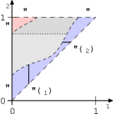
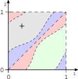
Figure 1: Integration domain in point splitting regularization. The left figure shows the shaded integration domain for two ordered insertions into the Wilson loop. The colored stripe and corner are removed by point splitting. The dotted line depicts how we split up the domain into two convenient integration regions. The right figure illustrates an odd feature of the corner when considering a Yangian level-one generator which acts with opposite signs on the two big triangles. Here the upper corner is in the periodic continuation of the stripe in the lower triangle. Thus in some sense regularization has the opposite effect on the removed stripe and triangle.

The above results on the concrete form of the remainder R𝑅R show that the argument in sec. 5.2 requires proper regularization and potentially renormalization as well. The point is that R𝑅R has a linear UV-divergence which leads to a quadratic divergence for the term d2R12|1=2evaluated-atsubscriptd2subscript𝑅1212\mathrm{d}_{2}R_{12}|_{1=2} in (5.2).

Divergence.

Let us therefore restart the above calculation in point splitting regularization where |τ1τ2|>ε(τ1)=ε¯(τ2)subscript𝜏1subscript𝜏2𝜀subscript𝜏1¯𝜀subscript𝜏2|\tau_{1}-\tau_{2}|>\varepsilon(\tau_{1})=\bar{\varepsilon}(\tau_{2}).181818We will not make further assumptions on the nature of ε𝜀\varepsilon. The simplest choice would be to let the coordinate τ𝜏\tau be proportional to the arc length of the curve and ε=ε¯𝜀¯𝜀\varepsilon=\bar{\varepsilon} be a constant cut-off parameter. However, this choice can obscure some features of renormalization, and we therefore prefer to work with a fairly general scheme where x˙2superscript˙𝑥2\dot{x}^{2} and ε,ε¯𝜀¯𝜀\varepsilon,\bar{\varepsilon} are not assumed to be constant. The full integration domain 0<τ1<τ2<10subscript𝜏1subscript𝜏210<\tau_{1}<\tau_{2}<1 needs to be adjusted not only where τ1τ2subscript𝜏1subscript𝜏2\tau_{1}\approx\tau_{2}, but also at τ10subscript𝜏10\tau_{1}\approx 0, τ21subscript𝜏21\tau_{2}\approx 1 where both points approach each other due to periodicity of the Wilson loop, see fig. 1. We thus obtain for the regularized integral of d1d2R12subscriptd1subscriptd2subscript𝑅12\mathrm{d}_{1}\mathrm{d}_{2}R_{12}

εd1d2R12subscript𝜀subscriptd1subscriptd2subscript𝑅12\displaystyle\int_{\varepsilon}\mathrm{d}_{1}\mathrm{d}_{2}R_{12} =ε1ε¯dτ20τ2ε¯dτ112R12+1ε¯1dτ2τ21+ετ2ε¯dτ112R12absentsuperscriptsubscript𝜀1¯𝜀differential-dsubscript𝜏2superscriptsubscript0subscript𝜏2¯𝜀differential-dsubscript𝜏1subscript1subscript2subscript𝑅12superscriptsubscript1¯𝜀1differential-dsubscript𝜏2superscriptsubscriptsubscript𝜏21𝜀subscript𝜏2¯𝜀differential-dsubscript𝜏1subscript1subscript2subscript𝑅12\displaystyle=\int_{\varepsilon}^{1-\bar{\varepsilon}}\mathrm{d}\tau_{2}\int_{0}^{\tau_{2}-\bar{\varepsilon}}\mathrm{d}\tau_{1}\,\partial_{1}\partial_{2}R_{12}+\int_{1-\bar{\varepsilon}}^{1}\mathrm{d}\tau_{2}\int_{\tau_{2}-1+\varepsilon}^{\tau_{2}-\bar{\varepsilon}}\mathrm{d}\tau_{1}\,\partial_{1}\partial_{2}R_{12}
$\displaystyle=\int_{\varepsilon}^{1-\bar{\varepsilon}}\mathrm{d}\tau\,(\partial_{2}R)(\tau-\bar{\varepsilon},\tau)-\int_{\varepsilon}^{1-\bar{\varepsilon}}\mathrm{d}\tau\,(\partial_{2}R)(0,\tau)$
$\displaystyle\quad+\int_{1-\bar{\varepsilon}}^{1}\mathrm{d}\tau\,(\partial_{2}R)(\tau-\bar{\varepsilon},\tau)-\int_{1-\bar{\varepsilon}}^{1}\mathrm{d}\tau\,(\partial_{2}R)(\tau-1+\varepsilon,\tau)$
$\displaystyle=\int_{0}^{1}\mathrm{d}\tau\,(\partial_{2}R)(\tau-\bar{\varepsilon},\tau)+R(0,\varepsilon)-R(0,-\bar{\varepsilon})$
0εdτ(2R)(τε¯,τ)ε¯0dτ(2R)(τ+ε,τ).superscriptsubscript0𝜀differential-d𝜏subscript2𝑅𝜏¯𝜀𝜏superscriptsubscript¯𝜀0differential-d𝜏subscript2𝑅𝜏𝜀𝜏\displaystyle\quad-\int_{0}^{\varepsilon}\mathrm{d}\tau\,(\partial_{2}R)(\tau-\bar{\varepsilon},\tau)-\int_{-\bar{\varepsilon}}^{0}\mathrm{d}\tau\,(\partial_{2}R)(\tau+\varepsilon,\tau). (5.61)

Again, the bi-local terms have been integrated to a local term and some terms located at the boundary. Note that the boundary terms do contribute non-trivially to the final result; fig. 1 may be helpful in understanding this somewhat counter-intuitive feature: The local term subtracts a particular (divergent) contribution from the integral. The boundary term does the same, however, it resides in the periodic continuation of a region where the Yangian level-one generator (effectively) acts with the opposite sign. Hence the natural extension of the local term to the boundary does not actually absorb the boundary term, but rather reinforces it by a factor of 2.

Regularization.

Let us now expand the contributing terms in the UV-limit ε0𝜀0\varepsilon\to 0.191919Here and in the following it is permissible to consider ε𝜀\varepsilon as a function of τ𝜏\tau and still treat it as an expansion parameter, i.e. it approaches the constant function zero. We find

R(τ,τ+ε)𝑅𝜏𝜏𝜀\displaystyle R(\tau,\tau+\varepsilon) =1εR1(τ)+12R˙1(τ)+R1(τ)ε+𝒪\bBigg@0(ε2\bBigg@0),\displaystyle=\frac{1}{\varepsilon}R_{-1}(\tau)+{\textstyle\frac{1}{2}}\dot{R}_{-1}(\tau)+R_{1}(\tau)\varepsilon+\mathcal{O}\mathopen{\bBigg@{0}}(\varepsilon^{2}\mathclose{\bBigg@{0}}),
(2R)(τ,τ+ε)subscript2𝑅𝜏𝜏𝜀\displaystyle(\partial_{2}R)(\tau,\tau+\varepsilon) =1ε2R1(τ)+R1(τ)+𝒪\bBigg@0(ε\bBigg@0).\displaystyle=-\frac{1}{\varepsilon^{2}}R_{-1}(\tau)+R_{1}(\tau)+\mathcal{O}\mathopen{\bBigg@{0}}(\varepsilon\mathclose{\bBigg@{0}}). (5.62)

Note that the constant term 12R˙1(τ)12subscript˙𝑅1𝜏{\textstyle\frac{1}{2}}\dot{R}_{-1}(\tau) in the ε𝜀\varepsilon-expansion of R(τ,τ+ε)𝑅𝜏𝜏𝜀R(\tau,\tau+\varepsilon) follows from the antisymmetry R(τ1,τ2)=R(τ2,τ1)𝑅subscript𝜏1subscript𝜏2𝑅subscript𝜏2subscript𝜏1R(\tau_{1},\tau_{2})=-R(\tau_{2},\tau_{1}). Inserting these expansions into the above Yangian action one obtains after some careful calculation

εd1d2R12subscript𝜀subscriptd1subscriptd2subscript𝑅12\displaystyle\int_{\varepsilon}\mathrm{d}_{1}\mathrm{d}_{2}R_{12} =01dτ(1+ε˙ε2R1(τ)+R1(τ))+4+2ε˙εR1(0)+𝒪\bBigg@0(ε\bBigg@0).\displaystyle=\int_{0}^{1}\mathrm{d}\tau\,\left(-\frac{1+\dot{\varepsilon}}{\varepsilon^{2}}\,R_{-1}(\tau)+R_{1}(\tau)\right)+\frac{4+2\dot{\varepsilon}}{\varepsilon}\,R_{-1}(0)+\mathcal{O}\mathopen{\bBigg@{0}}(\varepsilon\mathclose{\bBigg@{0}}). (5.63)

Note that for a non-constant function ε𝜀\varepsilon we have to rely on the relationship ε(τ1)=ε¯(τ2)𝜀subscript𝜏1¯𝜀subscript𝜏2\varepsilon(\tau_{1})=\bar{\varepsilon}(\tau_{2}) at the cut-off. This implies the two equivalent relations

ε(τ)=ε¯(τ+ε(τ)),ε¯(τ)=ε(τε¯(τ)),formulae-sequence𝜀𝜏¯𝜀𝜏𝜀𝜏¯𝜀𝜏𝜀𝜏¯𝜀𝜏\varepsilon(\tau)=\bar{\varepsilon}(\tau+\varepsilon(\tau)),\qquad\bar{\varepsilon}(\tau)=\varepsilon(\tau-\bar{\varepsilon}(\tau)), (5.64)

which can be solved perturbatively as

ε¯=εεε˙+εε˙2+12ε2ε¨+𝒪(ε4).¯𝜀𝜀𝜀˙𝜀𝜀superscript˙𝜀212superscript𝜀2¨𝜀𝒪superscript𝜀4\bar{\varepsilon}=\varepsilon-\varepsilon\dot{\varepsilon}+\varepsilon\dot{\varepsilon}^{2}+{\textstyle\frac{1}{2}}\varepsilon^{2}\ddot{\varepsilon}+\mathcal{O}(\varepsilon^{4}). (5.65)

Gladly, all the terms in the bi-local remainder (5.63) can be absorbed by an appropriate regularization of the Yangian action on Wilson loops. As discussed in sec. 2.5, the integral terms can be absorbed by redefining the local action of the Yangian on the gauge field as follows:

(𝕁^𝒜)ε=N2dτ(2R)(τε¯,τ).subscriptsubscript^𝕁𝒜𝜀𝑁2d𝜏subscript2𝑅𝜏¯𝜀𝜏(\widehat{\mathbb{J}}_{*}\mathcal{A})_{\varepsilon}=-\frac{N}{2}\mathrm{d}\tau(\partial_{2}R)(\tau-\bar{\varepsilon},\tau). (5.66)

Note that this action maps an adjoint field to a plain number. Ordinarily one would expect that the gauge structure of the fields is preserved by the action of a symmetry. Nevertheless, here we are in the planar limit where such a rule makes sense (just as the bi-local insertion of the level-one generators). The above local action can be realized on the components of the gauge field as follows202020Other regularization rules are conceivable which involve the fermionic components of the gauge field or which make use of total derivative terms.

(𝕁^𝒜μ)ε=N2pμp2(2R)(τε¯,τ).subscriptsubscript^𝕁subscript𝒜𝜇𝜀𝑁2subscript𝑝𝜇superscript𝑝2subscript2𝑅𝜏¯𝜀𝜏(\widehat{\mathbb{J}}_{*}\mathcal{A}_{\mu})_{\varepsilon}=-\frac{N}{2}\frac{p_{\mu}}{p^{2}}\,(\partial_{2}R)(\tau-\bar{\varepsilon},\tau). (5.67)

For the remaining boundary term in (5.63) we have to adjust the definition of the Yangian action on the Wilson loop (2.41) by a boundary term

(𝕁^κ𝒲)ε=𝒲[(𝕁^κ𝒜)ε]+fκ𝒲ρδ[𝕁δ𝒜;𝕁ρ𝒜]εN(Rκ(0,ε)Rκ(0,ε¯))𝒲.subscriptsuperscriptsubscript^𝕁𝜅𝒲𝜀𝒲delimited-[]subscriptsuperscriptsubscript^𝕁𝜅𝒜𝜀superscript𝑓𝜅subscript𝒲𝜌𝛿subscriptsuperscriptsubscript𝕁𝛿𝒜superscriptsubscript𝕁𝜌𝒜𝜀𝑁superscript𝑅𝜅0𝜀superscript𝑅𝜅0¯𝜀𝒲(\widehat{\mathbb{J}}_{*}^{\kappa}\mathcal{W})_{\varepsilon}=\mathcal{W}\bigl{[}(\widehat{\mathbb{J}}_{*}^{\kappa}\mathcal{A})_{\varepsilon}\bigr{]}+f^{\kappa}{}_{{\rho}{\delta}}\mathcal{W}\bigl{[}\mathbb{J}_{*}^{\delta}\mathcal{A};\mathbb{J}_{*}^{\rho}\mathcal{A}\bigr{]}_{\varepsilon}-N\bigl{(}R^{\kappa}(0,\varepsilon)-R^{\kappa}(0,-\bar{\varepsilon})\bigr{)}\mathcal{W}. (5.68)

Such boundary terms are natural because the boundary is also involved in the regularization of the Wilson loop.

Altogether Yangian symmetry of Wilson loops requires a 1/ε21superscript𝜀21/\varepsilon^{2} divergent local term, a finite local term as well as a 1/ε1𝜀1/\varepsilon divergent boundary term as spelled out in (5.63). The crucial point in favor of Yangian symmetry is that no bi-local and no bulk-boundary counterterms are needed.

Level-one momentum.

For concreteness, we continue with the level-one momentum ^μsuperscriptsubscript^𝜇\widehat{\mathbb{P}}_{*}^{\mu} for which R12[Pμ]subscript𝑅12delimited-[]superscriptP𝜇R_{12}[\mathrm{P}^{\mu}] is given by (5.38) and (5.39). The expansion of this function near coincident points takes the form

R12[P]subscript𝑅12delimited-[]P\displaystyle R_{12}[\mathrm{P}] =2g2π2[2εp1+p1p˙p1\displaystyle=\frac{2g^{2}}{\pi^{2}}\bigg{[}-\frac{2}{\varepsilon}p^{-1}+p^{-1}\dot{p}p^{-1}
+εp1(13p¨+23θ¯¨θ˙23θ¯˙θ¨12p˙p1p˙8θ¯˙θ˙p1θ¯˙θ˙)p1+𝒪(ε2)],\displaystyle\qquad+\varepsilon p^{-1}\Bigl{(}{\textstyle\frac{1}{3}}\ddot{p}+{\textstyle\frac{2}{3}}\ddot{\bar{\theta}}\dot{\theta}-{\textstyle\frac{2}{3}}\dot{\bar{\theta}}\ddot{\theta}-{\textstyle\frac{1}{2}}\dot{p}p^{-1}\dot{p}-8\dot{\bar{\theta}}\dot{\theta}p^{-1}\dot{\bar{\theta}}\dot{\theta}\Bigr{)}p^{-1}+\mathcal{O}(\varepsilon^{2})\biggr{]}, (5.69)

from which the relevant functions $R_{-1}$ and $R_{1}$ can be read off easily.

A curious observation concerns reparametrization of the Wilson loop: The function R1[P]subscript𝑅1delimited-[]PR_{-1}[\mathrm{P}] is covariant under a reparametrization τσ(τ)maps-to𝜏𝜎𝜏\tau\mapsto\sigma(\tau)

R1[P]σ˙R1[P].maps-tosubscript𝑅1delimited-[]P˙𝜎subscript𝑅1delimited-[]PR_{-1}[\mathrm{P}]\mapsto\dot{\sigma}\,R_{-1}[\mathrm{P}]. (5.70)

Together with the transformation dτdτσ˙maps-tod𝜏d𝜏˙𝜎\mathrm{d}\tau\mapsto\mathrm{d}\tau\,\dot{\sigma} of the measure dτd𝜏\mathrm{d}\tau and the transformation εσ˙εmaps-to𝜀˙𝜎𝜀\varepsilon\mapsto\dot{\sigma}\,\varepsilon of the cut-off ε𝜀\varepsilon, the leading contribution dτR1[P]/ε2d𝜏subscript𝑅1delimited-[]Psuperscript𝜀2\mathrm{d}\tau\,R_{-1}[\mathrm{P}]/\varepsilon^{2} to the integrand is invariant. Conversely, the function R1[P]subscript𝑅1delimited-[]PR_{1}[\mathrm{P}] is not covariant,

R1[P]1σ˙(R1[P]+16S(σ)R1[P]),maps-tosubscript𝑅1delimited-[]P1˙𝜎subscript𝑅1delimited-[]P16𝑆𝜎subscript𝑅1delimited-[]PR_{1}[\mathrm{P}]\mapsto\frac{1}{\dot{\sigma}}\,\bigl{(}R_{1}[\mathrm{P}]+{\textstyle\frac{1}{6}}S(\sigma)R_{-1}[\mathrm{P}]\bigr{)}, (5.71)

but rather transforms by the addition of a Schwarzian derivative

S(σ):=σ˙˙˙σ˙32(σ¨σ˙)2assign𝑆𝜎˙˙˙𝜎˙𝜎32superscript¨𝜎˙𝜎2S(\sigma):=\frac{\dddot{\sigma}}{\dot{\sigma}}-\frac{3}{2}\left(\frac{\ddot{\sigma}}{\dot{\sigma}}\right)^{2} (5.72)

multiplying the divergence term R1subscript𝑅1R_{-1}. Given the singularity structure of the function R12subscript𝑅12R_{12}, the appearance of the Schwarzian derivative is natural. Due to this singularity we must consider the transformation of ε𝜀\varepsilon at higher orders in ε𝜀\varepsilon. The exact transformation of ε𝜀\varepsilon reads

ε(τ)σ(τ+ε(τ))σ(τ)=εσ˙+12ε2σ¨+16ε3σ˙˙˙+𝒪(ε4).maps-to𝜀𝜏𝜎𝜏𝜀𝜏𝜎𝜏𝜀˙𝜎12superscript𝜀2¨𝜎16superscript𝜀3˙˙˙𝜎𝒪superscript𝜀4\varepsilon(\tau)\mapsto\sigma(\tau+\varepsilon(\tau))-\sigma(\tau)=\varepsilon\dot{\sigma}+{\textstyle\frac{1}{2}}\varepsilon^{2}\ddot{\sigma}+{\textstyle\frac{1}{6}}\varepsilon^{3}\dddot{\sigma}+\mathcal{O}(\varepsilon^{4}). (5.73)

The relevant combination of divergence terms happens to transform with a Schwarzian derivative as well

1+ε˙ε21σ˙2(1+ε˙ε2+16S(σ)+𝒪(ε)).maps-to1˙𝜀superscript𝜀21superscript˙𝜎21˙𝜀superscript𝜀216𝑆𝜎𝒪𝜀\frac{1+\dot{\varepsilon}}{\varepsilon^{2}}\mapsto\frac{1}{\dot{\sigma}^{2}}\left(\frac{1+\dot{\varepsilon}}{\varepsilon^{2}}+{\textstyle\frac{1}{6}}S(\sigma)+\mathcal{O}(\varepsilon)\right). (5.74)

The extra term multiplying R1subscript𝑅1R_{-1} cancels nicely with the transformation of R1subscript𝑅1R_{1}, and thus the local contributions are properly reparametrization-invariant. Moreover,

1+12ε˙ε1σ˙(1+12ε˙ε),maps-to112˙𝜀𝜀1˙𝜎112˙𝜀𝜀\frac{1+{\textstyle\frac{1}{2}}\dot{\varepsilon}}{\varepsilon}\mapsto\frac{1}{\dot{\sigma}}\left(\frac{1+{\textstyle\frac{1}{2}}\dot{\varepsilon}}{\varepsilon}\right), (5.75)

which implies that the boundary term also stays invariant (but its position is actually shifted).

6 Summary and Conclusions

This work completes the symmetry investigations of the smooth Maldacena–Wilson loops in 𝒩=4𝒩4\mathcal{N}=4 non-chiral superspace started in [13], where we proved global superconformal and local kappa-symmetry of the loop along with establishing the finite result for the vacuum expectation value at first perturbative order for general paths. Here we have investigated the Yangian symmetry of Wilson loops in detail and proved the existence of this hidden symmetry at leading perturbative order. Let us briefly summarize the key results of this work.

The level-one generators of the Y[𝔭𝔰𝔲(2,2|4)]𝑌delimited-[]𝔭𝔰𝔲2conditional24Y[\mathfrak{psu}(2,2|4)] Yangian acting on a Wilson line are represented by a bi-local and a local piece. In order to define the bi-local piece in a gauge-covariant manner, we introduced gauge-covariant conformal generators 𝕁δsuperscriptsubscript𝕁𝛿\mathbb{J}_{*}^{{\delta}}. These act compositely on the gauge fields through a conformal transformation plus a compensating gauge transformation. While the difference to the standard conformal action 𝕁δsuperscript𝕁𝛿\mathbb{J}^{{\delta}} disappears on the vacuum expectation value of a Wilson loop, it does make a crucial difference for the bi-local part of the Yangian level-one generator 𝕁^δsuperscriptsubscript^𝕁𝛿\widehat{\mathbb{J}}_{*}^{{\delta}} where it implements gauge covariance. The local piece of the Yangian level-one generators on the other hand arises from the need to cancel the UV-divergences induced by the action of the bi-local piece in the coincidence limit. We worked out the Yangian invariance at the leading perturbative order in detail in the presence of a point splitting regulator. The form of the local terms was explicitly determined. Moreover, we demonstrated the closure of the level-one algebra and the compatibility of Yangian symmetry with kappa-symmetry. We did not verify the Serre relations for our realization of the Yangian symmetry. However, these relations merely serve to make the algebra smaller. If for some reason they should not hold, the symmetry algebra of the smooth Wilson loops would not be a Yangian, but it would in fact be much bigger. Clarifying this is left to future work.

In fact, we did observe that there is an additional Yangian symmetry, namely the level-one hypercharge, which belongs to Y[𝔲(2,2|4)]𝑌delimited-[]𝔲2conditional24Y[\mathfrak{u}(2,2|4)] rather than Y[𝔭𝔰𝔲(2,2|4)]𝑌delimited-[]𝔭𝔰𝔲2conditional24Y[\mathfrak{psu}(2,2|4)]. This symmetry has been observed before in similar situations [16, 15], and the derivations are analogous to the other level-one generators with minor additional complications.

While we strove to keep the discussion as generic as possible, importantly we saw that the consistency of the Yangian symmetry crucially depended on two properties of the underlying gauge theory: Firstly, the vanishing of the dual Coxeter number of the underlying superconformal symmetry algebra, secondly the existence of a technical G-identity related to the contraction of the field strength two-form with conformal vector fields. Both are fulfilled by 𝒩=4𝒩4\mathcal{N}=4 super Yang–Mills theory and tightly constrain the models to which integrability can possibly apply.

Finally, we would like to stress that at the leading perturbative order the bi-local action of our conformal generators on a correlation function takes the form

fκ𝕁δρδ𝒜1(τ1)𝕁ρ𝒜2(τ2)(1)d1d2R12κ,similar-tosubscriptdelimited-⟨⟩superscript𝑓𝜅subscriptsuperscriptsubscript𝕁𝛿𝜌𝛿subscript𝒜1subscript𝜏1superscriptsubscript𝕁𝜌subscript𝒜2subscript𝜏21subscriptd1subscriptd2subscriptsuperscript𝑅𝜅12\bigl{\langle}f^{{\kappa}}{}_{{\rho}{\delta}}\,\mathbb{J}_{*}^{{\delta}}\mathcal{A}_{1}(\tau_{1})\,\mathbb{J}_{*}^{{\rho}}\mathcal{A}_{2}(\tau_{2})\bigr{\rangle}_{(1)}\sim\mathrm{d}_{1}\mathrm{d}_{2}R^{\kappa}_{12}\,, (6.1)

not necessarily to be inserted into a Wilson loop. Here R12subscript𝑅12R_{12} is the remainder function giving rise to the local piece of the level-one Yangian 𝕁^δsuperscriptsubscript^𝕁𝛿\widehat{\mathbb{J}}_{*}^{{\delta}}. It is interesting to compare this to the conformal symmetry:

𝕁δ𝒜1(τ1)𝒜2(τ2)+𝒜1(τ1)𝕁δ𝒜2(τ2)(1)d1Q12δ+d2Q21δ.similar-tosubscriptdelimited-⟨⟩superscriptsubscript𝕁𝛿subscript𝒜1subscript𝜏1subscript𝒜2subscript𝜏2subscript𝒜1subscript𝜏1superscriptsubscript𝕁𝛿subscript𝒜2subscript𝜏21subscriptd1subscriptsuperscript𝑄𝛿12subscriptd2subscriptsuperscript𝑄𝛿21\bigl{\langle}\mathbb{J}_{*}^{{\delta}}\mathcal{A}_{1}(\tau_{1})\,\mathcal{A}_{2}(\tau_{2})+\mathcal{A}_{1}(\tau_{1})\,\mathbb{J}_{*}^{{\delta}}\mathcal{A}_{2}(\tau_{2})\bigr{\rangle}_{(1)}\sim\mathrm{d}_{1}Q^{\delta}_{12}+\mathrm{d}_{2}Q^{\delta}_{21}. (6.2)

While the level-zero transformations provide only one total derivative, both derivatives in the level-one action are required for Yangian invariance of the Wilson loop. The relation (6.1) might be of future use.

A useful point to mention at the end of our study concerns UV-finiteness: We focused on the special case of kappa-symmetric Maldacena–Wilson loops in order to avoid UV-regularization which might obscure the symmetries. Our derivations and results, however, turn out to be independent of this assumption. Whether or not the Wilson loop is kappa-symmetric, the bi-local insertion of the Yangian level-one generators are UV-divergent and require regularization. Renormalization of the Yangian action removes the undesired terms and makes the Yangian become a symmetry. Thus our result in fact applies to the larger class of generic smooth Wilson loops (1) whose couplings qisuperscript𝑞𝑖q^{i} to the scalars are unconstrained.

In this paper we only discussed a single Wilson loop. What can we say about Yangian symmetry of the expectation value of a product of two Wilson loops, trW1trW2delimited-⟨⟩trsubscript𝑊1trsubscript𝑊2\langle\operatorname{tr}W_{1}\,\operatorname{tr}W_{2}\rangle? At leading order in 1/N1𝑁1/N the expectation value factorizes into the leading orders of the expectation values of the individual Wilson loops. There is nothing new to be learned here. The first sub-leading terms in the 1/N1𝑁1/N expansion are either connected or disconnected. The disconnected terms are non-planar, and Yangian symmetry is most likely spoiled. In any case, this result again follows from a single Wilson loop. The connected term has the large-N𝑁N topology of an annulus. As such it is analogous to the planar two-point function of single trace operators for which integrability made a big difference. This connected term is still expected to be constrained by the center of the Yangian, as explained in ref. [37]. This point deserves further study.

The general smooth super Wilson loop depends on an infinite number of bosonic and fermionic variables. In order to employ the uncovered hidden symmetries towards finding the exact expression for the vacuum expectation value of such operators, it is wise to look at special types of contours depending on a finite number of variables while preserving the smoothness of the curve. In [13] we proposed spline-shaped Wilson loops composed of piecewise-quadratic contours joined in a way ensuring UV-finiteness at the first perturbative order. It would be equally interesting to study situations where UV-singularities arise, namely corners, light-like points or segments as well as self-intersections. These may or may not lead to anomalies or violations of Yangian symmetry. It would be interesting to study such simple super Wilson loops and particular situations thereby putting the uncovered integrability to test and to work.

Acknowledgments.

We thank James Drummond, Nadav Drukker and Hagen Münkler for important discussions. The work of NB is partially supported by grant no. 200021-137616 from the Swiss National Science Foundation, through the SNSF NCCR SwissMAP and by grant no. 615203 from the European Research Council under the FP7. DM gratefully acknowledges the support of the DFG funded Graduate School GK 1504. JP thanks the Pauli Center for Theoretical Studies, Zürich and the Institute for Theoretical Physics at ETH Zürich for hospitality and support in the framework of a visiting professorship. No non-supersymmetric gauge theories were harmed in this investigation.

Appendix A Conventions and Notations

We use the following notations

  • 4d vector indices: $\mu$, $\nu,\rho,\ldots=0,\ldots,3$

  • 4d left spinor indices: $\alpha$, $\beta,\gamma,\ldots=1,2$

  • 4d right spinor indices: $\dot{\alpha}$, $\dot{\beta},\dot{\gamma},\ldots=\dot{1},\dot{2}$

  • 6d vector indices: $i$, $j,k,\ldots=1,\ldots,6$

  • 6d spinor indices: $a$, $b,c,\ldots=1,\ldots,4$

  • 4d $\mathcal{N}=4$ non-chiral superspace: $\{x^{\mu},\theta^{a\alpha},\bar{\theta}^{\dot{\alpha}}{}_{a}\}$

  • 4d 𝒩=4𝒩4\mathcal{N}=4 super connections and scalar superfield: 𝒜μcovsubscriptsuperscript𝒜cov𝜇\mathcal{A}^{\text{cov}}_{\mu}, 𝒜αacovsubscriptsuperscript𝒜cov𝛼𝑎\mathcal{A}^{\text{cov}}_{\alpha a}, 𝒜covaα˙\mathcal{A}^{\text{cov}\,a}{}_{\dot{\alpha}} and ΦisubscriptΦ𝑖\Phi_{i} or ΦabsubscriptΦ𝑎𝑏\Phi_{ab}

  • 4d super-momentum: $p^{\mu}=\dot{x}^{\mu}+\theta\sigma^{\mu}\dot{\bar{\theta}}-\dot{\theta}\sigma^{\mu}\bar{\theta}$

  • Scalar coupling: $q^{i}=n^{i}\sqrt{p^{\mu}p_{\mu}}$ with $q^{i}q^{i}=p^{\mu}p_{\mu}$ and $n^{i}n^{i}=1$

  • Gauge coupling constant: $g$

  • N𝑁N is the rank of the $\mathrm{U}(N)$ gauge group.

We use the mostly minus signature. The four-dimensional Pauli matrices are given by σμ=(𝟏,σ)subscript𝜎𝜇1𝜎\sigma_{\mu}=(\mathbf{1},\vec{\sigma}) and σ¯μ=(𝟏,σ)subscript¯𝜎𝜇1𝜎\bar{\sigma}_{\mu}=(\mathbf{1},-\vec{\sigma}), where

σ1=(0110),σ2=(0ii0),σ3=(1001).formulae-sequencesubscript𝜎1matrix0110formulae-sequencesubscript𝜎2matrix0𝑖𝑖0subscript𝜎3matrix1001\sigma_{1}=\begin{pmatrix}0&1\\ 1&0\end{pmatrix},\qquad\sigma_{2}=\begin{pmatrix}0&-i\\ i&0\end{pmatrix},\qquad\sigma_{3}=\begin{pmatrix}1&0\\ 0&-1\end{pmatrix}. (A.1)

They satisfy the usual algebra

σμσ¯ν+σνσ¯μ=2ημν,σ¯μσν+σ¯νσμ=2ημν.formulae-sequencesubscript𝜎𝜇subscript¯𝜎𝜈subscript𝜎𝜈subscript¯𝜎𝜇2subscript𝜂𝜇𝜈subscript¯𝜎𝜇subscript𝜎𝜈subscript¯𝜎𝜈subscript𝜎𝜇2subscript𝜂𝜇𝜈\sigma_{\mu}\bar{\sigma}_{\nu}+\sigma_{\nu}\bar{\sigma}_{\mu}=2\eta_{\mu\nu},\qquad\bar{\sigma}_{\mu}\sigma_{\nu}+\bar{\sigma}_{\nu}\sigma_{\mu}=2\eta_{\mu\nu}. (A.2)

Here is a list of notations we use for the generators of the superconformal algebra and its Yangian:

  • JJ\mathrm{J} an abstract generator of the superconformal algebra,

  • 𝒥𝒥\mathcal{J} the $(2|4|2)\times(2|4|2)$ matrix representation,

  • 𝐉𝐉\mathbf{J} the representation of $\mathrm{J}$ on the paths,

  • 𝐉^^𝐉\widehat{\mathbf{J}} the level-one Yangian generator corresponding to $\mathbf{J}$,

  • 𝕁𝕁\mathbb{J} a representation of $\mathrm{J}$ on the fields,

  • 𝕁^^𝕁\widehat{\mathbb{J}} the level-one Yangian generator corresponding to $\mathbb{J}$,

  • 𝕁subscript𝕁\mathbb{J}_{*} a different representation of JJ\mathrm{J} on the fields. This maps fields to gauge-covariant fields. It differs from the other representation 𝕁𝕁\mathbb{J} by a gauge transformation.

  • 𝕁^subscript^𝕁\widehat{\mathbb{J}}_{*} the level-one Yangian corresponding to $\mathbb{J}_{*}$,

  • 𝕁^,bisubscript^𝕁bi\widehat{\mathbb{J}}_{*,\text{bi}} the bi-local part of $\widehat{\mathbb{J}}_{*}$.

Appendix B Superconformal Generators

Let us define

𝒵=(x+2θ1),𝒵¯=(12θ¯x).formulae-sequence𝒵matrixsuperscript𝑥2𝜃1¯𝒵matrix12¯𝜃superscript𝑥\mathcal{Z}=\begin{pmatrix}x^{+}\\ 2\theta\\ 1\end{pmatrix},\qquad\overline{\mathcal{Z}}=\begin{pmatrix}-1&-2\bar{\theta}&x^{-}\end{pmatrix}. (B.1)

We have 𝒵¯𝒵=0¯𝒵𝒵0\overline{\mathcal{Z}}\mathcal{Z}=0. A superconformal transformation determined by a (2|4|2)×(2|4|2)242242(2|4|2)\times(2|4|2) supermatrix u𝑢u, acts on the 𝒵𝒵\mathcal{Z} and 𝒵¯¯𝒵\overline{\mathcal{Z}} as follows

δ𝒵=u𝒵+𝒵λ,δ𝒵¯=𝒵¯u+λ¯𝒵¯,formulae-sequence𝛿𝒵𝑢𝒵𝒵𝜆𝛿¯𝒵¯𝒵𝑢¯𝜆¯𝒵\delta\mathcal{Z}=u\mathcal{Z}+\mathcal{Z}\lambda,\qquad\delta\overline{\mathcal{Z}}=-\overline{\mathcal{Z}}u+\overline{\lambda}\overline{\mathcal{Z}}, (B.2)

where λ𝜆\lambda, λ¯¯𝜆\overline{\lambda} are 2×2222\times 2 matrices. Due to these compensating transformations parameterized by λ𝜆\lambda, λ¯¯𝜆\overline{\lambda}, the action of the central charge in 𝔲(2,2|4)𝔲2conditional24\mathfrak{u}(2,2|4) is not well defined. Notice also that the transformations in eq. (B.2) preserve the constraint 𝒵¯𝒵=0¯𝒵𝒵0\overline{\mathcal{Z}}\cdot\mathcal{Z}=0.

A generic element of the super-algebra is represented by the matrix

a𝒫+χ𝒬+χ¯𝒬¯+ω+ω¯¯+r+ρ𝒮+ρ¯𝒮¯+b𝒦=(2ω¯2χ¯2a2ρ¯2r2χ2b2ρ2ω).𝑎𝒫𝜒𝒬¯𝜒¯𝒬superscript𝜔superscriptsuperscript¯𝜔superscript¯superscript𝑟superscript𝜌𝒮¯𝜌¯𝒮𝑏𝒦matrix2superscript¯𝜔2¯𝜒2𝑎2¯𝜌2superscript𝑟2𝜒2𝑏2𝜌2superscript𝜔a\cdot\mathcal{P}+\chi\cdot\mathcal{Q}+\bar{\chi}\cdot\mathcal{\bar{Q}}+\omega^{\prime}\cdot\mathcal{L}^{\prime}+\bar{\omega}^{\prime}\cdot\mathcal{\bar{L}}^{\prime}+r^{\prime}\cdot\mathcal{R}^{\prime}+\rho\cdot\mathcal{S}+\bar{\rho}\cdot\mathcal{\bar{S}}+b\cdot\mathcal{K}=\begin{pmatrix}-2\bar{\omega}^{\prime}&2\bar{\chi}&-2a\\ 2\bar{\rho}&-2r^{\prime}&-2\chi\\ -2b&2\rho&2\omega^{\prime}\end{pmatrix}. (B.3)

The action of the supermatrix u𝑢u yields transformations for the superspace coordinates (x,θ,θ¯)𝑥𝜃¯𝜃(x,\theta,\bar{\theta}), which can be expressed as differential operators. This implies the following representation as differential operators

a𝒫𝑎𝒫\displaystyle a\cdot\mathcal{P} =ax,absent𝑎subscript𝑥\displaystyle=-a\cdot\partial_{x}, (B.4a)
χ𝒬𝜒𝒬\displaystyle\chi\cdot\mathcal{Q} =χθ(θ¯χ)x,absent𝜒subscript𝜃¯𝜃𝜒subscript𝑥\displaystyle=-\chi\cdot\partial_{\theta}-(\bar{\theta}\chi)\cdot\partial_{x}, (B.4b)
χ¯𝒬¯¯𝜒¯𝒬\displaystyle\bar{\chi}\cdot\mathcal{\bar{Q}} =(χ¯θ)xχ¯θ¯,absent¯𝜒𝜃subscript𝑥¯𝜒subscript¯𝜃\displaystyle=(\bar{\chi}\theta)\cdot\partial_{x}-\bar{\chi}\cdot\partial_{\bar{\theta}}, (B.4c)
ω¯¯superscript¯𝜔superscript¯\displaystyle\bar{\omega}^{\prime}\cdot\mathcal{\bar{L}}^{\prime} =(ω¯x)x2(ω¯θ¯)θ¯,absentsuperscript¯𝜔𝑥subscript𝑥2superscript¯𝜔¯𝜃subscript¯𝜃\displaystyle=-(\bar{\omega}^{\prime}x)\cdot\partial_{x}-2(\bar{\omega}^{\prime}\bar{\theta})\cdot\partial_{\bar{\theta}}, (B.4d)
ωsuperscript𝜔superscript\displaystyle\omega^{\prime}\cdot\mathcal{L}^{\prime} =(xω)x2(θω)θ,absent𝑥superscript𝜔subscript𝑥2𝜃superscript𝜔subscript𝜃\displaystyle=-(x\omega^{\prime})\cdot\partial_{x}-2(\theta\omega^{\prime})\cdot\partial_{\theta}, (B.4e)
rsuperscript𝑟superscript\displaystyle r^{\prime}\cdot\mathcal{R}^{\prime} =2(rθ)θ+2(θ¯r)θ¯,absent2superscript𝑟𝜃subscript𝜃2¯𝜃superscript𝑟subscript¯𝜃\displaystyle=-2(r^{\prime}\theta)\cdot\partial_{\theta}+2(\bar{\theta}r^{\prime})\cdot\partial_{\bar{\theta}}, (B.4f)
ρ𝒮𝜌𝒮\displaystyle\rho\cdot\mathcal{S} =(x+ρθ)x4(θρθ)θ+(xρ)θ¯,absentsuperscript𝑥𝜌𝜃subscript𝑥4𝜃𝜌𝜃subscript𝜃superscript𝑥𝜌subscript¯𝜃\displaystyle=-(x^{+}\rho\theta)\cdot\partial_{x}-4(\theta\rho\theta)\cdot\partial_{\theta}+(x^{-}\rho)\cdot\partial_{\bar{\theta}}, (B.4g)
ρ¯𝒮¯¯𝜌¯𝒮\displaystyle\bar{\rho}\cdot\mathcal{\bar{S}} =(θ¯ρ¯x)x+4(θ¯ρ¯θ¯)θ¯+(ρ¯x+)θ,absent¯𝜃¯𝜌superscript𝑥subscript𝑥4¯𝜃¯𝜌¯𝜃subscript¯𝜃¯𝜌superscript𝑥subscript𝜃\displaystyle=(\bar{\theta}\bar{\rho}x^{-})\cdot\partial_{x}+4(\bar{\theta}\bar{\rho}\bar{\theta})\cdot\partial_{\bar{\theta}}+(\bar{\rho}x^{+})\cdot\partial_{\theta}, (B.4h)
b𝒦𝑏𝒦\displaystyle b\cdot\mathcal{K} =12(x+bx++xbx)x+2(xbθ¯)θ¯+2(θbx+)θ,absent12superscript𝑥𝑏superscript𝑥superscript𝑥𝑏superscript𝑥subscript𝑥2superscript𝑥𝑏¯𝜃subscript¯𝜃2𝜃𝑏superscript𝑥subscript𝜃\displaystyle={\textstyle\frac{1}{2}}(x^{+}bx^{+}+x^{-}bx^{-})\cdot\partial_{x}+2(x^{-}b\bar{\theta})\cdot\partial_{\bar{\theta}}+2(\theta bx^{+})\cdot\partial_{\theta}, (B.4i)

where we used the notations ax=aα˙ααα˙𝑎subscript𝑥superscript𝑎˙𝛼𝛼subscript𝛼˙𝛼a\cdot\partial_{x}=a^{\dot{\alpha}\alpha}\partial_{\alpha\dot{\alpha}}, χθ=χaααa𝜒subscript𝜃superscript𝜒𝑎𝛼subscript𝛼𝑎\chi\cdot\partial_{\theta}=\chi^{a\alpha}\partial_{\alpha a}, χ¯θ¯=χ¯α˙¯aaα˙\bar{\chi}\cdot\partial_{\bar{\theta}}=\bar{\chi}^{\dot{\alpha}}{}_{a}\bar{\partial}^{a}{}_{\dot{\alpha}}, etc. We emphasize that these generators only reproduce the action of the superconformal group on the coordinates (x,θ,θ¯)𝑥𝜃¯𝜃(x,\theta,\bar{\theta}); the action on the coordinates q𝑞q is not contained in these expressions.

References