ON THE EVOLUTION OF MAGNETIC WHITE DWARFS

Abstract

We present the first radiation magnetohydrodynamics simulations of the atmosphere of white dwarf stars. We demonstrate that convective energy transfer is seriously impeded by magnetic fields when the plasma-$\beta$ parameter, the thermal to magnetic pressure ratio, becomes smaller than unity. The critical field strength that inhibits convection in the photosphere of white dwarfs is in the range $B=1$-50 kG, which is much smaller than the typical 1-1000 MG field strengths observed in magnetic white dwarfs, implying that these objects have radiative atmospheres. We have then employed evolutionary models to study the cooling process of high-field magnetic white dwarfs, where convection is entirely suppressed during the full evolution ($B\gtrsim 10$ MG). We find that the inhibition of convection has no effect on cooling rates until the effective temperature ($T_{\rm eff}$) reaches a value of around 5500 K. In this regime, the standard convective sequences start to deviate from the ones without convection owing to the convective coupling between the outer layers and the degenerate reservoir of thermal energy. Since no magnetic white dwarfs are currently known at the low temperatures where this coupling significantly changes the evolution, effects of magnetism on cooling rates are not expected to be observed. This result contrasts with a recent suggestion that magnetic white dwarfs with $T_{\rm eff}\lesssim 10,000$ K cool significantly slower than non-magnetic degenerates.

1. INTRODUCTION

Magnetic white dwarfs are stellar remnants featuring global magnetic structures with field strengths from 1 kG to 1000 MG. They account for a significant part of the white dwarf population with an estimated fraction of around 10% in volume complete samples (Liebert et al. 2003; Schmidt et al. 2003; Kawka et al. 2007). Most of these objects are high-field magnetic white dwarfs (HFMWD), with field strengths $B>1$ MG, and a distribution of magnetic field strengths that appears to peak around $\sim 20$ MG (Schmidt et al. 2003; Külebi et al. 2009). HFMWDs show obvious Zeeman line splitting in spectroscopic observations. It is currently difficult to understand these data owing to the lack of an appropriate theory of Stark broadening in the presence of a background magnetic field in an arbitrary direction (Main et al. 1998). In particular, the standard spectroscopic technique employed to derive atmospheric parameters from the Balmer lines (Bergeron et al. 1992) can not be used to constrain the mass and cooling age of HFMWDs (Külebi et al. 2009). However, there is a growing sample of HFMWDs in common proper motion pairs or with known trigonometric parallaxes, allowing to derive masses. This sample shows a mean mass of $\sim 0.80$ $M_{\odot}$ (Ferrario et al. 2015; Briggs et al. 2015), which is significantly higher than the mean mass of non-magnetic white dwarfs ($\sim 0.60$ $M_{\odot}$, see, e.g., Kleinman et al. 2013).

Numerous recent studies have provided scenarios for the origin of HFMWDs, accounting for their mass, velocity, and magnetic field strength distributions. The lack of a significant trend in the number of HFMWDs as a function of atmospheric composition and cooling age (Külebi et al. 2009), as well the presence of field strengths too large to be produced by a convective dynamo (Dufour et al. 2008), suggest that magnetic fields are remnants of the white dwarf progenitors. Current scenarios tend to be grouped in three categories, suggesting that HFMWDs are: remnants of intermediate mass stars with conserved fossil fields (Angel et al. 1981; Wickramasinghe & Ferrario 2005); the outcome of mergers of either two white dwarfs or a white dwarf and the core of a giant star (García-Berro et al. 2012; Külebi et al. 2013a; Wickramasinghe et al. 2014; Briggs et al. 2015); or products of the amplification of a seed field by a convective dynamo in the core of the evolved progenitors (Ruderman & Sutherland 1973; Kissin & Thompson 2015). The origin of magnetic white dwarfs remains elusive since current observations do not allow to clearly differentiate between these evolution channels. Magnetic white dwarfs in clusters and common proper motion pairs (Külebi et al. 2010; Dobbie et al. 2012; Külebi et al. 2013b; Dobbie et al. 2013) are consistent with single star evolution in some but not all cases. It is also difficult to explain the white dwarfs with the strongest magnetic fields, as well as the absence of HFMWDs with late-type star companions, without invoking the merger scenario (Wickramasinghe et al. 2014; Kissin & Thompson 2015).

On the other hand, weaker magnetic fields ($B\lesssim 1$ MG) are also found in white dwarfs, although they are difficult to detect systematically owing to the lack of obvious Zeeman splitting in high-resolution spectra for $B\lesssim$ 20 kG (Jordan et al. 2007). A few small spectropolarimetric surveys, sensitive to field strengths as small as $\sim$1 kG, have put the fraction of kG-range white dwarfs at 3-30%, with a roughly constant 1-10% incidence per decade of magnetic field strength (Jordan et al. 2007; Landstreet et al. 2012; Kawka & Vennes 2012). The uncertain ratio reflects the small number statistics in the current samples. These magnetic white dwarfs appear to have average masses and are thought to origin from single stellar evolution (Jordan et al. 2007), with the magnetic fields possibly generated through a dynamo process in the white dwarf progenitor (Wickramasinghe et al. 2014). Furthermore, large observed values for $\langle B_{\rm z}\rangle/\langle|B|\rangle$ are a strong indicator that the fields have a global organized structure, unlike the complex magnetic fields at the surface of Sun-like stars (Landstreet et al. 2012).

Gaia will provide precise parallaxes for more than 100,000 white dwarfs, including all known magnetic white dwarfs (Torres et al. 2005; Carrasco et al. 2014), and spectroscopic follow-ups will identify even more magnetic objects. Gaia will establish the first homogeneous mass distribution and cooling sequence of magnetic remnants. Given the ubiquitous presence of magnetic white dwarfs in the high-mass regime, it is critical to understand these objects to recover the Galactic star formation history and initial mass function in the $\sim 3$-8 $M_{\odot}$ range (Tremblay et al. 2014). Magnetic remnants can also be used to constrain stellar evolution at intermediate masses (Külebi et al. 2013b) and study possible populations of mergers (Badenes & Maoz 2012; Wegg & Phinney 2012). It is therefore essential, at this stage, to build precise model atmospheres and evolution sequences for these peculiar degenerate stars. It has been suggested for a long time that convection is completely inhibited in HFMWDs (Wickramasinghe & Martin 1986; Valyavin et al. 2014), although this has not yet been verified with realistic simulations. Furthermore, Kepler et al. (2013) suggest that small undetected magnetic fields could impact the mass distribution of cool convective white dwarfs.

Valyavin et al. (2014) have recently proposed that the inhibition of convection in magnetic white dwarfs has a large impact on cooling rates, by increasing the cooling times by a factor of two to three. However, they arrived at this conclusion with a simple analytical argument and it needs to be verified with state-of-the-art evolution models. In this work, we perform the first radiation magnetohydrodynamics (RMHD) simulations of the atmosphere of magnetic pure-hydrogen (DA) white dwarfs (Section 2.1). We then consider the results of these simulations for the computation of new cooling sequences for magnetic white dwarfs using an established evolution code (Section 2.2). We discuss the implications of these results in Section 3 and conclude in Section 4.

2. WHITE DWARF MODELS

2.1. Magnetohydrodynamics Simulations

We have computed RMHD simulations with the CO⁵BOLD code (Freytag et al. 2012) for pure-hydrogen DA white dwarfs. We rely on a representative set of atmospheric parameters, $T_{\rm eff}\sim 10,000$ K and a surface gravity of $\log g=8.0$, and our simulations are detailed in Table 1. The setup of the simulations is very similar to that of the non-magnetic models presented in Tremblay et al. (2013a, b). In the temperature regime considered here, the convection zone is significantly deeper than the atmospheric layers, and we use a bottom boundary (at Rosseland optical depth $\tau_{\rm R}\sim 10^{3}$) open to convective flows and radiation, where a zero net mass flux is ensured. We fix the entropy of the ascending material at 2.0819 erg g^-1 K^-1 for all simulations, corresponding to the value in the non-magnetic simulation at $T_{\rm eff}=10,025$ K and $\log g=8.0$ from Tremblay et al. (2013b). The lateral boundaries are periodic, and the top boundary is open to material flows and radiation. We rely on the same opacities, equation of state, and grid resolution ($150\times 150\times 150$) as the previous non-magnetic simulations. The frequency dependent, i.e. non-gray, radiative transfer is solved along long characteristics employing Feautrier’s method. Opacities are grouped into bins (for details on the opacity binning approach see, e.g., Nordlund 1982; Ludwig et al. 1994; Vögler et al. 2004) using the 8-bin scheme of Tremblay et al. (2013b).

The main difference compared to earlier computations is that we have imposed, at the start of the simulations, a vertically oriented magnetic field (towards the exterior of the star) with an amplitude of 0.5 kG and 5 kG for our two magnetic simulations, respectively. The magnetic boundary conditions are imposed independently to the hydrodynamics conditions. We require that magnetic field lines remain vertical at both the top and bottom layers, while lateral boundaries are periodic. We further require that the magnetic flux is constant at the bottom, mimicking the effect of a global fossil field anchored in the deep degenerate core. We note that our RMHD simulations do not assume hydrostatic equilibrium and automatically take into account the turbulent pressure, magnetic tension forces, and magnetic pressure.

Table 1RMHD Models of White Dwarfs

$T_{\rm eff}$	$\log g$	$x$	$z$	$z(\tau_{\rm R}=1)-z_{\rm bot}$	$B_{\rm z}$	$B_{\rm z,rms}(\tau_{\rm R}=1)$	$\delta I_{\rm rms}/\langle I\rangle$	Mach$(\tau_{\rm R}=1)$
(K)	(cm s-2)	(km)	(km)	(km)	(kG)	(kG)	(%)
10024	8.0	2.11	0.83	0.38	0	0	14.69	0.45
10037	8.0	2.11	0.83	0.38	0.5	1.28	14.13	0.38
9147	8.0	2.11	0.63	0.30	5.0	5.38	21.86	0.25

Note. — All quantities were averaged over 250 snapshots and over constant geometrical depth when appropriate. $T_{\rm eff}$ is derived from the temporal and spatial average of the emergent flux. $B_{\rm z}$ is the horizontally averaged magnetic field, which is constant at all times and all depths from the requirement of magnetic flux conservation. $B_{\rm z,rms}$ is the rms vertical magnetic field at the geometrical depth that corresponds to $\langle\tau_{\rm R}\rangle_{\rm x,y}=1$. $\delta I_{\rm rms}/\langle I\rangle$ is the relative intensity contrast (see Eq. (73) of Freytag et al. 2012).

The MHD module of CO⁵BOLD (see Section 3.7 of Freytag et al. 2012) provides several numerical methods for solving the MHD equations, which are quite different from the ones employed for pure hydrodynamics. In particular, the method used here relies on the HLL solver (Harten et al. 1983), which is more stable but with increased dissipation compared to the Roe solver used for the published grid of DA white dwarfs. The MHD module also enforces the divergence-free condition $\nabla\cdot B=0$ based on a constrained transport scheme (see, e.g., Tóth 2000). In order to study the effect of magnetic fields on the atmospheric stratification, we have computed a third model with the same MHD solver but no magnetic field. We computed all simulations for five seconds in stellar time, which is several times the convective turnover timescale.

Figure 1 presents snapshots of the emergent intensity for our three relaxed simulations. From an average over 125 snapshots, we also display at the top of the panels the $T_{\rm eff}$ values (derived from the emergent flux) and the relative intensity contrast. We observe that magnetic fields have a significant impact on the emergent intensity. For $B_{\rm z}=0.5$ kG, diverging upflows concentrate magnetic flux in downflows, much like what is observed in the so-called quiet regions on the Sun (Nordlund et al. 2009), which are characterized by a rather weak average magnetic flux. Small magnetic flux concentrations form and appear as bright intergranular points since they act as radiative leak due to their reduced mass density. Table 1 demonstrates that the root-mean-square vertical magnetic field in the photosphere is significantly larger than the average magnetic field owing to these flux concentrations. For a field strength of $B_{\rm z}=5$ kG, convection is already largely inhibited, and occurs as narrow and bright plumes very similarly to Sun spots where $B\gtrsim 2.5$ kG (Weiss et al. 1996; Schüssler & Vögler 2006). This is not a surprising result since the thermal pressure in the photosphere of the simulated white dwarfs is only slightly larger than that in the Sun, and a similar magnetic pressure is necessary to inhibit convective flows. Studies of the impact of magnetic fields on surface convection in the Sun and Sun-like stars by numerous RMHD simulations (Rempel et al. 2009; Cheung et al. 2010; Freytag et al. 2012; Beeck et al. 2013; Steiner et al. 2014) can also be used to learn about the same process in white dwarfs, even though the origin and large scale structure of magnetic fields are very different.

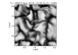
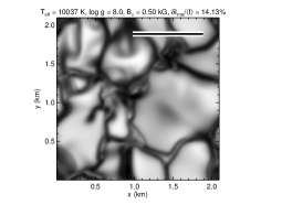
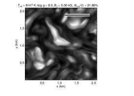
Figure 1.— Bolometric intensity emerging from the $xy$ plane at the top of computational domain for CO⁵BOLD 3D simulations computed with the MHD solver. All simulations have a constant surface gravity of $\log g=8.0$, a pure-hydrogen composition, and rely on the same entropy value for the inflowing material through the open bottom boundary. The simulations shown in the middle and right panels have at the bottom an imposed average vertical magnetic field of 0.5 kG and 5 kG, respectively. The rms intensity contrast with respect to the mean intensity and $T_{\rm eff}$ values are also shown above the panels. The length of the bar in the top right is 10 times the pressure scale height at $\tau_{\rm R}=2/3$.

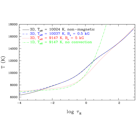
Figure 2.— Temperature structure as function of optical depth (logarithmic scale) for the non-magnetic (black), 0.5 kG (blue), and 5 kG (red) 3D RMHD simulations. The temperature was determined from an average of $\langle T^{4}\rangle$ over surfaces of constant optical depth. We also show a purely radiative 1D model atmosphere (green), where convection was artificially suppressed, at the same $T_{\rm eff}$ value as the 5 kG model.

Figure 2 presents the temperature profiles of our simulations, drawn from the average of $\langle T^{4}\rangle$ over surfaces of constant $\tau_{\rm R}$ for 12 snapshots. For the 0.5 kG simulation, we observe that the magnetic field only has an impact on the upper photosphere ($\tau_{\rm R}<10^{-2}$), where the temperature gradient is shallower. The importance of the feedback effect of magnetic fields on the stellar structure can be estimated from the plasma-$\beta$ parameter

$$\beta=\frac{8\pi P}{B^{2}}~{},$$ (1)

the thermal to magnetic pressure ratio, where $P$ is the thermal pressure, and $B$ the average magnetic field strength. Since the thermal pressure is rapidly decreasing with height while the magnetic pressure is roughly constant, magnetic feedback effects increase with height. There are two main reasons for the shallower temperature gradient in the uppermost stable layers of magnetic white dwarfs. First of all, magnetic field lines restrain convective flows, hence the convective overshoot that usually cools the upper layers is weaker (Tremblay et al. 2013a). This is a purely dynamical effect that will not be observed in a 1D magnetic model with local convection. Furthermore, the radiative heating, magnetic dissipation, and magnetic pressure all contribute to increase the thermal pressure scale height compared to the non-magnetic case, which implies a shallower temperature gradient as a function of geometrical depth. In general, the consequence is also a shallower temperature gradient as a function of $\tau_{\rm R}$.

For a field strength of 5 kG, the overall atmospheric stratification is significantly impacted by the presence of a magnetic field. Convective energy transfer is impeded in the photosphere and Figure 3 demonstrates that the convective flux at $\tau_{\rm R}$ = 1 is reduced by a factor of two compared to the non-magnetic model. The smaller convective energy transfer implies that the stratification in the convectively unstable regions must adjust to a steeper temperature gradient to transport the same amount of total flux. The temperature gradient in the line-forming regions becomes very close to the radiative gradient, as demonstrated in Figure 2 from the comparison with a 1D structure where convection was artificially suppressed. On the other hand, in the deeper layers where the thermal energy is larger, convection is still significant for this field strength. Nevertheless, the steeper temperature gradient in the upper convectively unstable layers ($\tau_{\rm R}\gtrsim 0.1$), caused by the inhibition of convection, decreases the $T_{\rm eff}$ value by 880 K for the same conditions at the bottom. Full evolutionary calculations are necessary to link the magnetic atmospheres to the stellar interior, and this result does not imply that magnetic white dwarfs have smaller luminosities for the same core temperature (see Section 2.2). For our models at $T_{\rm eff}\sim$ 10,000 K and $\log g$ = 8.0, $\beta$ = 1 for $B\sim$ 5.7 kG at the photosphere ($\tau_{\rm R}$ = 1). This critical field strength is very close to the observed transition between a convective and an almost fully radiative temperature gradient in the RMHD simulations. Our results support the suggestion that when the plasma-$\beta$ is smaller than unity, i.e. when the magnetic pressure dominates over the thermal energy, the white dwarf atmospheric stratification adjusts to a radiative gradient since convective energy transfer is significantly hampered.

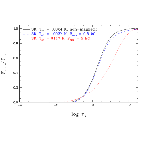
Figure 3.— Ratio of the convective to total energy flux as a function of optical depth (logarithmic scale) for the non-magnetic (black), 0.5 kG (blue), and 5 kG (red) 3D RMHD simulations. The $\langle$3D$\rangle$ convective flux is the sum of the enthalpy and kinetic energy fluxes (see Eq. 5 of Tremblay et al. 2015) averaged over constant geometrical depth.

In those cases where the plasma-$\beta$ parameter is smaller than unity, the atmosphere is not expected to become static or homogeneous since the stratification is still convectively unstable, albeit unable to create energetically efficient convective flows. In particular, the relative intensity contrast for the $B$ = 5 kG simulation is still 21.9%, an even larger value than for the non-magnetic simulation. While convection is restricted to narrow and inefficient plumes, the temperature contrast and velocities in those structures are still large. It is currently unclear how these fluctuations would decrease as the magnetic field strength is further increased. It is a serious technical challenge to compute RMHD simulations with larger field strengths since the time steps are dictated by the Alfvén speed $B/\sqrt{4\pi\rho}$, where $\rho$ is the density. For instance, the simulation at 5 kG is already of the order of 10 times slower than the non-magnetic simulation. Finally, the magnetic field tends to form localized flux concentrations in the intergranular lanes, and the spatial resolution of our RMHD simulations likely needs to be improved in order to properly characterize the intensity contrast and small-scale fluctuations.

We have employed a standard grid of 1D model atmospheres (Tremblay et al. 2011) to compute the critical magnetic field strength, defined by $\beta=1$, above which convection is significantly suppressed in the photosphere ($\tau_{R}=1$). Figure 4 shows that the critical field is always below $\sim$50 kG. Known magnetic white dwarfs have field strengths typically much larger than these values, and our results suggest that convection is suppressed at the surface of HFMWDs. Furthermore, while we have only performed simulations with a vertically oriented magnetic field, it is generally thought that the damping of convection is even stronger for horizontally oriented fields since the Lorentz force will act against vertical flows. In other words, convection is expected to be globally inhibited above a certain magnetic field strength (Valyavin et al. 2014).

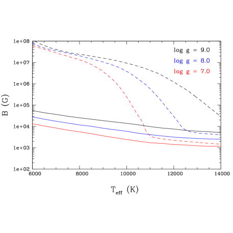
Figure 4.— Magnetic field strength that corresponds to plasma-$\beta=1$ in the photosphere ($\tau_{\rm R}=1$, solid lines) and base of the convection zone (dashed lines) as a function of $T_{\rm eff}$. Sequences are color-coded for $\log g$ = 7.0 (red), 8.0 (blue), and 9.0 (black), from bottom to top. Plasma-$\beta=1$ estimates when convective energy transfer is suppressed by the magnetic field. Photospheric values are derived from 1D model atmospheres with a mixing-length parameterization of ML2/$\alpha$ = 0.8 (Tremblay et al. 2011) while values for the base of the convection zone are derived from standard envelope models using a slightly more efficient ML2/$\alpha$ = 1.0 convection (Fontaine et al. 2001).

The rapid increase of $\beta$ as a function of depth implies that when convection is suppressed at the surface, it could still be fully developed in deeper layers as demonstrated by our 5 kG simulation. Once $\beta$ = 1 at the base of the convection zone, the entire convection zone is likely to be significantly disrupted. Figure 4 shows this critical field strength (dashed lines) as predicted by 1D envelopes (Fontaine et al. 2001). In the intermediate regime between the suppression of convection at the surface and in the full convection zone, one should use radiative atmospheres but consider the possibility of an internal convection zone. However, new cooling sequences with partial convective inhibition would need to be computed to determine the size and structure of these internal convection zones. These calculations are outside the scope of this work because a realistic magnetic field geometry would be required to properly model individual white dwarfs. Furthermore, it is difficult to extrapolate our RMHD results for the atmosphere, where convective velocities are close to the sound speed, to deeper convective layers where the flows have a kinetic energy density that becomes far smaller than the thermal energy density. Once the magnetic field becomes larger than the kinetic equipartition field strength

$$B_{\rm eq}^{2}/8\pi=\frac{1}{2}\langle\rho v_{\rm conv}^{2}\rangle~{},$$ (2)

where $v_{\rm conv}$ is the local convective velocity, different modes of convection with smaller physical scales may set in. Figure 5 demonstrates that the kinetic equipartition field strength is in the kG-range throughout the convection zone for a representative 0.6 $M_{\odot}$ white dwarf. It suggests that convection could be disrupted for magnetic field strengths smaller than those defined by the conservative $\beta=1$ estimate of Figure 4 for the bottom of the convection zone.

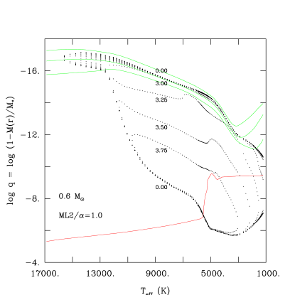
Figure 5.— Contours of kinetic equipartition magnetic field strength (logarithmic values in Gauss identified on the panel, see Eq. (2)) as a function of fractional mass $\log q=\log(1-M(r)/M_{*})$ integrated from the surface and $T_{\rm eff}$. We rely on the evolution sequence at 0.6 $M_{\odot}$ with ML2/$\alpha$ = 1.0 convection (see Section 2.2). We also show the position of three atmospheric layers ($\tau_{\rm R}$ = 0.1, 1.0, 10.0, from top to bottom in solid green lines) and the degeneracy boundary ($\eta$ = 0, solid red line).

2.2. Evolutionary Models

It has been known for a long time that superficial convection has no influence whatsoever on the cooling time until the base of the convection zone reaches into the degenerate reservoir of thermal energy and couples, for the first time in the cooling process, the surface with that reservoir (Tassoul et al. 1990; Fontaine et al. 2001). The convective coupling occurs at $T_{\rm eff}$ values lower than 6000 K in white dwarfs, hence the suppression of convection is not expected to impact cooling rates for warmer remnants. This argument contradicts the suggestion from Valyavin et al. (2014, see Fig. 3a) that the suppression of convection changes the cooling rates and explains the observed temperature distribution of magnetic white dwarfs, for which their coolest bin is at $T_{\rm eff}=6000$ K. To demonstrate it quantitatively, this section presents new evolution sequences that we have computed with our state-of-the-art white dwarf evolutionary code (Fontaine et al. 2001, 2013). To fully appreciate the results, we also review the important properties of white dwarf cooling in Section 2.3.

We computed a standard 0.6 $M_{\odot}$ sequence with a C/O core, a helium envelope containing 10^-2 of the total mass, and a hydrogen outer layer containing 10^-4 of the total mass. In particular, it takes into account superficial convection as it develops with time relying on the so-called ML2/$\alpha$ = 1.0 version of the mixing-length theory (Böhm & Cassinelli 1971; Tassoul et al. 1990). We have computed an additional sequence where convection is totally suppressed, thus mimicking the maximum possible effect of magnetic inhibition, e.g. for field strengths of 10 MG or larger according to Figure 4. Both sequences are presented in Figure 6 (left panel), where the solid curves refer to the normal sequence, while the dotted curves refer to the “magnetic” sequence. The location of convective coupling is indicated by the first dashed vertical segment from the left. This corresponds specifically to the model with the base of its convection zone first entering the degenerate thermal reservoir from above (the upper boundary of that reservoir is defined by a local value of the electron degeneracy parameter of $\eta$ = 0, where $\eta kT$ is the chemical potential of the free electrons). When convective coupling occurs, $T_{\rm eff}=$ 5527 K and the cooling age is 3.13 Gyr. Above $T_{\rm eff}$ = 5527 K, there is no significant difference whatsoever between the behaviors of the two sequences, meaning that magnetic inhibition of superficial convection does nothing to the cooling process in this hotter phase. We have also computed sequences at 1.0 $M_{\odot}$ which are likely more representative of the HFMWDs. Figure 6 (right) demonstrates that the behavior is similar to the lower mass case, and convective coupling takes place at a only slightly higher temperature.

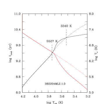
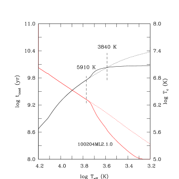
Figure 6.— (Left:) cooling sequences in terms of cooling time (black, left axis) and central temperature (red, right axis) as a function of decreasing $T_{\rm eff}$ for a 0.6 $M_{\odot}$ DA white dwarf (solid lines). We have assumed thick helium and hydrogen layers with fractional masses of 10^-2 and 10^-4, respectively. We have also computed a sequence where convection was artificially suppressed mimicking the effect of a strong magnetic field (dotted lines). Convection has no effect on the cooling until there is a convective coupling with the degenerate core at the position illustrated by the first dashed vertical segment from the left. The location where the cooling times become larger for the magnetic sequence is indicated by the second dashed vertical segment from the left. The $T_{\rm eff}$ values for both transitions are shown on the panel. (Right:) same as left panel but for a 1.0 $M_{\odot}$ DA white dwarf.

Our evolutionary sequences demonstrate that the cooling rates, hence the relation between core and surface temperature, must remain the same for magnetic and non-magnetic white dwarfs. We now try to reconcile this fact with the prediction from our RMHD simulations indicating that the inhibition of convection by a magnetic field creates a steeper (radiative) temperature gradient in the outer convectively unstable layers. Figure 7 presents the temperature profile of a model at $T_{\rm eff}\sim 6200$ K from the standard evolution sequence at 0.6 $M_{\odot}$, along with the case where convection was suppressed for the entire cooling process. It confirms that even though there is a much steeper gradient at the surface of magnetic white dwarfs, this is not the case for all internal layers, and the non-magnetic relation between core and (average) surface temperature holds. Interestingly, Figure 8 demonstrates that for the magnetic case, the steep radiative gradient in the outer layers is associated with a very sharp opacity peak as a function of fractional mass. It is unclear if such opacity peak could generate pulsations in magnetic white dwarfs, which we discuss in Section 3.4.

Figure 7.— Temperature structure as a function of fractional mass (both logarithmic values) for a DA white dwarf at $T_{\rm eff}\sim$ 6200 K and 0.6 M_⊙. The solid sequence ($T_{\rm eff}$ = 6243 K) relies on 1D convection (ML2/$\alpha$ = 1.0) while the dotted sequence ($T_{\rm eff}$ = 6205 K) had convection suppressed in the entire cooling process.

Figure 8.— Similar to Figure 7 but for the Rosseland mean opacity ($\kappa$) as a function of fractional mass (both logarithmic values). The solid sequence ($T_{\rm eff}$ = 6243 K) relies on 1D convection (ML2/$\alpha$ = 1.0) while the dotted sequence ($T_{\rm eff}$ = 6205 K) had convection suppressed in the entire cooling process.

2.3. The Cooling Process in White Dwarfs

We have designed Figure 9 to review the cooling process in white dwarfs. The cooling time depends on the amount of thermal energy contained in the star and the rate with which this energy is transferred from the thermal reservoir to the surface. The available thermal energy at a given epoch is given by the integral shown on the y-axis of Figure 9. Here, we show the running integral (black dotted curve), from the center to the surface, for three models belonging to the standard (convective) evolutionary sequence at 0.6 $M_{\odot}$ discussed above. The x-axis shows the fractional mass $\log q=\log(1-M(r)/M_{*})$ integrated from the surface. The upper boundary of the reservoir of thermal energy is a concept that is a bit fuzzy, but it must correspond to a location on the flat part of each curve, i.e., to a layer above which there is practically no more contribution to the reservoir. Conveniently, this boundary is usually defined as the layer where the degeneracy parameter $\eta=0$. In Figure 9, the layer $\eta=0$ corresponds, for each model, to the location of the sharp cutoff on the left of the blue spike. With cooling, the boundary $\eta=0$ moves up toward the surface because the star becomes globally increasingly more degenerate. Moreover, we have illustrated in red the profile of the ratio of the convective flux to total flux, $F_{\rm conv}/F_{\rm tot}$. It should be understood that convective coupling arises when the base of the convection zone reaches the boundary $\eta=0$, which is imminent but has not yet occurred in the coolest model ($T_{\rm eff}$ = 5585 K) shown in the plot. In this particular evolutionary sequence, convective coupling occurs when the star has cooled down to the somewhat lower value of $T_{\rm eff}=5527$ K.

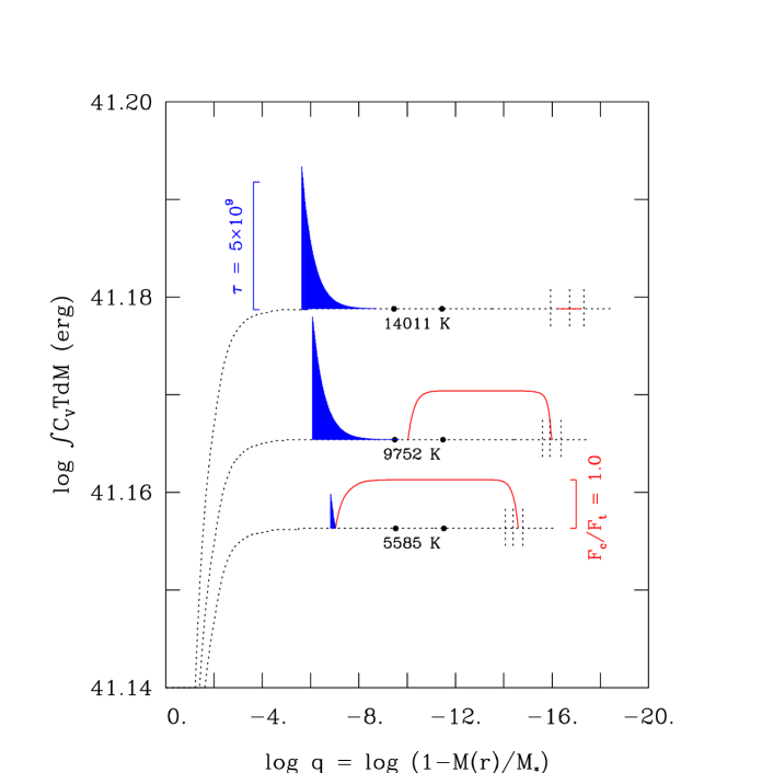
Figure 9.— Logarithmic value of the available thermal energy integrated from the center (left to right, black dotted curves) at three given epochs of the standard 0.6 $M_{\odot}$ cooling sequence ($T_{\rm eff}$ = 14011 K, 9752 K, and 5585 K, identified on the panel) within a certain fractional mass $\log q$. The uppermost degenerate layer ($\eta=0$) corresponds, for each model, to the location of the sharp cutoff on the left of the blue spike. The blue spikes correspond to the running integral of the optical depth, from the base of the convection zone on the right to the layer where $\eta=0$ on the left, with a scale of $\tau_{\rm R}=5\times 10^{9}$. The ratio of the convective to total flux is illustrated by the red profiles (ML2/$\alpha$ = 1.0) and the two black dots on each curve indicate, respectively, the depth where the magnetic pressure is equal to the gas pressure assuming a magnetic field of 10 MG (on the left) and 1 MG (on the right). We also indicate the location of three atmospheric layers along the x-axis, corresponding to $\tau_{\rm R}$ = 10, 1, and 0.1, from left to right (the short vertical dotted line segments).

In a cooling white dwarf, the degenerate core and reservoir of thermal energy is relatively well insulated by a nondegenerate envelope whose global opacity regulates the rate of energy loss. To illustrate this opacity barrier, and in particular the role of the insulating layers between the base of the outer convection zone and the reservoir, we integrated the optical depth ${\rm d}\tau_{\rm R}=-\kappa\rho{\rm d}r$ between the base of the convection zone and the layer $\eta$ = 0. For each model considered, we plotted in Figure 9 in blue the running integral of optical depth, from right to left together with a scale of $\tau_{\rm R}=5\times 10^{9}$. The blue spikes thus identify the layers that are of importance in the insulating process and in the role of regulator of the rate of energy transfer from the core to the surface. Even for the coolest model illustrated here, the opacity barrier is still enormous and the reservoir remains relatively well insulated. The convective coupling will occur in a somewhat cooler phase for which the base of the convection zone finally reaches the boundary $\eta=0$. From that point on in time, the reservoir becomes effectively coupled directly to the atmospheric layers via a convection zone whose efficiency reaches practically 100%. For the first time in the evolution of the star, the exact physical conditions characterizing the atmospheric layers will start playing a role in the cooling process.

The layers where the blue optical depth curve is flat in Figure 9 have a negligible contribution to the opacity barrier and, thus, cannot play any role in the cooling process. For example, for the two warmest models, all of the layers above $\log(1-M(r)/M_{*})\sim-9$ have no impact on this process. For the coolest model, all of the layers above $\log(1-M(r)/M_{*})\sim-7$ have no impact either; the insulating layer represented by the small blue spike is still extremely efficient at regulating by itself the outflow of energy. In this context, we have added in the figure two black dots on each curve which indicate, respectively, the depth where the magnetic pressure is equal to the gas pressure assuming a magnetic field of 10 MG (on the left) and 1 MG (on the right). These layers sit far above the opacity barrier, hence magnetic effects, namely magnetic pressure, may impact the actual stratification of these outer layers, but these layers play no role in the cooling process. They have negligible contribution to the energy reservoir and negligible contribution to the opacity barrier.

A last view on convective coupling can be made from Figure 10 with the standard convective cooling sequence at 0.6 $M_{\odot}$. The small dots represent the opacity contours, while the bold dots represent the convective layers. The opacity maximum is caused by hydrogen recombination. We also show the position of the degeneracy boundary ($\eta$ = 0) with a solid red curve. It is observed that when the degeneracy boundary crosses the convection zone, there is a radical change in the envelope stratification, and conductive transfer dominates for regions below the degeneracy boundary. Figure 6 also demonstrates that for both the 0.6 and 1.0 $M_{\odot}$ cases, the cooling time of the normal convective sequence becomes larger than that of the magnetic sequence in the phase following the onset of convective coupling, while the central temperature immediately drops below that of the magnetic model. This behavior has been explained by Tassoul et al. (1990) and Fontaine et al. (2001), and it is perhaps best understood with the analogy of a warm oven. Convective coupling is like opening the door of the oven; there is initially an excess of heat coming out of the oven, while the inside temperature drops immediately. In a white dwarf undergoing convective coupling, the excess of thermal energy is translated into a delay in the cooling process and the cooling time increases accordingly. After this excess energy has been radiated away, convective coupling enters a second phase, and that is that of accelerated cooling because convection now couples for good the energy reservoir and the surface, and it transfers energy at a greater rate than radiation alone could do. It is thus only in this second phase of the process that the cooling time of the magnetic sequence becomes larger than the cooling time of the normal sequence, as suggested by Valyavin et al. (2014). In Figure 6, the vertical dashed line segments, marked $T_{\rm eff}$ = 3340 and 3840 K for the 0.6 and 1.0 $M_{\odot}$ models, respectively, indicate the very low $T_{\rm eff}$ values below which this second phase can proceed.

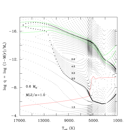
Figure 10.— Opacity contours (small dots, logarithmic values in cm² g^-1 identified on the panel) in the envelope of a 0.6 $M_{\odot}$ white dwarf as a function of fractional mass (logarithmic scale) and $T_{\rm eff}$. We rely on the standard convective sequence with ML2/$\alpha$ = 1.0, and the convection zone is illustrated by the bold dotted contours. We also show the position of three atmospheric layers ($\tau_{\rm R}$ = 0.1, 1.0, 10.0, from top to bottom in solid green lines) and the degeneracy boundary ($\eta$ = 0, solid red line).

We conclude this section with a comparison to the cooling process in magnetized neutron stars, which is also regulated by a heat blanketing envelope between the atmosphere and the stellar interior (see, e.g., Potekhin et al. 2005). For these objects, thermal conduction is the dominant energy transfer mechanism in the degenerate electron gas within the insulating layers, and it has been established that the suppression of thermal conduction in the direction transverse to the magnetic field lines can influence the cooling rates (Hernquist 1985; Potekhin et al. 2007). In a white dwarf, however, the insulating region is non-degenerate and thermal conduction only takes place in the stellar interior, where changes in the conduction rates are unlikely to impact the cooling process. Average magnetic fields are also much weaker in white dwarfs in comparison to magnetized neutron stars.

2.4. Magnetic Effects on Structures

Figure 11 compares the gas and magnetic pressure for a characteristic structure at 0.6 $M_{\odot}$ and $T_{\rm eff}\sim 9750$ K. We assume a 10 MG field at the surface and a conservation of the magnetic flux $4\pi Br^{2}$ in the interior. This is obviously a rough description of the actual magnetic geometry in the interior, which is poorly constrained by observations. Nevertheless, it demonstrates that magnetic effects could only play a role in the outer layers and at the very center, although there is no evidence that magnetic field lines reach the central region. For the illustrated model, a fractional mass depth of $\log(1-M(r)/M_{*})=-9$ corresponds approximately to a fractional radius of $\log(1-r/R_{*})=-2.3$. Thus, magnetic fields (at the 10 MG level) could at best only in the outermost 0.5% of the radius have an influence on the structure of these representative white dwarf models. As a consequence, we conclude that current mass-radius relations for non-magnetic white dwarfs will hold for magnetic remnants as well.

Figure 11.— Thermal pressure profile (solid line) of a DA white dwarf structure at 0.6 $M_{\odot}$ and $T_{\rm eff}$ = 9752 K, the same model as on the middle panel of Figure 9. We also show the magnetic pressure (dotted line) for a field strength of 10 MG at the surface and assuming the conservation of the magnetic flux in the interior.

3. DISCUSSION

The computation of RMHD simulations for DA white dwarfs confirms that convective energy transport is seriously impeded by magnetic field lines when the plasma-$\beta$ parameter is smaller than unity. As a consequence, radiative 1D model atmospheres can be employed for magnetic white dwarfs with $B\gtrsim$ 50 kG according to Figure 4. The main shortcoming in the modeling of most known magnetic white dwarfs remains the spectral synthesis of the Balmer lines accounting for both Stark and Zeeman effects (Wickramasinghe & Martin 1986).

3.1. Photometric Variability of Magnetic White Dwarfs

It is difficult to explain from our results the large number of magnetic white dwarfs that show photometric variations of a few percent over their rotation period (Brinkworth et al. 2013; Lawrie et al. 2013; Valyavin et al. 2014). We have demonstrated in Section 2.2 that the partial or total suppression of convection is unable to change the average surface temperature until there is coupling between the convection zone and the degenerate core at low $T_{\rm eff}$ values. As a consequence, we can not naturally explain global emergent intensity variations for the $T_{\rm eff}$ values of known magnetic white dwarfs. However, we note that if the magnetic field is moving at the surface, as hypothesized by Valyavin et al. (2011) for WD 1953$-$011, the envelope would take some time to adjust to the new surface conditions. The Kelvin-Helmholtz timescale of the portion of the envelope including the entire convection zone is one estimate for this thermal relaxation time, which varies from about one second at 12,000 K to about 1000 yr at 6000 K. Since the cooling rates must remain constant according to our evolutionary models, the flux fluctuations created from this mechanism would average out over the full surface but not necessarily over the apparent stellar disk.

We note that photometric variations are observed in hot magnetic white dwarfs where no convection is predicted, hence it is already clear that convective effects are not involved in some cases. Previously supplied explanations for photometric variations remain valid, such as magneto-optical effects involving radiative transfer under different polarizations (Martin & Wickramasinghe 1979; Wickramasinghe & Martin 1986; Ferrario et al. 1997). Finally, variations are also observed, although with a weaker amplitude, in apparently non-magnetic white dwarfs, where accretion hot spots or UV flux fluctuations and fluorescent optical re-emission have been suggested as possible explanations (Maoz et al. 2015).

3.2. Cooling Age Distribution of Magnetic White Dwarfs

Our results do not support the hypothesis that the observed distribution of HFMWDs as a function of $T_{\rm eff}$ can be explained by different cooling timescales between magnetic and non-magnetic white dwarfs. This does not imply that the number ratio of magnetic to non-magnetic remnants should be constant as a function of $T_{\rm eff}$. The cooling age distribution of HFMWDs could be different from the fact alone that they have a distinct mass distribution. A variation of the velocity distribution as a function of both mass and $T_{\rm eff}$ (Wegg & Phinney 2012), a consequence of the different main-sequence lifetimes, could change the magnetic incidence as a function of $T_{\rm eff}$ even for volume-complete samples. Furthermore, a distinction between magnetic and non-magnetic objects could be present if a significant fraction of magnetic white dwarfs originate from mergers, which presumably have a different cooling history compared to single remnants. Finally, very cool DA white dwarfs have deep convection zones, and for $T_{\rm eff}\lesssim 6000$ K, they reach a regime where the convective turnover timescale at the base of the convection zone is of the order of a few hours, which is similar to the rotation periods of magnetic white dwarfs (Brinkworth et al. 2013). The hypothesis of a $\alpha\omega$ convective dynamo becomes tantalizing, although this needs to be tested with dynamical models. However, this dynamo is unlikely to generate fields stronger than the kinetic equipartition field strength (Fontaine et al. 1973; Thomas et al. 1995; Dufour et al. 2008). Figure 5 demonstrates that for our standard evolutionary sequence at 0.6 $M_{\odot}$, the equipartition field strength reaches a maximum value of $B_{\rm eq}\sim 10$ kG at the base of the convection zone, suggesting it is an unlikely scenario for the known magnetic white dwarfs.

We have found no firm evidence in the literature for a variation in the incidence of magnetic white dwarfs as a function of $T_{\rm eff}$, which differs from the claim of Valyavin et al. (2014) that the picture has now been settled. On the contrary, Liebert et al. (2003), Hollands et al. (2015), and Ferrario et al. (2015) suggest that variations still need to be confirmed owing to several observational biases and conflicting results. Furthermore, Külebi et al. (2009) and Kepler et al. (2013) find no clear evidence of variations in the homogeneous SDSS sample, although most objects have $T_{\rm eff}>7000$ K, above the temperature where Valyavin et al. (2014) observe a significant increase. There is marginal evidence from the local 20 pc sample (Giammichele et al. 2012) that the incidence of magnetic fields increases for $T_{\rm eff}<$ 6000 K. If we consider only DA white dwarfs as well as objects with a derived distance under 20 pc in Table 2 of Giammichele et al. (2012), we find a magnetic incidence of $22\pm 11$% (4 magnetic objects) for 5000 $<T_{\rm eff}$ (K) $<$ 6000, while the value is $10\pm 5$% for warmer objects. We believe it is necessary to confirm this behavior with larger samples to fully understand the evolution of magnetic white dwarfs.

3.3. Magnetic Fields in the White Dwarf Population

Few magnetic white dwarfs have precise atmospheric parameter determinations, and it is typical to exclude them from the samples employed to derive the mean properties of field white dwarfs (see, e.g., Tremblay et al. 2011). It is however difficult to detect magnetic objects with $B\lesssim$ 1 MG at low spectral resolution, hence it is therefore nearly impossible to define clean non-magnetic samples.

We have shown that magnetic fields of a few kG can significantly impact the thermal stratification in the upper layers of convective DA white dwarfs. Yet these fields are too weak to produce any significant Zeeman splitting, hence white dwarfs harboring such fields would not easily be detected. Kepler et al. (2013) have suggested that undetected magnetic fields could explain the so-called high-$\log g$ problem observed in the white dwarf mass distributions (Bergeron et al. 1990). On the other hand, it was recently demonstrated that this problem is instead caused by inaccuracies in the 1D mixing-length convection model (Tremblay et al. 2013b). Furthermore, Kepler et al. (2013) suggest that field strengths increase for convective objects, which would be a manifestation of the amplification of magnetic fields by convection. However, all their observations have $B>1$ MG, which is too strong to be amplified by convection since the kinetic equipartition field strength is always much smaller than $B=1$ MG as demonstrated in Figure 5.

To understand the effects of a population of white dwarfs with small undetected magnetic fields, we have computed synthetic 1D spectra at $T_{\rm eff}=10,000$ K and $\log g$ = 8.0. The spectra are derived from both a standard convective model atmosphere with ML2/$\alpha=0.8$ (Tremblay et al. 2011), and a radiative atmosphere where convection was completely inhibited, mimicking the effect of a weak $5\lesssim B$ (kG) $\lesssim 100$ magnetic field, i.e. the range where Zeeman splitting is negligible at low spectral resolution. The left panel of Figure 12 demonstrates that the predicted Balmer lines of the two models are significantly different, although when projecting the magnetic model on a grid of convective models on the right panel of Figure 12, the Balmer lines look much alike, albeit with an offset in the atmospheric parameters. It implies that it would be difficult to identify such a small magnetic field from spectroscopy alone. This could have an impact on the observed mass distribution of cool convective white dwarfs, although the $\log g$ shift is moderate according to Figure 12, and the incidence of magnetic white dwarfs in the $\sim$ 10 kG-range is expected to be small (Kawka & Vennes 2012; Landstreet et al. 2012).

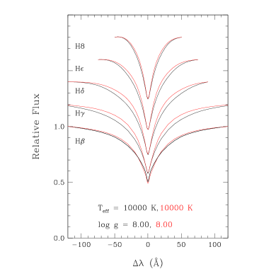
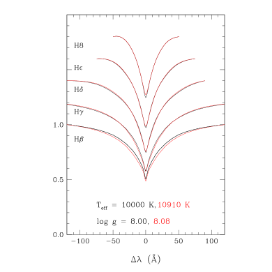
Figure 12.— Left: Predicted Balmer line profiles for a DA white dwarf at $T_{\rm eff}=10,000$ K and $\log g=$ 8.0. The spectra were computed from a standard 1D model atmosphere with ML2$/\alpha$ = 0.8 convection (red) and a radiative 1D atmosphere where convection was artificially suppressed (black), representing the effect of a $B\gtrsim 5$ kG magnetic field. All profiles are normalized to a unity continuum and the transitions are identified on the panel. We have employed a convolution of 3 Å (FWHM) to represent typical observations. Right: Similar to left panel but we show the standard convective 1D model spectra (red, $T_{\rm eff}=10,910$ K and $\log g=8.08$) that best fits the radiative model. It suggests that fitting this magnetic white dwarf with a proper radiative model would result in $\Delta\log g=-0.08$ and $\Delta T_{\rm eff}=-$910 K compared to the standard convective solution.

The situation is different when accounting for 3D effects. In that more realistic case, the magnetic field inhibits convective overshoot so that the upper layers ($\tau_{\rm R}\lesssim 10^{-2}$) must be in radiative equilibrium (see Figure 2). In 1D, these upper layers are never convective and always in radiative equilibrium. As a consequence, synthetic spectral line cores based on 3D simulations are significantly shallower in the magnetic case, while they do not change in 1D. We refrain from a quantitative prediction at this stage since the 3D RMHD structures have been computed with different numerical parameters in comparison to the published 3D grid. Nevertheless, it is a potential explanation for the problem observed in Tremblay et al. (2013b), where the predicted 3D line cores are systematically too deep and suggest that the upper layers are too cool. Figure 2 illustrates that a field strength of $\sim$ 1 kG is sufficient to significantly heat the upper layers.

It is unlikely that the commonly proposed evolution scenarios for magnetic white dwarfs could systematically generate $\sim$ 1 kG magnetic fields, which would then impact the observed line cores. A plausible alternative, however, is that a turbulent dynamo systematically generates weak magnetic fields in convective white dwarfs, a well discussed scenario for quiet regions of the Sun (Cattaneo 1999; Vögler & Schüssler 2007; Moll et al. 2011). It consists of the amplification of small seed magnetic fields by the electrically conducting turbulent convective flows at the surface. Such fields are likely to reach an equilibrium strength of a fraction of the kinetic equipartition energy, corresponding to 0.1-1 kG in the photosphere of convective DA white dwarfs according to Figure 5. The magnetic fields would have characteristic dimensions of the convective eddies of at most a few hundred meters, hence it would be difficult to detect them, except from their systematic feedback effect on the atmospheric stratification. As a consequence, recent spectropolarimetric surveys provide no direct constraint on this scenario. We hope to compute turbulent dynamo RMHD simulations in the future to verify whether the magnetic fields reach a sufficient amplitude to solve the discrepancy between the predicted 3D line cores and observations.

3.4. Pulsating White Dwarfs

It is difficult to apply our results quantitatively to pulsating white dwarfs. The base of the convection zone corresponds to the driving region of the ZZ Ceti pulsations (see, e.g., Fontaine & Brassard 2008), hence the dashed lines in Figure 4 illustrate the critical field where convective energy transfer will be largely suppressed in these layers. Thus, magnetic fields stronger than 1 MG will likely have a dramatic effect on the driving mechanism of the pulsations, although it is difficult to rule out pulsating instabilities at this stage since the stratification will still be unstable. Another aspect of the problem is that the inhibition of convection will create a strong temperature gradient and opacity peak in the convectively unstable upper layers (see Figure 8), which could independently drive pulsations through a $\kappa$-type mechanism. This process has already been suggested for pulsating and strongly magnetic hot DQ white dwarfs (Dufour et al. 2008).

It is difficult to predict the position of an instability strip for magnetic white dwarfs since it is likely to depend on the strength and geometry of the magnetic fields. Indeed, magnetic pressure will impact the position of the opacity peak as function of the radius. We note that the Lorentz force affects nonradial pulsations as well (Saio 2013), requiring additional theoretical work to model pulsating magnetic white dwarfs. However, the Ohmic timescale in the outer layers is short, suggesting that the magnetic field could be relaxed to a force-free potential state. This further highlights the fact that one must rely on realistic magnetic field geometries to model pulsations in magnetic white dwarfs.

For DA atmospheres, MG-range fields are excluded for the 56 bright ZZ Ceti white dwarfs in the Gianninas et al. (2011) sample, suggesting that magnetic fields inhibit pulsations. On the other hand, none of the HFMWDs with known $T_{\rm eff}$ and $\log g$ (Briggs et al. 2015) are within the ZZ Ceti instability strip, an essential ingredient to conclude about the possibility of HFMWD ZZ Ceti white dwarfs.

4. CONCLUSION

We have computed the first RMHD simulations of pure-hydrogen white dwarf atmospheres. We have demonstrated that convective energy transfer is largely suppressed in the atmosphere of magnetic white dwarfs for field strengths larger than $B\sim 50$ kG, confirming quantitatively the previously widespread idea that HFMWDs have no surface convection. Stronger magnetic fields are necessary to fully suppress convection in the envelope, and we find that for $B$ = 1-100 MG, depending on the atmospheric parameters, the full stratification becomes radiative. For intermediate field strengths, the suppression of convection in the upper layers will change the stellar structure in a complex way, and new calculations with partial convective inhibition and realistic magnetic field configurations must be performed to better understand these objects.

We have presented new evolutionary calculations for DA white dwarfs where convection was fully suppressed, e.g. mimicking the effect of a $B\gtrsim 10$ MG field. We find that the suppression of convection has no impact on the cooling rates until there is a convective coupling between the convection zone and the degenerate core in the standard sequence at $T_{\rm eff}\sim$ 5500 K. The currently known magnetic remnants, which are almost all above this temperature, are thus cooling like non-magnetic white dwarfs. Our results also suggest that the effect of magnetic pressure on the mass-radius relation is at most of the order of 1%. Finally, we conclude that the photometric variations observed in a large fraction of magnetic white dwarfs remain largely unexplained.

References

- Angel et al. (1981) Angel, J. R. P., Borra, E. F., & Landstreet, J. D. 1981, ApJS, 45, 457
- Badenes & Maoz (2012) Badenes, C., & Maoz, D. 2012, ApJ, 749, LL11
- Beeck et al. (2013) Beeck, B., Cameron, R. H., Reiners, A., & Schüssler, M. 2013, A&A, 558, AA48
- Bergeron et al. (1990) Bergeron, P., Wesemael, F., Fontaine, G., & Liebert, J. 1990, ApJ, 351, L21
- Bergeron et al. (1992) Bergeron, P., Saffer, R. A., & Liebert, J. 1992, ApJ, 394, 228
- Böhm & Cassinelli (1971) Böhm, K. H., & Cassinelli, J. 1971, A&A, 12, 21
- Briggs et al. (2015) Briggs, G. P., Ferrario, L., Tout, C. A., Wickramasinghe, D. T., & Hurley, J. R. 2015, MNRAS, 447, 1713
- Brinkworth et al. (2013) Brinkworth, C. S., Burleigh, M. R., Lawrie, K., Marsh, T. R., & Knigge, C. 2013, ApJ, 773, 47
- Cattaneo (1999) Cattaneo, F. 1999, ApJ, 515, L39
- Carrasco et al. (2014) Carrasco, J. M., Catalán, S., Jordi, C., et al. 2014, A&A, 565, AA11
- Cheung et al. (2010) Cheung, M. C. M., Rempel, M., Title, A. M., & Schüssler, M. 2010, ApJ, 720, 233
- Dobbie et al. (2012) Dobbie, P. D., Baxter, R., Külebi, B., et al. 2012, MNRAS, 421, 202
- Dobbie et al. (2013) Dobbie, P. D., Külebi, B., Casewell, S. L., et al. 2013, MNRAS, 428, L16
- Dufour et al. (2008) Dufour, P., Fontaine, G., Liebert, J., Williams, K., & Lai, D. K. 2008, ApJ, 683, L167
- Ferrario et al. (2015) Ferrario, L., de Martino, D., Gaensicke, B. T. 2015, Space Sci. Rev., 27
- Ferrario et al. (1997) Ferrario, L., Vennes, S., Wickramasinghe, D. T., Bailey, J. A., & Christian, D. J. 1997, MNRAS, 292, 205
- Fontaine & Brassard (2008) Fontaine, G., & Brassard, P. 2008, PASP, 120, 1043
- Fontaine et al. (1973) Fontaine, G., Thomas, J. H., & van Horn, H. M. 1973, ApJ, 184, 911
- Fontaine et al. (2001) Fontaine, G., Brassard, P., & Bergeron, P. 2001, PASP, 113, 409
- Fontaine et al. (2013) Fontaine, G., Brassard, P., Charpinet, S., Randall, S.K., & Van Grootel, V. 2013, in EPJ Web of Conferences 43, 40th Liège International Astrophysical Colloquium, ed. J. Montalbán, A. Noels & V. Van Grootel (Paris, EDP), 05001
- Freytag et al. (2012) Freytag, B., Steffen, M., Ludwig, H.-G., et al. 2012, Journal of Computational Physics, 231, 919
- García-Berro et al. (2012) García-Berro, E., Lorén-Aguilar, P., Aznar-Siguán, G., et al. 2012, ApJ, 749, 25
- Gianninas et al. (2011) Gianninas, A., Bergeron, P., & Ruiz, M. T. 2011, ApJ, 743, 138
- Giammichele et al. (2012) Giammichele, N., Bergeron, P., & Dufour, P. 2012, ApJS, 199, 29
- Harten et al. (1983) Harten, A., Lax, P. D., & van Leer, B. 1983, SIAM Rev., 25, 35
- Hernquist (1985) Hernquist, L. 1985, MNRAS, 213, 313
- Hollands et al. (2015) Hollands, M., Gaensicke, B., & Koester, D. 2015, arXiv:1503.03866
- Ji et al. (2013) Ji, S., Fisher, R. T., García-Berro, E., et al. 2013, ApJ, 773, 136
- Jordan et al. (2007) Jordan, S., Aznar Cuadrado, R., Napiwotzki, R., Schmid, H. M., & Solanki, S. K. 2007, A&A, 462, 1097
- Kawka et al. (2007) Kawka, A., Vennes, S., Schmidt, G. D., Wickramasinghe, D. T., & Koch, R. 2007, ApJ, 654, 499
- Kawka & Vennes (2012) Kawka, A., & Vennes, S. 2012, MNRAS, 425, 1394
- Kepler et al. (2013) Kepler, S. O., Pelisoli, I., Jordan, S., et al. 2013, MNRAS, 429, 2934
- Kissin & Thompson (2015) Kissin, Y., & Thompson, C. 2015, arXiv:1501.07197
- Kleinman et al. (2013) Kleinman, S. J., Kepler, S. O., Koester, D., et al. 2013, ApJS, 204, 5
- Külebi et al. (2009) Külebi, B., Jordan, S., Euchner, F., Gänsicke, B. T., & Hirsch, H. 2009, A&A, 506, 1341
- Külebi et al. (2010) Külebi, B., Jordan, S., Nelan, E., Bastian, U., & Altmann, M. 2010, A&A, 524, AA36
- Külebi et al. (2013a) Külebi, B., Ekşi, K. Y., Lorén-Aguilar, P., Isern, J., & García-Berro, E. 2013a, MNRAS, 431, 2778
- Külebi et al. (2013b) Külebi, B., Kalirai, J., Jordan, S., & Euchner, F. 2013b, A&A, 554, AA18
- Landstreet et al. (2012) Landstreet, J. D., Bagnulo, S., Valyavin, G. G., et al. 2012, A&A, 545, AA30
- Lawrie et al. (2013) Lawrie, K. A., Burleigh, M. R., Dufour, P., & Hodgkin, S. T. 2013, MNRAS, 433, 1599
- Liebert et al. (2003) Liebert, J., Bergeron, P., & Holberg, J. B. 2003, AJ, 125, 348
- Ludwig et al. (1994) Ludwig, H.-G., Jordan, S., & Steffen, M. 1994, A&A, 284, 105
- Main et al. (1998) Main, J., Schwacke, M., & Wunner, G. 1998, Phys. Rev. A, 57, 1149
- Maoz et al. (2015) Maoz, D., Mazeh, T., & McQuillan, A. 2015, MNRAS, 447, 1749
- Martin & Wickramasinghe (1979) Martin, B., & Wickramasinghe, D. T. 1979, MNRAS, 189, 69
- Moll et al. (2011) Moll, R., Pietarila Graham, J., Pratt, J., et al. 2011, ApJ, 736, 36
- Nordlund (1982) Nordlund, Å. 1982, A&A, 107, 1
- Nordlund et al. (2009) Nordlund, Å., Stein, R. F., & Asplund, M. 2009, Living Reviews in Solar Physics, 6, 2
- Potekhin et al. (2005) Potekhin, A. Y., Urpin, V., & Chabrier, G. 2005, A&A, 443, 1025
- Potekhin et al. (2007) Potekhin, A. Y., Chabrier, G., & Yakovlev, D. G. 2007, Ap&SS, 308, 353
- Rempel et al. (2009) Rempel, M., Schüssler, M., & Knölker, M. 2009, ApJ, 691, 640
- Ruderman & Sutherland (1973) Ruderman, M. A., & Sutherland, P. G. 1973, Nature Physical Science, 246, 93
- Saio (2013) Saio, H. 2013, in EPJ Web of Conferences 43, 40th Liège International Astrophysical Colloquium, ed. J. Montalbán, A. Noels & V. Van Grootel (Paris, EDP), 05005
- Schmidt et al. (2003) Schmidt, G. D., Harris, H. C., Liebert, J., et al. 2003, ApJ, 595, 1101
- Schüssler & Vögler (2006) Schüssler, M., Vögler, A. 2006, ApJ, 641, L73
- Steiner et al. (2014) Steiner, O., Salhab, R., Freytag, B., et al. 2014, PASJ, 66, S5
- Tassoul et al. (1990) Tassoul, M., Fontaine, G., & Winget, D. E. 1990, ApJS, 72, 335
- Thomas et al. (1995) Thomas, J. H., Markiel, J. A., & van Horn, H. M. 1995, ApJ, 453, 403
- Torres et al. (2005) Torres, S., García-Berro, E., Isern, J., & Figueras, F. 2005, MNRAS, 360, 1381
- Tóth (2000) Tóth, G. 2000, Journal of Computational Physics, 161, 605
- Tremblay et al. (2011) Tremblay, P.-E., Bergeron, P., & Gianninas, A. 2011, ApJ, 730, 128
- Tremblay et al. (2013a) Tremblay, P.-E., Ludwig, H.-G., Steffen, M., & Freytag, B. 2013a, A&A, 552, AA13
- Tremblay et al. (2013b) Tremblay, P.-E., Ludwig, H.-G., Steffen, M., & Freytag, B. 2013b, A&A, 559, AA104
- Tremblay et al. (2014) Tremblay, P.-E., Kalirai, J. S., Soderblom, D. R., Cignoni, M., & Cummings, J. 2014, ApJ, 791, 92
- Tremblay et al. (2015) Tremblay, P.-E., Ludwig, H.-G., Freytag, B., et al. 2015, ApJ, 799, 142
- Valyavin et al. (2011) Valyavin, G., Antonyuk, K., Plachinda, S., et al. 2011, ApJ, 734, 17
- Valyavin et al. (2014) Valyavin, G., Shulyak, D., Wade, G. A., et al. 2014, Nature, 515, 88
- Vögler & Schüssler (2007) Vögler, A., & Schüssler, M. 2007, A&A, 465, L43
- Vögler et al. (2004) Vögler, A., Bruls, J. H. M. J., & Schüssler, M. 2004, A&A, 421, 741
- Wegg & Phinney (2012) Wegg, C., & Phinney, E. S. 2012, MNRAS, 426, 427
- Weiss et al. (1996) Weiss, N. O., Brownjohn, D. P., Matthews, P. C., & Proctor, M. R. E. 1996, MNRAS, 283, 1153
- Wickramasinghe & Martin (1986) Wickramasinghe, D. T., & Martin, B. 1986, MNRAS, 223, 323
- Wickramasinghe & Ferrario (2005) Wickramasinghe, D. T., & Ferrario, L. 2005, MNRAS, 356, 1576
- Wickramasinghe et al. (2014) Wickramasinghe, D. T., Tout, C. A., & Ferrario, L. 2014, MNRAS, 437, 675