Computing the Rectilinear Center of Uncertain Points in the Plane

Abstract

In this paper, we consider the rectilinear one-center problem on uncertain points in the plane. In this problem, we are given a set $\mathcal{P}$ of $n$ (weighted) uncertain points in the plane and each uncertain point has $m$ possible locations each associated with a probability for the point appearing at that location. The goal is to find a point $q^{*}$ in the plane which minimizes the maximum expected rectilinear distance from $q^{*}$ to all uncertain points of $\mathcal{P}$, and $q^{*}$ is called a rectilinear center. We present an algorithm that solves the problem in $O(mn)$ time. Since the input size of the problem is $\Theta(mn)$, our algorithm is optimal.

1 Introduction

In the real world, data is inherently uncertain due to many facts, such as the measurement inaccuracy, sampling discrepancy, resource limitation, and so on. A large amount of work has recently been done on uncertain data, e.g., [1, 2, 3, 9, 12, 13, 17, 18]. In this paper, we study the one-center problem on uncertain points in the plane with respect to the rectilinear distance.

Let $\mathcal{P}=\{P_{1},P_{2},\ldots,P_{n}\}$ be a set of $n$ uncertain points in the plane, where each uncertain point $P_{i}\in\mathcal{P}$ has $m$ possible locations $p_{i1},p_{i2},\cdots,p_{im}$ and for each $1\leq j\leq m$, $p_{ij}$ is associated with a probability $f_{ij}\geq 0$ for $P_{i}$ being at $p_{ij}$ (which is independent of other locations).

For any (deterministic) point $p$ in the plane, we use $x_{p}$ and $y_{p}$ to denote the $x$- and $y$-coordinates of $p$, respectively. For any two points $p$ and $q$, we use $d(p,q)$ to denote the rectilinear distance between $p$ and $q$, i.e., $d(p,q)=|x_{p}-x_{q}|+|y_{p}-y_{q}|$.

Consider a point $q$ in the plane. For any uncertain point $P_{i}\in\mathcal{P}$, the expected rectilinear distance between $q$ and $P_{i}$ is defined as

$$\mathsf{E}\mathrm{d}(P_{i},q)=\sum_{j=1}^{m}f_{ij}\cdot d(p_{ij},q).$$

Let $\mathsf{E}\mathrm{d}_{\max}(q)=\max_{P_{i}\in\mathcal{P}}\mathsf{E}\mathrm{d}(P_{i},q)$. A point $q^{*}$ is called a rectilinear center of $\mathcal{P}$ if it minimizes the value $\mathsf{E}\mathrm{d}_{\max}(q^{*})$ among all points in the plane. Our goal is to compute $q^{*}$. Note that such a point $q^{*}$ may not be unique, in which case we let $q^{*}$ denote an arbitrary such point.

We assume that for each uncertain point $P_{i}$ of $\mathcal{P}$, its $m$ locations are given in two sorted lists, one by $x$-coordinates and the other by $y$-coordinates. To the best of our knowledge, this problem has not been studied before. In this paper, we present an $O(mn)$ time algorithm. Since the input size of the problem is $\Theta(nm)$, our algorithm essentially runs in linear time, which is optimal.

Further, our algorithm is applicable to the weighted version of this problem in which each $P_{i}\in\mathcal{P}$ has a weight $w_{i}\geq 0$ and the weighted expected distance, i.e., $w_{i}\cdot\mathsf{E}\mathrm{d}(P_{i},q)$, is considered. To solve the weighted version, we can first reduce it to the unweighted version by changing each $f_{ij}$ to $w_{i}\cdot f_{ij}$ for all $1\leq i\leq n$ and $1\leq j\leq m$, and then apply our algorithm for the unweighted version. The running time is still $O(mn)$.

1.1 Related Work

The problem of finding one-center among uncertain points on a line has been considered in our previous work [21], where an $O(nm)$ time algorithm was given. An algorithm for computing $k$ centers for general $k$ was also given in [21] with the running time $O(mn\log mn+n\log n\log k)$. In fact, in [21] we considered the $k$-center problem under a more general uncertain model where each uncertain point can appear in $m$ intervals. We also studied the one-center problem for uncertain points on tree networks in [20], where a linear-time algorithm was proposed.

There is also a lot of other work on facility location problems for uncertain data. For instances, Cormode and McGregor [7] proved that the $k$-center problem on uncertain points each associated with multiple locations in high-dimension space is NP-hard and gave approximation algorithms for different problem models. Foul [10] considered the Euclidean one-center problem on uncertain points each of which has a uniform distribution in a given rectangle in the plane. de Berg. et al. [8] studied the Euclidean 2-center problem for a set of moving points in the plane (the moving points can be considered uncertain).

The $k$-center problems on deterministic points are classical problems and have been studied extensively. When all points are in the plane, the problems on most distance metrics are NP-hard [16]. However, some special cases can be solved in polynomial time, e.g., the one-center problem [15], the two-center problem [6], the rectilinear three-center problem [11], the line-constrained $k$-center problems (where all centers are restricted to be on a given line in the plane) [5, 14, 19].

1.2 Our Techniques

Consider any uncertain point $P_{i}\in\mathcal{P}$ and any (deterministic) point $q$ in the plane $\mathbb{R}^{2}$. We first show that $\mathsf{E}\mathrm{d}(P_{i},q)$ is a convex piecewise linear function with respect to $q\in\mathbb{R}^{2}$. More specifically, if we extend a horizontal line and a vertical line from each location of $P_{i}$, these lines partition the plane into a grid $G_{i}$ of $(m+1)\times(m+1)$ cells. Then, $\mathsf{E}\mathrm{d}(P_{i},q)$ is a linear function (in both the $x$- and $y$-coordinates of $q$) in each cell of $G_{i}$. In other words, $\mathsf{E}\mathrm{d}(P_{i},q)$ defines a plane surface patch in 3D on each cell of $G_{i}$. Then, finding $q^{*}\in\mathbb{R}^{2}$ is equivalent to finding a lowest point $p^{*}$ in the upper envelope of the $n$ graphs in 3D defined by $\mathsf{E}\mathrm{d}(P_{i},q)$ for all $P_{i}\in\mathcal{P}$ (specifically, $q^{*}$ is the projection of $p^{*}$ onto the $xy$-plane).

The problem of finding $p^{*}$, which may be interesting in its own right, can be solved in $O(nm^{2})$ time by the linear-time algorithm for the 3D linear programming (LP) problem [15]. Indeed, for a plane surface patch, we call the plane containing it the supporting plane. Let $\mathcal{H}$ be the set of the supporting planes of the surface patches of the functions $\mathsf{E}\mathrm{d}(P_{i},q)$ for all $P_{i}\in\mathcal{P}$. Since each function $\mathsf{E}\mathrm{d}(P_{i},q)$ is convex, $p^{*}$ is also a lowest point in the upper envelope of the planes of $\mathcal{H}$. Thus, finding $p^{*}$ is a LP problem in $\mathbb{R}^{3}$ and can be solved in $O(|\mathcal{H}|)$ time [15]. Note that $|\mathcal{H}|=\Theta(nm^{2})$ since each grid $G_{i}$ has $(m+1)^{2}$ cells.

We give an $O(mn)$ time algorithm without computing the functions $\mathsf{E}\mathrm{d}(P_{i},q)$ explicitly. We use a prune-and-search technique that can be considered as an extension of Megiddo’s technique for the 3D LP problem [15]. In each recursive step, we prune at least $n/32$ uncertain points from $\mathcal{P}$ in linear time. In this way, $q^{*}$ can be found after $O(\log n)$ recursive steps.

Unlike Megiddo’s algorithm [15], each recursive step of our algorithm itself is a recursive algorithm of $O(\log m)$ recursive steps. Therefore, our algorithm has $O(\log n)$ “outer” recursive steps and each outer recursive step has $O(\log m)$ “inner” recursive steps. In each outer recursive step, we maintain a rectangle $R$ that always contains $q^{*}$ in the $xy$-plane. Initially, $R$ is the entire plane. Each inner recursive step shrinks $R$ with the help of a decision algorithm. The key idea is that after $O(\log m)$ steps, $R$ is so small that there is a set $\mathcal{P}^{*}$ of at least $n/2$ uncertain points such that $R$ is contained inside a single cell of the grid $G_{i}$ of each uncertain point $P_{i}$ of $\mathcal{P}^{*}$ (i.e., $R$ does not intersect the extension lines from the locations of $P_{i}$). At this point, with the help of our decision algorithm, we can use a pruning procedure similar to Megiddo’s algorithm [15] to prune at least $|\mathcal{P}^{*}|/16\geq n/32$ uncertain points of $\mathcal{P}^{*}$. Each outer recursive step is carefully implemented so that it takes only linear time.

In particular, our decision algorithm is for the following decision problem. Let $R$ be a rectangle in the plane and $R$ contains $q^{*}$ (but the exact location of $q^{*}$ is unknown). Given an arbitrary line $l$ that intersects $R$, the decision problem is to determine which side of $l$ contains $q^{*}$. Megiddo’s technique [15] gave an algorithm that can solve our decision problem in $O(m^{2}n)$ time. We give a decision algorithm of $O(mn)$ time. In fact, in order to achieve the overall $O(mn)$ time for computing $q^{*}$, our decision algorithm has the following performance. For each $1\leq i\leq n$, let $a_{i}$ and $b_{i}$ be the number of columns and rows of the grid $G_{i}$ intersecting $R$, respectively. Our decision algorithm runs in $O(\sum_{i=1}^{n}(a_{i}+b_{i}))$ time.

The rest of the paper is organized as follows. In Section 2, we introduce some observations. In Section 3, we present our decision algorithm. Section 4 gives the overall algorithm for computing the rectilinear center $q^{*}$. Section 5 concludes.

2 Observations

Let $p$ be a point in the plane $\mathbb{R}^{2}$. The vertical line and the horizontal line through $p$ partition the plane into four (unbounded) rectangles. Consider another point $q\in\mathbb{R}^{2}$. We consider $d(p,q)$ as a function of $q\in\mathbb{R}^{2}$. For each of the above rectangle $R$, $d(p,q)$ on $q\in R$ is a linear function in both the $x$- and $y$-coordinates of $q$, and thus $d(p,q)$ on $q\in R$ defines a plane surface patch in $\mathbb{R}^{3}$. Further, $d(p,q)$ on $q\in\mathbb{R}^{2}$ is a convex piecewise linear function.

For ease of exposition, we make a general position assumption that no two locations of the uncertain points of $\mathcal{P}$ have the same $x$- or $y$-coordinate.

Consider an uncertain point $P_{i}$ of $\mathcal{P}$. We extend a horizontal line and a vertical line through each location of $P_{i}$ to obtain a grid, denoted by $G_{i}$, which has $(m+1)\times(m+1)$ cells (and each cell is a rectangle). According to the above discussion, for each location $p_{ij}$ of $\mathcal{P}$, the function $d(p_{ij},q)$ of $q$ in each cell of $G_{i}$ is linear and defines a plane surface patch in $\mathbb{R}^{3}$. Therefore, if we consider $\mathsf{E}\mathrm{d}(P_{i},q)$ as a function of $q$, since $\mathsf{E}\mathrm{d}(P_{i},q)$ is the sum of $f_{ij}\cdot d(p_{ij},q)$ for all $1\leq j\leq m$, $\mathsf{E}\mathrm{d}(P_{i},q)$ of $q$ in each cell of $G_{i}$ is also linear and defines a plane surface patch in $\mathbb{R}^{3}$. Further, since each $d(p_{ij},q)$ for $q\in\mathbb{R}^{2}$ is convex, the function $\mathsf{E}\mathrm{d}(P_{i},q)$, as the sum of convex functions, is also convex.

In the following, since $\mathsf{E}\mathrm{d}(P_{i},q)$ is normally considered as function of $q$, for convenience, we will use $\mathsf{E}\mathrm{d}_{i}(x,y)$ to denote it for $q=(x,y)\in\mathbb{R}^{2}$.

The above discussion leads to the following observation.

Observation 1

For each uncertain point $P_{i}\in\mathcal{P}$, the function $\mathsf{E}\mathrm{d}_{i}(x,y)$ is convex piecewise linear. More specifically, $\mathsf{E}\mathrm{d}_{i}(x,y)$ on each cell of the grid $G_{i}$ is linear and defines a plane surface patch in $\mathbb{R}^{3}$ (e.g., see Fig.  1).

Consider the function $\mathsf{E}\mathrm{d}_{i}(x,y)$ of any $P_{i}\in\mathcal{P}$. Clearly, the complexity of $\mathsf{E}\mathrm{d}_{i}(x,y)$ is $\Theta(m^{2})$. However, since $\mathsf{E}\mathrm{d}_{i}(x,y)$ on each cell $C$ of $G_{i}$ is a plane surface patch in $\mathbb{R}^{3}$, $\mathsf{E}\mathrm{d}_{i}(x,y)$ on $C$ is of constant complexity. We use $\mathsf{E}\mathrm{d}_{i}(x,y,C)$ to denote the linear function of $\mathsf{E}\mathrm{d}_{i}(x,y)$ on $C$. Note that $\mathsf{E}\mathrm{d}_{i}(x,y,C)$ is also the function of the supporting plane of the surface patch of $\mathsf{E}\mathrm{d}_{i}(x,y)$ on $C$.

As discussed in Section 1.2, our algorithm will not compute the function $\mathsf{E}\mathrm{d}_{i}(x,y)$ explicitly. Instead, we will compute it implicitly. More specifically, we will do some preprocessing such that given any cell $C$ of $G_{i}$, the function $\mathsf{E}\mathrm{d}_{i}(x,y,C)$ can be determined efficiently. We first introduce some notation.

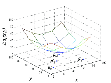
Figure 1: Illustrating the function $\mathsf{E}\mathrm{d}_{i}(x,y)$ of an uncertain point $P_{i}$ with $m=4$.

Let $X_{i}=\{x_{i1},x_{i2},\cdots,x_{im}\}$ be the set of the $x$-coordinates of all locations of $P_{i}$ sorted in ascending order. Let $Y_{i}=\{y_{i1},y_{i2},\cdots,y_{im}\}$ be the set of their $y$-coordinates in ascending order. Note that $X_{i}$ and $Y_{i}$ can be obtained in $O(m)$ time from the input (recall that the locations of $P_{i}$ are given in two sorted lists in the input). For convenience of discussion, we let $x_{i0}=-\infty$, and let $X_{i}$ also include $x_{i0}$. Similarly, let $y_{i0}=-\infty$, and let $Y_{i}$ also include $y_{i0}$. Note that due to our general position assumption, the values in $X_{i}$ (resp., $Y_{i}$) are distinct.

For any value $z$, we refer to the largest value in $X_{i}$ that is smaller or equal to $z$ the predecessor of $z$ in $X_{i}$, and we use $I_{z}(X_{i})$ to denote the index of the predecessor. Similarly, $I_{z}(Y_{i})$ is the index of the predecessor of $z$ in $Y_{i}$.

Consider any point $q$ in the plane. The predecessor of the $x$-coordinate of $q$ in $X_{i}$ is also called the predecessor of $q$ in $X_{i}$. Similarly, the predecessor of the $y$-coordinate of $q$ in $Y_{i}$ is also called the predecessor of $q$ in $Y_{i}$. We use $I_{q}(X_{i})$ and $I_{q}(Y_{i})$ to denote their indices, respectively.

Consider any cell $C$ of the grid $G_{i}$. For convenience of discussion, we assume $C$ contains its left and bottom sides, but does not contain its top and right sides. In this way, any point in the plane is contained in one and only one cell of $G_{i}$. Further, all points of $C$ have the same predecessor in $X_{i}$ and also have the same predecessor in $Y_{i}$. This allows us to define the predecessor of $C$ in $X_{i}$ as the predecessor of any point in $X_{i}$, and we use $I_{C}(X_{i})$ to denote the index of the predecessor. We define $I_{C}(Y_{i})$ similarly. We have the following lemma.

Lemma 1

For any uncertain point $P_{i}\in\mathcal{P}$, after $O(m)$ time preprocessing, for any cell $C$ of the grid $G_{i}$, if $I_{C}(X_{i})$ and $I_{C}(Y_{i})$ are known, then the function $\mathsf{E}\mathrm{d}_{i}(x,y,C)$ can be computed in constant time.

Proof

For each location $p\in P_{i}$, let $x_{p}$ and $y_{q}$ be the $x$- and $y$-coordinates of $p$, respectively, and let $f_{p}$ be the probability associated with $p$.

For any point $q=(x,y)$ in $\mathbb{R}^{2}$, recall that the expected distance function $\mathsf{E}\mathrm{d}_{i}(x,y)=\sum_{p\in P_{i}}f_{p}\cdot d(p,q)=\sum_{p\in P_{i}}f_{p}\cdot(|x_{p}-x|+|y_{p}-y|)$. Therefore, we can write $\mathsf{E}\mathrm{d}_{i}(x,y)=\sum_{p\in P_{i}}f_{p}\cdot|x_{p}-x|+\sum_{p\in P_{i}}f_{p}\cdot|y_{p}-y|$. In the following, we first discuss how to compute $\sum_{p\in P_{i}}f_{p}\cdot|x_{p}-x|$ and the case for $\sum_{p\in P_{i}}f_{p}\cdot|y_{p}-y|$ is very similar.

Let $S_{1}$ denote the set of all locations of $P_{i}$ whose $x$-coordinates are smaller than or equal to $x$, i.e., the $x$-coordinate of $q$. Let $S_{2}=P_{i}\setminus S_{1}$. Then, we have the following:

$$\begin{split}\sum_{p\in P_{i}}f_{p}\cdot|x_{p}-x|&=\sum_{p\in S_{1}}f_{p}\cdot(x-x_{p})+\sum_{p\in S_{2}}f_{p}\cdot(x_{p}-x)\\ &=x\cdot\big{(}\sum_{p\in S_{1}}f_{p}-\sum_{p\in S_{2}}f_{p}\big{)}-\sum_{p\in S_{1}}f_{p}\cdot x_{p}+\sum_{p\in S_{2}}f_{p}\cdot x_{p}\\ &=x\cdot\big{(}2\cdot\sum_{p\in S_{1}}f_{p}-\sum_{p\in P_{i}}f_{p}\big{)}-2\sum_{p\in S_{1}}f_{p}\cdot x_{p}+\sum_{p\in P_{i}}f_{p}\cdot x_{p}.\end{split}$$ (1)

Thus, in order to compute $\sum_{p\in P_{i}}f_{p}\cdot|x_{p}-x|$, it is sufficient to know the four values $\sum_{p\in S_{1}}f_{p}$, $\sum_{p\in P_{i}}f_{p}$, $\sum_{p\in S_{1}}f_{p}\cdot x_{p}$, and $\sum_{p\in P_{i}}f_{p}\cdot x_{p}$. To this end, we do the following preprocessing.

First, we compute $\sum_{p\in P_{i}}f_{p}$ and $\sum_{p\in P_{i}}f_{p}\cdot x_{p}$, which can be done in $O(m)$ time. Second, recall that $X_{i}=\{x_{i0},x_{i1},\ldots,x_{im}\}$ maintains the $x$-coordinates of the locations of $P_{i}$ sorted in ascending order. Note that given any index $j$ with $1\leq j\leq m$, we can access the information of the location of $P_{i}$ whose $x$-coordinate is $x_{ij}$ in constant time, and this can be done by linking each $x_{ij}$ to the corresponding location of $P_{i}$ when we create the list $X_{i}$ from the input. For each $j$ with $1\leq j\leq n$, we let $f(j)$ be the probability associated with the location of $P_{i}$ whose $x$-coordinate is $x_{ij}$.

In the preprocessing, we compute two arrays $A[0\cdots m]$ and $B[0\cdots m]$. Specifically, for each $1\leq j\leq n$, $A[j]=\sum_{k=1}^{j}f(k)$ and $B[j]=\sum_{k=1}^{j}f(k)\cdot x_{ik}$. For $j=0$, we let $A[0]=B[0]=0$. As discussed above, since we can access $f(j)$ in constant time for any $1\leq j\leq m$, the two arrays $A$ and $B$ can be computed in $O(m)$ time.

Let $t=I_{q}(X_{i})$, i.e., the index of the predecessor of $q$ in $X_{i}$. Note that $t\in[0,m]$. To compute $\sum_{p\in P_{i}}f_{p}\cdot|x_{p}-x|$, an easy observation is that $\sum_{p\in S_{1}}f_{p}$ is exactly equal to $A[t]$ and $\sum_{p\in S_{1}}f_{p}\cdot x_{p}$ is exactly equal to $B[t]$. Therefore, with the above preprocessing, if $t$ is known, according to Equation (1), $\sum_{p\in P_{i}}f_{p}\cdot|x_{p}-x|$ can be computed in $O(1)$ time.

The above shows that with $O(m)$ time preprocessing, given $I_{q}(X_{i})$, we can compute the function $\sum_{p\in P_{i}}f_{p}\cdot|x_{p}-x|$ of $x$ at $q=(x,y)$ in constant time.

In a similar way, with $O(m)$ time preprocessing, given $I_{q}(Y_{i})$, we can compute the function $\sum_{p\in P_{i}}f_{p}\cdot|y_{p}-y|$ of $y$ at $p=(x,y)$ in constant time.

Let $q$ be any point in the cell $C$. Hence, $I_{q}(X_{i})=I_{C}(X_{i})$ and $I_{q}(Y_{i})=I_{C}(Y_{i})$. Further, the function $\mathsf{E}\mathrm{d}_{i}(x,y)$ on $q=(x,y)\in C$ is exactly the function $\mathsf{E}\mathrm{d}_{i}(x,y,C)$. Therefore, with $O(m)$ time preprocessing, given $I_{C}(X_{i})$ and $I_{C}(Y_{i})$, we can compute the function $\mathsf{E}\mathrm{d}_{i}(x,y,C)$ in constant time.

The lemma thus follows. ∎

Due to Lemma 1, we have the following corollary.

Corollary 1

For each uncertain point $P_{i}\in\mathcal{P}$, after $O(m)$ time preprocessing, given any point $q$ in the plane, the expected distance $\mathsf{E}\mathrm{d}(P_{i},q)$ can be computed in $O(\log m)$ time.

Proof

Given any point $q\in\mathbb{R}^{2}$, we can compute $I_{q}(X_{i})$ in $O(\log m)$ time by doing binary search on $X_{i}$. Similarly, we can compute $I_{q}(Y_{i})$ in $O(\log m)$ time. Let $C$ be the cell containing $q$. Recall that $I_{C}(X_{i})=I_{q}(X_{i})$ and $I_{C}(Y_{i})=I_{q}(Y_{i})$. Hence, by Lemma 1, we can compute the function $\mathsf{E}\mathrm{d}_{i}(x,y,C)$ in constant time. Then, $\mathsf{E}\mathrm{d}(P_{i},q)$ is equal to $\mathsf{E}\mathrm{d}_{i}(q_{x},q_{y},C)$, where $q_{x}$ and $q_{y}$ are the $x$- and $y$-coordinates of $q$, respectively. Thus, after $\mathsf{E}\mathrm{d}_{i}(x,y,C)$ is known, $\mathsf{E}\mathrm{d}(P_{i},q)$ can be computed in constant time. The corollary thus follows. ∎

Recall that $\mathsf{E}\mathrm{d}_{\max}(q)=\max_{P_{i}\in\mathcal{P}}\mathsf{E}\mathrm{d}(P_{i},q)$ for any point $q$ in the plane. For convenience, we use $\mathsf{E}\mathrm{d}_{\max}(x,y)$ to represent $\mathsf{E}\mathrm{d}_{\max}(q)$ as a function of $q=(x,y)\in\mathbb{R}^{2}$. Note that $\mathsf{E}\mathrm{d}_{\max}(x,y)$ is the upper envelope of the functions $\mathsf{E}\mathrm{d}_{i}(x,y)$ for all $i=1,2,\ldots,n$. Since each $\mathsf{E}\mathrm{d}_{i}(x,y)$ is convex on $\mathbb{R}^{2}$, $\mathsf{E}\mathrm{d}_{\max}(x,y)$ is also convex on $\mathbb{R}^{2}$. Further, the rectilinear center $q^{*}$ corresponds to a lowest point $p^{*}$ on $\mathsf{E}\mathrm{d}_{\max}(x,y)$. Specifically, $q^{*}$ is the projection of $p^{*}$ on the $xy$-plane. Therefore, computing $q^{*}$ is equivalent to computing a lowest point in the upper envelope of all functions $\mathsf{E}\mathrm{d}_{i}(x,y)$ for all $i=1,2,\ldots,n$.

For each $1\leq i\leq n$, let $H_{i}$ denote the set of supporting planes of all surface patches of the function $\mathsf{E}\mathrm{d}_{i}(x,y)$. Let $\mathcal{H}=\cup_{i=1}^{n}H_{i}$. Since $\mathsf{E}\mathrm{d}_{i}(x,y)$ is convex, $\mathsf{E}\mathrm{d}_{i}(x,y)$ is essentially the upper envelope of the planes in $H_{i}$. Hence, $\mathsf{E}\mathrm{d}_{max}(x,y)$ is also the upper envelope of all planes in $\mathcal{H}$. Therefore, as discussed in Section 1.2, finding $p^{*}$ is essentially a 3D LP problem on $\mathcal{H}$, which can be solved in $O(|\mathcal{H}|)$ time by Megiddo’s technique [15]. Since the size of each $H_{i}$ is $\Theta(m^{2})$, $|\mathcal{H}|=\Theta(nm^{2})$. Therefore, applying the algorithm in [15] directly can solve the problem in $O(nm^{2})$ time. In the following, we give an $O(nm)$ time algorithm.

In the following paper, we assume we have done the preprocessing of Lemma 1 for each $P_{i}\in\mathcal{P}$, which takes $O(mn)$ time in total.

3 The Decision Algorithm

In this section, we present a decision algorithm that solves a decision problem, which is needed later in Section 4. We first introduce the decision problem.

Let $R=[x_{1},x_{2};y_{1},y_{2}]$ be an axis-parallel rectangle in the plane, where $x_{1}$ and $x_{2}$ are the $x$-coordinates of the left and right sides of $R$, respectively, and $y_{1}$ and $y_{2}$ are the $y$-coordinates of the bottom and top sides of $R$, respectively. Suppose it is known that $q^{*}$ is in $R$ (but the exact location of $q^{*}$ is not known). Let $L$ be an arbitrary line that intersects the interior of $R$. The decision problem asks whether $q^{*}$ is on $L$, and if not, which side of $L$ contains $q^{*}$. We assume the two predecessor indices $I_{x_{1}}(X_{i})$ and $I_{y_{1}}(Y_{i})$ are already known.

For each $1\leq i\leq n$, let $a_{i}=I_{x_{2}}(X_{i})-I_{x_{1}}(X_{i})+1$ and $b_{i}=I_{y_{2}}(Y_{i})-I_{y_{1}}(Y_{i})+1$. In fact, $a_{i}$ and $b_{i}$ are the numbers of columns and rows of $G_{i}$ that intersect $R$, respectively. Below, we give a decision algorithm that solves the decision problem in $O(\sum_{i=1}^{n}(a_{i}+b_{i}))$ time. Note that $2n\leq\sum_{i=1}^{n}(a_{i}+b_{i})\leq 2(m+1)n$.

We first show that the decision problem can be solved in $O(\sum_{i=1}^{n}a_{i}\cdot b_{i})$ time by using the decision algorithm for the 3D LP problem [15]. Later we will reduce the running time to $O(\sum_{i=1}^{n}(a_{i}+b_{i}))$ time.

Recall that $p^{*}$ is a lowest point in the upper envelope of the functions $\mathsf{E}\mathrm{d}_{i}(x,y)$ for $i=1,2,\ldots,n$. Since $q^{*}$ is in $R$ and each function $\mathsf{E}\mathrm{d}_{i}(x,y)$ is convex, an easy observation is that $p^{*}$ is also a lowest point in the upper envelope of $\mathsf{E}\mathrm{d}_{i}(x,y)$ for $i=1,2,\ldots,n$ restricted on $(x,y)\in R$. This implies that we only need to consider each function $\mathsf{E}\mathrm{d}_{i}(x,y)$ restricted on $R$.

For each $1\leq i\leq n$, let $G_{i}(R)$ be the set of cells of $G_{i}$ that intersect $R$, and let $H_{i}(R)$ be the set of supporting planes of the surface patches of $\mathsf{E}\mathrm{d}(P_{i},q)$ defined on the cells of $G_{i}(R)$. Let $\mathcal{H}(R)=\cup_{i=1}^{n}H_{i}(R)$. By our above analysis, $p^{*}$ is a lowest point of the upper envelope of all planes in $\mathcal{H}(R)$. Note that $|H_{i}(R)|=a_{i}\cdot b_{i}$ for each $1\leq i\leq n$. Thus, $|\mathcal{H}(R)|=\sum_{i=1}^{n}a_{i}\cdot b_{i}$. Then, we can apply the decision algorithm in [15] (Section 5.2) on $\mathcal{H}(R)$ to determine which side of $L$ contains $q^{*}$ in $O(|\mathcal{H}(R)|)$ time. In order to explain our improved algorithm later, we sketch this algorithm below.

We consider each plane of $\mathcal{H}(R)$ as a function of the points $q$ on the $xy$-plane $\mathbb{R}^{2}$. In the first step, the algorithm finds a point $q^{\prime}$ on $L$ that minimizes the maximum value of all functions in $\mathcal{H}(R)$ restricted on the line $q\in L$. This is essentially a 2D LP problem because each function of $\mathcal{H}(R)$ restricted on $L$ is a line, and thus the problem can be solved in $O(|\mathcal{H}(R)|)$ time [15]. Let $\Phi_{q^{\prime}}$ be the set of functions of $\mathcal{H}(R)$ whose values at $q^{\prime}$ are equal to the above maximum value. The set $\Phi_{q^{\prime}}$ can be found in $O(|\mathcal{H}(R)|)$ time after $q^{\prime}$ is computed. This finishes the first step, which takes $O(|\mathcal{H}(R)|)=O(\sum_{i=1}^{n}a_{i}\cdot b_{i})$ time.

The second step solves another two instances of the 2D LP problem on the planes of $\Phi_{q^{\prime}}$, which takes $O(|\Phi_{q^{\prime}}|)$ time. An easy upper bound for $|\Phi_{q^{\prime}}|$ is $\sum_{i=1}^{n}a_{i}\cdot b_{i}$. A close analysis can show that $|\Phi_{q^{\prime}}|=O(n)$. Indeed, for each $1\leq i\leq n$, since the function $\mathsf{E}\mathrm{d}_{i}(x,y)$ is convex, among all $a_{i}\cdot b_{i}$ planes in $H_{i}(R)$, at most four of them are in $\Phi_{q^{\prime}}$. Therefore, $|\Phi_{q^{\prime}}|=O(n)$. Hence, the second step runs in $O(n)$ time. Since in our problem there always exists a solution, according to [15], the second step will either conclude that $q^{\prime}$ is $q^{*}$ or tell which side of $L$ contains $q^{*}$, which solves the decision problem. The algorithm takes $O(\sum_{i=1}^{n}a_{i}\cdot b_{i})$ time in total, which is dominated by the first step.

In the sequel, we reduce the running time of the above algorithm, in particular, the first step, to $O(\sum_{i=1}^{n}(a_{i}+b_{i}))$. Our goal is to compute $q^{\prime}$ and $\Phi_{q^{\prime}}$. By the definition, $q^{\prime}$ is a lowest point in the upper envelope of all functions of $\mathcal{H}(R)$ restricted on the line $L$. Consider any uncertain point $P_{i}\in\mathcal{P}$. Let $H_{i}(R,L)$ be the set of supporting planes of the surface patches defined on the cells of $G_{i}(R)$ intersecting $L$. Observe that since $\mathsf{E}\mathrm{d}_{i}(x,y)$ is convex, the upper envelope of all the functions of $H_{i}(R)$ restricted on $L$ is exactly the upper envelope of the functions of $H_{i}(R,L)$ restricted on $L$. Therefore, $q^{\prime}$ is also a lowest point in the upper envelope of the functions of $\mathcal{H}(R,L)$ restricted on $L$, where $\mathcal{H}(R,L)=\cup_{i=1}^{n}H_{i}(R,L)$. In other words, among all planes in $\mathcal{H}(R)$, only the planes of $\mathcal{H}(R,L)$ are relevant for determining $q^{\prime}$. Thus, suppose $\mathcal{H}(R,L)$ has been computed; then $q^{\prime}$ can be computed based on the planes of $\mathcal{H}(R,L)$ in $O(|\mathcal{H}(R,L)|)$ time by the 2D LP algorithm [15]. After $q^{\prime}$ is computed, the set $\Phi_{q^{\prime}}$ can also be determined in $O(|\mathcal{H}(R,L)|)$ time.

Note that $|\mathcal{H}(R,L)|=O(\sum_{i=1}^{n}(a_{i}+b_{i}))$, since for each $1\leq i\leq n$, $|H_{i}(R,L)|$, which is equal to the number of cells of $G_{i}(R)$ intersecting $L$, is $O(a_{i}+b_{i})$.

It remains to compute $\mathcal{H}(R,L)$, i.e., compute $H_{i}(R,L)$ for each $1\leq i\leq n$. Recall that $R=[x_{1},x_{2};y_{1},y_{2}]$ and the two predecessor indices $I_{x_{1}}(X_{i})$ and $I_{y_{1}}(Y_{i})$ for each $1\leq i\leq n$ are already known. The following lemma gives an $O(a_{i}+b_{i})$ algorithm to compute $H_{i}(R,L)$.

Lemma 2

For each $1\leq i\leq n$, $H_{i}(R,L)$ can be computed in $O(a_{i}+b_{i})$ time.

Proof

Let $G_{i}(R,L)$ be the set of cells of $G_{i}(R)$ intersecting $L$. To compute the planes in $H_{i}(R,L)$, it is sufficient to determine the plane surface patches of $\mathsf{E}\mathrm{d}_{i}(x,y)$ defined on the cells of $G_{i}(R,L)$. By Lemma 1, this amounts to determine the indices of the predecessors of these cells in $X_{i}$ and $Y_{i}$, respectively. In the following, we give an algorithm to compute the cells of $G_{i}(R,L)$ and determine their predecessor indices in $X_{i}$ and $Y_{i}$, respectively, and the algorithm runs in $O(a_{i}+b_{i})$ time.

The main idea is that we first pick a particular point $p$ on $L\cap R$ and locate the cell of $G_{i}(R)$ containing $p$ (clearly this cell belongs to $G_{i}(R,L)$), and then starting from $p$, we traverse on $L$ and $G_{i}(R)$ simultaneously to trace other cells of $G_{i}(R,L)$ until we move out of $R$. The details are given below.

We focus on the case where $L$ has a positive slope. The other cases can be handled similarly. Recall that $L$ intersects the interior of $R$. Let $p$ be the leftmost intersection of $L$ with the boundary of $R$. Hence, $p$ is either on the left side or the bottom side of $R$.

Let $C$ be the cell of $G_{i}$ that contains $p$. We first determine the two indices $I_{p}(X_{i})$ and $I_{p}(Y_{i})$. Note that $I_{C}(X_{i})=I_{p}(X_{i})$ and $I_{C}(Y_{i})=I_{p}(Y_{i})$.

Since $p\in R$, the index $I_{p}(X_{i})$ can be found in $O(a_{i})$ time by scanning the list $X_{i}$ from the index $I_{x_{1}}(X_{i})$. Similarly, $I_{p}(Y_{i})$ can be found in $O(b_{i})$ time by scanning the list $Y_{i}$ from the index $I_{y_{1}}(Y_{i})$. After $I_{C}(X_{i})=I_{p}(X_{i})$ and $I_{C}(Y_{i})=I_{p}(Y_{i})$ are computed, by Lemma 1, the function $\mathsf{E}\mathrm{d}_{i}(x,y,C)$ can be computed in constant time, and we add the function to $H_{i}(R,L)$.

Next, we move $p$ on $L$ rightwards. We will show that when $p$ crosses the boundary of $C$, we can determine the new cell containing $p$ and update the two indices $I_{p}(X_{i})$ and $I_{p}(Y_{i})$ in constant time. This process continues until $p$ moves out of $R$. Specifically, when $p$ moves on $L$ rightwards, $p$ will cross the boundary of $C$ either from the top side or the right side.

First, we determine whether $p$ will move out of $R$ before $p$ crosses the boundary of $C$. If yes, then we terminate the algorithm. Otherwise, we determine whether $p$ moves out of $C$ from its right side or left side. All above can be easily done in constant time. Depending on whether $p$ crosses the boundary of $C$ from its top side, right side, or from both sides simultaneously, there are three cases.

1. If $p$ crosses the boundary of $C$ from the top side and $p$ does not cross the right side of $C$, then $p$ enters into a new cell that is on top of $C$. We update $C$ to the new cell. We increase the index $I_{p}(Y_{i})$ by one, but keep $I_{p}(X_{i})$ unchanged. Clearly, the above two indices are correctly updated and $I_{C}(X_{i})=I_{p}(X_{i})$ and $I_{C}(Y_{i})=I_{p}(Y_{i})$ for the new cell $C$. Again, by Lemma 1, the function $\mathsf{E}\mathrm{d}_{i}(x,y,C)$ for the new cell $C$ can be computed in constant time. We add the new function to $H_{i}(R,L)$.

2. If $p$ crosses the boundary of $C$ from the right side and $p$ does not cross the top side of $C$, then $p$ enters into a new cell that is on right of $C$. The algorithm in this case is similar to the above case and we omit the discussions.

3. The remaining case is when $p$ crosses the boundary of $C$ through the top right corner of $C$. In this case, $p$ enters into the northeast neighboring cell of $C$. We first add to $H_{i}(R,L)$ the supporting planes of the surface patches of $\mathsf{E}\mathrm{d}_{i}(x,y)$ defined on the top neighboring cell and the right neighboring cell of $C$, which can be computed in constant time as the above two cases. Then, we update $C$ to the new cell $p$ is entering. We increase each of $I_{p}(X_{i})$ and $I_{p}(Y_{i})$ by one. Again, the two indices are correctly updated for the new cell $C$. Finally, we compute the new function $\mathsf{E}\mathrm{d}_{i}(x,y,C)$ and add it to $H_{i}(R,L)$.

When the algorithm stops, $H_{i}(R,L)$ is computed. In general, during the procedure of moving $p$ on $L$, we spend constant time on finding each supporting plane of $H_{i}(R,L)$. Therefore, the total running time of the entire algorithm is $O(a_{i}+b_{i})$. The lemma thus follows. ∎

With the preceding lemma, we have the following result.

Theorem 3.1

The decision problem can be solved in $O(\sum_{i=1}^{n}(a_{i}+b_{i}))$ time.

4 Computing the Rectilinear Center

In this section, with the help of our decision algorithm in Section 3, we compute the rectilinear center $q^{*}$ in $O(mn)$ time.

As discussed in Section 1.2, our algorithm is a prune-and-search algorithm that has $O(\log n)$ “outer” recursive steps each of which has $O(\log m)$ “inner” recursive steps. In each outer recursive step, the algorithm prunes at least $|\mathcal{P}|/32$ uncertain points of $\mathcal{P}$ such that these uncertain points are not relevant for computing $q^{*}$. After $O(\log n)$ outer recursive steps, there will be only a constant number of uncertain points remaining in $\mathcal{P}$. Each outer recursive step runs in $O(m|\mathcal{P}|)$ time, where $|\mathcal{P}|$ is the number of uncertain points remaining in $\mathcal{P}$. In this way, the total running time of the algorithm is $O(mn)$.

Each outer recursive step is another recursive prune-and-search algorithm, which consists of $2+\log m$ inner recursive steps. Let $\mathcal{X}=\cup_{i=1}^{n}X_{i}$ and $\mathcal{Y}=\cup_{i=1}^{n}Y_{i}$. Hence, $|\mathcal{X}|=|\mathcal{Y}|=mn$. We maintain a rectangle $R=[x_{1},x_{2};y_{1},y_{2}]$ that contains $q^{*}$. Initially, $R$ is the entire plane. In each inner recursive step, we shrink $R$ such that the $x$-range $[x_{1},x_{2}]$ (resp., $y$-range $[y_{1},y_{2}]$) of the new $R$ only contains half of the values of $\mathcal{X}$ (resp., $\mathcal{Y}$) in the $x$-range (resp., $y$-range) of the previous $R$. In this way, after $\log m+2$ inner recursive steps, the $x$-range (resp., $y$-range) of $R$ only contains at most $n/4$ values of $\mathcal{X}$ (resp., $\mathcal{Y}$). At this moment, a key observation is that there is a subset $\mathcal{P}^{*}$ of at least $n/2$ uncertain points, such that for each $P_{i}\in\mathcal{P}^{*}$, $R$ is contained in the interior of a cell of the grid $G_{i}$, i.e., the $x$-range (resp., $y$-range) of $R$ does not contain any value of $X_{i}$ (resp., $Y_{i}$). Due to the observation, we can use a pruning procedure similar to that in [15] to prune at least $|\mathcal{P}^{*}|/16\geq n/32$ uncertain points.

In the following, in Section 4.1, we give our algorithm on pruning the values of $\mathcal{X}$ and $\mathcal{Y}$ to obtain $\mathcal{P}^{*}$. In Section 4.2, we prune uncertain points of $\mathcal{P}^{*}$.

4.1 Pruning the Coordinate Values of $\mathcal{X}$ and $\mathcal{Y}$

Consider a general step of the algorithm where we are about to perform the $j$-th inner recursive step for $1\leq j\leq\log m+2$. Our algorithm maintains the following algorithm invariants. (1) We have a rectangle $R^{j-1}=[x_{1}^{j-1},x_{2}^{j-1};y_{1}^{j-1},y_{2}^{j-1}]$ that contains $q^{*}$. (2) For each $1\leq i\leq n$, the index $I_{x_{1}^{j-1}}(X_{i})$ of the predecessor of $x_{1}^{j-1}$ in $X_{i}$ is known, and so is the index $I_{y_{1}^{j-1}}(Y_{i})$. (3) We have a sublist $X_{i}^{j-1}$ of $X_{i}$ that consists of all values of $X_{i}$ in $[x_{1}^{j-1},x_{2}^{j-1}]$ and a sublist $Y_{i}^{j-1}$ of $Y_{i}$ that consists of all values of $Y_{i}$ in $[y_{1}^{j-1},y_{2}^{j-1}]$. Note that these sublists can be empty. (4) $|\mathcal{X}^{j-1}|\leq mn/2^{j-1}$ and $|\mathcal{Y}^{j-1}|\leq mn/2^{j-1}$, where $\mathcal{X}^{j-1}=\cup_{i=1}^{n}X_{i}^{j-1}$ and $\mathcal{Y}^{j-1}=\cup_{i=1}^{n}Y_{i}^{j-1}$.

Initially, we set $R^{0}=[-\infty,+\infty;-\infty,+\infty]$, $X_{i}^{0}=X_{i}$ and $Y_{i}^{0}=Y_{i}$ for each $1\leq i\leq n$, with $\mathcal{X}^{0}=\mathcal{X}$ and $\mathcal{Y}^{0}=\mathcal{Y}$. It is easy to see that before we start the first inner recursive step for $j=1$, all the algorithm invariants hold.

In the sequel, we give the details of the $j$-th inner recursive step. We will show that its running time is $O(mn/2^{j}+n)$ and all algorithm invariants are still maintained after the step.

Let $x_{m}$ be the median of $\mathcal{X}^{j-1}$ and $y_{m}$ be the median of $\mathcal{Y}^{j-1}$. Both $x_{m}$ and $y_{m}$ can be found in $O(|\mathcal{X}^{j-1}|+|\mathcal{Y}^{j-1}|)$ time.

For each $1\leq i\leq n$, let $a_{i}^{j-1}=I(x_{2}^{j-1})-I(x_{1}^{j-1})+1$ and $b_{i}^{j-1}=I(y_{2}^{j-1})-I(y_{1}^{j-1})+1$. Observe that $a_{i}^{j-1}=|X_{i}^{j-1}|+1$ and $b_{i}^{j-1}=|Y_{i}^{j-1}|+1$.

Let $x^{*}$ and $y^{*}$ be the $x$- and $y$-coordinates of $q^{*}$, respectively.

We first determine whether $x^{*}>x_{m}$, $x^{*}<x_{m}$, or $x^{*}=x_{m}$. This can be done by applying our decision algorithm on $R^{j-1}$ and $L$ with $L$ being the vertical line $x=x_{m}$. By Theorem 3.1, the running time of our decision algorithm is $O(\sum_{i=1}^{n}(a_{i}^{j-1}+b_{i}^{j-1}))$, which is $O(n+|\mathcal{X}^{j-1}|+|\mathcal{Y}^{j-1}|)$.

Note that if $x^{*}=x_{m}$, then according to our decision algorithm, $q^{*}$ will be found by the decision algorithm and we can terminate the entire algorithm. Otherwise, without loss of generality, we assume $x^{*}>x_{m}$. We proceed to determine whether $y^{*}>y_{m}$ or $y^{*}<y_{m}$, or $y^{*}=y_{m}$ by applying our decision algorithm on $R^{j-1}$ and $L$ with $L$ being the horizontal line $y=y_{m}$. Similarly, if $y^{*}=y_{m}$, then the decision algorithm will find $q^{*}$ and we are done. Otherwise, without loss of generality we assume $y^{*}>y_{m}$. The above calls our decision algorithm twice, which takes $O(n+|\mathcal{X}^{j-1}|+|\mathcal{Y}^{j-1}|)$ time in total.

Now we know that $q^{*}$ is in the rectangle $[x_{m},x_{2}^{j-1};y_{m},y_{2}^{j-1}]$. We let $R^{j}=[x_{1}^{j},x_{2}^{j};y_{1}^{j},y_{2}^{j}]$ be the above rectangle, i.e., $x_{1}^{j}=x_{m}$, $x_{2}^{j}=x_{2}^{j-1}$, $y_{1}^{j}=y_{m}$, and $y_{2}^{j}=y_{2}^{j-1}$. Clearly, the first algorithm invariant is maintained.

We further proceed as follows to maintain the other three invariants.

For each $1\leq i\leq n$, by scanning the sorted list $X_{i}^{j-1}$, we compute the index $I_{x_{1}^{j}}(X_{i})$ of the predecessor of $x_{1}^{j}$ in $X_{i}$ (each element of $X_{i}^{j-1}$ maintains its original index in $X_{i}$), and similarly, by scanning the sorted list $Y^{j-1}_{i}$, we compute the index $I_{y_{1}^{j}}(Y_{i})$. Computing these indices in all $X_{i}$ and $Y_{i}$ for $i=1,2,\ldots,n$ can be done in $O(|\mathcal{X}^{j-1}|+|\mathcal{Y}^{j-1}|)$ time. This maintains the second algorithm invariant.

Next, for each $1\leq i\leq n$, we scan $X_{i}^{j-1}$ to compute a sublist $X_{i}^{j}$, which consists of all values of $X_{i}^{j-1}$ in $[x_{1}^{j},x_{2}^{j}]$, and similarly, we scan $Y_{i}^{j-1}$ to compute a sublist $Y_{i}^{j}$, which consists of all values of $Y_{i}^{j-1}$ in $[y_{1}^{j},y_{2}^{j}]$. Computing the lists $X_{i}^{j}$ and $Y_{i}^{j}$ for all $i=1,2,\ldots,n$ as above can be done in overall $O(|\mathcal{X}^{j-1}|+|\mathcal{Y}^{j-1}|)$ time. This maintains the third algorithm invariant.

Let $\mathcal{X}^{j}=\sum_{i=1}^{n}X_{i}^{j}$ and $\mathcal{Y}^{j}=\sum_{i=1}^{n}Y_{i}^{j}$. According to our above algorithm, $|\mathcal{X}^{j}|\leq|\mathcal{X}^{j-1}|/2$ and $|\mathcal{Y}^{j}|\leq|\mathcal{Y}^{j-1}|/2$. Since $|\mathcal{X}^{j-1}|\leq nm/2^{j-1}$ and $|\mathcal{Y}^{j-1}|\leq nm/2^{j-1}$, we obtain $|\mathcal{X}^{j}|\leq nm/2^{j}$ and $|\mathcal{Y}^{j}|\leq nm/2^{j}$. Hence, the fourth algorithm invariant is maintained.

In summary, after the $j$-th inner recursive step, all four algorithm invariants are maintained. Our above analysis also shows that the total running time is $O(n+|\mathcal{X}^{j-1}|+|\mathcal{Y}^{j-1}|)$, which is $O(nm/2^{j}+n)$.

We stop the algorithm after the $t$-th inner recursive step, for $t=2+\log m$. The total time for all $t$ steps is thus $O(\sum_{j=1}^{t}(n+mn/2^{j}))=O(mn)$.

After the $t$-th step, by our algorithm invariants, the rectangle $R^{t}$ contains $q^{*}$, and $|\mathcal{X}^{t}|\leq mn/2^{t}=n/4$ and $|\mathcal{Y}^{t}|\leq mn/2^{t}=n/4$.

We say that an uncertain point $P_{i}$ is prunable if both $X_{i}^{t}$ and $Y_{i}^{t}$ are empty (and thus $R^{t}$ is contained in the interior of a cell of $G_{i}$). Let $\mathcal{P}^{*}$ denote the set of all prunable uncertain points of $\mathcal{P}$. The following is an easy but crucial observation.

Observation 2

$|\mathcal{P}^{*}|\geq n/2$.

Proof

Since $\mathcal{X}^{t}\leq n/4$, among the $n$ sets $X_{i}^{t}$ for $i=1,2,\ldots,n$, at most $n/4$ of them are non-empty. Similarly, since $\mathcal{Y}^{t}\leq n/4$, among the $n$ sets $Y_{i}^{t}$ for $i=1,2,\ldots,n$, at most $n/4$ of them are non-empty. Therefore, there are at most $n/2$ uncertain points $P_{i}\in\mathcal{P}$ such that either $X_{i}^{t}$ or $Y_{i}^{t}$ is non-empty. This implies that there are at least $n/2$ prunable uncertain points in $\mathcal{P}$. ∎

After the $t$-th inner recursive step, the set $\mathcal{P}^{*}$ can be obtained in $O(n)$ time by checking all sets $X_{i}^{t}$ and $Y_{i}^{t}$ for $i=1,2,\ldots,n$ and see whether they are empty.

The reason we are interested in prunable uncertain points is that for each prunable uncertain point $P_{i}$ of $\mathcal{P}^{*}$, since $R^{t}$ contains $q^{*}$ and $R_{t}$ is contained in a cell $C_{i}$ of $G_{i}$, there is only one surface patch of $\mathsf{E}\mathrm{d}_{i}(x,y)$ (i.e., the one defined on $C_{i}$) that is relevant for computing $q^{*}$. Let $h_{i}$ denote the supporting plane of the above surface patch. We call $h_{i}$ the relevant plane of $P_{i}$. Note that we can obtain $h_{i}$ in constant time. Indeed, observe that the predecessor index $I_{C_{i}}(X_{i})$ is exactly $I_{x_{1}^{t}}(X_{i})$, which is known by our algorithm invariants. Similarly, the index $I_{C_{i}}(Y_{i})$ is also known. By Lemma 1, the function $\mathsf{E}\mathrm{d}_{i}(x,y,C_{i})$, which is also the function of $h_{i}$, can be obtained in constant time. Hence, the relevant planes of all prunable uncertain points of $\mathcal{P}^{*}$ can be obtained in $O(n)$ time.

Remark.

One may wonder why we did not perform the inner recursive steps for $t=\log mn$ times (instead of $t=2+\log m$ time) so that $\mathcal{X}^{t}$ and $\mathcal{Y}^{t}$ would each have a constant number of values in the range of $R$. The reason is that based on our analysis, that would take $O(mn+n\log nm)$ time, which may not be bounded by $O(mn)$ (e.g., when $m=o(\log n)$). In fact, performing the inner recursive steps for $t=2+\log m$ times such that $\mathcal{X}^{t}$ and $\mathcal{Y}^{t}$ each have at most $\frac{n}{4}$ values in the range of $R$ is an interesting and crucial ingredient of our techniques.

4.2 Pruning Uncertain Points from $\mathcal{P}^{*}$

Consider a prunable uncertain point $P_{i}$ of $\mathcal{P}^{*}$. Recall that $H_{i}$ is the set of supporting planes of all surface patches of $\mathsf{E}\mathrm{d}_{i}(x,y)$. The above analysis shows that among all planes in $H_{i}$, only the relevant plane $h_{i}$ is useful for determining $q^{*}$. In other words, the point $p^{*}$, as a lowest point of all planes in $\mathcal{H}=\cup_{i=1}^{n}H_{i}$, is also a lowest point of the planes in the union of $\cup_{P_{i}\in\mathcal{P}^{*}}h_{i}$ and $\cup_{P_{i}\in\mathcal{P}\setminus\mathcal{P}^{*}}H_{i}$. This will allow us to prune at least $|\mathcal{P}^{*}|/16$ uncertain points from $\mathcal{P}^{*}$. The idea is similar to Megiddo’s pruning scheme for the 3D LP algorithm in [15].

For each $P_{i}\in\mathcal{P}^{*}$, its relevant plane $h_{i}$ is also considered as a function in the $xy$-plane. Arrange all uncertain points of $\mathcal{P}^{*}$ into $|\mathcal{P}^{*}|/2$ disjoint pairs. Let $D(\mathcal{P}^{*})$ denote the set of all these pairs. For each pair $(P_{i},P_{j})\in D(\mathcal{P}^{*})$, if the value of the function $h_{i}$ at any point of $R^{t}$ is greater than or equal to that of $h_{j}$, then $P_{j}$ can be pruned immediately; otherwise, we project the intersection of $h_{i}$ and $h_{j}$ on the $xy$-plane to obtain a line $L_{ij}$ dividing $R^{t}$ into two parts, such that $h_{i}\geq h_{j}$ on one part and $h_{i}\leq h_{j}$ on the other.

Let $\mathcal{L}$ denote the set of the dividing lines $L_{ij}$ for all pairs of $D(\mathcal{P}^{*})$. Let $L_{m}$ be the line whose slope has the median value among the lines of $\mathcal{L}$. We transform the coordinate system by rotating the $x$-axis to be parallel to $L_{m}$ (the $y$-axis does not change). For ease of discussion, we assume no other lines of $\mathcal{L}$ are parallel to $L_{m}$ (the assumption can be easily lifted; see [15]). In the new coordinate system, half the lines of $\mathcal{L}$ have negative slopes and the other half have positive slopes. We now arrange all lines of $\mathcal{L}$ into disjoint pairs such that each pair has a line of a negative slope and a line of positive slope. Let $D(\mathcal{L})$ denote the set of all these line pairs.

For each pair $(L_{i},L_{j})\in D(\mathcal{L})$, we define $y_{ij}$ as the $y$-coordinate of the intersection of $L_{i}$ and $L_{j}$. We find the median $y_{m}$ of the values $y_{ij}$ for all pairs in $D(\mathcal{L})$. Let $x^{*}$ and $y^{*}$ respectively be the $x$- and $y$-coordinate of $q^{*}$ in the new coordinate system. We determine in $O(mn)$ time whether $y^{*}>y_{m}$, $y^{*}<y_{m}$ or $y^{*}=y_{m}$ by using our decision algorithm (here an $O(mn)$ time decision algorithm is sufficient for our purpose). If $y^{*}=y_{m}$, then our decision algorithm will find $q^{*}$ and we can terminate the algorithm. Otherwise, without of loss generality, we assume $y^{*}<y_{m}$.

Let $D^{\prime}(\mathcal{L})$ denote the set of all pairs $(L_{i},L_{j})$ of $D(\mathcal{L})$ such that $y_{ij}\geq y_{m}$. Note that $|D^{\prime}(\mathcal{L})|\geq|D(\mathcal{L})|/2$. For each pair $(L_{i},L_{j})\in D^{\prime}(\mathcal{L})$, let $x_{ij}$ be the $x$-coordinate of the intersection of $L_{i}$ and $L_{j}$. We find the median $x_{m}$ of all such $x_{ij}$’s. By using our decision algorithm, we can determine in $O(mn)$ time whether $x^{*}>x_{m}$, $x^{*}<x_{m}$, or $x^{*}=x_{m}$. If $x^{*}=x_{m}$, our decision algorithm will find $q^{*}$ and we are done. Otherwise, without loss of generality, we assume $x^{*}<x_{m}$.

Figure 2: The intersection of $L_{i}$ and $L_{j}$ is in the first quarter of the intersection of $x=x_{m}$ and $y=y_{m}$ while $q^{*}$ is in the interior of the third quarter.

Now for each pair $(L_{i},L_{j})$ of $D^{\prime}(\mathcal{L})$ with $x_{ij}\geq x_{m}$ and $y_{ij}\geq y_{m}$ (there are at least $|D^{\prime}(\mathcal{L})|/2$ such pairs), we can prune either $P_{i}$ or $P_{j}$, as follows. Indeed, one of the lines in such a pair $(L_{i},L_{j})$, say $L_{i}$, has a negative slope and does not intersect the region $R=\{(x,y)\ |\ x<x_{m},\ y<y_{m}\}$ (e.g., see Fig. 2). Suppose $L_{i}$ is the dividing line of two relevant planes $h_{k_{1}}$ and $h_{k_{2}}$ of two uncertain points $P_{k_{1}}$ and $P_{k_{2}}$ of $\mathcal{P}^{*}$. It follows that either $h_{k_{1}}\geq h_{k_{2}}$ or $h_{k_{1}}\leq h_{k_{2}}$ holds on the region $R$. Since $q^{*}\in R$, one of $P_{k_{1}}$ and $P_{k_{2}}$ can be pruned.

As a summary, the above pruning algorithm prunes at least $|\mathcal{P}^{*}|/16\geq n/32$ uncertain points and the total time is $O(mn)$.

4.3 Wrapping Things Up

The algorithm in the above two subsections either computes $q^{*}$ or prunes at least $n/32$ uncertain points from $\mathcal{P}$ in $O(mn)$ time. We assume the latter case happens. Then we apply the same algorithm recursively on the remaining uncertain points for $O(\log n)$ steps, after which only a constant number of uncertain points remain. The total running time can be described by the following recurrence: $T(m,n)=T(m,\frac{31\cdot n}{32})+O(mn)$. Solving the recurrence gives $T(m,n)=O(mn)$.

Let $\mathcal{P}^{\prime}$ be the set of the remaining uncertain points, with $|\mathcal{P}^{\prime}|=O(1)$. Hence, the rectilinear center $q^{*}$ is determined by $\mathcal{P}^{\prime}$. In other words, $q^{*}$ is also a rectilinear center of $\mathcal{P}^{\prime}$. In fact, like other standard prune-and-search algorithms, the way we prune uncertain points of $\mathcal{P}$ guarantees that any rectilinear center of $\mathcal{P}$ is also a rectilinear center of $\mathcal{P}^{\prime}$, and vice versa. By using an approach similar to that in Section 4.1, Lemma 3 finally computes $q^{*}$ based on $\mathcal{P}^{\prime}$ in $O(m)$ time.

Lemma 3

The rectilinear center $q^{*}$ can be computed in $O(m)$ time.

Proof

Let $c=|\mathcal{P}^{\prime}|$, which is a constant. Let $\mathcal{X}^{\prime}=\cup_{P_{i}\in\mathcal{P}^{\prime}}X_{i}$ and $\mathcal{Y}^{\prime}=\cup_{P_{i}\in\mathcal{P}^{\prime}}Y_{i}$. We apply the same recursive algorithm in Section 4.1 on $\mathcal{X}^{\prime}$ and $\mathcal{Y}^{\prime}$ for $O(\log m)$ steps, after which we will obtain a rectangle $R$ such that $R$ contains $q^{*}$ and for each $P_{i}\in\mathcal{P}^{\prime}$, the $x$-range (resp., $y$-range) of $R$ only contains a constant number of values of $X_{i}$ (resp., $Y_{i}$), and thus $R$ intersects a set $G_{i}(R)$ of only a constant number of cells of $G_{i}$. Therefore, for each $P_{i}\in\mathcal{P}^{\prime}$, only the surface patches of $\mathsf{E}\mathrm{d}_{i}(x,y)$ defined on the cells of $G_{i}(R)$ are relevant for computing $q^{*}$. The supporting planes of these surface patches can be determined immediately after the above $O(\log m)$ recursive steps. By the same analysis as in Section 4.1, all above can be done in $O(c\cdot m)$ time.

The above found $O(c)$ “relevant” supporting planes such that $q^{*}$ corresponds to a lowest point in the upper envelope of them. Consequently, $q^{*}$ can be found in $O(c)$ time by applying the linear-time algorithm for the 3D LP problem [15] on these $O(c)$ relevant supporting planes. ∎

This finishes our algorithm for computing $q^{*}$, which runs in $O(mn)$ time.

Theorem 4.1

A rectilinear center $q^{*}$ of the uncertain points of $\mathcal{P}$ in the plane can be computed in $O(mn)$ time.

5 Concluding Remarks

In this paper, we refine the prune-and-search technique [15] to solve in linear time the rectilinear one-center problem on uncertain points in the plane. Note that the problem can also be considered as the one-center problem on uncertain points in the plane under the $L_{1}$ distance metric. Since the $L_{\infty}$ and $L_{1}$ metrics are closely related to each other (by rotating the coordinate axes by $45^{\circ}$), the same problem under the $L_{\infty}$ metric can be solved in linear time as well.

The Euclidean version of the problem seems more natural. Unfortunately, even if $\mathcal{P}$ contains only one uncertain point $P_{1}$ and all locations of $P_{1}$ have the same probability, finding a center for $P_{1}$ is essentially the $1$-median problem in the plane, which is known as the Weber problem and no exact algorithm exists for it due to the computation challenge [4].

References

- [1] P.K. Agarwal, S.-W. Cheng, Y. Tao, and K. Yi. Indexing uncertain data. In Proc. of the 28th Symposium on Principles of Database Systems (PODS), pages 137–146, 2009.
- [2] P.K. Agarwal, A. Efrat, S. Sankararaman, and W. Zhang. Nearest-neighbor searching under uncertainty. In Proc. of the 31st Symposium on Principles of Database Systems (PODS), pages 225–236, 2012.
- [3] P.K. Agarwal, S. Har-Peled, S. Suri, H. Yıldız, and W. Zhang. Convex hulls under uncertainty. In Proc. of the 22nd Annual European Symposium on Algorithms (ESA), pages 37–48, 2014.
- [4] C. Bajaj. The algebraic degree of geometric optimization problems. Discrete and Computational Geometry, 3:177–191, 1988.
- [5] P. Brass, C. Knauer, H.-S. Na, C.-S. Shin, and A. Vigneron. The aligned -center problem. International Journal of Computational Geometry and Applications, 21:157–178, 2011.
- [6] T.M. Chan. More planar two-center algorithms. Computational Geometry: Theory and Applications, 13(3):189–198, 1999.
- [7] G. Cormode and A. McGregor. Approximation algorithms for clustering uncertain data. In Proc. of the 27th Symposium on Principles of Database Systems (PODS), pages 191–200, 2008.
- [8] M. de Berg, M. Roeloffzen, and B. Speckmann. Kinetic 2-centers in the black-box model. In Proc. of the 29th Annual Symposium on Computational Geometry (SoCG), pages 145–154, 2013.
- [9] X. Dong, A.Y. Halevy, and C. Yu. Data integration with uncertainty. In Proceedings of the 33rd International Conference on Very Large Data Bases, pages 687–698, 2007.
- [10] A. Foul. A -center problem on the plane with uniformly distributed demand points. Operations Research Letters, 34(3):264–268, 2006.
- [11] M. Hoffmann. A simple linear algorithm for computing rectilinear 3-centers. Computational Geometry, 31(3):150–165, 2005.
- [12] P. Kamousi, T.M. Chan, and S. Suri. Closest pair and the post office problem for stochastic points. In Proc. of the 12nd International Workshop on Algorithms and Data Structures (WADS), pages 548–559, 2011.
- [13] P. Kamousi, T.M. Chan, and S. Suri. Stochastic minimum spanning trees in Euclidean spaces. In Proc. of the 27th Annual Symposium on Computational Geometry (SoCG), pages 65–74, 2011.
- [14] A. Karmakar, S. Das, S.C. Nandy, and B.K. Bhattacharya. Some variations on constrained minimum enclosing circle problem. Journal of Combinatorial Optimization, 25(2):176–190, 2013.
- [15] N. Megiddo. Linear-time algorithms for linear programming in and related problems. SIAM Journal on Computing, 12(4):759–776, 1983.
- [16] N. Megiddo and K.J. Supowit. On the complexity of some common geometric location problems. SIAM Journal on Comuting, 13:182–196, 1984.
- [17] S. Suri and K. Verbeek. On the most likely voronoi diagram and nearest neighbor searching. In Proc. of the 25th International Symposium on Algorithms and Computation (ISAAC), pages 338–350, 2014.
- [18] S. Suri, K. Verbeek, and H. Yıldız. On the most likely convex hull of uncertain points. In Proc. of the 21st European Symposium on Algorithms (ESA), pages 791–802, 2013.
- [19] H. Wang and J. Zhang. Line-constrained -median, -means, and -center problems in the plane. In Proc. of the 25th International Symposium on Algorithms and Computation (ISAAC), pages 104–115, 2014.
- [20] H. Wang and J. Zhang. Computing the center of uncertain points on tree networks. In Proc. of the 14th Algorithms and Data Structures Symposium (WADS), pages 606–618, 2015.
- [21] H. Wang and J. Zhang. One-dimensional -center on uncertain data. Theoretical Computer Science, online first, 2015.