Finite-size critical scaling in Ising spin glasses in the mean-field regime

Abstract

We study in Ising spin glasses the finite-size effects near the spin-glass transition in zero field and at the de Almeida-Thouless transition in a field by Monte Carlo methods and by analytical approximations. In zero field, the finite-size scaling function associated with the spin-glass susceptibility of the Sherrington-Kirkpatrick mean-field spin-glass model is of the same form as that of one-dimensional spin-glass models with power-law long-range interactions in the regime where they can be a proxy for the Edwards-Anderson short-range spin-glass model above the upper critical dimension. We also calculate a simple analytical approximation for the spin-glass susceptibility crossover function. The behavior of the spin-glass susceptibility near the de Almeida-Thouless transition line has also been studied, but here we have only been able to obtain analytically its behavior in the asymptotic limit above and below the transition. We have also simulated the one-dimensional system in a field in the non-mean-field regime to illustrate that when the Imry-Ma droplet length scale exceeds the system size one can then be erroneously lead to conclude that there is a de Almeida-Thouless transition even though it is absent.

I Introduction

The nature of the ordered state of spin glasses remains controversial, despite decades of research. There are competing theories for the order parameter of the low-temperature phase. The oldest is based on the broken replica symmetry (RSB) theory of Parisi and co-workers Parisi (1979, 1980a, 1980b, 1983); Mézard et al. (1984), which gives the correct solution of the spin-glass problem in infinite space dimensions (mean-field regime), that is, for the Sherrington-Kirkpatrick (SK) model Sherrington and Kirkpatrick (1975). Alternative theories based on scaling arguments include the droplet model Fisher and Huse (1986, 1988, 1988); Bray and Moore (1986); McMillan (1984). There are also theories based on rigorous calculations Newman and Stein (1992, 1996, 1998, 2003, 2007); Stein and Newman (2013) which attempt to describe the behavior of these complex and poorly-understood systems, yet contradict the mean-field picture of Parisi. Recently, it has been argued that the RSB picture applies in space dimensions $d>6$, while the droplet picture holds for $d\leq 6$ Moore and Bray (2011); com (a). That $6$ might be the special dimension down to which RSB might be applicable has been rigorously established for a particular extreme choice of the spin-spin interactions Jackson and Read (2010).

The thrust of the argument brought forward in Ref. Moore and Bray, 2011 concerns the phase transition which would take place in spin glasses in an external field if there were RSB—the so-called de Almeida-Thouless (AT) transition de Almeida and Thouless (1978). Furthermore, it was argued in Ref. Moore and Bray, 2011 that when $d>6$ the AT transition line is mean-field like so that $d_{\rm u}=6$ is the upper critical dimension. In renormalization group (RG) language this means its critical behavior is controlled by a Gaussian fixed point. This point of view is supported by the work of Castellana and Barbieri Castellana and Barbieri (2015), who obtained an equivalent result for a Dyson model on a hierarchical lattice. However, the arguments of Ref. Moore and Bray, 2011 and Castellana and Barbieri, 2015 were based on perturbative results and it has been recently suggested Angelini and Biroli (2015) that there might be a new non-Gaussian fixed point controlling the behavior in a field in high space dimension. In addition, Castellana and Parisi Castellana and Parisi (2015) further suggested on the basis of a numerical study of the Dyson hierarchical model that a nonperturbative fixed point might also be controlling the critical regime in the parameter range which corresponds to $d\leq 6$. We decided therefore to reexamine previously-published Monte Carlo data in search of the nonpertubative fixed points. Based on our analysis, we conclude that at least for $d>6$ there is strong evidence that the critical behavior both in a field and in zero field is controlled by the trivial Gaussian fixed point. In addition, in Sec. VI below we argue that finite-size effects will always make it difficult when $d\to 6^{-}$ to judge whether there is or is not an AT line.

Monte Carlo simulations have of course been extensively used in an attempt to understand the nature of spin glasses. Unfortunately in spin glasses, even these state-of-the-art simulations are often plagued by strong finite-size effects. In this paper we study in detail the form which finite-size scaling (FSS) takes as this yields useful information as to whether for $d>6$ a nonperturbative fixed point or a Gaussian fixed point is controlling the critical behavior.

The paper is structured as follows. In Sec. II we introduce the models studied, as well as the measured observables and scaling functions. In Sec. III we study the universality of the finite-size scaling function for the one-dimensional model with $\sigma<2/3$ Kotliar et al. (1983); Katzgraber and Young (2003a), followed by a calculation of the scaling function in Sec. IV. Sections V and VI show results for finite-size scaling at the AT transition, above and below the upper critical dimension, respectively.

II Model, Observables and Scaling Functions

In practice, it is difficult to perform finite-size scaling studies on large spin-glass systems when $d>6$ because the number of sites in a system of linear dimension $L$ increases very rapidly, as $L^{d}$, so that the range of $L$ which can be studied is extremely limited. However, it has been realized for some years now that a class of models in one dimension with long-range interactions falling off with a power of the distance between the spins can serve as a useful proxy for short-range models in high dimension Kotliar et al. (1983); Katzgraber and Young (2003a); Katzgraber et al. (2009). The Hamiltonian of these power-law long-range models is given by

$$\mathcal{H}=-\sum_{ij}J_{ij}S_{i}S_{j}-\sum_{i}h_{i}S_{i},$$ (1)

where the sites $i=1,\cdots,N$ lie on a one-dimensional ring to automatically enforce periodic boundary conditions. The sum is over all pairs of sites and the Ising spins $S_{i}\in\{\pm 1\}$ interact via random couplings $J_{ij}$. The latter are independent random variables of the form

$$J_{ij}=\epsilon_{ij}/R_{ij}^{\sigma},$$ (2)

where $\epsilon_{ij}$ is a random Gaussian variable with zero mean. It is convenient to take the distance between spin $i$ and spin $j$, $R_{ij}$, to be the chord distance between sites $i$ and $j$, so that $R_{ij}=(N/\pi)\sin(\pi|i-j|/N)$. The variance of $\epsilon_{ij}$ is fixed so that $(1/N)\sum_{i,j}J_{ij}^{2}=1$. The fields $h_{i}$ are drawn from a Gaussian distribution with zero mean and variance $H^{2}$. We shall refer to the case when all the $h_{i}=0$ as the zero-field case. Most of our simulational data have been obtained for this one-dimensional proxy for the $d$ dimensional system in previous numerical studies Katzgraber and Young (2003a, b); Katzgraber and Young (2005); Katzgraber (2008). Some of our data have also been obtained for diluted versions of the models Leuzzi et al. (2008, 2011), where an average coordination number $z_{b}=6$ is chosen. Details of these diluted models are also to be found in Refs. Katzgraber et al., 2009 and Larson et al., 2013.

For $\sigma=0$, this model is the Sherrington-Kirkpatrick (SK) model Sherrington and Kirkpatrick (1975), and for $0<\sigma<1/2$ it shares the SK universality class Katzgraber and Young (2003a); Wittmann and Young (2012). With our normalization of the bonds, $T_{c}=1$ for all $\sigma<1/2$ when the field $H=0$. Increasing $\sigma$ above $1/2$ is thought to be analogous to changing an effective space dimension $d$ of a corresponding short-range model. In the mean-field regime ($d>d_{u}=6$) the connection between $\sigma$ and the equivalent space dimension $d$ is given by Katzgraber and Young (2003a); Katzgraber et al. (2009); Leuzzi et al. (2009); Baños et al. (2012)

$$d=\frac{2}{2\sigma-1}.$$ (3)

According to Eq. (3) our data for the case $\sigma=0.55$ therefore corresponds to working in an effective space dimension $d=20$.

We measure the wave-vector-dependent spin-glass susceptibility defined by

$$\chi_{\rm SG}(k)=\!\frac{1}{L}\sum_{i,j}\!\left[\!\Big{(}\!\langle S_{i}S_{j}\rangle\!-\!\langle S_{i}\rangle\langle S_{j}\rangle\!\Big{)}^{2}\right]_{\rm av}\!\!\!\!\!\!e^{ik\,(i-j)}.$$ (4)

Note that we shall usually simply call $\chi_{\rm SG}(0)$ the spin-glass susceptibility $\chi_{\rm SG}$. In Eq. (4) $\langle\cdots\rangle$ represents a thermal average, whereas $[\cdots]_{\rm av}$ represents an average over the disorder. The finite-size two-point correlation length $\xi_{L}$ in a system of linear dimension $L$ is given by Ballesteros et al. (2000); Katzgraber et al. (2006); Larson et al. (2013)

$$\xi_{L}=\frac{1}{2\sin(k_{\mathrm{m}}/2)}\left[\frac{\chi_{\rm SG}(0)}{\chi_{\rm SG}(k_{\mathrm{m}})}-1\right]^{1/(2\sigma-1)}.$$ (5)

where $k_{\mathrm{m}}=2\pi/L$ is the smallest nonzero wave vector compatible with the periodic boundary conditions. Note that for the one-dimensional model, $L=N$, as $d=1$, i.e., the linear size of the system is the same as the number of spins $N$. These two quantities, $\chi_{\rm SG}$ and $\xi_{L}$, are commonly studied in the spin-glass literature, and it is the form of finite-size effects on these quantities which is the subject of this paper.

The scaling form presented in Refs. Jones and Young (2005); Wittmann and Young (2014, 2012) is different depending on whether behavior is being controlled by a Gaussian fixed point or a nontrivial fixed point. For example, if there is a nontrivial fixed point controlling the critical behavior, the FSS form of the correlation length $\xi_{L}$ in a system of $L^{d}$ spins takes the form

$$\xi_{L}/L=\tilde{\xi}\left[(T-T_{c})L^{1/\nu}\right],$$ (6)

where the exponent $\nu$ is the exponent which describes the growth of the correlation length in the infinite system, where $\xi\sim 1/(T-T_{c})^{\nu}$, and $\tilde{\xi}$ is the finite-size scaling function. However, when the critical behavior is controlled by the Gaussian fixed point, i.e., when one is above the upper critical dimension, $d_{u}=6$ Harris et al. (1976), $\xi_{L}$ scales as

$$\xi_{L}/L^{d/d_{u}}=\tilde{\xi}\left[(T-T_{c})L^{2d/d_{u}}\right].$$ (7)

Thus, by finding which kind of FSS scaling works best, one can determine the nature of the fixed point which controls the critical behavior.

To apply Eq. (7) to the one-dimensional proxy model, we use Eq. (3) for $d$ on the left of Eq. (7), and on the right side of the equation, we set $L^{d}=L\equiv N$ for $d=1$ Wittmann and Young (2014, 2012). Equation (7) therefore becomes for $\sigma=0.55$

$$\xi_{L}/L^{1/[3(2\sigma-1)]}\to\xi_{L}/L^{10/3}=\tilde{\xi}\left[(T-T_{c})L^{1/3}\right].$$ (8)

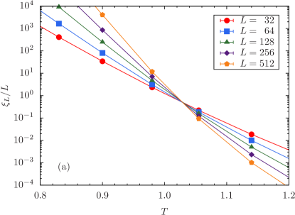
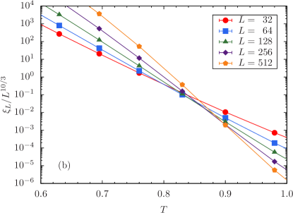
Figure 1: (Color online) (a) Critical scaling form $\xi_{L}/L$ vs temperature $T$ for the fully connected (complete) system with $\sigma=0.55$ in zero random field $H$. (b) Mean-field scaling form $\xi_{L}/L$ vs temperature $T$ for the fully connected (complete) system with $\sigma=0.55$ in zero random field $H$.

Figure 1 shows the two scaling forms based on critical scaling [Eq. (6)] and the mean-field scaling form expected above the upper critical dimension [Eq. (8)]. We had expected that the crossing of the curves for different $L$ values would have been superior for the mean-field scaling form, but this is clearly not the case for the studied system sizes. A similar behavior when searching for the AT line was found by Angelini and Biroli in Ref. Angelini and Biroli, 2015 and they suggested as a consequence that $d_{u}$ might not be $6$ for spin glasses in a field and that the critical behavior for $d>6$ might not be controlled by the Gaussian fixed point but by some (as yet) undetermined nonperturbative fixed point.

If one believes in the conventional wisdom that $6$ is the upper critical dimension both in zero field and for the AT, then the only possible explanation for the poor mean-field scaling is large corrections to scaling in Fig. 1. On this explanation, if one could obtain data for much larger systems than $L=512$, then the crossing with mean-field scaling would eventually become better than that for critical scaling. We cannot obtain such data for the fully connected system, but we can for the diluted model and the results for the two kinds of scaling functions are shown in Fig. 2.

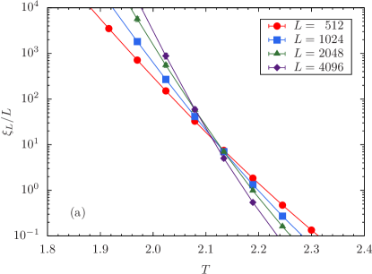
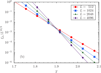
Figure 2: (Color online) (a) Critical scaling form $\xi_{L}/L$ vs temperature $T$ for the diluted model with $\sigma=0.55$ in zero random field $H$. (b) Mean-field scaling form $\xi_{L}/L$ vs temperature $T$ for the diluted model with $\sigma=0.55$ in zero random field $H$.

There is some evidence that the crossing is indeed improving for the mean-field scaling in these larger systems, but one could not really argue that it is superior to the critical scaling form. Hence, using these simple scaling plots we are unable to provide strong evidence for $d_{u}=6$. Instead, we have to resort to an alternate approach to show that mean-field scaling is the correct description of the critical behavior. Our approach is to analytically determine the scaling function $\tilde{\xi}\left[(T-T_{c})L^{1/3}\right]$ and show that the simulational data fits well to this analytically calculated form. We find that it is possible to do this in zero field and we believe that this is good evidence for the validity of mean-field scaling. In a field, finite-size effects are even larger in numerical work and on the analytical side we have only been able to extract the asymptotic forms for the scaling functions.

Rather than study the scaling function $\tilde{\xi}$, it is simpler to study the equivalent scaling function for the spin-glass susceptibility $\chi_{\rm SG}(0)$ obtained from the second moment of the spin-glass order parameter $q$ where

$$q=\frac{1}{N}\sum_{i}S_{i}^{(1)}S_{i}^{(2)}.$$ (9)

Here “(1)” and “(2)” refer to two independent copies of the system with the same interactions $J_{ij}$. We have studied in particular the second moment $q_{2}=[\langle q^{2}\rangle]_{\rm av}$ and the quantity

$$\chi_{\rm SG}=N[\langle q^{2}\rangle]_{\rm av}$$ (10)

which is the spin-glass susceptibility in zero field. (Note that in a finite system in zero field $\langle S_{i}\rangle=0$.) The analog of the mean-field scaling form in Eq. (8) is Wittmann and Young (2012)

$$\chi_{\rm SG}/L^{1/3}=\tilde{\chi}\left[(T-T_{c})L^{1/3}\right].$$ (11)

The analog of the critical scaling of Eq. (6) is Wittmann and Young (2012)

$$\chi_{\rm SG}/L^{2-\eta}=\tilde{\chi}\left[(T-T_{c})L^{1/\nu}\right],$$ (12)

where $2-\eta=2\sigma-1$. Again, $\tilde{\chi}(x)$ denotes the scaling function, which will also be called $f(x)$. The advantage of studying $\chi_{\rm SG}$ rather than $\xi_{L}$ is that we can study it in the SK universality class where $\sigma<1/2$, whereas $\xi_{L}$ is ill-defined for these values of $\sigma$. The crossing of $\chi_{\rm SG}/L^{1/3}$ when plotted against the temperature $T$ for various values of the system size $L$ were studied in Ref. Wittmann and Young, 2012 for $\sigma=0$ and $0.25$. For $\sigma=0.55$ we present in Fig. 3 the corresponding scaling plots.

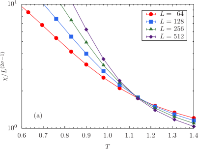
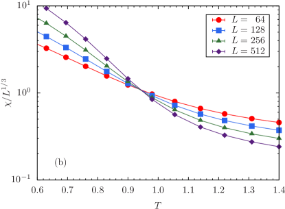
Figure 3: (Color online) (a) Critical scaling form of the susceptibility $\chi/L^{2\sigma-1}$ vs temperature $T$ for the fully connected (complete) system with $\sigma=0.55$ when the random field $H=0$. (b) Mean-field scaling form $\chi/L^{1/3}$ of the susceptibility $\chi/L^{2\sigma-1}$ vs temperature $T$ for the fully connected (complete) system with $\sigma=0.55$ when the random field $H=0$. Note that $\chi\equiv\chi_{\rm SG}$.

Notice that in the case of the susceptibility the quality of the crossing is comparable for both the mean-field and critical scaling, whereas for the correlation length the critical scaling form seemed superior, at least for the fully connected system. However, the temperature at which the curves cross provides an estimate of $T_{c}$, and for both $\chi_{\rm SG}$ and $\xi_{L}$ critical scaling is indicating a $T_{c}>1$, whereas mean-field scaling indicates a $T_{c}<1$. At the level of mean-field theory the transition temperature would be $T_{c}=1$, and the fluctuations about the mean field normally reduce the value of the critical temperature $T_{c}$. This clearly is an argument in favor of using the mean-field scaling form. The same observation can be made for the diluted model. For it the mean-field transition temperature is $2.0564$ Wittmann and Young (2012), and the estimate of $T_{c}$ in Fig. 2 for the case of $\sigma=0.55$ is certainly less than this number using mean-field scaling, but larger than this for the critical scaling form.

Standard finite-size scaling for mean-field scaling takes the form Wittmann and Young (2012)

$$\chi_{\rm SG}(T,L) = L^{1/3}\left[f(L^{1/3}t)+L^{-\omega}g(L^{1/3}t)+\cdots\right]$$ (13)

$$+ d_{0}L^{2\sigma-1}h(L^{1/3}t)+c_{0}+c_{1}t+\cdots,$$

where $t=T/T_{c}-1$, and the correction-to-scaling exponent is $\omega=2-3\sigma$ Kotliar et al. (1983). In the limit $L\to\infty$ with $L^{1/3}t$ fixed, this equation reduces to the simpler form

$$\chi_{\rm SG}/L^{1/3}=f(L^{1/3}t)$$ (14)

as then the corrections to scaling become negligible. In what follows, we shall refer to the limit with $x=L^{1/3}t$ fixed as “$L\to\infty$” as the finite-size scaling limit, and “$f(x)$” as the finite-size scaling function for $\chi_{\rm SG}/L^{1/3}$.

In Sec. III we outline the Brézin and Zinn-Justin procedure Brézin and Zinn-Justin (1985) for calculating the universal scaling function $f(x)$ for any space dimension $d>d_{u}=6$ (or $\sigma<2/3$) and show that our simulational data at $\sigma=0.0$, $0.25$, and $0.55$ are consistent with being in the same universality class. In Sec. IV we determine $f(x)$ by using the mean-field equations of Thouless, Anderson and Palmer (TAP) Thouless et al. (1977), as modified by Plefka (TAPP) Plefka (2002). We shall use in Sec. V these same equations to determine the analog of the scaling function $f(x)$ at the AT transition in nonzero field, however only in the limit of large $x$. Finally, in Sec. VI we discuss finite-size problems which might make one believe there is an AT line for $d\leq 6$ ($\sigma\geq 2/3$) even though it is absent.

III Universality of the finite-size scaling function for $\sigma<2/3$

If the critical behavior is controlled by the Gaussian fixed point, Brézin and Zinn-Justin Brézin and Zinn-Justin (1985) showed how the finite-size scaling function $f(x)$ can, in principle, be calculated. The procedure basically reduces to calculating the integral

$$\overline{Z^{n}}=\int dQ_{\alpha\beta}\exp\left[-F[\{Q_{\alpha\beta}\}]/kT\right],$$ (15)

where

$$F[\{Q_{\alpha\beta}\}]/kT = \int d^{d}x\,\left[\frac{1}{2}r\sum_{\alpha<\beta}Q_{\alpha\beta}^{2}\right.$$ (16)

$$+\left.\frac{w}{6}\sum_{\alpha<\beta<\gamma}Q_{\alpha\beta}Q_{\beta\gamma}Q_{\gamma\alpha}+{\mathcal{O}}(Q^{4})\right].$$

The coefficient $r$ is essentially a measure of the distance from $T_{c}$, i.e., it is related to the reduced temperature $t$. The $Q^{4}$ terms are irrelevant when calculating the scaling function, as are the usual density gradient terms $(\nabla Q_{\alpha\beta})^{2}$ seen in such free-energy functionals Harris et al. (1976), although they would have been needed if we had tried to calculate the scaling function associated with $\xi_{L}$. $Q_{\alpha\beta}$ is related to the spin-glass order parameter, and $\alpha$ takes the values $1$, $2$, $\cdots$, $n$, with $n\to 0$. This integral should be adequate for calculating the crossover scaling function $f(x)$ in the mean-field scaling regime, i.e., for all $\sigma<2/3$. The form of the function is universal, and the differences between fully connected spins or the diluted version of the model, or the value of $\sigma$, just feed into the value of $T_{c}$, the overall amplitude of $\chi_{\rm SG}/L^{1/3}$, and a multiplicative factor associated with $t$. For $\sigma>2/3$, when the behavior is not controlled by the Gaussian fixed point but instead by the critical fixed point Harris et al. (1976), the calculation of the scaling function is more complicated. Its argument changes to $L^{1/\nu}t$ and the scaling function is different from the universal form expected to apply for all $\sigma<2/3$.

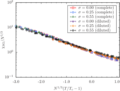
Figure 4: (Color online) Reduced spin-glass susceptibility $\chi_{\rm SG}/N^{1/3}$ vs $x=N^{1/3}(T/T_{c}-1)$, (recall, $N\equiv L$), i.e., the finite-size scaling function $f(x)$ in zero field for all system sizes $N$ studied. For the SK model ($\sigma=0$) we simulated $N=1024,\ldots,4096$. For the diluted model and $\sigma=0$ we studied $N=2048,\ldots,16384$. For $\sigma=0.25$ we studied $N=512,\ldots,4096$ for the complete (fully connected) model and $N=2048,\ldots,16384$ for the diluted model. Data taken from Ref. Wittmann and Young, 2012. For $\sigma=0.55$ we studied $N=32,\ldots,512$ for the complete (fully connected) model and $N=128,\ldots,2048$ for the diluted model. Data taken from Refs. Katzgraber and Young, 2003a and Katzgraber et al., 2009. For $\sigma=0.55$ for the complete (fully connected) case we have taken $T_{c}\approx 0.94$, while for the diluted case we use $T_{c}\approx 1.98$. Note the vertical logarithmic scale.

In Fig. 4 we plot results for $\chi_{\rm SG}/N^{1/3}$ vs the scaling variable $x=(T/T_{c}-1)N^{1/3}$ for $\sigma=0.0$, $0.25$, and $0.55$ for both the fully connected (complete) model and for the diluted model. The points include data for all the system sizes $N$ simulated (see caption). In the range $1>x>-3$ there is a fairly satisfactory collapse of the data onto a single curve for the differing values of $\sigma$ and for both the fully connected and dilute models. None of the data have been linearly scaled on either the horizontal or vertical axes of the figure, which would have been permissible while staying in the same universality class. The data for $x>1$ are strongly affected by finite-size effects, some of which can be seen in Fig. 5, which is why in Fig. 4 we have limited the horizontal range to $x<1$.

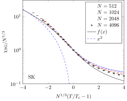
Figure 5: (Color online) Reduced spin-glass susceptibility $\chi_{\rm SG}/N^{1/3}$ vs $x=N^{1/3}(T/T_{c}-1)$, i.e., the finite-size scaling function $f(x)$ in zero field for the SK model ($\sigma=0$). The data are taken from Ref. Wittmann and Young, 2012. For this model $T_{c}=1$ Sherrington and Kirkpatrick (1975). The data for $x>1$ are strongly affected by finite-size effects. The solid curve shows our approximation based on Eq. (29) for the scaling function $f(x)$ based on solving the TAPP equations. It gives, at large positive $x$, $f(x)\to 1/(2x)$, while at large negative $x$, $f(x)\to x^{2}$. The blue dashed curve is the asymptotic limit $f(x)\to x^{2}$ for negative $x$ values.

Overall the data are consistent with a universal scaling function $f(x)$ for $\sigma<2/3$. If the behavior were controlled by a nonperturbative fixed point rather than by the Gaussian fixed point, then such universality of $f(x)$ would have to be understood. Furthermore, as we shall see in Sec. IV below, it is possible to calculate the function $f(x)$ explicitly. Our results in Fig. 5 turn out to be in satisfactory agreement with our approximation.

It is possible to determine the behavior of $f(x)$ as $x\to\pm\infty$ by simple arguments: when $x\to-\infty$, $\chi_{\rm SG}\to Nq^{2}$, and as $q\to-t$ in the scaling limit where $t\to 0$, that means that $f(x)\to x^{2}$. The data in Fig. 5 are approaching this estimate at large negative $x$. For $x\to\infty$, $\chi_{\rm SG}\to 1/(1-\beta^{2})$ [see Eq. (25)] for the SK model and also from the TAPP equations, which implies that $f(x)\to 1/(2x)$ as $\beta=1/(1+t)$. Again, the data shown in Fig. 5 seem to be approaching this limit, but the finite-size effects are large for positive $x$. This is not due to any inaccuracies in the TAPP equations, but just points to the fact that in order to use the simplification $\chi_{\rm SG}=1/(2t)$ [which leads to $f(x)\to 1/(2x)$] one needs to work with rather small values of $t$. However, at fixed large $x$, this requires working with very large values of $N$, which are currently not accessible numerically.

IV Calculation of the scaling function $f(x)$

In this section we outline how one can calculate the finite-size scaling function $f(x)$. One approach would be to simply do the integrals in Eq. (15). Unfortunately, that is very difficult because of the replica labels and the need to continue $n\to 0$. However, an approach equivalent to this was used by three of us in Ref. Yeo et al., 2005 and it results in studying the finite-size scaling function for the spherical SK spin-glass model, which according to the arguments in the aforementioned reference should have an identical scaling function $f(x)$. However, this approach is hard to extend to the behavior in a field, so instead we present an approach which does permit, in principle, an extension to finite fields.

Assuming that the scaling function $f(x)$ applies for all $\sigma<2/3$, if we can calculate it for the SK model with $\sigma=0$ and that agrees with data for (say) $\sigma=0.55$—as is the case in Fig. 4—then the assumption would seem to be correct. To calculate $f(x)$ for the SK model we use the TAP equations Thouless et al. (1977) as modified by Plefka Plefka (2002) and refer to them as the TAPP equations. Plefka argued that in the presence of an external field $h_{i}$ at each site $i$, the magnetization $m_{i}$ is given by

$$m_{i}=\tanh\beta\big{[}h_{i}+\sum_{j}J_{ij}m_{j}-m_{i}\chi_{\ell}\big{]},$$ (17)

where the local susceptibility is given by

$$\chi_{\ell}=N^{-1}\sum_{i}\chi_{ii}=N^{-1}\sum_{i}\partial m_{i}/\partial h_{i}.$$ (18)

Plefka assumed that $\partial\chi_{\ell}/\partial m_{i}$ is of order ${\mathcal{O}}(N^{-1})$ and thus negligible when the inverse susceptibility matrix is calculated from Eq. (17)

$$\chi_{ij}^{-1}=\delta_{ij}[\beta^{-1}(1-m_{i}^{2})^{-1}+\chi_{\ell}]-J_{ij}.$$ (19)

Equations (17) and (19), with $\sum_{j}\chi_{ij}\chi_{jk}^{-1}=\delta_{ik}$ form a closed set of equations for the $m_{i}$ and $\chi_{\ell}$. They are not exact, unfortunately, as the terms of ${\mathcal{O}}(N^{-1})$ can, for certain quantities, combine to make ${\mathcal{O}}(1)$ contributions Aspelmeier et al. (2004). We believe that such possibilities are unimportant in our calculation of $f(x)$. Our argument for this is that the use of these equations gives in our finite-size scaling limit the same results as can be obtained by the spherical model SK spin glass mapping Yeo et al. (2005), which we think is exact in zero field. For zero fields, in our scaling regime, $m_{i}\to 0$, and Eq. (19) simplifies to

$$\chi_{ij}^{-1}=\delta_{ij}[\beta^{-1}+\chi_{\ell}]-J_{ij}.$$ (20)

The self-consistency equation for $\chi_{\ell}$ is then conveniently written in terms of $z=\beta^{-1}+\chi_{\ell}$ as

$$z-\beta^{-1}=N^{-1}\sum_{i}\frac{1}{z-\lambda_{i}},$$ (21)

where $\lambda_{i}$ are the eigenvalues of the matrix $J_{ij}$. The physical solution is the solution which has the largest real value of $z$.

In the large-$N$ limit, the $N$ real eigenvalues $\lambda_{i}$ are described by the semicircle distribution with support between $-2$ and $2$. Then Eq. (21) reduces to

$$z-\beta^{-1}=1+\frac{(z-2)-\sqrt{(z-2)(z+2)}}{2},$$ (22)

which gives $z=\beta+\beta^{-1}$. We want to calculate

$$\chi_{\rm SG} \equiv \frac{1}{\beta^{2}}N^{-1}\sum_{i,j}\chi_{ij}^{2}$$ (23)

$$= \frac{1}{\beta^{2}}N^{-1}\sum_{i}\frac{1}{(z-\lambda_{i})^{2}}.$$

In the large-$N$ limit, the sum can be done and gives

$$\frac{1}{2\beta^{2}}\cdot\frac{z}{\sqrt{z^{2}-4}-1},$$ (24)

which reduces to

$$\chi_{\rm SG}\to\frac{1}{1-\beta^{2}},$$ (25)

on substituting $z=\beta+\beta^{-1}$. It is this result which we use to determine the limit of $f(x)$ as $x\to\infty$ (see Fig. 6).

In principle, for finite $N$ values, one could solve for $z$ numerically using Eq. (21). However, this is difficult for large $N$. Instead, we give an approximate solution which seems in practice to be quite accurate. As $x\to-\infty$, $z\to\lambda_{\rm max}$ and throughout the scaling region differs from $\lambda_{\rm max}$ by terms of ${\mathcal{O}}(1/N^{2/3})$. The largest eigenvalue itself has the form $\lambda_{\rm max}=2+{\mathcal{O}}(1/N^{2/3})$. Let us introduce the variable $u=(z-\lambda_{\rm max})N^{2/3}>0$ and the notation $\Delta=(\lambda_{\rm max}-\lambda_{1})N^{2/3}$, where $\lambda_{1}$ is the next largest eigenvalue. Then we separate off the first two terms in the sum in Eq. (21) and approximate the rest by Eq. (22) after replacing $(z-2)$ by $(z-\lambda_{\rm max})$ Yeo et al. (2005). The left-hand side of Eq. (21) becomes

$$z-\beta^{-1}\to 1-x/N^{1/3}+{\mathcal{O}}(1/N^{2/3}).$$ (26)

The right-hand side becomes

$$\frac{1}{N^{1/3}u}+\frac{1}{N^{1/3}(u+\Delta)}+1-\sqrt{u/N^{2/3}}+{\mathcal{O}}(1/N^{2/3}).$$ (27)

Thus, correct to ${\mathcal{O}}(1/N^{2/3}),$ we have as our basic approximation for $u$,

$$-x=\frac{1}{u}+\frac{1}{u+\Delta}-\sqrt{u}.$$ (28)

Within the same approximation, the sample with gap $\Delta$ gives for $f(x)$

$$f(x)=\frac{1}{u^{2}}+\frac{1}{(u+\Delta)^{2}}+\frac{1}{2\sqrt{u}}.$$ (29)

To calculate the bond-averaged value of $f(x)$ we must average over the spacing $\Delta$ which we do with the Wigner surmise distribution for it Rodgers and Moore (1989).

Before comparing with the numerical data we need to introduce the pseudocritical temperature $T_{c}(N)$ Billoire et al. (2011); Castellana et al. (2011). If one studies the function $-f^{\prime}(x)/f(x)$, it has a peak at $T_{c}$. However, in a system of finite size $N$, this peak is shifted to $T_{c}(N)$, where in the mean-field regime,

$$T_{c}(N)=T_{c}-\frac{a}{N^{1/3}}.$$ (30)

For the SK model $T_{c}=1$ and typical values for $a$ are $\sim 0.2$, but this depends on the function being studied Billoire et al. (2011). When trying to construct the universal scaling function $f(x)$ for different models it is natural to shift the horizontal axis so that the peaks for the different models coincide at $x=0$, which can by done by redefining $x$ so that $x=[T/T_{c}(N)-1]N^{1/3}$. This definition of $x$ differs from the old definition by $a+{\mathcal{O}}(1/N^{1/3})$. Thus, when comparing to our numerical data, one can shift the curves by an amount $a$ to improve the fit, and this is what we did in Fig. 5. With this shift, the overall agreement is quite satisfactory, considering the simplicity of the approximation. We suspect that it might be possible to calculate $f(x)$ exactly, but that remains a challenge for the future.

V Finite-size scaling at the Almeida-Thouless transition

In this section we shall discuss finite-size scaling at the AT transition de Almeida and Thouless (1978). The upper critical dimension of the AT line is expected to be the same as in zero field, that is, $d_{u}=6$ Bray and Roberts (1980). For the long-range model, that translates to $\sigma=2/3$. Note that in a field $\langle S_{i}\rangle$ is nonzero, and we have to study the cumulant second moment, i.e.,

$$\chi_{\rm SG}=\frac{1}{N}\sum_{i,j}\big{[}\langle S_{i}S_{j}\rangle-\langle S_{i}\rangle\langle S_{j}\rangle\big{]}_{\rm av}^{2}.$$ (31)

In a field we only have numerical data for the one-dimensional long-range model with $\sigma=0.55$. In Fig. 6 we show the mean-field scaling form $\chi_{\rm SG}/N^{1/3}=f_{H}(x)$ against $x=N^{1/3}[T/T_{c}(H)-1]$. The finite-size effects are strongly visible on the low-temperature side of the transition.

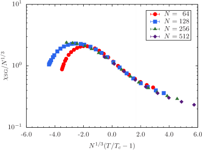
Figure 6: (Color online) Reduced spin-glass susceptibility $\chi_{\rm SG}/N^{1/3}$ vs $x=N^{1/3}[T/T_{c}(H)-1]$, that is the finite-size scaling function $f_{H}(x)$ in a random field of standard deviation $0.10$ when $\sigma=0.55$. For this model $T_{c}(H=0.1)\approx 0.815$.

We now turn to understanding the form of the finite-size scaling function $f_{H}(x)$ near the AT transition. At the formal level, the analog of Eq. (16) for the AT transition involves just the fields in the replicon sector $\tilde{Q}_{\alpha\beta}$, which are such that $\sum_{\beta}\tilde{Q}_{\alpha\beta}=0$ Bray and Roberts (1980). The replicated partition function is

$$\overline{Z^{n}}=\int d\tilde{Q}_{\alpha\beta}\exp\left[-F[\{\tilde{Q}_{\alpha\beta}\}]/kT\right],$$ (32)

where the effective functional is

$$F[\{\tilde{Q}_{\alpha\beta}\}]/kT =\int d^{d}x\,\left[\frac{1}{4}\tilde{r}\sum\tilde{Q}_{\alpha\beta}^{2}\right.$$ (33)

$$+ \left.\frac{w_{1}}{6}\sum\tilde{Q}_{\alpha\beta}\tilde{Q}_{\beta\gamma}\tilde{Q}_{\gamma\alpha}+\frac{w_{2}}{6}\sum\tilde{Q}_{\alpha\beta}^{3}\right].$$

Here the convention has been adopted that the sums over replica indices are unrestricted. Note that $\tilde{Q}_{\alpha\alpha}=0$. At the AT line, $\tilde{r}=0$ in the mean-field approximation and the two couplings $w_{1}$ and $w_{2}$ both depend on the field $H$. We would expect as a consequence the finite-size scaling function $f_{H}(x)$ to depend on both $x$ and the strength of the field $H$. It is because the effective field theory is a cubic field theory that the upper critical dimension $d_{u}=6$ for the AT line Bray and Roberts (1980). Unfortunately, the integrals in Eq. (33) needed to calculate $f_{H}(x)$ are even more difficult to do than those of the zero-field case and other methods have to be used to understand the finite-size scaling function $f_{H}(x)$.

We have tried solving the TAPP equations for the SK limit in the presence of a field numerically. We obtained the solution for a given bond and field realization at high temperatures, and followed the solution down to lower temperatures, for $N$ values up to $400$. At temperatures well above $T_{c}(H)$, we obtained values for $\chi_{\rm SG}$ consistent with those in Fig. 6. At large positive values of $x$ one is effectively in the regime where one can use the locator expansion Bray and Moore (1979) on the TAPP equations. The result Plefka (2002) is that Eq. (25) is generalized to

$$\chi_{\rm SG}\to\frac{\chi_{\rm SG}^{0}}{1-\beta^{2}\chi_{\rm SG}^{0}},$$ (34)

where Sharma and Young (2010)

$$\chi_{\rm SG}^{0}=\frac{1}{N}\sum_{i}(1-m_{i}^{2})^{2}.$$ (35)

We stress that this result holds just for the large-$N$ limit and $T>T_{c}(H)$. For the SK model in a random field $H$, $\chi_{\rm SG}^{0}$ can be determined explicitly. At the AT transition $T_{c}(H)$, $\chi_{\rm SG}^{0}=T_{c}(H)^{2}$, and so for $T$ close to $T_{c}(H)$,

$$\chi_{\rm SG}\to\frac{T_{c}(H)^{2}}{[1-\beta T_{c}(H)][1+\beta T_{c}(H)]}\to\frac{1}{2t}T_{c}(H)^{2},$$ (36)

where $t=[T/T_{c}(H)-1]$. For $H=0.1$, $T_{c}(0.1)=0.819428$ for the SK model, so $\chi_{\rm SG}\to 0.33573/t$. Unfortunately, the data in Fig. 6 have not been obtained at large enough values of $N$ (here the largest $N$ value is $512$) or small enough values of $t$, to see this behavior clearly. However, the calculated values of $\chi_{\rm SG}$ are consistent with the result presented in Eq. (34).

As the temperature is reduced to well below $T_{c}(H)$, the solution of the TAPP equations in the large-$N$ limit is expected to reduce to $\chi_{\rm SG}\to 1/|t|$ Plefka (2002). For the $N$ values for which we could obtain solutions, i.e., $N<400$, this behavior was not visible. In fact, most samples showed a peak in $\chi_{\rm SG}$ well above $T_{c}(H)$, followed by a fall at lower temperatures. We suspect that the fall at low temperatures visible in Fig. 6 might by connected with the fall seen in the TAPP equations. The decrease in $\chi_{\rm SG}/N^{1/3}$ at large negative $x$ values seen in Fig. 6 is clearly a finite-size effect.

We suspect that in the absence of finite-size effects $f_{H}(x)$ would actually continue to grow $\propto x^{2}$ at large negative $x$, due to replica symmetry breaking effects de Dominicis et al. (2005), and not follow the expectations based on the solution of the TAPP equations, which would be that $f(x)\to 1/|x|$. In Ref. de Dominicis et al., 2005 it was shown that for the SK model, where the Parisi RSB broken order parameter is $q(x)$,

$$\chi_{\rm SG}=\frac{N}{3}\left\{\int_{0}^{1}q^{2}(x)dx-\left[\int_{0}^{1}q(x)dx\,\right]^{2}\right\}.$$ (37)

At large negative $x$ one would therefore expect that because of these replica symmetry breaking effects that $f_{H}(x)\to Bx^{2}$ so that $\chi_{\rm SG}$ is proportional to $N$. Using the results in Refs. de Dominicis et al., 2005 and Thouless et al., 1980 for $q(x)$ in a field, one can calculate the coefficient $B$ and it is of order $q_{EA}$ on the AT line, which is small ($\approx 0.2)$ when $H=0.1$. However, the data in Fig. 6 at negative $x$ values are not extensive enough to provide a clear verification of these predictions.

VI Numerical searches for the Almeida-Thouless line when $d\leq 6$ ($\sigma\geq 2/3$)

In Sec. I we stated that there is likely no AT line when $d\leq 6$. As a consequence, we were surprised when Castellana and Parisi Castellana and Parisi (2015) recently claimed that in the Dyson hierarchical model numerical evidence suggested the existence of an AT line at $\sigma=0.68>2/3$ which corresponds to an effective space dimension $d<6$. At the transition they reported values for the critical exponents which were not close to their mean-field values, which lead them to suggest that the behavior was being controlled by a nonperturbative fixed point.

In this section we discuss a problem which arises when trying to determine the existence of the AT line in dimensions where there might be no AT line. It is again a finite-size problem. If there is no AT line and the droplet picture applies, then the correlation length $\xi_{D}$ in the system is the Imry-Ma length Imry and Ma (1975), determined by equating the free energy cost of flipping a region of size $\xi_{D}$, $kT_{c}(\xi_{D}/\xi)^{\theta}$ to the energy which might be gained from the random applied field, which is $\sqrt{q}H\xi_{D}^{d/2}$ (see for example, Ref. Yeo and Moore, 2015). Here $\xi$ denotes the zero-field correlation length $\sim 1/|t|^{\nu}$. In our one-dimensional model, $\theta=1-\sigma$ Moore (2012). Then

$$\frac{\xi_{D}}{\xi}\sim\left[\frac{H_{\rm AT}}{H}\right]^{2/(2\sigma-1)},$$ (38)

where

$$H_{\rm AT}\equiv kT_{c}|t|^{(\gamma+\beta)/2},$$ (39)

which is the scaling expectation for the form of the AT line Yeo and Moore (2015), should it exist. At the borderline value of $\sigma=2/3$, $\xi_{D}$ grows rapidly for small fields $\propto 1/H^{6}$. In order to see droplet behavior one requires system sizes $L>\xi_{D}$. Otherwise, one might be tempted to think there is an AT line. For $\sigma=0.75$ we plot $\xi_{L}/L$ as a function of the field $H$ in Fig. 7. Here, $\xi_{D}$ grows at small $H$ $\propto 1/H^{4}$. Figure 7 shows that the droplet model prediction that $\xi_{L}\sim\xi_{D}$ fails when $\xi_{L}>L$, as then finite-size effects are clearly making $\xi_{L}$ deviate away from $\xi_{D}$. The basic message is that to see droplet model behavior one needs to study system sizes $L>\xi_{D}$. When studying fields where $\xi_{D}>L$, one can be misled into thinking there is evidence for an AT line, as discussed at great length in Ref. Larson et al., 2013. We suspect this is why the authors of Ref. Castellana and Parisi, 2015 thought there was an AT line at $\sigma=0.68$. In fact, the growth of $\xi_{D}$ as $1/H^{6}$ when $\sigma\to 2/3^{+}$ will always make it very difficult to obtain data for the regime where $L>\xi_{D}$.

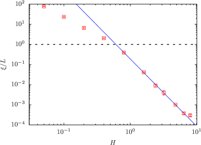
Figure 7: (Color online) Correlation length $\xi_{L}/L$ over a large range of field values for $L=1024$, $T=0.48$, and $\sigma=0.75$. The horizontal dashed line is a guide to the eye marking the point where $\xi_{L}=L$. A change in behavior for $\xi<L$ is apparent. The solid (blue) line marks the regime where the Imry-Ma argument Imry and Ma (1975) is valid.

VII Conclusions

We have studied finite-size effects on critical scaling in Ising spin glasses both in zero field and finite field in the regime where mean-field scaling is expected. We believe that the conventional wisdom that both types of transition have $6$ as the upper critical dimension is supported by the numerical data gathered from previous studies, even though strong finite-size effects are present. For the zero-field case, we have found a simple approximation for the crossover function for the spin-glass susceptibility. The finite-field case is far more difficult, but we have been able to determine the asymptotic form of the crossover function by allowing for the non-self-averaging features of the Parisi order parameter $q(x)$ which occur below the AT transition.

We should point out that there is a lack of self averaging generally throughout the critical scaling regime. Thus, in zero field, we have studied in the SK limit the distribution function of $\chi_{\rm SG}$ at $T=T_{c}$ which arises from different realizations of the bonds $J_{ij}$ that has a well-defined distribution. The zero-field problem seems sufficiently simple such that one day the scaling function $f(x)$ might be determined analytically; as a by-product one might then obtain the corresponding distribution functions.

We have argued previously that evidence for an AT line when $d<6$ might be just a consequence of not allowing for the effects of finite-size effects. In order to see the droplet picture emerging clearly, one needs the linear system size $L$ to be larger than the Imry-Ma length $\xi_{D}$. However, this length scale can be very long at the fields commonly used in most numerical studies. This means that when $L\leq\xi_{D}$ one can easily be mislead into believing that there is a transition in a field. For example, from the data presented in Fig. 7 for the one-dimensional model with $\sigma=0.75$, one needs system sizes $L$ larger than $1024$ sites, as well as fields stronger than $H_{R}\approx 0.7$ to see the droplet behavior. Our hope is that future studies first verify the needed system sizes $L>\xi_{D}$ before claiming the existence of a spin-glass state in a field.