Orthogonal polynomials for a class of measures with discrete rotational symmetries in the complex plane

F. Balogh Scuola Internazionale Superiore di Studi Avanzati, Trieste Concordia University, Montrรฉal T. Grava Scuola Internazionale Superiore di Studi Avanzati, Trieste School of Mathematics, University of Bristol D. Merzi Scuola Internazionale Superiore di Studi Avanzati, Trieste
( Correspondence to be sent to grava@sissa.it)
Abstract

We obtain the strong asymptotics of polynomials pnโ€‹(ฮป)subscript๐‘๐‘›๐œ†p_{n}(\lambda), ฮปโˆˆโ„‚๐œ†โ„‚\lambda\in\mathbb{C}, orthogonal with respect to measures in the complex plane of the form

eโˆ’Nโ€‹(|ฮป|2โ€‹sโˆ’tโ€‹ฮปsโˆ’tยฏโ€‹ฮปยฏs)โ€‹dโ€‹Aโ€‹(ฮป),superscript๐‘’๐‘superscript๐œ†2๐‘ ๐‘กsuperscript๐œ†๐‘ ยฏ๐‘กsuperscriptยฏ๐œ†๐‘ ๐‘‘๐ด๐œ†e^{-N(|\lambda|^{2s}-t\lambda^{s}-\overline{t}\overline{\lambda}^{s})}dA(\lambda),

where s๐‘ s is a positive integer, t๐‘กt is a complex parameter and dโ€‹A๐‘‘๐ดdA stands for the area measure in the plane. Such problem has its origin from normal matrix models. We study the asymptotic behaviour of pnโ€‹(ฮป)subscript๐‘๐‘›๐œ†p_{n}(\lambda) in the limit n,Nโ†’โˆžโ†’๐‘›๐‘n,N\to\infty in such a way that n/Nโ†’Tโ†’๐‘›๐‘๐‘‡n/N\to T constant. Such asymptotic behaviour has two distinguished regimes according to the topology of the limiting support of the eigenvalue distribution of the normal matrix model. If 0<|t|2<T/s0superscript๐‘ก2๐‘‡๐‘ 0<|t|^{2}<T/s, the eigenvalue distribution support is a simply connected compact set of the complex plane, while for |t|2>T/ssuperscript๐‘ก2๐‘‡๐‘ |t|^{2}>T/s the eigenvalue distribution support consists of s๐‘ s connected components. Correspondingly the support of the limiting zero distribution of the orthogonal polynomials consists of a closed contour contained in each connected component.

Our asymptotic analysis is obtained by reducing the planar orthogonality conditions of the polynomials to an equivalent system of contour integral orthogonality conditions. The strong asymptotics for the orthogonal polynomials is obtained from the corresponding Riemannโ€“Hilbert problem by the Deiftโ€“Zhou nonlinear steepest descent method.

1 Introduction

We study the asymptotics of orthogonal polynomials with respect to a family of measures supported on the whole complex plane. To set up the notation for the general case, let pnโ€‹(ฮป)subscript๐‘๐‘›๐œ†p_{n}(\lambda) denote the monic orthogonal polynomials of degree n๐‘›n such that

โˆซโ„‚pnโ€‹(ฮป)โ€‹pmโ€‹(ฮป)ยฏโ€‹eโˆ’Nโ€‹Wโ€‹(ฮป)โ€‹๐‘‘Aโ€‹(ฮป)=hn,Nโ€‹ฮดnโ€‹m,n,m=0,1,2,โ€ฆformulae-sequencesubscriptโ„‚subscript๐‘๐‘›๐œ†ยฏsubscript๐‘๐‘š๐œ†superscript๐‘’๐‘๐‘Š๐œ†differential-d๐ด๐œ†subscriptโ„Ž๐‘›๐‘subscript๐›ฟ๐‘›๐‘š๐‘›๐‘š012โ€ฆ\int_{\mathbb{C}}p_{n}(\lambda)\overline{p_{m}(\lambda)}e^{-NW(\lambda)}dA(\lambda)=h_{n,N}\delta_{nm},\quad n,m=0,1,2,\dots (1.1)

where W:โ„‚โ†’โ„:๐‘Šโ†’โ„‚โ„W:\mathbb{C}\to\mathbb{R} is called the external potential, N๐‘N is a positive parameter111For simplicity we use the simpler notation pnโ€‹(ฮป)subscript๐‘๐‘›๐œ†p_{n}(\lambda) instead of pn,Nโ€‹(ฮป)subscript๐‘๐‘›๐‘๐œ†p_{n,N}(\lambda), even though the orthogonal polynomials depend on the value of the scaling parameter N๐‘N., dโ€‹Aโ€‹(ฮป)๐‘‘๐ด๐œ†dA(\lambda) is the area measure in the complex plane and hn,Nsubscriptโ„Ž๐‘›๐‘h_{n,N} is the norming constant. The external potential is assumed to have sufficient growth at infinity so that the integrals in (1.1) are bounded.

Planar orthogonal polynomials satisfying (1.1) appear naturally in the context of normal matrix models [12] where one studies probability distributions of the form

Mโ†ฆ1๐’ตn,Nโ€‹eโˆ’Nโ€‹Trโก(Wโ€‹(M))โ€‹dโ€‹M,๐’ตn,N=โˆซ๐’ฉneโˆ’Nโ€‹Trโก(Wโ€‹(M))โ€‹๐‘‘M,formulae-sequencemaps-to๐‘€1subscript๐’ต๐‘›๐‘superscript๐‘’๐‘Tr๐‘Š๐‘€๐‘‘๐‘€subscript๐’ต๐‘›๐‘subscriptsubscript๐’ฉ๐‘›superscript๐‘’๐‘Tr๐‘Š๐‘€differential-d๐‘€M\mapsto\frac{1}{{\mathcal{Z}}_{n,N}}e^{-N\operatorname{Tr}(W(M))}dM,\qquad{\mathcal{Z}}_{n,N}=\int_{{\mathcal{N}}_{n}}e^{-N\operatorname{Tr}(W(M))}dM, (1.2)

where ๐’ฉNsubscript๐’ฉ๐‘{\mathcal{N}}_{N} is the algebraic variety of nร—n๐‘›๐‘›n\times n normal matrices

๐’ฉn={M:[M,Mโ‹†]=0}โŠ‚Matnร—nโก(โ„‚),subscript๐’ฉ๐‘›conditional-set๐‘€๐‘€superscript๐‘€โ‹†0subscriptMat๐‘›๐‘›โ„‚{\mathcal{N}}_{n}=\left\{M\ \colon\ [M,M^{\star}]=0\right\}\subset\operatorname{Mat}_{n\times n}(\mathbb{C}), (1.3)

and dโ€‹M๐‘‘๐‘€dM is the volume form induced on ๐’ฉnsubscript๐’ฉ๐‘›{\mathcal{N}}_{n} which is invariant under conjugation by unitary matrices. Since normal matrices are diagonalizable by unitary transformations, the probability density (1.2) can be reduced to the form [43]

1Zn,Nโ€‹โˆi<j|ฮปiโˆ’ฮปj|2โ€‹eโˆ’Nโ€‹โˆ‘j=1nTrโกWโ€‹(ฮปi)โ€‹dโ€‹Aโ€‹(ฮป1)โ€‹โ‹ฏโ€‹dโ€‹Aโ€‹(ฮปn),1subscript๐‘๐‘›๐‘subscriptproduct๐‘–๐‘—superscriptsubscript๐œ†๐‘–subscript๐œ†๐‘—2superscript๐‘’๐‘superscriptsubscript๐‘—1๐‘›Tr๐‘Šsubscript๐œ†๐‘–๐‘‘๐ดsubscript๐œ†1โ‹ฏ๐‘‘๐ดsubscript๐œ†๐‘›\dfrac{1}{Z_{n,N}}\prod_{i<j}|\lambda_{i}-\lambda_{j}|^{2}e^{-N\sum_{j=1}^{n}\operatorname{Tr}{W(\lambda_{i})}}dA(\lambda_{1})\cdots dA(\lambda_{n}),

where ฮปjsubscript๐œ†๐‘—\lambda_{j} are the complex eigenvalues of the normal matrix M๐‘€M and the normalizing factor Zn,Nsubscript๐‘๐‘›๐‘Z_{n,N}, called partition function, is given by

Zn,N=โˆซโ„‚nโˆi<j|ฮปiโˆ’ฮปj|2โ€‹eโˆ’Nโ€‹โˆ‘j=1nWโ€‹(ฮปi)โ€‹dโ€‹Aโ€‹(ฮป1)โ€‹โ‹ฏโ€‹dโ€‹Aโ€‹(ฮปn).subscript๐‘๐‘›๐‘subscriptsuperscriptโ„‚๐‘›subscriptproduct๐‘–๐‘—superscriptsubscript๐œ†๐‘–subscript๐œ†๐‘—2superscript๐‘’๐‘superscriptsubscript๐‘—1๐‘›๐‘Šsubscript๐œ†๐‘–๐‘‘๐ดsubscript๐œ†1โ‹ฏ๐‘‘๐ดsubscript๐œ†๐‘›Z_{n,N}=\int_{\mathbb{C}^{n}}\prod_{i<j}|\lambda_{i}-\lambda_{j}|^{2}e^{-N\sum_{j=1}^{n}W(\lambda_{i})}dA(\lambda_{1})\cdots dA(\lambda_{n}).

The statistical quantities related to eigenvalues can be expressed in terms of the orthogonal polynomials pnโ€‹(ฮป)subscript๐‘๐‘›๐œ†p_{n}(\lambda) defined in (1.1). In particular, the average density of eigenvalues is

ฯn,Nโ€‹(ฮป)=1nโ€‹eโˆ’Nโ€‹Wโ€‹(ฮป)โ€‹โˆ‘j=0nโˆ’11hjโ€‹|pjโ€‹(ฮป)|2.subscript๐œŒ๐‘›๐‘๐œ†1๐‘›superscript๐‘’๐‘๐‘Š๐œ†superscriptsubscript๐‘—0๐‘›11subscriptโ„Ž๐‘—superscriptsubscript๐‘๐‘—๐œ†2\rho_{n,N}(\lambda)=\frac{1}{n}e^{-NW(\lambda)}\sum_{j=0}^{n-1}\frac{1}{h_{j}}\left|p_{j}(\lambda)\right|^{2}. (1.4)

The partition function Zn,Nsubscript๐‘๐‘›๐‘Z_{n,N} can be written as a product of the normalizing constants

Zn,N=โˆj=0nhj,N.subscript๐‘๐‘›๐‘superscriptsubscriptproduct๐‘—0๐‘›subscriptโ„Ž๐‘—๐‘Z_{n,N}=\prod_{j=0}^{n}h_{j,N}. (1.5)

While the asymptotic density of eigenvalues can be studied using an approach from potential theory [49], the zero distribution of orthogonal polynomials remains an open issue for general potential weights despite general results in [51]. The density of eigenvalues ฯn,Nโ€‹(ฮป)subscript๐œŒ๐‘›๐‘๐œ†\rho_{n,N}(\lambda) converges (in the sense of measures) in the limit

nโ†’โˆž,Nโ†’โˆž,Nnโ†’1T,formulae-sequenceโ†’๐‘›formulae-sequenceโ†’๐‘โ†’๐‘๐‘›1๐‘‡n\to\infty\ ,\quad N\to\infty\ ,\quad\frac{N}{n}\to\frac{1}{T}\ , (1.6)

to the unique probability measure ฮผโˆ—superscript๐œ‡\mu^{*} in the plane which minimizes the functional [25, 35]

Iโ€‹(ฮผ)=โˆซโˆซlogโก|ฮปโˆ’ฮท|โˆ’1โ€‹dโ€‹ฮผโ€‹(ฮป)โ€‹๐‘‘ฮผโ€‹(ฮท)+1Tโ€‹โˆซWโ€‹(ฮป)โ€‹๐‘‘ฮผโ€‹(ฮป).๐ผ๐œ‡superscript๐œ†๐œ‚1๐‘‘๐œ‡๐œ†differential-d๐œ‡๐œ‚1๐‘‡๐‘Š๐œ†differential-d๐œ‡๐œ†I(\mu)=\int\!\!\!\!\int\log|\lambda-\eta|^{-1}d\mu(\lambda)d\mu(\eta)+\frac{1}{T}\int W(\lambda)d\mu(\lambda). (1.7)

The functional Iโ€‹(ฮผ)๐ผ๐œ‡I(\mu) in (1.7) is the Coulomb energy functional in two dimensions and the existence of a unique minimizer is a well-established fact under mild assumptions on the potential Wโ€‹(ฮป)๐‘Š๐œ†W(\lambda) [49]. If W๐‘ŠW is twice continuously differentiable and its Laplacian ฮ”โ€‹Wฮ”๐‘Š\Delta W is non-negative, the equilibrium measure is given by

dโ€‹ฮผโˆ—โ€‹(ฮป)=ฮ”โ€‹Wโ€‹(ฮป)โ€‹ฯ‡Dโ€‹(ฮป)โ€‹dโ€‹Aโ€‹(ฮป),๐‘‘superscript๐œ‡๐œ†ฮ”๐‘Š๐œ†subscript๐œ’๐ท๐œ†๐‘‘๐ด๐œ†d\mu^{*}(\lambda)=\Delta W(\lambda)\chi_{D}(\lambda)dA(\lambda),

where ฯ‡Dsubscript๐œ’๐ท\chi_{D} is the characteristic function of the compact support set D=suppโก(ฮผโˆ—)๐ทsuppsuperscript๐œ‡D=\operatorname{supp}(\mu^{*}). Sub-leading order corrections to the behaviour of the eigenvalues distribution ฯn,Nโ€‹(ฮป)subscript๐œŒ๐‘›๐‘๐œ†\rho_{n,N}(\lambda) as n,Nโ†’โˆžโ†’๐‘›๐‘n,N\to\infty and fluctuations in the bulk and at the boundary of the support D๐ทD have been considered in [9, 3, 42, 4, 5].

The measure ฮผโˆ—superscript๐œ‡\mu^{*} can be also uniquely characterized by the Eulerโ€“Lagrange conditions

Wโ€‹(ฮป)Tโˆ’2โ€‹โˆซlogโก|ฮปโˆ’ฮท|โ€‹dโ€‹ฮผโˆ—โ€‹(ฮท)+โ„“Dโ‰ฅ0๐‘Š๐œ†๐‘‡2๐œ†๐œ‚๐‘‘superscript๐œ‡๐œ‚subscriptโ„“๐ท0\dfrac{W(\lambda)}{T}-2\int\log|\lambda-\eta|d\mu^{*}(\eta)+\ell_{D}\geq 0 (1.8)

for all values ฮปโˆˆโ„‚๐œ†โ„‚\lambda\in\mathbb{C} with equality in (1.8) on the support222To be precise, the equality on the support is valid only up to a set of capacity zero [49]. of ฮผโˆ—superscript๐œ‡\mu^{*}. The Lagrange multiplier โ„“Dsubscriptโ„“๐ท\ell_{D} is called the (generalized) Robin constant. It is a non-trivial problem to determine the shape of the support set D๐ทD. In some cases this problem is called Laplacian growth. When the potential Wโ€‹(ฮป)๐‘Š๐œ†W(\lambda) is real analytic the boundary โˆ‚D๐ท\partial D is a finite union of analytic arcs with at most a finite number of singularities [48], see also [35].

There is only a handful of potentials Wโ€‹(ฮป)๐‘Š๐œ†W(\lambda) for which the polynomials pnโ€‹(ฮป)subscript๐‘๐‘›๐œ†p_{n}(\lambda) can be explicitly computed. The simplest example is Wโ€‹(ฮป)=|ฮป|2๐‘Š๐œ†superscript๐œ†2W(\lambda)=|\lambda|^{2} for which the orthogonal polynomials pnโ€‹(ฮป)subscript๐‘๐‘›๐œ†p_{n}(\lambda) are monomials of degree n๐‘›n, the constants hn,Nsubscriptโ„Ž๐‘›๐‘h_{n,N} and the average density of eigenvalues ฯn,Nsubscript๐œŒ๐‘›๐‘\rho_{n,N} can be computed explicitly in terms of the Gamma function. The matrix model associated to this potential is known as the Ginibre ensemble [31, 30] and the density of eigenvalues ฯn,Nsubscript๐œŒ๐‘›๐‘\rho_{n,N} converges to the normalized area measure on the disk of radius T๐‘‡\sqrt{T} centered at the origin. In general, for radially symmetric potentials W=Wโ€‹(|ฮป|)๐‘Š๐‘Š๐œ†W=W(|\lambda|), the orthogonal polynomials are always monomials and in the limit (1.6), the eigenvalue distribution is supported either on a disk or an annulus by the Single-ring Theorem of Feinberg and Zee [28], whose rigorous proof can be found in [32]. The correlation functions in this case have been studied in [12].

The harmonic deformation of the Gaussian case Wโ€‹(ฮป)=|ฮป|2+(harmonic)๐‘Š๐œ†superscript๐œ†2harmonicW(\lambda)=|\lambda|^{2}+(\mbox{harmonic}) has been intensively studied. In particular the potential Wโ€‹(ฮป)=|ฮป|2โˆ’tโ€‹(ฮป2+ฮป2ยฏ)๐‘Š๐œ†superscript๐œ†2๐‘กsuperscript๐œ†2ยฏsuperscript๐œ†2W(\lambda)=|\lambda|^{2}-t(\lambda^{2}+\bar{\lambda^{2}}) is associated to the Hermite polynomials for |t|<1/2๐‘ก12|t|<1/2. In the limit (1.6) the distribution of eigenvalues is the normalized area measure on an ellipse, while the distribution of the zeros of the orthogonal polynomials is given by the (rescaled) Wigner semicircle law with support between the two foci of the ellipse [23].

The normal matrix model with a general deformation Wโ€‹(ฮป)=|ฮป|2+Reโก(Pโ€‹(ฮป))๐‘Š๐œ†superscript๐œ†2Re๐‘ƒ๐œ†W(\lambda)=|\lambda|^{2}+\operatorname{Re}(P(\lambda)) where Pโ€‹(ฮป)๐‘ƒ๐œ†P(\lambda) is a polynomial of a fixed degree has first been considered in the seminal papers [47] and [54] (see also the review article [56]), where the connection with the Heleโ€“Shaw problem and integrable structure in conformal dynamic has been pointed out. More general potentials have been considered later in [55]. For such potentials, however, the matrix integrals have convergence issues in the complex plane and therefore a natural cut-off has been introduced in the work of Elbau and Felder [25]. In [24] the polynomials associated to such deformed Gaussian potentials have been studied and it was argued that the Cauchy transform of the limiting zero distribution of the orthogonal polynomials coincides with the Cauchy transform of the limiting eigenvalue distribution of the matrix model outside the support of the eigenvalues. Moreover, it was also conjectured in [24] that the zero distribution of the polynomials pnโ€‹(ฮป)subscript๐‘๐‘›๐œ†p_{n}(\lambda) is supported on tree-like segments (the mother body, see definition below) inside the compact set (the droplet) that attracts the eigenvalues of the normal matrix model.

For the external potential Wโ€‹(ฮป)=|ฮป|2+Reโก(tโ€‹ฮป3)๐‘Š๐œ†superscript๐œ†2Re๐‘กsuperscript๐œ†3W(\lambda)=|\lambda|^{2}+\operatorname{Re}(t\lambda^{3}), Bleher and Kuijlaars [11] defined polynomials orthogonal with respect to a system of unbounded contours on the complex plane, without any cut-off and which satisfy the same recurrence relation that is asymptotically valid for the orthogonal polynomials of Elbau and Felder. They then study the asymptotic distribution of the zeros of such polynomials confirming the predictions of [24]. Similar results were obtained for the more general external potential [38] Wโ€‹(ฮป)=|ฮป|2โˆ’Reโก(tโ€‹|ฮป|k)๐‘Š๐œ†superscript๐œ†2Re๐‘กsuperscript๐œ†๐‘˜W(\lambda)=|\lambda|^{2}-\operatorname{Re}(t|\lambda|^{k}), kโ‰ฅ2๐‘˜2k\geq 2 and |t|๐‘ก|t| sufficiently small so that the eigenvalue distribution of the matrix model has an analytic simply connected support. Cases in which the eigenvalue support has singularities were analyzed in [39] and [6]. In particular in the work [6] the external potential Wโ€‹(ฮป)=|ฮป|2โˆ’2โ€‹cโ€‹logโก|ฮปโˆ’a|๐‘Š๐œ†superscript๐œ†22๐‘๐œ†๐‘ŽW(\lambda)=|\lambda|^{2}-2c\log|\lambda-a| with c๐‘c and a๐‘Ža positive constants, has been studied and the strong asymptotics of the corresponding orthogonal polynomials has been derived both in the case in which the support of the eigenvalues distribution is simply connected (pre-critical case) or multiply connected (post-critical case) and critical transition was observed (see also [53, 7]). We remark that in the work [6], differently form the previous works, the zeros of the orthogonal polynomials do not always accumulate on a curve that corresponds to the mother-body of the domain where the eigenvalues of the normal matrix models are distributed.

In this work we study the strong asymptotic of the polynomials pnโ€‹(ฮป)subscript๐‘๐‘›๐œ†p_{n}(\lambda) orthogonal with respect to a density eโˆ’Nโ€‹Wโ€‹(ฮป)superscript๐‘’๐‘๐‘Š๐œ†e^{-NW(\lambda)} where the external potential is of the form Wโ€‹(ฮป)=|ฮป|2โ€‹sโˆ’tโ€‹ฮปsโˆ’tยฏโ€‹ฮปยฏs๐‘Š๐œ†superscript๐œ†2๐‘ ๐‘กsuperscript๐œ†๐‘ ยฏ๐‘กsuperscriptยฏ๐œ†๐‘ W(\lambda)=|\lambda|^{2s}-t\lambda^{s}-\bar{t}\bar{\lambda}^{s} with ฮปโˆˆโ„‚,๐œ†โ„‚\lambda\in\mathbb{C}, s๐‘ s a positive integer and tโˆˆโ„‚โˆ–{0}.๐‘กโ„‚0t\in\mathbb{C}\setminus\{0\}. By a simple rotation of the variable ฮป๐œ†\lambda the analysis can be reduced to the case of real and positive t๐‘กt. Therefore, without loss of generality, we may and do assume that tโˆˆโ„+๐‘กsubscriptโ„t\in\mathbb{R}_{+}, that is,

Wโ€‹(ฮป)=|ฮป|2โ€‹sโˆ’tโ€‹(ฮปs+ฮปยฏs)ฮปโˆˆโ„‚,sโˆˆโ„•,t>0,formulae-sequence๐‘Š๐œ†superscript๐œ†2๐‘ ๐‘กsuperscript๐œ†๐‘ superscriptยฏ๐œ†๐‘ formulae-sequence๐œ†โ„‚formulae-sequence๐‘ โ„•๐‘ก0W(\lambda)=|\lambda|^{2s}-t(\lambda^{s}+\bar{\lambda}^{s})\qquad\lambda\in\mathbb{C},\;s\in\mathbb{N},\quad t>0, (1.9)

and the associated orthogonality measure is

eโˆ’Nโ€‹(|ฮป|2โ€‹sโˆ’tโ€‹(ฮปs+ฮปยฏs))โ€‹dโ€‹Aโ€‹(ฮป)ฮปโˆˆโ„‚,sโˆˆโ„•,t>0.formulae-sequencesuperscript๐‘’๐‘superscript๐œ†2๐‘ ๐‘กsuperscript๐œ†๐‘ superscriptยฏ๐œ†๐‘ ๐‘‘๐ด๐œ†๐œ†โ„‚formulae-sequence๐‘ โ„•๐‘ก0e^{-N\left(|\lambda|^{2s}-t(\lambda^{s}+\bar{\lambda}^{s})\right)}dA(\lambda)\qquad\lambda\in\mathbb{C},\;s\in\mathbb{N},\quad t>0. (1.10)

Note that the potential Wโ€‹(ฮป)๐‘Š๐œ†W(\lambda) has a discrete rotational โ„คssubscriptโ„ค๐‘ \mathbb{Z}_{s}-symmetry. It was observed in [8] (see also [26]) that if a potential Wโ€‹(ฮป)๐‘Š๐œ†W(\lambda) can be written in the form

Wโ€‹(ฮป)=1sโ€‹Qโ€‹(ฮปs),๐‘Š๐œ†1๐‘ ๐‘„superscript๐œ†๐‘ W(\lambda)=\dfrac{1}{s}Q(\lambda^{s}),

the equilibrium measure for W๐‘ŠW can be obtained from the equilibrium measure of Q๐‘„Q by an unfolding procedure. In our particular case

Qโ€‹(u)=sโ€‹|u|2โˆ’sโ€‹tโ€‹(u+uยฏ)=sโ€‹|uโˆ’t|2โˆ’sโ€‹t2๐‘„๐‘ข๐‘ superscript๐‘ข2๐‘ ๐‘ก๐‘ขยฏ๐‘ข๐‘ superscript๐‘ข๐‘ก2๐‘ superscript๐‘ก2Q(u)=s|u|^{2}-st(u+\bar{u})=s|u-t|^{2}-st^{2}

corresponds to the Ginibre ensemble so that the equilibrium measure for the potential Q๐‘„Q is the normalized area measure of the disk

|uโˆ’t|=tc,tc=Ts,formulae-sequence๐‘ข๐‘กsubscript๐‘ก๐‘subscript๐‘ก๐‘๐‘‡๐‘ |u-t|=t_{c},\quad t_{c}=\sqrt{\dfrac{T}{s}},

where T๐‘‡T has been defined in (1.6). The equilibrium measure for W๐‘ŠW turns out the be equal to

dโ€‹ฮผโˆ—โ€‹(ฮป)=sฯ€โ€‹tc2โ€‹|ฮป|2โ€‹(sโˆ’1)โ€‹ฯ‡Dโ€‹(ฮป)โ€‹dโ€‹Aโ€‹(ฮป),๐‘‘superscript๐œ‡๐œ†๐‘ ๐œ‹superscriptsubscript๐‘ก๐‘2superscript๐œ†2๐‘ 1subscript๐œ’๐ท๐œ†๐‘‘๐ด๐œ†d\mu^{*}(\lambda)=\dfrac{s}{\pi t_{c}^{2}}|\lambda|^{2(s-1)}\chi_{D}(\lambda)dA(\lambda), (1.11)

where ฯ‡Dsubscript๐œ’๐ท\chi_{D} is the characteristic function of the support set

D:={ฮปโˆˆโ„‚,|ฮปsโˆ’t|โ‰คtc}.assign๐ทformulae-sequence๐œ†โ„‚superscript๐œ†๐‘ ๐‘กsubscript๐‘ก๐‘D:=\{\lambda\in\mathbb{C},\,\,|\lambda^{s}-t|\leq t_{c}\}. (1.12)

We observe that for t<tc๐‘กsubscript๐‘ก๐‘t<t_{c} the equation (1.12) describes a simply connected domain in the complex plane with uniformizing map from the exterior of the unit disk in the ฮพ๐œ‰\xi-plane to the exterior of D๐ทD given by

fโ€‹(ฮพ)=tc1sโ€‹ฮพโ€‹(1+ttcโ€‹1ฮพs)1s๐‘“๐œ‰superscriptsubscript๐‘ก๐‘1๐‘ ๐œ‰superscript1๐‘กsubscript๐‘ก๐‘1superscript๐œ‰๐‘ 1๐‘ f(\xi)=t_{c}^{\frac{1}{s}}\xi\left(1+\frac{t}{t_{c}}\frac{1}{\xi^{s}}\right)^{\frac{1}{s}}

with inverse

Fโ€‹(ฮป)=fโˆ’1โ€‹(ฮป)=tcโˆ’1sโ€‹ฮปโ€‹(1โˆ’tฮปs)1s.๐น๐œ†superscript๐‘“1๐œ†superscriptsubscript๐‘ก๐‘1๐‘ ๐œ†superscript1๐‘กsuperscript๐œ†๐‘ 1๐‘ F(\lambda)=f^{-1}(\lambda)=t_{c}^{-\frac{1}{s}}\lambda\left(1-\dfrac{t}{\lambda^{s}}\right)^{\frac{1}{s}}. (1.13)

For t>tc๐‘กsubscript๐‘ก๐‘t>t_{c} the domain defined by the equation (1.12) consists of s๐‘ s connected components which have a discrete rotational symmetry. For s=2๐‘ 2s=2 the domain D๐ทD is called Cassini oval. The boundary of D๐ทD, namely โˆ‚D๐ท\partial D can be identified with the real ovals of the Riemann surface ๐’ฎ๐’ฎ{\cal S} defined by ๐’ฎ:={(ฮป,ฮท)โˆˆโ„‚2,(ฮปsโˆ’t)โ€‹(ฮทsโˆ’t)=tc2}assign๐’ฎformulae-sequence๐œ†๐œ‚superscriptโ„‚2superscript๐œ†๐‘ ๐‘กsuperscript๐œ‚๐‘ ๐‘กsuperscriptsubscript๐‘ก๐‘2{\cal S}:=\{(\lambda,\eta)\in\mathbb{C}^{2},\;\;(\lambda^{s}-t)(\eta^{s}-t)=t_{c}^{2}\} which has genus (sโˆ’1)2superscript๐‘ 12(s-1)^{2}. Such Riemann surface does not coincide with the Schottky double of D๐ทD for s>2๐‘ 2s>2.

The boundary of the domain D๐ทD can be also expressed by the equation

ฮปยฏ=Sโ€‹(ฮป),Sโ€‹(ฮป)=(t+tc2ฮปsโˆ’t)1s.formulae-sequenceยฏ๐œ†๐‘†๐œ†๐‘†๐œ†superscript๐‘กsuperscriptsubscript๐‘ก๐‘2superscript๐œ†๐‘ ๐‘ก1๐‘ \bar{\lambda}=S(\lambda),\quad S(\lambda)=\left(t+\dfrac{t_{c}^{2}}{\lambda^{s}-t}\right)^{\frac{1}{s}}. (1.14)

The function Sโ€‹(ฮป)๐‘†๐œ†S(\lambda) is analytic in a neighbourhood of โˆ‚D๐ท\partial D and it is called the Schwarz function associated to โˆ‚D๐ท\partial D (see e.g. [18]).

Remark 1.1.

The domain D๐ทD is a quadrature domain [33] with respect to the measure dโ€‹ฮผโˆ—dsuperscript๐œ‡{\rm d}\mu^{*}. Indeed for any function hโ€‹(ฮป)โ„Ž๐œ†h(\lambda) analytic in a neighbourhood of D๐ทD one has, by applying Stokesโ€™ theorem and the Residue Theorem,

โˆซDhโ€‹(ฮป)โ€‹๐‘‘ฮผโˆ—โ€‹(ฮป)=12โ€‹ฯ€โ€‹iโ€‹tc2โ€‹โˆซโˆ‚Dhโ€‹(ฮป)โ€‹ฮปsโˆ’1โ€‹(Sโ€‹(ฮป))sโ€‹๐‘‘ฮป=โˆ‘k=0sโˆ’1ckโ€‹hโ€‹(ฮปk)subscript๐ทโ„Ž๐œ†differential-dsuperscript๐œ‡๐œ†12๐œ‹๐‘–superscriptsubscript๐‘ก๐‘2subscript๐ทโ„Ž๐œ†superscript๐œ†๐‘ 1superscript๐‘†๐œ†๐‘ differential-d๐œ†superscriptsubscript๐‘˜0๐‘ 1subscript๐‘๐‘˜โ„Žsubscript๐œ†๐‘˜\int_{D}h(\lambda)d\mu^{*}(\lambda)=\dfrac{1}{2\pi it_{c}^{2}}\int_{\partial D}h(\lambda)\lambda^{s-1}(S(\lambda))^{s}d\lambda=\sum_{k=0}^{s-1}c_{k}h(\lambda_{k})

where Sโ€‹(ฮป)๐‘†๐œ†S(\lambda) is the Schwarz function (1.14), ck=1ssubscript๐‘๐‘˜1๐‘ c_{k}=\dfrac{1}{s} and ฮปk=t1sโ€‹e2โ€‹ฯ€โ€‹iโ€‹kssubscript๐œ†๐‘˜superscript๐‘ก1๐‘ superscript๐‘’2๐œ‹๐‘–๐‘˜๐‘ \lambda_{k}=t^{\frac{1}{s}}e^{\frac{2\pi ik}{s}}.

1.1 Statement of results

The goal of this manuscript is to determine pointwise asymptotics of the polynomials pnโ€‹(ฮป)subscript๐‘๐‘›๐œ†p_{n}(\lambda) defined in (1.1) orthogonal with respect to the weight (1.10) in the two cases

  • โ€ข

    pre-critical: t<tc๐‘กsubscript๐‘ก๐‘t<t_{c};

  • โ€ข

    post-critical: t>tc๐‘กsubscript๐‘ก๐‘t>t_{c}.

The โ„คssubscriptโ„ค๐‘ \mathbb{Z}_{s}-symmetry of the orthogonality measure (1.10) is inherited by the corresponding orthogonal polynomials. Indeed the non-trivial orthogonality relations are

โˆซโ„‚pnโ€‹(ฮป)โ€‹ฮปยฏjโ€‹s+lโ€‹eโˆ’Nโ€‹Wโ€‹(ฮป)โ€‹๐‘‘Aโ€‹(ฮป)=0,j=0,โ€ฆ,kโˆ’1,formulae-sequencesubscriptโ„‚subscript๐‘๐‘›๐œ†superscriptยฏ๐œ†๐‘—๐‘ ๐‘™superscript๐‘’๐‘๐‘Š๐œ†differential-d๐ด๐œ†0๐‘—0โ€ฆ๐‘˜1\int_{\mathbb{C}}p_{n}(\lambda)\bar{\lambda}^{js+l}e^{-NW(\lambda)}dA(\lambda)=0,\quad j=0,\dots,k-1,

where k๐‘˜k and l๐‘™l are such that

n=kโ€‹s+l,0โ‰คlโ‰คsโˆ’1,formulae-sequence๐‘›๐‘˜๐‘ ๐‘™0๐‘™๐‘ 1n=ks+l,\qquad 0\leq l\leq s-1, (1.15)

i.e., the n๐‘›n-th monic orthogonal polynomial satisfies the relation

pnโ€‹(e2โ€‹ฯ€โ€‹isโ€‹ฮป)=e2โ€‹ฯ€โ€‹iโ€‹nsโ€‹pnโ€‹(ฮป).subscript๐‘๐‘›superscript๐‘’2๐œ‹๐‘–๐‘ ๐œ†superscript๐‘’2๐œ‹๐‘–๐‘›๐‘ subscript๐‘๐‘›๐œ†p_{n}(e^{\frac{2\pi i}{s}}\lambda)=e^{\frac{2\pi in}{s}}p_{n}(\lambda). (1.16)

It follows that there exists a monic polynomial qk(l)subscriptsuperscript๐‘ž๐‘™๐‘˜q^{(l)}_{k} of degree k๐‘˜k such that

pnโ€‹(ฮป)=ฮปlโ€‹qk(l)โ€‹(ฮปs).subscript๐‘๐‘›๐œ†superscript๐œ†๐‘™subscriptsuperscript๐‘ž๐‘™๐‘˜superscript๐œ†๐‘ p_{n}(\lambda)=\lambda^{l}q^{(l)}_{k}(\lambda^{s}).\quad (1.17)

Therefore the sequence of orthogonal polynomials {pnโ€‹(ฮป)}n=0โˆžsuperscriptsubscriptsubscript๐‘๐‘›๐œ†๐‘›0\{p_{n}(\lambda)\}_{n=0}^{\infty} can be split into s๐‘ s subsequences labelled by the remainder lโ‰กnmods๐‘™modulo๐‘›๐‘ l\equiv n\mod s, and the asymptotics along the different subsequences can be studied via the sequences of reduced polynomials

{qk(l)โ€‹(u)}k=0โˆž,l=0,1,โ€ฆ,sโˆ’1.formulae-sequencesuperscriptsubscriptsubscriptsuperscript๐‘ž๐‘™๐‘˜๐‘ข๐‘˜0๐‘™01โ€ฆ๐‘ 1\left\{q^{(l)}_{k}(u)\right\}_{k=0}^{\infty}\ ,\qquad l=0,1,\dots,s-1.

By a simple change of coordinates it is easy to see that the monic polynomials in the sequence {qk(l)}k=0โˆžsuperscriptsubscriptsubscriptsuperscript๐‘ž๐‘™๐‘˜๐‘˜0\{q^{(l)}_{k}\}_{k=0}^{\infty} are orthogonal with respect to the measure

|u|โˆ’2โ€‹ฮณโ€‹eโˆ’Nโ€‹(|u|2โˆ’tโ€‹uโˆ’tโ€‹uยฏ)โ€‹dโ€‹Aโ€‹(u),ฮณ:=sโˆ’lโˆ’1sโˆˆ[0,1),assignsuperscript๐‘ข2๐›พsuperscript๐‘’๐‘superscript๐‘ข2๐‘ก๐‘ข๐‘กยฏ๐‘ข๐‘‘๐ด๐‘ข๐›พ๐‘ ๐‘™1๐‘ 01|u|^{-2\gamma}e^{-N(|u|^{2}-tu-t\bar{u})}dA(u),\quad\gamma:=\frac{s-l-1}{s}\in[0,1), (1.18)

namely they satisfy the orthogonality relations

โˆซโ„‚qk(l)โ€‹(u)โ€‹uยฏjโ€‹|u|โˆ’2โ€‹ฮณโ€‹eโˆ’Nโ€‹(|u|2โˆ’tโ€‹uโˆ’tโ€‹uยฏ)โ€‹๐‘‘Aโ€‹(u)=0,j=0,โ€ฆ,kโˆ’1.formulae-sequencesubscriptโ„‚superscriptsubscript๐‘ž๐‘˜๐‘™๐‘ขsuperscriptยฏ๐‘ข๐‘—superscript๐‘ข2๐›พsuperscript๐‘’๐‘superscript๐‘ข2๐‘ก๐‘ข๐‘กยฏ๐‘ขdifferential-d๐ด๐‘ข0๐‘—0โ€ฆ๐‘˜1\int_{\mathbb{C}}q_{k}^{(l)}(u)\bar{u}^{j}|u|^{-2\gamma}e^{-N\left(|u|^{2}-tu-t\bar{u}\right)}dA(u)=0,\qquad j=0,\dots,k-1. (1.19)

As a result of this symmetry reduction, starting from the class of measures (1.10), it is sufficient to consider the orthogonal polynomials with respect to the family of measures (1.18). It is clear from the above relation that for l=sโˆ’1๐‘™๐‘ 1l=s-1 one has ฮณ=0๐›พ0\gamma=0 and the polynomials qk(sโˆ’1)โ€‹(u)superscriptsubscript๐‘ž๐‘˜๐‘ 1๐‘ขq_{k}^{(s-1)}(u) are monomials in the variable (uโˆ’t)๐‘ข๐‘ก(u-t), that is,

qk(sโˆ’1)โ€‹(u)=(uโˆ’t)k.superscriptsubscript๐‘ž๐‘˜๐‘ 1๐‘ขsuperscript๐‘ข๐‘ก๐‘˜q_{k}^{(s-1)}(u)=(u-t)^{k}.

It follows that the monic polynomials pkโ€‹s+sโˆ’1โ€‹(ฮป)subscript๐‘๐‘˜๐‘ ๐‘ 1๐œ†p_{ks+s-1}(\lambda) have the form

pkโ€‹s+sโˆ’1โ€‹(ฮป)=ฮปsโˆ’1โ€‹(ฮปsโˆ’t)k.subscript๐‘๐‘˜๐‘ ๐‘ 1๐œ†superscript๐œ†๐‘ 1superscriptsuperscript๐œ†๐‘ ๐‘ก๐‘˜p_{ks+s-1}(\lambda)=\lambda^{s-1}(\lambda^{s}-t)^{k}.
Remark 1.2.

Observe that the weight in the orthogonality relation (1.19) can be written in the form

|u|โˆ’2โ€‹ฮณโ€‹eโˆ’Nโ€‹(|u|2โˆ’tโ€‹uโˆ’tโ€‹uยฏ)=eโˆ’Nโ€‹(|uโˆ’t|2โˆ’t2+2โ€‹ฮณNโ€‹logโก|u|),superscript๐‘ข2๐›พsuperscript๐‘’๐‘superscript๐‘ข2๐‘ก๐‘ข๐‘กยฏ๐‘ขsuperscript๐‘’๐‘superscript๐‘ข๐‘ก2superscript๐‘ก22๐›พ๐‘๐‘ข|u|^{-2\gamma}e^{-N(|u|^{2}-tu-t\bar{u})}=e^{-N(|u-t|^{2}-t^{2}+2\frac{\gamma}{N}\log|u|)},

and it is similar to the weight eโˆ’Nโ€‹Wโ€‹(u)superscript๐‘’๐‘๐‘Š๐‘ขe^{-NW(u)} with Wโ€‹(u)=|u|2โˆ’cโ€‹logโก|uโˆ’a|๐‘Š๐‘ขsuperscript๐‘ข2๐‘๐‘ข๐‘ŽW(u)=|u|^{2}-c\log|u-a| with c>0๐‘0c>0 studied in [6]. However in our case it turns out that c=โˆ’2โ€‹ฮณ/N<0๐‘2๐›พ๐‘0c=-2\gamma/N<0, so the point interaction near a=0๐‘Ž0a=0 is repulsive and the asymptotic distribution of the zeros of the polynomials (1.19) turns out to be substantially different from the one in [6].

Define

z0=tc2t2,subscript๐‘ง0subscriptsuperscript๐‘ก2๐‘superscript๐‘ก2z_{0}=\dfrac{t^{2}_{c}}{t^{2}}, (1.20)

and for r>0๐‘Ÿ0r>0 the function

ฯ•^rโ€‹(ฮป)=logโก(tโˆ’ฮปs)+ฮปstโ€‹z0โˆ’logโกrโ€‹t+rโˆ’1z0.subscript^italic-ฯ•๐‘Ÿ๐œ†๐‘กsuperscript๐œ†๐‘ superscript๐œ†๐‘ ๐‘กsubscript๐‘ง0๐‘Ÿ๐‘ก๐‘Ÿ1subscript๐‘ง0\hat{\phi}_{r}(\lambda)=\log(t-\lambda^{s})+\dfrac{\lambda^{s}}{tz_{0}}-\log rt+\dfrac{r-1}{z_{0}}. (1.21)

Let us consider the level curve ๐’ž^rsubscript^๐’ž๐‘Ÿ\hat{\mathcal{C}}_{r}

๐’ž^r:={ฮปโˆˆโ„‚,Reโกฯ•^rโ€‹(ฮป)=0,|ฮปsโˆ’t|โ‰คrโ€‹t}.assignsubscript^๐’ž๐‘Ÿformulae-sequence๐œ†โ„‚formulae-sequenceResubscript^italic-ฯ•๐‘Ÿ๐œ†0superscript๐œ†๐‘ ๐‘ก๐‘Ÿ๐‘ก\hat{\mathcal{C}}_{r}:=\left\{\lambda\in\mathbb{C},\ \operatorname{Re}\,\hat{\phi}_{r}(\lambda)=0,\;\;|\lambda^{s}-t|\leq rt\right\}. (1.22)

The level curves ๐’ž^rsubscript^๐’ž๐‘Ÿ\hat{\mathcal{C}}_{r} consist of s๐‘ s closed contours contained in the set D๐ทD, where D๐ทD has been defined in (1.12). For these curves we consider the usual counter-clockwise orientation. Define the measure ฮฝ^^๐œˆ\hat{\nu} associated with this family of curves given by

dโ€‹ฮฝ^=12โ€‹ฯ€โ€‹iโ€‹sโ€‹dโ€‹ฯ•^rโ€‹(ฮป),๐‘‘^๐œˆ12๐œ‹๐‘–๐‘ ๐‘‘subscript^italic-ฯ•๐‘Ÿ๐œ†d\hat{\nu}=\dfrac{1}{2\pi is}d\hat{\phi}_{r}(\lambda), (1.23)

and supported on ๐’ž^rsubscript^๐’ž๐‘Ÿ\hat{\mathcal{C}}_{r}.

Lemma 1.3.

The a-priori complex measure dโ€‹ฮฝ^๐‘‘^๐œˆd\hat{\nu} in (1.23) is a probability measure on the contour ๐’ž^rsubscript^๐’ž๐‘Ÿ\hat{\mathcal{C}}_{r} defined in (1.22) for 0<rโ‰คttc0๐‘Ÿ๐‘กsubscript๐‘ก๐‘0<r\leq\frac{t}{t_{c}}.

Let us denote by ฮฝโ€‹(pn)๐œˆsubscript๐‘๐‘›\nu(p_{n}) the zero counting measure associated with the polynomials pnsubscript๐‘๐‘›p_{n}, namely

ฮฝโ€‹(pn)=1nโ€‹โˆ‘pnโ€‹(ฮป)=0ฮดฮป,๐œˆsubscript๐‘๐‘›1๐‘›subscriptsubscript๐‘๐‘›๐œ†0subscript๐›ฟ๐œ†\nu(p_{n})=\dfrac{1}{n}\sum_{p_{n}(\lambda)=0}\delta_{\lambda},

where ฮดฮปsubscript๐›ฟ๐œ†\delta_{\lambda} is point distribution with total mass one at the point ฮป๐œ†\lambda.

Theorem 1.4.

The zeros of the polynomials pnโ€‹(ฮป)subscript๐‘๐‘›๐œ†p_{n}(\lambda) defined in (1.1) behave as follows

  • โ€ข

    for n=sโ€‹k+sโˆ’1๐‘›๐‘ ๐‘˜๐‘ 1n=sk+s-1, let ฯ‰=e2โ€‹ฯ€โ€‹is๐œ”superscript๐‘’2๐œ‹๐‘–๐‘ \omega=e^{\frac{2\pi i}{s}}. Then t1s,ฯ‰โ€‹t1s,โ€ฆ,ฯ‰kโˆ’1โ€‹t1ssuperscript๐‘ก1๐‘ ๐œ”superscript๐‘ก1๐‘ โ€ฆsuperscript๐œ”๐‘˜1superscript๐‘ก1๐‘ t^{\frac{1}{s}},\omega t^{\frac{1}{s}},\dots,\omega^{k-1}t^{\frac{1}{s}} are zeros of the polynomials pkโ€‹s+sโˆ’1subscript๐‘๐‘˜๐‘ ๐‘ 1p_{ks+s-1} with multipicity k๐‘˜k and ฮป=0๐œ†0\lambda=0 is a zero with multiplicity sโˆ’1๐‘ 1s-1.

  • โ€ข

    for n=kโ€‹s+l๐‘›๐‘˜๐‘ ๐‘™n=ks+l, l=0,โ€ฆ,sโˆ’2๐‘™0โ€ฆ๐‘ 2l=0,\dots,s-2 the polynomial pnโ€‹(ฮป)subscript๐‘๐‘›๐œ†p_{n}(\lambda) has a zero in ฮป=0๐œ†0\lambda=0 with multiplicity l๐‘™l and the remaining zeros in the limit n,Nโ†’โˆžโ†’๐‘›๐‘n,N\to\infty such that

    N=nโˆ’lT๐‘๐‘›๐‘™๐‘‡N=\dfrac{n-l}{T} (1.24)

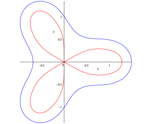
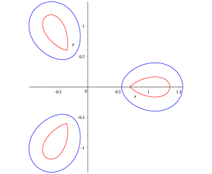
    accumulates on the level curves ๐’ž^rsubscript^๐’ž๐‘Ÿ\hat{\mathcal{C}}_{r} as in (1.22) with r=1๐‘Ÿ1r=1 for t<tc๐‘กsubscript๐‘ก๐‘t<t_{c} and r=tc2t2๐‘Ÿsuperscriptsubscript๐‘ก๐‘2superscript๐‘ก2r=\frac{t_{c}^{2}}{t^{2}} for t>tc๐‘กsubscript๐‘ก๐‘t>t_{c}. Namely the curve ๐’ž^^๐’ž\hat{\mathcal{C}} on which the zeros accumulate is given by

    ๐’ž^:|(tโˆ’ฮปs)exp(ฮปsโ€‹ttc2)|={tpre-critical caseย 0<t<tc,tc2tโ€‹et2tc2โˆ’1post-critical caseย t>tc,\hat{\mathcal{C}}:\quad\left|(t-\lambda^{s})\exp\left(\frac{\lambda^{s}t}{t_{c}^{2}}\right)\right|=\left\{\begin{array}[]{ll}t&\quad\mbox{pre-critical case $0<t<t_{c}$},\\ &\\ \dfrac{t_{c}^{2}}{t}e^{\frac{t^{2}}{t_{c}^{2}}-1}&\quad\mbox{post-critical case $t>t_{c}$},\end{array}\right. (1.25)

    with |ฮปsโˆ’t|โ‰คz0โ€‹tsuperscript๐œ†๐‘ ๐‘กsubscript๐‘ง0๐‘ก|\lambda^{s}-t|\leq z_{0}t. The measure ฮฝ^^๐œˆ\hat{\nu} in (1.23) is the weak-star limit of the normalized zero counting measure ฮฝnsubscript๐œˆ๐‘›\nu_{n} of the polynomials pnsubscript๐‘๐‘›p_{n} for n=sโ€‹k+l๐‘›๐‘ ๐‘˜๐‘™n=sk+l, l=0,โ€ฆ,sโˆ’2๐‘™0โ€ฆ๐‘ 2l=0,\dots,s-2.

Refer to caption
Refer to caption
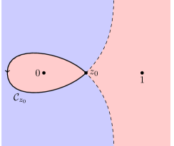
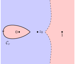
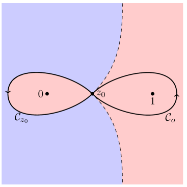
Figure 1.1: The blue contour is the boundary of the eigenvalue distribution support D๐ทD defined in (1.12) relative to the normal matrix model and the red contour is ๐’ž^^๐’ž\hat{\mathcal{C}} defined in (1.25) which describes the support of the limiting zero distribution of the polynomials pnโ€‹(ฮป)subscript๐‘๐‘›๐œ†p_{n}(\lambda). Here s=3๐‘ 3s=3 and t<tc๐‘กsubscript๐‘ก๐‘t<t_{c} (left figure) and t>tc๐‘กsubscript๐‘ก๐‘t>t_{c} (right figure).
Remark 1.5.

We observe that the curve (1.25) in the rescaled variable z=1โˆ’ฮปs/t๐‘ง1superscript๐œ†๐‘ ๐‘กz=1-\lambda^{s}/t takes the form

๐’ž:|ze1โˆ’zz0|={1pre-critical caseย z0>1,z0โ€‹e1z0โˆ’1post-critical caseย 0<z0<1.\mathcal{C}:\quad\left|ze^{\frac{1-z}{z_{0}}}\right|=\left\{\begin{array}[]{ll}1&\quad\mbox{pre-critical case $z_{0}>1$},\\ &\\ z_{0}e^{\frac{1}{z_{0}}-1}&\quad\mbox{post-critical case $0<z_{0}<1$}.\end{array}\right. (1.26)

with z0=tc2t2subscript๐‘ง0superscriptsubscript๐‘ก๐‘2superscript๐‘ก2z_{0}=\dfrac{t_{c}^{2}}{t^{2}} and |z|โ‰คz0๐‘งsubscript๐‘ง0|z|\leq z_{0}. The curve ๐’ž๐’ž\mathcal{C} is similar to the Szegล‘ curve {zโˆˆโ„‚:|zโ€‹e1โˆ’z|=1,|z|โ‰ค1}conditional-set๐‘งโ„‚formulae-sequence๐‘งsuperscript๐‘’1๐‘ง1๐‘ง1\{z\in\mathbb{C}\ \colon\ |ze^{1-z}|=1,\;\;|z|\leq 1\} that was first observed in relation to the zeros of the Taylor polynomials of the exponential function [52], and coincides exactly with such curve in the critical case z0=1subscript๐‘ง01z_{0}=1. The Szegรถ curve also appeared in the asymptotic analysis of the generalized Laguerre polynomials, see e.g.ย [45],[13],[40]. The curve (1.26) is the limiting curve for the zeros of the polynomials

ฯ€kโ€‹(z):=(โˆ’1)ktkโ€‹qk(l)โ€‹(โˆ’tโ€‹(zโˆ’1))assignsubscript๐œ‹๐‘˜๐‘งsuperscript1๐‘˜superscript๐‘ก๐‘˜subscriptsuperscript๐‘ž๐‘™๐‘˜๐‘ก๐‘ง1\pi_{k}(z):=\frac{(-1)^{k}}{t^{k}}q^{(l)}_{k}(-t(z-1)) (1.27)

where qk(l)โ€‹(u)subscriptsuperscript๐‘ž๐‘™๐‘˜๐‘ขq^{(l)}_{k}(u) have been defined in (1.17).

From Theoremย 1.4 and (1.8), the following identity follows immediately.

Lemma 1.6.

Given the potential Wโ€‹(ฮป)๐‘Š๐œ†W(\lambda) in (1.9), the measure ฮฝ^^๐œˆ\hat{\nu} in (1.23) with r=1๐‘Ÿ1r=1 for t<tc๐‘กsubscript๐‘ก๐‘t<t_{c} and r=tc2t2๐‘Ÿsuperscriptsubscript๐‘ก๐‘2superscript๐‘ก2r=\frac{t_{c}^{2}}{t^{2}} for t>tc๐‘กsubscript๐‘ก๐‘t>t_{c}, and the contour ๐’ž^^๐’ž\hat{\mathcal{C}} defined in (1.25), the equation

1Tโ€‹โˆ‚โˆ‚ฮปโ€‹Wโ€‹(ฮป)=โˆซ๐’ž^dโ€‹ฮฝ^โ€‹(ฮท)ฮปโˆ’ฮท,ฮปโˆ‰๐’ž^,formulae-sequence1๐‘‡๐œ†๐‘Š๐œ†subscript^๐’ž๐‘‘^๐œˆ๐œ‚๐œ†๐œ‚๐œ†^๐’ž\dfrac{1}{T}\dfrac{\partial}{\partial\lambda}W(\lambda)=\int_{\hat{\mathcal{C}}}\dfrac{d\hat{\nu}(\eta)}{\lambda-\eta},\quad\lambda\notin\hat{\mathcal{C}}, (1.28)

defines the boundary of a domain which coincides with D๐ทD defined in (1.12). The measure ฮผโˆ—superscript๐œ‡\mu^{*} in (1.11) of the eigenvalue distribution of the normal matrix model and the measure ฮฝ^^๐œˆ\hat{\nu} of the zero distribution of the orthogonal polynomials are related by

โˆซDdโ€‹ฮผโˆ—โ€‹(ฮท)ฮปโˆ’ฮท=โˆซ๐’ž^dโ€‹ฮฝ^โ€‹(ฮท)ฮปโˆ’ฮท,ฮปโˆˆโ„‚\D.formulae-sequencesubscript๐ท๐‘‘superscript๐œ‡๐œ‚๐œ†๐œ‚subscript^๐’ž๐‘‘^๐œˆ๐œ‚๐œ†๐œ‚๐œ†\โ„‚๐ท\int_{D}\dfrac{d\mu^{*}(\eta)}{\lambda-\eta}=\int_{\hat{\mathcal{C}}}\dfrac{d\hat{\nu}(\eta)}{\lambda-\eta},\quad\lambda\in\mathbb{C}\backslash D. (1.29)
Remark 1.7.

The identities (1.28) and (1.29) in Lemmaย 1.6 are expected to hold in general for a large class of normal matrix models. It has been verified for several other potentials (see, for example [2, 24, 6, 11, 38]).

We also observe that for the orthogonal polynomials appearing in random matrices, in some cases, the asymptotic distribution of the zeros is supported on the so-called mother body or potential theoretic skeleton of the support D๐ทD of the eigenvalue distribution. We recall that a measure ฮฝ๐œˆ\nu is a strong mother body for a domain D๐ทD with respect to a measure ฮผ๐œ‡\mu if [34]

  • 1)

    โˆซlogโก|ฮปโˆ’ฮท|โ€‹dโ€‹ฮผโ€‹(ฮท)โ‰คโˆซlogโก|ฮปโˆ’ฮท|โ€‹dโ€‹ฮฝโ€‹(ฮท)๐œ†๐œ‚๐‘‘๐œ‡๐œ‚๐œ†๐œ‚๐‘‘๐œˆ๐œ‚\int\log|\lambda-\eta|d\mu(\eta)\leq\int\log|\lambda-\eta|d\nu(\eta), for ฮปโˆˆโ„‚๐œ†โ„‚\lambda\in\mathbb{C} with equality for ฮป๐œ†\lambda outside D๐ทD;

  • 2)

    ฮฝโ‰ฅ0๐œˆ0\nu\geq 0 and suppย โ€‹ฮฝโŠ‚suppย โ€‹ฮผsuppย ๐œˆsuppย ๐œ‡\mbox{supp }\nu\subset\mbox{supp }\mu;

  • 3)

    the support of ฮฝ๐œˆ\nu has zero area measure;

  • 4)

    the support of ฮฝ๐œˆ\nu does not disconnect any part of D๐ทD from Dยฏcsuperscriptยฏ๐ท๐‘\bar{D}^{c}.

If the measure ฮฝ๐œˆ\nu has only the property 1), 2) and 3) it is called weak mother body. The problem of constructing mother bodies is not always solvable and the solution is not always unique [50].

Concerning the explicit examples appearing in the random matrix literature, for the exponential weight Wโ€‹(ฮป)=|ฮป|2+Reโก(Pโ€‹(ฮป))๐‘Š๐œ†superscript๐œ†2Re๐‘ƒ๐œ†W(\lambda)=|\lambda|^{2}+\operatorname{Re}(P(\lambda)) where Pโ€‹(ฮป)๐‘ƒ๐œ†P(\lambda) is polynomial, the support of the zero distribution of the orthogonal polynomials is a strong mother body of the domain that corresponds to the eigenvalue distribution of the matrix model (see, e.g., [11, 38, 31, 25, 54]). In contrast, in the model studied in [6] and also in the present case, the support of the zero distribution of the orthogonal polynomials does not have property 4) and therefore it is a weak mother body of the set D๐ทD.

The proof of Theoremย 1.4 is obtained from the strong and uniform asymptotics of the polynomials pnโ€‹(ฮป)subscript๐‘๐‘›๐œ†p_{n}(\lambda) in the whole complex plane which is obtained by characterising the orthogonal polynomials pnโ€‹(ฮป)subscript๐‘๐‘›๐œ†p_{n}(\lambda) via a Riemann-Hilbert method.
Uniform Asymptotics. In the next theorem we describe the strong and uniform asymptotic of the polynomials pnโ€‹(ฮป)subscript๐‘๐‘›๐œ†p_{n}(\lambda) in the complex plane. We distinguish the pre-critical case t<tc๐‘กsubscript๐‘ก๐‘t<t_{c} and post-critical case t>tc๐‘กsubscript๐‘ก๐‘t>t_{c}. We first define the function

ฯ•^โ€‹(ฮป)={ฯ•^r=z0โ€‹(ฮป)0<t<tc(pre-critical)ฯ•^r=1โ€‹(ฮป)tc<t(post-critical),^italic-ฯ•๐œ†casessubscript^italic-ฯ•๐‘Ÿsubscript๐‘ง0๐œ†0๐‘กsubscript๐‘ก๐‘(pre-critical)missing-subexpressionmissing-subexpressionmissing-subexpressionsubscript^italic-ฯ•๐‘Ÿ1๐œ†subscript๐‘ก๐‘๐‘ก(post-critical)\hat{\phi}(\lambda)=\left\{\begin{array}[]{lll}\hat{\phi}_{r=z_{0}}(\lambda)&0<t<t_{c}&\text{(pre-critical)}\\ &&\\ \hat{\phi}_{r=1}(\lambda)&t_{c}<t&\text{(post-critical)},\end{array}\right. (1.30)

where ฯ•^rโ€‹(ฮป)subscript^italic-ฯ•๐‘Ÿ๐œ†\hat{\phi}_{r}(\lambda) is given by (1.21).

Theorem 1.8 (Pre-critical case).

For 0<t<tc0๐‘กsubscript๐‘ก๐‘0<t<t_{c} the polynomial pnโ€‹(ฮป)subscript๐‘๐‘›๐œ†p_{n}(\lambda) with n=kโ€‹s+l๐‘›๐‘˜๐‘ ๐‘™n=ks+l, l=0,โ€ฆ,sโˆ’2๐‘™0โ€ฆ๐‘ 2l=0,\dots,s-2, ฮณ=sโˆ’lโˆ’1sโˆˆ(0,1)๐›พ๐‘ ๐‘™1๐‘ 01\gamma=\frac{s-l-1}{s}\in(0,1), have the following asymptotic behaviour for when n,Nโ†’โˆžโ†’๐‘›๐‘n,N\to\infty in such a way that Nโ€‹T=nโˆ’l๐‘๐‘‡๐‘›๐‘™NT=n-l:

  • (1)

    for ฮป๐œ†\lambda in compact subsets of the exterior of ๐’ž^^๐’ž\hat{\mathcal{C}} one has for any integer Mโ‰ฅ2๐‘€2M\geq 2

    pnโ€‹(ฮป)=ฮปsโˆ’1โ€‹(ฮปsโˆ’t)kโˆ’ฮณโ€‹(1+๐’ชโ€‹(1kM+ฮณ));subscript๐‘๐‘›๐œ†superscript๐œ†๐‘ 1superscriptsuperscript๐œ†๐‘ ๐‘ก๐‘˜๐›พ1๐’ช1superscript๐‘˜๐‘€๐›พp_{n}(\lambda)=\lambda^{s-1}(\lambda^{s}-t)^{k-\gamma}\left(1+{\mathcal{O}}\left(\frac{1}{k^{M+\gamma}}\right)\right); (1.31)
  • (2)

    for ฮป๐œ†\lambda near ๐’ž^^๐’ž\hat{\mathcal{C}} and away from ฮป=0๐œ†0\lambda=0,

    pnโ€‹(ฮป)=ฮปsโˆ’1โ€‹(ฮปsโˆ’t)kโˆ’ฮณโ€‹[1+eโˆ’kโ€‹ฯ•^โ€‹(ฮป)k1+ฮณโ€‹(1ฮ“โ€‹(โˆ’ฮณ)โ€‹(1โˆ’1z0)โˆ’1โˆ’ฮณโ€‹tฮปsโ€‹(1โˆ’tฮปs)ฮณ+๐’ชโ€‹(1k))],subscript๐‘๐‘›๐œ†superscript๐œ†๐‘ 1superscriptsuperscript๐œ†๐‘ ๐‘ก๐‘˜๐›พdelimited-[]1superscript๐‘’๐‘˜^italic-ฯ•๐œ†superscript๐‘˜1๐›พ1ฮ“๐›พsuperscript11subscript๐‘ง01๐›พ๐‘กsuperscript๐œ†๐‘ superscript1๐‘กsuperscript๐œ†๐‘ ๐›พ๐’ช1๐‘˜p_{n}(\lambda)=\lambda^{s-1}(\lambda^{s}-t)^{k-\gamma}\left[1+\dfrac{e^{-k\hat{\phi}(\lambda)}}{k^{1+\gamma}}\left(\dfrac{1}{\Gamma(-\gamma)}\left(1-\frac{1}{z_{0}}\right)^{-1-\gamma}\dfrac{t}{\lambda^{s}}\left(1-\frac{t}{\lambda^{s}}\right)^{\gamma}+{\mathcal{O}}\left(\frac{1}{k}\right)\right)\right]\,, (1.32)

    where ฯ•^โ€‹(ฮป)^italic-ฯ•๐œ†\hat{\phi}(\lambda) has been defined in (1.30) and ฮ“โ€‹(z)=(zโˆ’1)!ฮ“๐‘ง๐‘ง1\Gamma(z)=(z-1)!;

  • (3)

    for ฮป๐œ†\lambda in compact subsets of the interior of ๐’ž^^๐’ž\hat{\mathcal{C}} and away from ฮป=0๐œ†0\lambda=0,

    pnโ€‹(ฮป)=ฮปlโ€‹eโˆ’kโ€‹ฮปstโ€‹z0k1+ฮณโ€‹((โˆ’t)k+1ฮ“โ€‹(โˆ’ฮณ)โ€‹1ฮปsโ€‹(1โˆ’1z0)โˆ’1โˆ’ฮณ+๐’ชโ€‹(1k));subscript๐‘๐‘›๐œ†superscript๐œ†๐‘™superscript๐‘’๐‘˜superscript๐œ†๐‘ ๐‘กsubscript๐‘ง0superscript๐‘˜1๐›พsuperscript๐‘ก๐‘˜1ฮ“๐›พ1superscript๐œ†๐‘ superscript11subscript๐‘ง01๐›พ๐’ช1๐‘˜p_{n}(\lambda)=\lambda^{l}\dfrac{e^{-\frac{k\lambda^{s}}{tz_{0}}}}{k^{1+\gamma}}\left(\dfrac{(-t)^{k+1}}{\Gamma(-\gamma)}\dfrac{1}{\lambda^{s}}\left(1-\frac{1}{z_{0}}\right)^{-1-\gamma}+{\mathcal{O}}\left(\frac{1}{k}\right)\right); (1.33)
  • (4)

    for ฮป๐œ†\lambda in a neighbourhood of ฮป=0๐œ†0\lambda=0, we introduce the function w^โ€‹(ฮป)=ฯ•^โ€‹(ฮป)+2โ€‹ฯ€โ€‹i^๐‘ค๐œ†^italic-ฯ•๐œ†2๐œ‹๐‘–\hat{w}(\lambda)=\hat{\phi}(\lambda)+2\pi i if ฮปsโˆˆโ„‚โˆ’superscript๐œ†๐‘ subscriptโ„‚\lambda^{s}\in\mathbb{C}_{-} and w^โ€‹(ฮป)=ฯ•^โ€‹(ฮป)^๐‘ค๐œ†^italic-ฯ•๐œ†\hat{w}(\lambda)=\hat{\phi}(\lambda) if ฮปsโˆˆโ„‚+superscript๐œ†๐‘ subscriptโ„‚\lambda^{s}\in\mathbb{C}_{+}. Then

    pnโ€‹(ฮป)=ฮปlโ€‹(ฮปsโˆ’t)kโˆ’ฮณโ€‹(ฮปsw^โ€‹(ฮป))ฮณโ€‹[(w^โ€‹(ฮป))ฮณโˆ’eโˆ’kโ€‹ฯ•^โ€‹(ฮป)kฮณโ€‹(ฮจ~12โ€‹(kโ€‹w^โ€‹(ฮป))+๐’ชโ€‹(1k))],subscript๐‘๐‘›๐œ†superscript๐œ†๐‘™superscriptsuperscript๐œ†๐‘ ๐‘ก๐‘˜๐›พsuperscriptsuperscript๐œ†๐‘ ^๐‘ค๐œ†๐›พdelimited-[]superscript^๐‘ค๐œ†๐›พsuperscript๐‘’๐‘˜^italic-ฯ•๐œ†superscript๐‘˜๐›พsubscript~ฮจ12๐‘˜^๐‘ค๐œ†๐’ช1๐‘˜p_{n}(\lambda)=\lambda^{l}(\lambda^{s}-t)^{k-\gamma}\left(\dfrac{\lambda^{s}}{\hat{w}(\lambda)}\right)^{\gamma}\left[(\hat{w}(\lambda))^{\gamma}-\dfrac{e^{-k\hat{\phi}(\lambda)}}{k^{\gamma}}\left(\tilde{\Psi}_{12}(k\hat{w}(\lambda))+{\mathcal{O}}\left(\frac{1}{k}\right)\right)\right], (1.34)

where the (1,2)12(1,2)-entry of the matrix ฮจ~~ฮจ\tilde{\Psi} is defined in (3.52).

We observe that in compact subsets of the exterior of ๐’ž^^๐’ž\hat{\mathcal{C}} there are no zeros of the polynomials pnโ€‹(ฮป)subscript๐‘๐‘›๐œ†p_{n}(\lambda). The only possible zeros are located in ฮป=0๐œ†0\lambda=0 and in the region where the second term in parenthesis in the expression (1.32) is of order one. Since Reโกฯ•^โ€‹(ฮป)Re^italic-ฯ•๐œ†\operatorname{Re}\hat{\phi}(\lambda) is negative inside ๐’ž^^๐’ž\hat{\mathcal{C}} and positive outside ๐’ž^^๐’ž\hat{\mathcal{C}} it follows that the possible zeros of pnโ€‹(ฮป)subscript๐‘๐‘›๐œ†p_{n}(\lambda) lie inside ๐’ž^^๐’ž\hat{\mathcal{C}} and are determined by the condition

Reโกฯ•^โ€‹(ฮป)=โˆ’(1+ฮณ)โ€‹logโกkk+1kโ€‹logโก(1|ฮ“โ€‹(โˆ’ฮณ)|โ€‹t|ฮป|sโ€‹|1โˆ’1z0|โˆ’1โˆ’ฮณโ€‹|1โˆ’tฮปs|ฮณ),|ฮปsโˆ’t|โ‰คt.formulae-sequenceRe^italic-ฯ•๐œ†1๐›พ๐‘˜๐‘˜1๐‘˜1ฮ“๐›พ๐‘กsuperscript๐œ†๐‘ superscript11subscript๐‘ง01๐›พsuperscript1๐‘กsuperscript๐œ†๐‘ ๐›พsuperscript๐œ†๐‘ ๐‘ก๐‘ก\operatorname{Re}\hat{\phi}(\lambda)=-(1+\gamma)\dfrac{\log k}{k}+\dfrac{1}{k}\log\left(\dfrac{1}{|\Gamma(-\gamma)|}\dfrac{t}{|\lambda|^{s}}\left|1-\frac{1}{z_{0}}\right|^{-1-\gamma}\left|1-\frac{t}{\lambda^{s}}\right|^{\gamma}\right),\quad|\lambda^{s}-t|\leq t. (1.35)

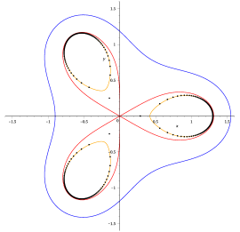
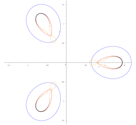
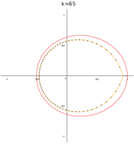
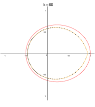
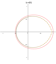
The expansion (1.32) shows that the zeros of the polynomials pnโ€‹(ฮป)subscript๐‘๐‘›๐œ†p_{n}(\lambda) are within a distance ๐’ชโ€‹(1/k2)๐’ช1superscript๐‘˜2{\mathcal{O}}\left(1/k^{2}\right) from the level curve (1.35). This level curve approaches ๐’ž^^๐’ž\hat{\mathcal{C}} defined in (1.25) at a rate ๐’ชโ€‹(logโกk/k)๐’ช๐‘˜๐‘˜{\mathcal{O}}\left(\log k/k\right).

Refer to caption
Refer to caption
Figure 1.2: The blue contour is the boundary of the support of the eigenvalue distribution defined in (1.12) and the red contour ๐’ž^^๐’ž\hat{\mathcal{C}} defined in (1.25), is the support of the limiting zero distribution of the orthogonal polynomials pnโ€‹(ฮป)subscript๐‘๐‘›๐œ†p_{n}(\lambda). The yellow contour is given by (1.35) in the pre-critical case and (1.40) in the post-critical case and lies within a distance of order ๐’ชโ€‹(logโกnn)๐’ช๐‘›๐‘›{\mathcal{O}}\left(\frac{\log n}{n}\right) from the contour ๐’ž^^๐’ž\hat{\mathcal{C}}. The dots are the zeros of the polynomial pnโ€‹(ฮป)subscript๐‘๐‘›๐œ†p_{n}(\lambda) for s=3๐‘ 3s=3, n=285๐‘›285n=285, l=0๐‘™0l=0 and t<tc๐‘กsubscript๐‘ก๐‘t<t_{c} on the right and t>tc๐‘กsubscript๐‘ก๐‘t>t_{c} on the left, respectively.

For t>tc๐‘กsubscript๐‘ก๐‘t>t_{c} the polynomials pnโ€‹(ฮป)subscript๐‘๐‘›๐œ†p_{n}(\lambda) with n=kโ€‹s+l๐‘›๐‘˜๐‘ ๐‘™n=ks+l, l=0,โ€ฆ,sโˆ’2๐‘™0โ€ฆ๐‘ 2l=0,\dots,s-2, have the following asymptotic behaviour.

Theorem 1.9 (Post-critical case).

For t>tc๐‘กsubscript๐‘ก๐‘t>t_{c} the polynomials pnโ€‹(ฮป)subscript๐‘๐‘›๐œ†p_{n}(\lambda) with n=kโ€‹s+l๐‘›๐‘˜๐‘ ๐‘™n=ks+l, l=0,โ€ฆ,sโˆ’2๐‘™0โ€ฆ๐‘ 2l=0,\dots,s-2, and ฮณ=sโˆ’lโˆ’1sโˆˆ(0,1)๐›พ๐‘ ๐‘™1๐‘ 01\gamma=\frac{s-l-1}{s}\in(0,1) have the following behaviour when n,Nโ†’โˆžโ†’๐‘›๐‘n,N\to\infty in such a way that Nโ€‹T=nโˆ’l๐‘๐‘‡๐‘›๐‘™NT=n-l

  • (1)

    for ฮป๐œ†\lambda in compact subsets of the exterior of ๐’ž^^๐’ž\hat{\mathcal{C}} one has

    pnโ€‹(ฮป)=ฮปlโ€‹(ฮปsโˆ’t)kโˆ’ฮณโ€‹(ฮปs+tโ€‹(z0โˆ’1))ฮณโ€‹(1+๐’ชโ€‹(1k)),subscript๐‘๐‘›๐œ†superscript๐œ†๐‘™superscriptsuperscript๐œ†๐‘ ๐‘ก๐‘˜๐›พsuperscriptsuperscript๐œ†๐‘ ๐‘กsubscript๐‘ง01๐›พ1๐’ช1๐‘˜p_{n}(\lambda)=\lambda^{l}(\lambda^{s}-t)^{k-\gamma}(\lambda^{s}+t(z_{0}-1))^{\gamma}\left(1+{\mathcal{O}}\left(\frac{1}{k}\right)\right), (1.36)

    with z0=tc2t2subscript๐‘ง0superscriptsubscript๐‘ก๐‘2superscript๐‘ก2z_{0}=\dfrac{t_{c}^{2}}{t^{2}};

  • (2)

    for ฮป๐œ†\lambda in the region near ๐’ž^^๐’ž\hat{\mathcal{C}} and away from the points ฮปs=tโ€‹(1โˆ’z0)superscript๐œ†๐‘ ๐‘ก1subscript๐‘ง0\lambda^{s}=t(1-z_{0}) one has

    pnโ€‹(ฮป)=ฮปlโ€‹(ฮปsโˆ’t)kโˆ’ฮณโ€‹(ฮปs+tโ€‹(z0โˆ’1))ฮณโ€‹(1โˆ’eโˆ’kโ€‹ฯ•^โ€‹(ฮป)k12+ฮณโ€‹ฮณโ€‹z02cโ€‹tโ€‹((ฮปsโˆ’t)โ€‹ฮปs)ฮณ(ฮปs+tโ€‹(z0โˆ’1))2โ€‹ฮณ+1+๐’ชโ€‹(1k)),subscript๐‘๐‘›๐œ†superscript๐œ†๐‘™superscriptsuperscript๐œ†๐‘ ๐‘ก๐‘˜๐›พsuperscriptsuperscript๐œ†๐‘ ๐‘กsubscript๐‘ง01๐›พ1superscript๐‘’๐‘˜^italic-ฯ•๐œ†superscript๐‘˜12๐›พ๐›พsuperscriptsubscript๐‘ง02๐‘๐‘กsuperscriptsuperscript๐œ†๐‘ ๐‘กsuperscript๐œ†๐‘ ๐›พsuperscriptsuperscript๐œ†๐‘ ๐‘กsubscript๐‘ง012๐›พ1๐’ช1๐‘˜p_{n}(\lambda)=\lambda^{l}(\lambda^{s}-t)^{k-\gamma}(\lambda^{s}+t(z_{0}-1))^{\gamma}\left(1-\dfrac{e^{-k\hat{\phi}(\lambda)}}{k^{\frac{1}{2}+\gamma}}\dfrac{\gamma z_{0}^{2}}{c}\dfrac{t((\lambda^{s}-t)\lambda^{s})^{\gamma}}{(\lambda^{s}+t(z_{0}-1))^{2\gamma+1}}+{\mathcal{O}}\left(\frac{1}{k}\right)\right), (1.37)

    with ฯ•^โ€‹(ฮป)^italic-ฯ•๐œ†\hat{\phi}(\lambda) defined in (1.30) and the constant c๐‘c defined in (4.54);

  • (3)

    for ฮป๐œ†\lambda in compact subsets of the interior region of ๐’ž^^๐’ž\hat{\mathcal{C}} one has

    pnโ€‹(ฮป)=ฮปlโ€‹ekโ€‹tโˆ’ฮปstโ€‹z0k12+ฮณโ€‹tโ€‹ฮณโ€‹z02cโ€‹(tโ€‹z0e)kโ€‹(ฮปsโ€‹ฮณ(ฮปs+tโ€‹(z0โˆ’1))ฮณ+1+๐’ชโ€‹(1k));subscript๐‘๐‘›๐œ†superscript๐œ†๐‘™superscript๐‘’๐‘˜๐‘กsuperscript๐œ†๐‘ ๐‘กsubscript๐‘ง0superscript๐‘˜12๐›พ๐‘ก๐›พsuperscriptsubscript๐‘ง02๐‘superscript๐‘กsubscript๐‘ง0๐‘’๐‘˜superscript๐œ†๐‘ ๐›พsuperscriptsuperscript๐œ†๐‘ ๐‘กsubscript๐‘ง01๐›พ1๐’ช1๐‘˜p_{n}(\lambda)=\lambda^{l}\dfrac{e^{k\frac{t-\lambda^{s}}{tz_{0}}}}{k^{\frac{1}{2}+\gamma}}\dfrac{t\gamma z_{0}^{2}}{c}\left(\dfrac{tz_{0}}{e}\right)^{k}\left(\dfrac{\lambda^{s\gamma}}{(\lambda^{s}+t(z_{0}-1))^{\gamma+1}}+{\mathcal{O}}\left(\frac{1}{k}\right)\right); (1.38)
  • (4)

    in the neighbourhood of each of the points that solve the equation ฮปs=tโ€‹(1โˆ’z0)superscript๐œ†๐‘ ๐‘ก1subscript๐‘ง0\lambda^{s}=t(1-z_{0}) one has

    pnโ€‹(ฮป)=ฮปlโ€‹(ฮปsโˆ’t)kโˆ’ฮณโ€‹(ฮปs+tโ€‹(z0โˆ’1)kโ€‹w^โ€‹(ฮป))ฮณโ€‹eโˆ’kโ€‹ฯ•^โ€‹(ฮป)โ€‹(๐’ฐโ€‹(โˆ’ฮณโˆ’12;2โ€‹kโ€‹w^โ€‹(ฮป))+๐’ชโ€‹(1k));subscript๐‘๐‘›๐œ†superscript๐œ†๐‘™superscriptsuperscript๐œ†๐‘ ๐‘ก๐‘˜๐›พsuperscriptsuperscript๐œ†๐‘ ๐‘กsubscript๐‘ง01๐‘˜^๐‘ค๐œ†๐›พsuperscript๐‘’๐‘˜^italic-ฯ•๐œ†๐’ฐ๐›พ122๐‘˜^๐‘ค๐œ†๐’ช1๐‘˜p_{n}(\lambda)=\lambda^{l}(\lambda^{s}-t)^{k-\gamma}\left(\dfrac{\lambda^{s}+t(z_{0}-1)}{\sqrt{k}\hat{w}(\lambda)}\right)^{\gamma}e^{-k\hat{\phi}(\lambda)}\left({\cal U}(-\gamma-\frac{1}{2};\sqrt{2k}\hat{w}(\lambda))+{\mathcal{O}}\left(\frac{1}{k}\right)\right); (1.39)

    where ๐’ฐโ€‹(a;ฮพ)๐’ฐ๐‘Ž๐œ‰{\cal U}(a;\xi) is the parabolic cylinder function (Chap.ย 13, [1]) satisfying the equation d2dโ€‹ฮพ2โ€‹๐’ฐ=(14โ€‹ฮพ2+a)โ€‹๐’ฐsuperscript๐‘‘2๐‘‘superscript๐œ‰2๐’ฐ14superscript๐œ‰2๐‘Ž๐’ฐ\dfrac{d^{2}}{d\xi^{2}}{\cal U}=\left(\frac{1}{4}\xi^{2}+a\right){\cal U} and w^2โ€‹(ฮป)=โˆ’ฯ•^โ€‹(ฮป)โˆ’2โ€‹ฯ€โ€‹isuperscript^๐‘ค2๐œ†^italic-ฯ•๐œ†2๐œ‹๐‘–\hat{w}^{2}(\lambda)=-\hat{\phi}(\lambda)-2\pi i for ฮปsโˆˆโ„‚โˆ’superscript๐œ†๐‘ subscriptโ„‚\lambda^{s}\in\mathbb{C}_{-} and w^2โ€‹(ฮป)=โˆ’ฯ•^โ€‹(ฮป)superscript^๐‘ค2๐œ†^italic-ฯ•๐œ†\hat{w}^{2}(\lambda)=-\hat{\phi}(\lambda) for ฮปsโˆˆโ„‚+superscript๐œ†๐‘ subscriptโ„‚\lambda^{s}\in\mathbb{C}_{+}.

We observe that in compact subsets of the exterior of ๐’ž^^๐’ž\hat{\mathcal{C}} the polynomials pnโ€‹(ฮป)subscript๐‘๐‘›๐œ†p_{n}(\lambda) have zero at ฮป=0๐œ†0\lambda=0 with multiplicity l๐‘™l. The other possible zeros are located in the region where the second term in parenthesis in the expression (1.37) is of order one. This happens in the region where Reโกฯ•^โ€‹(ฮป)<0Re^italic-ฯ•๐œ†0\operatorname{Re}\hat{\phi}(\lambda)<0 and Reโกฯ•^โ€‹(ฮป)=๐’ชโ€‹(logโกk/k)Re^italic-ฯ•๐œ†๐’ช๐‘˜๐‘˜\operatorname{Re}\hat{\phi}(\lambda)={\mathcal{O}}\left(\log k/k\right), namely in a region inside the contour ๐’ž^^๐’ž\hat{\mathcal{C}} and defined by the equation

Reโกฯ•^โ€‹(ฮป)=โˆ’(1+ฮณ)โ€‹logโกkk+1kโ€‹logโก(tโ€‹ฮณโ€‹z02|c|โ€‹|(ฮปsโˆ’t)โ€‹ฮปs|ฮณ|ฮปs+tโ€‹(z0โˆ’1)|2โ€‹ฮณ+1).Re^italic-ฯ•๐œ†1๐›พ๐‘˜๐‘˜1๐‘˜๐‘ก๐›พsuperscriptsubscript๐‘ง02๐‘superscriptsuperscript๐œ†๐‘ ๐‘กsuperscript๐œ†๐‘ ๐›พsuperscriptsuperscript๐œ†๐‘ ๐‘กsubscript๐‘ง012๐›พ1\operatorname{Re}\hat{\phi}(\lambda)=-(1+\gamma)\dfrac{\log k}{k}+\dfrac{1}{k}\log\left(\dfrac{t\gamma z_{0}^{2}}{|c|}\dfrac{|(\lambda^{s}-t)\lambda^{s}|^{\gamma}}{|\lambda^{s}+t(z_{0}-1)|^{2\gamma+1}}\right). (1.40)

The expansion (1.37) shows that the zeros of the polynomials pnโ€‹(ฮป)subscript๐‘๐‘›๐œ†p_{n}(\lambda) are within a distance ๐’ชโ€‹(1/k2)๐’ช1superscript๐‘˜2{\mathcal{O}}\left(1/k^{2}\right)from the level curve (1.40). This level curve approaches ๐’ž^^๐’ž\hat{\mathcal{C}} defined in (1.25) at a rate ๐’ชโ€‹(logโกk/k)๐’ช๐‘˜๐‘˜{\mathcal{O}}\left(\log k/k\right).

The proofs of Theoremย 1.8 and Theoremย 1.9 are obtained by reducing the planar orthogonality relations of the polynomials pnโ€‹(ฮป)subscript๐‘๐‘›๐œ†p_{n}(\lambda) to orthogonality relations with respect to a complex density on a contour. More precisely, the sequence of polynomials pnโ€‹(ฮป)subscript๐‘๐‘›๐œ†p_{n}(\lambda) can be reduced to s๐‘ s families of polynomials qk(l)โ€‹(ฮปs)subscriptsuperscript๐‘ž๐‘™๐‘˜superscript๐œ†๐‘ q^{(l)}_{k}(\lambda^{s}), l=0,โ€ฆ,sโˆ’1๐‘™0โ€ฆ๐‘ 1l=0,\dots,s-1 as in (1.17) with n=kโ€‹s+l๐‘›๐‘˜๐‘ ๐‘™n=ks+l. The orthogonality relations of the polynomials q(l)โ€‹(u)superscript๐‘ž๐‘™๐‘ขq^{(l)}(u) are reduced to orthogonality relations on a contour. We then reformulate such orthogonality relation as a Riemann-Hilbert problem. We perform the asymptotic analysis of the polynomials qk(l)โ€‹(ฮป)subscriptsuperscript๐‘ž๐‘™๐‘˜๐œ†q^{(l)}_{k}(\lambda) using the nonlinear steepest descent/stationary phase method introduced by Deift and Zhou [22] and successfully applied in Hermitian random matrices and orthogonal polynomials on the line in the seminal papers, [19],[20]. See [21] for an introduction to this method, with a special emphasis on the applications to orthogonal polynomials and random matrices. It would be also interesting to explore the asymptotic for the polynomials pnโ€‹(ฮป)subscript๐‘๐‘›๐œ†p_{n}(\lambda) using the โˆ‚ยฏยฏ\bar{\partial}-problem introduced in [36].

The zeros of pnโ€‹(ฮป)subscript๐‘๐‘›๐œ†p_{n}(\lambda) accumulate along an open contour as shown in Figureย 1.1. The determination of this contour is a first step in the analysis. Riemannโ€“Hilbert analysis in which a contour selection method was required, also appeared in the papers [6],[40].

The Riemann-Hilbert method gives strong and uniform asymptotics of the polynomials pnโ€‹(ฮป)subscript๐‘๐‘›๐œ†p_{n}(\lambda) in the whole complex plane. The asymptotic behaviour of the polynomials pnโ€‹(ฮป)subscript๐‘๐‘›๐œ†p_{n}(\lambda) in the leading and sub-leading order can be expressed in terms of elementary functions in the pre-critical case t<tc๐‘กsubscript๐‘ก๐‘t<t_{c}, while in the post-critical case t>tc๐‘กsubscript๐‘ก๐‘t>t_{c} we have used, in some regions of the complex plane, parabolic cylinder functions as in [22],[37],[46]. The proof of Theoremย 1.4 is then deduced from the strong asymptotic of the orthogonal polynomials.

The paper is organized as follows:

  • โ€ข

    In Sect.ย 2, by using the symmetry properties of the external potential, we reduce the orthogonality relations of the polynomials pnโ€‹(ฮป)subscript๐‘๐‘›๐œ†p_{n}(\lambda) on a contour and recall how to formulate a Riemann-Hilbert problem for such orthogonal polynomials [27].

  • โ€ข

    In Sect.ย 3 we obtain the strong and uniform asymptotics for the polynomials pnโ€‹(ฮป)subscript๐‘๐‘›๐œ†p_{n}(\lambda) in the pre-critical case t<tc๐‘กsubscript๐‘ก๐‘t<t_{c}.

  • โ€ข

    In Sect.ย 4 we find the strong and uniform asymptotics for the polynomials pnโ€‹(ฮป)subscript๐‘๐‘›๐œ†p_{n}(\lambda) in the post-critical case t>tc๐‘กsubscript๐‘ก๐‘t>t_{c} and we prove Theoremย 1.4.

In the critical case t=tc๐‘กsubscript๐‘ก๐‘t=t_{c}, the set D๐ทD in (1.12) that supports the eigenvalue distribution of the normal matrix models has a singularity in ฮป=0๐œ†0\lambda=0. The corresponding asymptotics of the orthogonal polynomials seems to be described in terms of Painlevรฉ IV equation as in [17] and this situation is quite different from the generic singularity that have been described in terms of the Painlevรฉ I equation [41],[39]. Such problem will be investigated in a subsequent publication.

Furthermore, from the norming constants of the orthogonal polynomials, one may consider the problem of determining the asymptotic expansion of the partition function Zn,Nsubscript๐‘๐‘›๐‘Z_{n,N} in the spirit of [16]. Also this problem will be investigated in a subsequent publication.

Acknowledgements. The authors thank M.ย Bertola, G.ย Silva, A.ย Tovbis for useful discussions and K.ย McLaughin for suggesting the problem. The first part of this work was carried out while F.B.ย was a postdoctoral fellow at SISSA, later he was supported in part by the Fonds de recherche du Quรฉbec - Nature et technologies (FRQNT) via the research grant Matrices Alรฉatoires, Processus Stochastiques et Systรจmes Intรฉgrables. F.ย B.ย acknowledges the excellent working conditions at Concordia University and at the Centre des Recherches Mathรฉmatiques (CRM). T.ย G.ย acknowledges the support by the Leverhulme Trust Research Fellowship RF-2015-442 and the Miur Research project Geometric and analytic theory of Hamiltonian systems in finite and infinite dimensions of Italian Ministry of Universities and Research.

2 The associated Riemannโ€“Hilbert problem

In this section we set up the Riemannโ€“Hilbert problem to study the asymptotic behaviour of the orthogonal polynomials pnโ€‹(ฮป)subscript๐‘๐‘›๐œ†p_{n}(\lambda). As seen above, the analysis of pnโ€‹(ฮป)subscript๐‘๐‘›๐œ†p_{n}(\lambda) can be reduced to that of the polynomials qk(l)โ€‹(ฮปd)superscriptsubscript๐‘ž๐‘˜๐‘™superscript๐œ†๐‘‘q_{k}^{(l)}(\lambda^{d}) introduced in (1.17). The polynomials qk(l)โ€‹(u)superscriptsubscript๐‘ž๐‘˜๐‘™๐‘ขq_{k}^{(l)}(u) are characterized by the symmetry-reduced orthogonality relations

โˆซโ„‚qk(l)โ€‹(u)โ€‹uยฏjโ€‹|u|โˆ’2โ€‹ฮณโ€‹eโˆ’Nโ€‹(|u|2โˆ’tโ€‹uโˆ’tโ€‹uยฏ)โ€‹๐‘‘Aโ€‹(u)=0,j=0,โ€ฆ,kโˆ’1.formulae-sequencesubscriptโ„‚superscriptsubscript๐‘ž๐‘˜๐‘™๐‘ขsuperscriptยฏ๐‘ข๐‘—superscript๐‘ข2๐›พsuperscript๐‘’๐‘superscript๐‘ข2๐‘ก๐‘ข๐‘กยฏ๐‘ขdifferential-d๐ด๐‘ข0๐‘—0โ€ฆ๐‘˜1\int_{\mathbb{C}}q_{k}^{(l)}(u)\bar{u}^{j}|u|^{-2\gamma}e^{-N\left(|u|^{2}-tu-t\bar{u}\right)}dA(u)=0,\qquad j=0,\dots,k-1. (2.1)

2.1 Reduction to contour integral orthogonality

The crucial step in the present analysis is to replace the two-dimensional integral conditions (2.1) by an equivalent set of linear constraints in terms of contour integrals. In what follows it will be advantageous to perform the change of coordinate

u=โˆ’tโ€‹(zโˆ’1),zโˆˆโ„‚,formulae-sequence๐‘ข๐‘ก๐‘ง1๐‘งโ„‚u=-t(z-1),\quad z\in\mathbb{C}, (2.2)

and characterize qk(l)โ€‹(u)superscriptsubscript๐‘ž๐‘˜๐‘™๐‘ขq_{k}^{(l)}(u) in terms of the transformed polynomial

ฯ€kโ€‹(z):=(โˆ’1)ktkโ€‹qk(l)โ€‹(โˆ’tโ€‹(zโˆ’1))assignsubscript๐œ‹๐‘˜๐‘งsuperscript1๐‘˜superscript๐‘ก๐‘˜subscriptsuperscript๐‘ž๐‘™๐‘˜๐‘ก๐‘ง1\pi_{k}(z):=\frac{(-1)^{k}}{t^{k}}q^{(l)}_{k}(-t(z-1)) (2.3)

in the new variable z๐‘งz. The polynomial ฯ€kโ€‹(z)subscript๐œ‹๐‘˜๐‘ง\pi_{k}(z) is also a monic polynomial of degree k๐‘˜k and it can be characterized as follows.

Theorem 2.1.

The polynomial ฯ€kโ€‹(z)subscript๐œ‹๐‘˜๐‘ง\pi_{k}(z) is characterized by the non-hermitian orthogonality relations

โˆฎฮฃฯ€kโ€‹(z)โ€‹zjโ€‹eโˆ’Nโ€‹t2โ€‹zzkโ€‹(zzโˆ’1)ฮณโ€‹๐‘‘z=0j=0,1,โ€ฆ,kโˆ’1,ฮณโˆˆ(0,1),formulae-sequencesubscriptcontour-integralฮฃsubscript๐œ‹๐‘˜๐‘งsuperscript๐‘ง๐‘—superscript๐‘’๐‘superscript๐‘ก2๐‘งsuperscript๐‘ง๐‘˜superscript๐‘ง๐‘ง1๐›พdifferential-d๐‘ง0formulae-sequence๐‘—01โ€ฆ๐‘˜1๐›พ01\oint_{\Sigma}\pi_{k}(z)z^{j}\frac{e^{-Nt^{2}z}}{z^{k}}\left(\frac{z}{z-1}\right)^{\gamma}dz=0\qquad j=0,1,\dots,k-1\ ,\;\;\gamma\in(0,1), (2.4)

where ฮฃฮฃ\Sigma is a simple positively oriented contour encircling z=0๐‘ง0z=0 and z=1๐‘ง1z=1 and the function (zzโˆ’1)ฮณsuperscript๐‘ง๐‘ง1๐›พ\left(\frac{z}{z-1}\right)^{\gamma} is analytic in โ„‚\[0,1]\โ„‚01\mathbb{C}\backslash[0,1] and tends to one for |z|โ†’โˆžโ†’๐‘ง|z|\to\infty.

Refer to caption
Figure 2.1: The contour ฮฃฮฃ\Sigma

Proof.ย In order to prove the theorem we first show that the orthogonality relation for the polynomials qklโ€‹(u)subscriptsuperscript๐‘ž๐‘™๐‘˜๐‘ขq^{l}_{k}(u) on the plane can be reduced to an orthogonality relation on a contour. To this end we seek a function ฯ‡jโ€‹(u,uยฏ)subscript๐œ’๐‘—๐‘ขยฏ๐‘ข\chi_{j}(u,\bar{u}) that solves the โˆ‚ยฏยฏ\bar{\partial}-problem

โˆ‚uยฏฯ‡jโ€‹(u,uยฏ)=uยฏjโ€‹|u|โˆ’2โ€‹ฮณโ€‹eโˆ’Nโ€‹(|u|2โˆ’tโ€‹uโˆ’tโ€‹uยฏ).subscriptยฏ๐‘ขsubscript๐œ’๐‘—๐‘ขยฏ๐‘ขsuperscriptยฏ๐‘ข๐‘—superscript๐‘ข2๐›พsuperscript๐‘’๐‘superscript๐‘ข2๐‘ก๐‘ข๐‘กยฏ๐‘ข\partial_{\overline{u}}\chi_{j}(u,\bar{u})=\overline{u}^{j}|u|^{-2\gamma}e^{-N\left(|u|^{2}-tu-t\overline{u}\right)}. (2.5)

Having such a function, for any polynomial qโ€‹(u)๐‘ž๐‘ขq(u) one has

dโ€‹[qโ€‹(u)โ€‹ฯ‡jโ€‹(u,uยฏ)โ€‹dโ€‹u]๐‘‘delimited-[]๐‘ž๐‘ขsubscript๐œ’๐‘—๐‘ขยฏ๐‘ข๐‘‘๐‘ข\displaystyle d\left[q(u)\chi_{j}(u,\overline{u})du\right] =qโ€‹(u)โ€‹โˆ‚uยฏฯ‡jโ€‹(u,uยฏ)โ€‹dโ€‹uยฏโˆงdโ€‹uabsent๐‘ž๐‘ขsubscriptยฏ๐‘ขsubscript๐œ’๐‘—๐‘ขยฏ๐‘ข๐‘‘ยฏ๐‘ข๐‘‘๐‘ข\displaystyle=q(u)\partial_{\overline{u}}\chi_{j}(u,\overline{u})d\overline{u}\wedge du (2.6)
=qโ€‹(u)โ€‹uยฏjโ€‹|u|โˆ’2โ€‹ฮณโ€‹eโˆ’Nโ€‹(|u|2โˆ’tโ€‹uโˆ’tโ€‹uยฏ)โ€‹dโ€‹uยฏโˆงdโ€‹u,absent๐‘ž๐‘ขsuperscriptยฏ๐‘ข๐‘—superscript๐‘ข2๐›พsuperscript๐‘’๐‘superscript๐‘ข2๐‘ก๐‘ข๐‘กยฏ๐‘ข๐‘‘ยฏ๐‘ข๐‘‘๐‘ข\displaystyle=q(u)\overline{u}^{j}|u|^{-2\gamma}e^{-N\left(|u|^{2}-tu-t\overline{u}\right)}d\overline{u}\wedge du, (2.7)

where d๐‘‘d denotes the operation of exterior differentiation. If such ฯ‡jโ€‹(u,uยฏ)subscript๐œ’๐‘—๐‘ขยฏ๐‘ข\chi_{j}(u,\overline{u}) exists, one can use Stokesโ€™ theorem and reduce the planar orthogonality relation to an orthogonality relation on a suitable contour. The equation (2.5) has a contour integral solution

ฯ‡jโ€‹(u,uยฏ)subscript๐œ’๐‘—๐‘ขยฏ๐‘ข\displaystyle\chi_{j}(u,\bar{u}) =uโˆ’ฮณโ€‹eNโ€‹tโ€‹uโ€‹โˆซ0uยฏajโˆ’ฮณโ€‹eโˆ’Nโ€‹uโ€‹a+Nโ€‹tโ€‹aโ€‹๐‘‘aabsentsuperscript๐‘ข๐›พsuperscript๐‘’๐‘๐‘ก๐‘ขsuperscriptsubscript0ยฏ๐‘ขsuperscript๐‘Ž๐‘—๐›พsuperscript๐‘’๐‘๐‘ข๐‘Ž๐‘๐‘ก๐‘Ždifferential-d๐‘Ž\displaystyle=u^{-\gamma}e^{Ntu}\int_{0}^{\overline{u}}a^{j-\gamma}e^{-Nua+Nta}da
=1Njโˆ’ฮณ+1โ€‹(1โˆ’tu)ฮณโ€‹eNโ€‹tโ€‹u(uโˆ’t)j+1โ€‹โˆซ0Nโ€‹uยฏโ€‹(uโˆ’t)rjโˆ’ฮณโ€‹eโˆ’rโ€‹๐‘‘rabsent1superscript๐‘๐‘—๐›พ1superscript1๐‘ก๐‘ข๐›พsuperscript๐‘’๐‘๐‘ก๐‘ขsuperscript๐‘ข๐‘ก๐‘—1superscriptsubscript0๐‘ยฏ๐‘ข๐‘ข๐‘กsuperscript๐‘Ÿ๐‘—๐›พsuperscript๐‘’๐‘Ÿdifferential-d๐‘Ÿ\displaystyle=\frac{1}{N^{j-\gamma+1}}\left(1-\frac{t}{u}\right)^{\gamma}\frac{e^{Ntu}}{(u-t)^{j+1}}\int_{0}^{N\overline{u}(u-t)}r^{j-\gamma}e^{-r}dr
=1Njโˆ’ฮณ+1โ€‹(1โˆ’tu)ฮณโ€‹eNโ€‹tโ€‹u(uโˆ’t)j+1โ€‹[ฮ“โ€‹(jโˆ’ฮณ+1)โˆ’โˆซNโ€‹uยฏโ€‹(uโˆ’t)โˆžrjโˆ’ฮณโ€‹eโˆ’rโ€‹๐‘‘r]absent1superscript๐‘๐‘—๐›พ1superscript1๐‘ก๐‘ข๐›พsuperscript๐‘’๐‘๐‘ก๐‘ขsuperscript๐‘ข๐‘ก๐‘—1delimited-[]ฮ“๐‘—๐›พ1superscriptsubscript๐‘ยฏ๐‘ข๐‘ข๐‘กsuperscript๐‘Ÿ๐‘—๐›พsuperscript๐‘’๐‘Ÿdifferential-d๐‘Ÿ\displaystyle=\frac{1}{N^{j-\gamma+1}}\left(1-\frac{t}{u}\right)^{\gamma}\frac{e^{Ntu}}{(u-t)^{j+1}}\left[\Gamma(j-\gamma+1)-\int_{N\overline{u}(u-t)}^{\infty}r^{j-\gamma}e^{-r}dr\right]
=ฮ“โ€‹(jโˆ’ฮณ+1)Njโˆ’ฮณ+1โ€‹(1โˆ’tu)ฮณโ€‹eNโ€‹tโ€‹u(uโˆ’t)j+1โ€‹[1โˆ’๐’ชโ€‹(eโˆ’Nโ€‹uยฏโ€‹(uโˆ’t))]|u|โ†’โˆžformulae-sequenceabsentฮ“๐‘—๐›พ1superscript๐‘๐‘—๐›พ1superscript1๐‘ก๐‘ข๐›พsuperscript๐‘’๐‘๐‘ก๐‘ขsuperscript๐‘ข๐‘ก๐‘—1delimited-[]1๐’ชsuperscript๐‘’๐‘ยฏ๐‘ข๐‘ข๐‘กโ†’๐‘ข\displaystyle=\frac{\Gamma(j-\gamma+1)}{N^{j-\gamma+1}}\left(1-\frac{t}{u}\right)^{\gamma}\frac{e^{Ntu}}{(u-t)^{j+1}}\left[1-{\mathcal{O}}\left(e^{-N\overline{u}(u-t)}\right)\right]\quad|u|\to\infty

It follows that for any polynomial qโ€‹(u)๐‘ž๐‘ขq(u) the following integral identity holds:

โˆซโ„‚qโ€‹(u)โ€‹uยฏjโ€‹|u|โˆ’2โ€‹ฮณโ€‹eโˆ’Nโ€‹(|u|2โˆ’tโ€‹uโˆ’tโ€‹uยฏ)โ€‹๐‘‘Aโ€‹(u)subscriptโ„‚๐‘ž๐‘ขsuperscriptยฏ๐‘ข๐‘—superscript๐‘ข2๐›พsuperscript๐‘’๐‘superscript๐‘ข2๐‘ก๐‘ข๐‘กยฏ๐‘ขdifferential-d๐ด๐‘ข\displaystyle\int_{\mathbb{C}}q(u)\bar{u}^{j}|u|^{-2\gamma}e^{-N(|u|^{2}-tu-t\overline{u})}dA(u) =12โ€‹iโ€‹limRโ†’โˆžโˆซ|u|โ‰คRqโ€‹(u)โ€‹uยฏjโ€‹|u|โˆ’2โ€‹ฮณโ€‹eโˆ’Nโ€‹(|u|2โˆ’tโ€‹uโˆ’tโ€‹uยฏ)โ€‹๐‘‘uยฏโˆงdโ€‹uabsent12๐‘–subscriptโ†’๐‘…subscript๐‘ข๐‘…๐‘ž๐‘ขsuperscriptยฏ๐‘ข๐‘—superscript๐‘ข2๐›พsuperscript๐‘’๐‘superscript๐‘ข2๐‘ก๐‘ข๐‘กยฏ๐‘ขdifferential-dยฏ๐‘ข๐‘‘๐‘ข\displaystyle=\frac{1}{2i}\lim_{R\to\infty}\int_{|u|\leq R}q(u)\bar{u}^{j}|u|^{-2\gamma}e^{-N(|u|^{2}-tu-t\overline{u})}d\overline{u}\wedge du
=12โ€‹iโ€‹limRโ†’โˆžโˆฎ|u|=Rqโ€‹(u)โ€‹ฯ‡jโ€‹(u,uยฏ)โ€‹๐‘‘uabsent12๐‘–subscriptโ†’๐‘…subscriptcontour-integral๐‘ข๐‘…๐‘ž๐‘ขsubscript๐œ’๐‘—๐‘ขยฏ๐‘ขdifferential-d๐‘ข\displaystyle=\frac{1}{2i}\lim_{R\to\infty}\oint_{|u|=R}q(u)\chi_{j}(u,\overline{u})du
=12โ€‹iโ€‹limRโ†’โˆžโˆฎ|u|=Rqโ€‹(u)โ€‹[Gjโ€‹(u)โˆ’๐’ชโ€‹(eโˆ’uยฏโ€‹(uโˆ’t))]โ€‹๐‘‘uabsent12๐‘–subscriptโ†’๐‘…subscriptcontour-integral๐‘ข๐‘…๐‘ž๐‘ขdelimited-[]subscript๐บ๐‘—๐‘ข๐’ชsuperscript๐‘’ยฏ๐‘ข๐‘ข๐‘กdifferential-d๐‘ข\displaystyle=\frac{1}{2i}\lim_{R\to\infty}\oint_{|u|=R}q(u)\left[G_{j}(u)-{\mathcal{O}}\left(e^{-\overline{u}(u-t)}\right)\right]du
=12โ€‹iโ€‹โˆฎ|z|=R0qโ€‹(u)โ€‹Gjโ€‹(u)โ€‹๐‘‘uabsent12๐‘–subscriptcontour-integral๐‘งsubscript๐‘…0๐‘ž๐‘ขsubscript๐บ๐‘—๐‘ขdifferential-d๐‘ข\displaystyle=\frac{1}{2i}\oint_{|z|=R_{0}}q(u)G_{j}(u)du

where R๐‘…R and R0subscript๐‘…0R_{0} are sufficiently large and Gjโ€‹(u)=ฮ“โ€‹(jโˆ’ฮณ+1)Njโˆ’ฮณ+1โ€‹(1โˆ’tu)ฮณโ€‹eNโ€‹tโ€‹u(uโˆ’t)j+1subscript๐บ๐‘—๐‘ขฮ“๐‘—๐›พ1superscript๐‘๐‘—๐›พ1superscript1๐‘ก๐‘ข๐›พsuperscript๐‘’๐‘๐‘ก๐‘ขsuperscript๐‘ข๐‘ก๐‘—1G_{j}(u)=\frac{\Gamma(j-\gamma+1)}{N^{j-\gamma+1}}\left(1-\frac{t}{u}\right)^{\gamma}\frac{e^{Ntu}}{(u-t)^{j+1}}. So it follows that for any polynomial qโ€‹(u)๐‘ž๐‘ขq(u) the following identity is satisfied:

โˆซโ„‚qโ€‹(u)โ€‹uยฏjโ€‹|u|โˆ’2โ€‹ฮณโ€‹eโˆ’Nโ€‹(|u|2โˆ’tโ€‹uโˆ’tโ€‹uยฏ)โ€‹๐‘‘Aโ€‹(u)=ฯ€โ€‹ฮ“โ€‹(jโˆ’ฮณ+1)Njโˆ’ฮณ+1โ€‹12โ€‹ฯ€โ€‹iโ€‹โˆฎฮฃ~qโ€‹(u)โ€‹eNโ€‹tโ€‹u(uโˆ’t)j+1โ€‹(1โˆ’tu)ฮณโ€‹๐‘‘u,subscriptโ„‚๐‘ž๐‘ขsuperscriptยฏ๐‘ข๐‘—superscript๐‘ข2๐›พsuperscript๐‘’๐‘superscript๐‘ข2๐‘ก๐‘ข๐‘กยฏ๐‘ขdifferential-d๐ด๐‘ข๐œ‹ฮ“๐‘—๐›พ1superscript๐‘๐‘—๐›พ112๐œ‹๐‘–subscriptcontour-integral~ฮฃ๐‘ž๐‘ขsuperscript๐‘’๐‘๐‘ก๐‘ขsuperscript๐‘ข๐‘ก๐‘—1superscript1๐‘ก๐‘ข๐›พdifferential-d๐‘ข\int_{\mathbb{C}}q(u)\bar{u}^{j}|u|^{-2\gamma}e^{-N\left(|u|^{2}-tu-t\bar{u}\right)}dA(u)=\frac{\pi\Gamma(j-\gamma+1)}{N^{j-\gamma+1}}\frac{1}{2\pi i}\oint_{\tilde{\Sigma}}q(u)\frac{e^{Ntu}}{(u-t)^{j+1}}\left(1-\frac{t}{u}\right)^{\gamma}du\ , (2.8)

where ฮณโˆˆ(0,1)๐›พ01\gamma\in(0,1), j๐‘—j is an arbitrary non-negative integer, and ฮฃ~~ฮฃ\tilde{\Sigma} is a positively oriented simple closed loop enclosing u=0๐‘ข0u=0 and u=t๐‘ข๐‘กu=t. Making the change of coordinate u=โˆ’tโ€‹(zโˆ’1)๐‘ข๐‘ก๐‘ง1u=-t(z-1) one arrives to the statement of the theorem. Q.E.D.

2.2 The Riemannโ€“Hilbert problem

Our aim is to study the behaviour of the polynomials ฯ€kโ€‹(z)subscript๐œ‹๐‘˜๐‘ง\pi_{k}(z) in the limit kโ†’โˆžโ†’๐‘˜k\to\infty and Nโ†’โˆžโ†’๐‘N\to\infty in such a way that for n=kโ€‹s+l๐‘›๐‘˜๐‘ ๐‘™n=ks+l one has

N=nโˆ’lT,T>0.formulae-sequence๐‘๐‘›๐‘™๐‘‡๐‘‡0N=\frac{n-l}{T},\quad T>0. (2.9)

Let

tc2=Tsandz0=tc2t2formulae-sequencesuperscriptsubscript๐‘ก๐‘2๐‘‡๐‘ andsubscript๐‘ง0superscriptsubscript๐‘ก๐‘2superscript๐‘ก2t_{c}^{2}=\dfrac{T}{s}\quad\text{and}\quad z_{0}=\dfrac{t_{c}^{2}}{t^{2}} (2.10)

and introduce the function

Vโ€‹(z)=logโกz+zz0.๐‘‰๐‘ง๐‘ง๐‘งsubscript๐‘ง0V(z)=\log z+\dfrac{z}{z_{0}}. (2.11)

In terms of the weight function

wkโ€‹(z):=eโˆ’kโ€‹Vโ€‹(z)โ€‹(zzโˆ’1)ฮณ,assignsubscript๐‘ค๐‘˜๐‘งsuperscript๐‘’๐‘˜๐‘‰๐‘งsuperscript๐‘ง๐‘ง1๐›พw_{k}(z):=e^{-kV(z)}\left(\frac{z}{z-1}\right)^{\gamma}, (2.12)

the orthogonality relations (2.4) can be written in the form

โˆฎฮฃฯ€kโ€‹(z)โ€‹zjโ€‹wkโ€‹(z)โ€‹๐‘‘z=0j=0,1,โ€ฆ,kโˆ’1.formulae-sequencesubscriptcontour-integralฮฃsubscript๐œ‹๐‘˜๐‘งsuperscript๐‘ง๐‘—subscript๐‘ค๐‘˜๐‘งdifferential-d๐‘ง0๐‘—01โ€ฆ๐‘˜1\oint_{\Sigma}\pi_{k}(z)z^{j}w_{k}(z)\,dz=0\qquad j=0,1,\dots,k-1.

In the limit kโ†’โˆžโ†’๐‘˜k\to\infty, we distinguish two different cases:

  • โ€ข

    pre-critical case z0>1subscript๐‘ง01z_{0}>1, corresponding to 0<t<tc0๐‘กsubscript๐‘ก๐‘0<t<t_{c}ย ,

  • โ€ข

    post-critical case z0<1subscript๐‘ง01z_{0}<1, corresponding to tc<tsubscript๐‘ก๐‘๐‘กt_{c}<tย .

Our goal now is to characterize the polynomial ฯ€kโ€‹(z)subscript๐œ‹๐‘˜๐‘ง\pi_{k}(z) as a particular entry of the unique solution of a matrix-valued Riemann-Hilbert problem. Let us first define the complex moments

ฮฝj:=โˆฎฮฃzjโ€‹wkโ€‹(z)โ€‹dzassignsubscript๐œˆ๐‘—subscriptcontour-integralฮฃsuperscript๐‘ง๐‘—subscript๐‘ค๐‘˜๐‘งdifferential-d๐‘ง\nu_{j}:=\oint_{\Sigma}z^{j}w_{k}(z){\rm d}z (2.13)

where, for simplicity, the dependence on k๐‘˜k is suppressed in the notation. Introduce the auxiliary polynomial

ฮ kโˆ’1โ€‹(z):=1det[ฮฝi+j]0โ‰คi,jโ‰คkโˆ’1โ€‹det[ฮฝ0ฮฝ1โ€ฆฮฝkโˆ’1ฮฝ1ฮฝ2โ€ฆฮฝkโ‹ฎโ‹ฎฮฝkโˆ’2โ€ฆฮฝ2โ€‹kโˆ’31zโ€ฆzkโˆ’1]assignsubscriptฮ ๐‘˜1๐‘ง1subscriptdelimited-[]subscript๐œˆ๐‘–๐‘—formulae-sequence0๐‘–๐‘—๐‘˜1delimited-[]subscript๐œˆ0subscript๐œˆ1โ€ฆsubscript๐œˆ๐‘˜1missing-subexpressionsubscript๐œˆ1subscript๐œˆ2โ€ฆsubscript๐œˆ๐‘˜missing-subexpressionโ‹ฎmissing-subexpressionmissing-subexpressionโ‹ฎmissing-subexpressionsubscript๐œˆ๐‘˜2โ€ฆmissing-subexpressionsubscript๐œˆ2๐‘˜3missing-subexpression1๐‘งโ€ฆsuperscript๐‘ง๐‘˜1missing-subexpression\Pi_{k-1}(z):=\frac{1}{\det\left[\nu_{i+j}\right]_{0\leq i,j\leq k-1}}\det\left[\begin{array}[]{ccccc}\nu_{0}&\nu_{1}&\dots&\nu_{k-1}\\ \nu_{1}&\nu_{2}&\dots&\nu_{k}\\ \vdots&&&\vdots\\ \nu_{k-2}&\dots&&\nu_{2k-3}\\ 1&z&\dots&z^{k-1}\end{array}\right] (2.14)

Note that ฮ kโˆ’1subscriptฮ ๐‘˜1\Pi_{k-1} is not necessarily monic and its degree may be less than kโˆ’1๐‘˜1k-1: its existence is guaranteed just by requiring that the determinant in the denominator does not vanish.

Proposition 2.2.

The determinant det[ฮฝi+j]0โ‰คi,jโ‰คkโˆ’1subscriptdelimited-[]subscript๐œˆ๐‘–๐‘—formulae-sequence0๐‘–๐‘—๐‘˜1\det[\nu_{i+j}]_{0\leq i,j\leq k-1} does not vanish and therefore ฮ kโˆ’1โ€‹(z)subscriptฮ ๐‘˜1๐‘ง\Pi_{k-1}(z) is well-defined.

Proof.ย We have

det[ฮฝi+j]0โ‰คi,jโ‰คkโˆ’1=det[โˆฎฮฃzi+jโ€‹eโˆ’Nโ€‹t2โ€‹zzkโ€‹(zzโˆ’1)ฮณโ€‹๐‘‘z]0โ‰คi,jโ‰คkโˆ’1=(โˆ’1)kโ€‹(kโˆ’1)/2โ€‹det[โˆฎฮฃziโˆ’jโ€‹eโˆ’Nโ€‹t2โ€‹zzโ€‹(zzโˆ’1)ฮณโ€‹๐‘‘z]0โ‰คi,jโ‰คkโˆ’1,subscriptdelimited-[]subscript๐œˆ๐‘–๐‘—formulae-sequence0๐‘–๐‘—๐‘˜1subscriptdelimited-[]subscriptcontour-integralฮฃsuperscript๐‘ง๐‘–๐‘—superscript๐‘’๐‘superscript๐‘ก2๐‘งsuperscript๐‘ง๐‘˜superscript๐‘ง๐‘ง1๐›พdifferential-d๐‘งformulae-sequence0๐‘–๐‘—๐‘˜1superscript1๐‘˜๐‘˜12subscriptdelimited-[]subscriptcontour-integralฮฃsuperscript๐‘ง๐‘–๐‘—superscript๐‘’๐‘superscript๐‘ก2๐‘ง๐‘งsuperscript๐‘ง๐‘ง1๐›พdifferential-d๐‘งformulae-sequence0๐‘–๐‘—๐‘˜1\begin{split}\det[\nu_{i+j}]_{0\leq i,j\leq k-1}&=\det\left[\oint_{\Sigma}z^{i+j}\frac{e^{-Nt^{2}z}}{z^{k}}\left(\frac{z}{z-1}\right)^{\gamma}dz\right]_{0\leq i,j\leq k-1}\\ &=(-1)^{k(k-1)/2}\det\left[\oint_{\Sigma}z^{i-j}\frac{e^{-Nt^{2}z}}{z}\left(\frac{z}{z-1}\right)^{\gamma}dz\right]_{0\leq i,j\leq k-1},\end{split} (2.15)

where the last identity has been obtained by the reflection of the column index jโ†’kโˆ’1โˆ’jโ†’๐‘—๐‘˜1๐‘—j\to k-1-j. Due to Theorem 2.1 we have

โˆซโ„‚ฯ€โ€‹(z)โ€‹(zยฏโˆ’1)jโ€‹|zโˆ’1|โˆ’2โ€‹ฮณโ€‹eโˆ’Nโ€‹t2โ€‹|z|2โ€‹๐‘‘Aโ€‹(z)=t2โˆ’2โ€‹jโˆ’2โ€‹ฮณโ€‹ฯ€โ€‹ฮ“โ€‹(jโˆ’ฮณ+1)Njโˆ’ฮณ+1โ€‹12โ€‹ฯ€โ€‹iโ€‹โˆฎฮฃฯ€โ€‹(z)โ€‹eโˆ’Nโ€‹t2โ€‹zzj+1โ€‹(zzโˆ’1)ฮณโ€‹๐‘‘z,subscriptโ„‚๐œ‹๐‘งsuperscriptยฏ๐‘ง1๐‘—superscript๐‘ง12๐›พsuperscript๐‘’๐‘superscript๐‘ก2superscript๐‘ง2differential-d๐ด๐‘งsuperscript๐‘ก22๐‘—2๐›พ๐œ‹ฮ“๐‘—๐›พ1superscript๐‘๐‘—๐›พ112๐œ‹๐‘–subscriptcontour-integralฮฃ๐œ‹๐‘งsuperscript๐‘’๐‘superscript๐‘ก2๐‘งsuperscript๐‘ง๐‘—1superscript๐‘ง๐‘ง1๐›พdifferential-d๐‘ง\int_{\mathbb{C}}\pi(z)(\bar{z}-1)^{j}|z-1|^{-2\gamma}e^{-Nt^{2}|z|^{2}}dA(z)=t^{2-2j-2\gamma}\frac{\pi\Gamma(j-\gamma+1)}{N^{j-\gamma+1}}\frac{1}{2\pi i}\oint_{\Sigma}\pi(z)\frac{e^{-Nt^{2}z}}{z^{j+1}}\left(\frac{z}{z-1}\right)^{\gamma}dz\ , (2.16)

an hence the second determinant is given by

det[โˆฎฮฃziโˆ’jโ€‹eโˆ’Nโ€‹t2โ€‹zzโ€‹(zzโˆ’1)ฮณโ€‹๐‘‘z]=det[โˆซโˆซโ„‚ziโ€‹(zยฏโˆ’1)jโ€‹|zโˆ’1|โˆ’2โ€‹ฮณโ€‹eโˆ’Nโ€‹t2โ€‹|z|2โ€‹dAโ€‹(z)]โ€‹โˆj=0kโˆ’12โ€‹iโ€‹t2โ€‹j+2โ€‹ฮณโˆ’2โ€‹Njโˆ’ฮณ+1ฮ“โ€‹(jโˆ’ฮณ+1).delimited-[]subscriptcontour-integralฮฃsuperscript๐‘ง๐‘–๐‘—superscript๐‘’๐‘superscript๐‘ก2๐‘ง๐‘งsuperscript๐‘ง๐‘ง1๐›พdifferential-d๐‘งdelimited-[]subscriptโ„‚superscript๐‘ง๐‘–superscriptยฏ๐‘ง1๐‘—superscript๐‘ง12๐›พsuperscript๐‘’๐‘superscript๐‘ก2superscript๐‘ง2differential-d๐ด๐‘งsuperscriptsubscriptproduct๐‘—0๐‘˜12๐‘–superscript๐‘ก2๐‘—2๐›พ2superscript๐‘๐‘—๐›พ1ฮ“๐‘—๐›พ1\det\left[\oint_{\Sigma}z^{i-j}\frac{e^{-Nt^{2}z}}{z}\left(\frac{z}{z-1}\right)^{\gamma}dz\right]=\det\left[\int\!\!\!\!\int_{\mathbb{C}}z^{i}(\bar{z}-1)^{j}|z-1|^{-2\gamma}e^{-Nt^{2}|z|^{2}}{\rm d}A(z)\right]\prod_{j=0}^{k-1}\frac{2it^{2j+2\gamma-2}N^{j-\gamma+1}}{\Gamma(j-\gamma+1)}. (2.17)

Finally, the determinant on the right-hand side is strictly positive because

det[โˆซโˆซโ„‚ziโ€‹(zยฏโˆ’1)jโ€‹|zโˆ’1|โˆ’2โ€‹ฮณโ€‹eโˆ’Nโ€‹t2โ€‹|z|2โ€‹dAโ€‹(z)]=det[โˆซโˆซโ„‚ziโ€‹zยฏjโ€‹|zโˆ’1|โˆ’2โ€‹ฮณโ€‹eโˆ’Nโ€‹t2โ€‹|z|2โ€‹dAโ€‹(z)]>0,delimited-[]subscriptโ„‚superscript๐‘ง๐‘–superscriptยฏ๐‘ง1๐‘—superscript๐‘ง12๐›พsuperscript๐‘’๐‘superscript๐‘ก2superscript๐‘ง2differential-d๐ด๐‘งdelimited-[]subscriptโ„‚superscript๐‘ง๐‘–superscriptยฏ๐‘ง๐‘—superscript๐‘ง12๐›พsuperscript๐‘’๐‘superscript๐‘ก2superscript๐‘ง2differential-d๐ด๐‘ง0\det\left[\int\!\!\!\!\int_{\mathbb{C}}z^{i}(\bar{z}-1)^{j}|z-1|^{-2\gamma}e^{-Nt^{2}|z|^{2}}{\rm d}A(z)\right]=\det\left[\int\!\!\!\!\int_{\mathbb{C}}z^{i}\bar{z}^{j}|z-1|^{-2\gamma}e^{-Nt^{2}|z|^{2}}{\rm d}A(z)\right]>0, (2.18)

where the equality follows from the fact that the columns of the two matrices are related by a unimodular triangular matrix, while the inequality follows from the positivity of the measure. Finally, since ฮ“โ€‹(z)ฮ“๐‘ง\Gamma(z) has no zeros (and no poles since jโˆ’ฮณ+1>0๐‘—๐›พ10j-\gamma+1>0), the non-vanishing follows from (2.17). Q.E.D.

Define the matrix

Yโ€‹(z)=[ฯ€kโ€‹(z)12โ€‹ฯ€โ€‹iโ€‹โˆซฮฃฯ€kโ€‹(zโ€ฒ)zโ€ฒโˆ’zโ€‹wkโ€‹(zโ€ฒ)โ€‹๐‘‘zโ€ฒโˆ’2โ€‹ฯ€โ€‹iโ€‹ฮ kโˆ’1โ€‹(z)โˆ’โˆซฮฃฮ kโˆ’1โ€‹(zโ€ฒ)zโ€ฒโˆ’zโ€‹wkโ€‹(zโ€ฒ)โ€‹๐‘‘zโ€ฒ].๐‘Œ๐‘งmatrixsubscript๐œ‹๐‘˜๐‘ง12๐œ‹๐‘–subscriptฮฃsubscript๐œ‹๐‘˜superscript๐‘งโ€ฒsuperscript๐‘งโ€ฒ๐‘งsubscript๐‘ค๐‘˜superscript๐‘งโ€ฒdifferential-dsuperscript๐‘งโ€ฒ2๐œ‹๐‘–subscriptฮ ๐‘˜1๐‘งsubscriptฮฃsubscriptฮ ๐‘˜1superscript๐‘งโ€ฒsuperscript๐‘งโ€ฒ๐‘งsubscript๐‘ค๐‘˜superscript๐‘งโ€ฒdifferential-dsuperscript๐‘งโ€ฒY(z)=\begin{bmatrix}\pi_{k}(z)&\dfrac{1}{2\pi i}\displaystyle{\int_{\Sigma}}\dfrac{\pi_{k}(z^{\prime})}{z^{\prime}-z}w_{k}(z^{\prime})dz^{\prime}\\ -{2\pi i}\Pi_{k-1}(z)&-\displaystyle{\int_{\Sigma}}\dfrac{\Pi_{k-1}(z^{\prime})}{z^{\prime}-z}w_{k}(z^{\prime})dz^{\prime}\end{bmatrix}\ . (2.19)

It is easy to verify that the matrix Yโ€‹(z)๐‘Œ๐‘งY(z) is the unique solution of the following Riemann-Hilbert problem of Fokasโ€“Itsโ€“Kitaev-type [27]:

  1. 1.

    Piecewise analyticity:

    Yโ€‹(z)โ€‹ย is analytic inย โ€‹โ„‚โˆ–ฮฃโ€‹ย and both limitsย โ€‹Yยฑโ€‹(z)โ€‹ย exist alongย โ€‹ฮฃ,๐‘Œ๐‘งย is analytic inย โ„‚ฮฃย and both limitsย subscript๐‘Œplus-or-minus๐‘งย exist alongย ฮฃY(z)\text{ is analytic in }\mathbb{C}\setminus\Sigma\text{ and both limits }Y_{\pm}(z)\text{ exist along }\Sigma, (2.20)
  2. 2.

    Jump on ฮฃฮฃ\Sigma:

    Y+โ€‹(z)=Yโˆ’โ€‹(z)โ€‹(1wkโ€‹(z)01),zโˆˆฮฃ,formulae-sequencesubscript๐‘Œ๐‘งsubscript๐‘Œ๐‘งmatrix1subscript๐‘ค๐‘˜๐‘ง01๐‘งฮฃY_{+}(z)=Y_{-}(z)\begin{pmatrix}1&w_{k}(z)\\ 0&1\end{pmatrix}\ ,\quad z\in\Sigma, (2.21)
  3. 3.

    Behaviour at z=โˆž๐‘งz=\infty:

    Yโ€‹(z)=(I+๐’ชโ€‹(1z))โ€‹zkโ€‹ฯƒ3,zโ†’โˆž.formulae-sequence๐‘Œ๐‘ง๐ผ๐’ช1๐‘งsuperscript๐‘ง๐‘˜subscript๐œŽ3โ†’๐‘งY(z)=\left(I+{\mathcal{O}}\left(\frac{1}{z}\right)\right)z^{k\sigma_{3}}\ ,\quad z\to\infty. (2.22)

The last relation is obtained by noticing that if ฮ kโˆ’1subscriptฮ ๐‘˜1\Pi_{k-1} is given by (2.14) then the entry Y22โ€‹(z)subscript๐‘Œ22๐‘งY_{22}(z) of the matrix Yโ€‹(z)๐‘Œ๐‘งY(z) in (2.19) satisfies

โˆ’โˆซฮฃฮ kโˆ’1โ€‹(zโ€ฒ)zโ€ฒโˆ’zโ€‹wkโ€‹(zโ€ฒ)โ€‹๐‘‘zโ€ฒ=zโˆ’kโ€‹(1+๐’ชโ€‹(1z)),zโ†’โˆž.formulae-sequencesubscriptฮฃsubscriptฮ ๐‘˜1superscript๐‘งโ€ฒsuperscript๐‘งโ€ฒ๐‘งsubscript๐‘ค๐‘˜superscript๐‘งโ€ฒdifferential-dsuperscript๐‘งโ€ฒsuperscript๐‘ง๐‘˜1๐’ช1๐‘งโ†’๐‘ง-\int_{\Sigma}\frac{\Pi_{k-1}(z^{\prime})}{z^{\prime}-z}w_{k}(z^{\prime})dz^{\prime}=z^{-k}\left(1+{\mathcal{O}}\left(\frac{1}{z}\right)\right)\ ,\quad z\to\infty. (2.23)

2.3 Initial undressing step

In order to simplify the subsequent analysis, we define the following modified matrix:

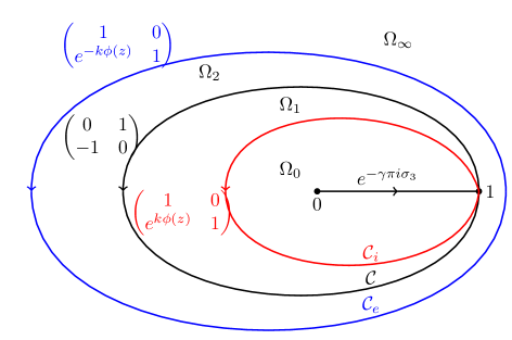
Y~โ€‹(z):=Yโ€‹(z)โ€‹(1โˆ’1z)โˆ’ฮณ2โ€‹ฯƒ3zโˆˆโ„‚โˆ–(ฮฃโˆช[0,1]).formulae-sequenceassign~๐‘Œ๐‘ง๐‘Œ๐‘งsuperscript11๐‘ง๐›พ2subscript๐œŽ3๐‘งโ„‚ฮฃ01\tilde{Y}(z):=Y(z)\left(1-\frac{1}{z}\right)^{-\frac{\gamma}{2}\sigma_{3}}\qquad z\in\mathbb{C}\setminus(\Sigma\cup[0,1])\,. (2.24)

This matrix-valued function Y~โ€‹(z)~๐‘Œ๐‘ง\tilde{Y}(z) satisfies the following Riemann-Hilbert problem:

  1. 1.

    Piecewise analyticity:

    Y~โ€‹(z)โ€‹ย is analytic inย โ€‹โ„‚โˆ–(ฮฃโˆช[0,1])~๐‘Œ๐‘งย is analytic inย โ„‚ฮฃ01\tilde{Y}(z)\text{ is analytic in }\mathbb{C}\setminus(\Sigma\cup[0,1]) (2.25)
  2. 2.

    Jumps on ฮฃฮฃ\Sigma and [0,1]01[0,1]:

    Y~+โ€‹(z)=Y~โˆ’โ€‹(z)โ€‹{(1eโˆ’kโ€‹Vโ€‹(z)01)zโˆˆฮฃ,eโˆ’ฮณโ€‹ฯ€โ€‹iโ€‹ฯƒ3zโˆˆ(0,1),subscript~๐‘Œ๐‘งsubscript~๐‘Œ๐‘งcasesmatrix1superscript๐‘’๐‘˜๐‘‰๐‘ง01๐‘งฮฃmissing-subexpressionmissing-subexpressionsuperscript๐‘’๐›พ๐œ‹๐‘–subscript๐œŽ3๐‘ง01\tilde{Y}_{+}(z)=\tilde{Y}_{-}(z)\left\{\begin{array}[]{cl}\displaystyle\begin{pmatrix}1&e^{-kV(z)}\\ 0&1\end{pmatrix}&\quad z\in\Sigma,\\ &\\ \displaystyle e^{-\gamma\pi i\sigma_{3}}&\quad z\in(0,1),\end{array}\right.

    with Vโ€‹(z)๐‘‰๐‘งV(z) as (2.11).

  3. 3.

    Behaviour at z=โˆž๐‘งz=\infty:

    Y~โ€‹(z)=(I+๐’ชโ€‹(1z))โ€‹zkโ€‹ฯƒ3,zโ†’โˆž.formulae-sequence~๐‘Œ๐‘ง๐ผ๐’ช1๐‘งsuperscript๐‘ง๐‘˜subscript๐œŽ3โ†’๐‘ง\tilde{Y}(z)=\left(I+{\mathcal{O}}\left(\frac{1}{z}\right)\right)z^{k\sigma_{3}}\ ,\quad z\to\infty\ . (2.26)
  4. 4.

    Endpoint behaviour at z=0๐‘ง0z=0 and at z=1๐‘ง1z=1:

    Y~โ€‹(z)โ€‹zโˆ’ฮณ2โ€‹ฯƒ3=๐’ชโ€‹(1)zโ†’0,Y~โ€‹(z)โ€‹(zโˆ’1)ฮณ2โ€‹ฯƒ3=๐’ชโ€‹(1)zโ†’1.formulae-sequence~๐‘Œ๐‘งsuperscript๐‘ง๐›พ2subscript๐œŽ3๐’ช1formulae-sequenceโ†’๐‘ง0formulae-sequence~๐‘Œ๐‘งsuperscript๐‘ง1๐›พ2subscript๐œŽ3๐’ช1โ†’๐‘ง1\tilde{Y}(z)z^{-\frac{\gamma}{2}\sigma_{3}}={\mathcal{O}}\left(1\right)\quad z\to 0\ ,\qquad\tilde{Y}(z)(z-1)^{\frac{\gamma}{2}\sigma_{3}}={\mathcal{O}}\left(1\right)\quad z\to 1\ . (2.27)

The polynomials ฯ€kโ€‹(z)subscript๐œ‹๐‘˜๐‘ง\pi_{k}(z) is recovered from Y~โ€‹(z)~๐‘Œ๐‘ง\tilde{Y}(z) as

ฯ€kโ€‹(z)=Y~11โ€‹(z)โ€‹(1โˆ’1z)ฮณ2.subscript๐œ‹๐‘˜๐‘งsubscript~๐‘Œ11๐‘งsuperscript11๐‘ง๐›พ2\pi_{k}(z)=\tilde{Y}_{11}(z)\left(1-\frac{1}{z}\right)^{\frac{\gamma}{2}}.

3 Asymptotic analysis in the pre-critical case

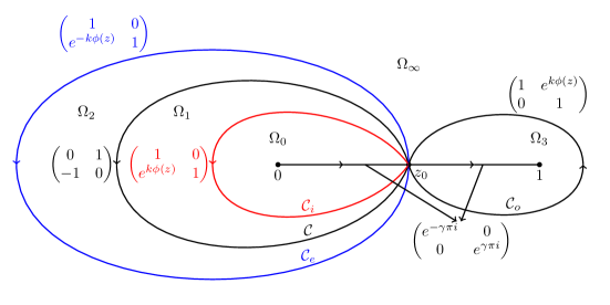
In order to analyse the large k๐‘˜k behaviour of Y~โ€‹(z)~๐‘Œ๐‘ง\tilde{Y}(z) we use the Deiftโ€“Zhou nonlinear steepest descent method [22]. The first step to study the large k๐‘˜k behaviour of the matrix function Y~โ€‹(z)~๐‘Œ๐‘ง\tilde{Y}(z) is to make a transformation Y~โ€‹(z)โ†’Uโ€‹(z)โ†’~๐‘Œ๐‘ง๐‘ˆ๐‘ง\tilde{Y}(z)\to U(z) so that the Riemannโ€“Hilbert problem for Uโ€‹(z)๐‘ˆ๐‘งU(z) is normalised to the identity as |z|โ†’โˆžโ†’๐‘ง|z|\to\infty. For this purpose we introduce a contour ๐’ž๐’ž\mathcal{C} homotopically equivalent to ฮฃฮฃ\Sigma in โ„‚โˆ–[0,1]โ„‚01\mathbb{C}\setminus[0,1] and a function gโ€‹(z)๐‘”๐‘งg(z) analytic off ๐’ž๐’ž\mathcal{C}. Both the contour ๐’ž๐’ž\mathcal{C} and the function gโ€‹(z)๐‘”๐‘งg(z) will be determined later. We assume that the function gโ€‹(z)๐‘”๐‘งg(z) is of the form

gโ€‹(z)=โˆซ๐’žlogโก(zโˆ’s)โ€‹๐‘‘ฮฝโ€‹(s),๐‘”๐‘งsubscript๐’ž๐‘ง๐‘ differential-d๐œˆ๐‘ g(z)=\int_{\mathcal{C}}\log(z-s)d\nu(s), (3.1)

where dโ€‹ฮฝโ€‹(s)๐‘‘๐œˆ๐‘ d\nu(s) is a positive measure with support on ๐’ž๐’ž\mathcal{C} such that

โˆซ๐’ž๐‘‘ฮฝโ€‹(s)=1.subscript๐’ždifferential-d๐œˆ๐‘ 1\int_{\mathcal{C}}d\nu(s)=1.

With this assumption clearly one has

gโ€‹(z)=logโกz+๐’ชโ€‹(zโˆ’1)azย |z|โ†’โˆž,๐‘”๐‘ง๐‘ง๐’ชsuperscript๐‘ง1azย |z|โ†’โˆžg(z)=\log z+{\mathcal{O}}\left(z^{-1}\right)\quad\mbox{az $|z|\to\infty$}, (3.2)

where the logarithm is branched on the positive real axis.

3.1 First transformation Y~โ†’Uโ†’~๐‘Œ๐‘ˆ\tilde{Y}\to U

Since ๐’ž๐’ž\mathcal{C} is homotopically equivalent to ฮฃฮฃ\Sigma in โ„‚โˆ–[0,1]โ„‚01\mathbb{C}\setminus[0,1] we can deform the contour ฮฃฮฃ\Sigma appearing in the Riemannโ€“Hilbert problem for Y~~๐‘Œ\tilde{Y} to ๐’ž๐’ž\mathcal{C}. Define the modified matrix

Uโ€‹(z)=eโˆ’kโ€‹(โ„“/2)โ€‹ฯƒ3โ€‹Y~โ€‹(z)โ€‹eโˆ’kโ€‹gโ€‹(z)โ€‹ฯƒ3โ€‹ekโ€‹(โ„“/2)โ€‹ฯƒ3zโˆˆโ„‚โˆ–(๐’žโˆช[0,1]),formulae-sequence๐‘ˆ๐‘งsuperscript๐‘’๐‘˜โ„“2subscript๐œŽ3~๐‘Œ๐‘งsuperscript๐‘’๐‘˜๐‘”๐‘งsubscript๐œŽ3superscript๐‘’๐‘˜โ„“2subscript๐œŽ3๐‘งโ„‚๐’ž01U(z)=e^{-k(\ell/2)\sigma_{3}}\tilde{Y}(z)e^{-kg(z)\sigma_{3}}e^{k(\ell/2)\sigma_{3}}\qquad z\in\mathbb{C}\setminus(\mathcal{C}\cup[0,1]), (3.3)

where โ„“โ„“\ell is a real number, to be determined below. Then Uโ€‹(z)๐‘ˆ๐‘งU(z) solves the following RHP problem

  1. 1.

    Piecewise analyticity:

    Uโ€‹(z)โ€‹ย is analytic inย โ€‹โ„‚โˆ–(๐’žโˆช[0,1]).๐‘ˆ๐‘งย is analytic inย โ„‚๐’ž01U(z)\text{ is analytic in }\mathbb{C}\setminus(\mathcal{C}\cup[0,1]). (3.4)
  2. 2.

    Jump discontinuity on ๐’ž๐’ž\mathcal{C}:

    U+โ€‹(z)=Uโˆ’โ€‹(z)โ€‹(eโˆ’kโ€‹(g+โˆ’gโˆ’)ekโ€‹(g++gโˆ’โˆ’โ„“โˆ’V)0ekโ€‹(g+โˆ’gโˆ’)),subscript๐‘ˆ๐‘งsubscript๐‘ˆ๐‘งmatrixsuperscript๐‘’๐‘˜subscript๐‘”subscript๐‘”superscript๐‘’๐‘˜subscript๐‘”subscript๐‘”โ„“๐‘‰0superscript๐‘’๐‘˜subscript๐‘”subscript๐‘”U_{+}(z)=U_{-}(z)\begin{pmatrix}e^{-k(g_{+}-g_{-})}&e^{k(g_{+}+g_{-}-\ell-V)}\\ 0&e^{k(g_{+}-g_{-})}\end{pmatrix}\ , (3.5)
  3. 3.

    Jump discontinuity on (0,1)01(0,1):

    U+โ€‹(z)=Uโˆ’โ€‹(z)โ€‹eโˆ’ฮณโ€‹ฯ€โ€‹iโ€‹ฯƒ3,subscript๐‘ˆ๐‘งsubscript๐‘ˆ๐‘งsuperscript๐‘’๐›พ๐œ‹๐‘–subscript๐œŽ3U_{+}(z)=U_{-}(z)e^{-\gamma\pi i\sigma_{3}}\ , (3.6)
  4. 4.

    Endpoint behaviour at z=0๐‘ง0z=0 and z=1๐‘ง1z=1:

    Uโ€‹(z)โ€‹zโˆ’ฮณ2โ€‹ฯƒ3=๐’ชโ€‹(1)zโ†’0,Uโ€‹(z)โ€‹(zโˆ’1)ฮณ2โ€‹ฯƒ3=๐’ชโ€‹(1)zโ†’1.formulae-sequence๐‘ˆ๐‘งsuperscript๐‘ง๐›พ2subscript๐œŽ3๐’ช1formulae-sequenceโ†’๐‘ง0formulae-sequence๐‘ˆ๐‘งsuperscript๐‘ง1๐›พ2subscript๐œŽ3๐’ช1โ†’๐‘ง1U(z)z^{-\frac{\gamma}{2}\sigma_{3}}={\mathcal{O}}\left(1\right)\quad z\to 0\ ,\qquad U(z)(z-1)^{\frac{\gamma}{2}\sigma_{3}}={\mathcal{O}}\left(1\right)\quad z\to 1\ . (3.7)
  5. 5.

    Large z๐‘งz boundary behaviour:

    Uโ€‹(z)=I+๐’ชโ€‹(1z),zโ†’โˆž.formulae-sequence๐‘ˆ๐‘ง๐ผ๐’ช1๐‘งโ†’๐‘งU(z)=I+{\mathcal{O}}\left(\frac{1}{z}\right)\ ,\quad z\to\infty\ . (3.8)

The polynomial ฯ€kโ€‹(z)subscript๐œ‹๐‘˜๐‘ง\pi_{k}(z) is determined from Uโ€‹(z)๐‘ˆ๐‘งU(z) by

ฯ€kโ€‹(z)=U11โ€‹(z)โ€‹ekโ€‹gโ€‹(z)โ€‹(1โˆ’1z)ฮณ2.subscript๐œ‹๐‘˜๐‘งsubscript๐‘ˆ11๐‘งsuperscript๐‘’๐‘˜๐‘”๐‘งsuperscript11๐‘ง๐›พ2\pi_{k}(z)=U_{11}(z)e^{kg(z)}\left(1-\frac{1}{z}\right)^{\frac{\gamma}{2}}. (3.9)

3.1.1 The choice of g๐‘”g-function

In order to determine the function g๐‘”g and the contour ๐’ž๐’ž\mathcal{C} we impose that the jump matrix (3.5) becomes purely oscillatory for large k๐‘˜k. This is accomplished if the following conditions are satisfied:

g+โ€‹(z)+gโˆ’โ€‹(z)โˆ’โ„“โˆ’Vโ€‹(z)=0Reโก(g+โ€‹(z)โˆ’gโˆ’โ€‹(z))=0zโˆˆ๐’ž.subscript๐‘”๐‘งsubscript๐‘”๐‘งโ„“๐‘‰๐‘ง0Resubscript๐‘”๐‘งsubscript๐‘”๐‘ง0๐‘ง๐’ž\begin{split}g_{+}(z)+g_{-}(z)-\ell-V(z)&=0\\ \operatorname{Re}(g_{+}(z)-g_{-}(z))&=0\end{split}\qquad z\in\mathcal{C}. (3.10)

Next we show that we can find a function g๐‘”g and a contour ๐’ž๐’ž\mathcal{C} that satisfy the conditions (3.10). For the purpose we use the following elementary result in the theory of boundary value problems.

Lemma 3.1 ([29], p.ย 78).

Let L๐ฟL be a simple closed contour dividing the complex plane in two regions D+subscript๐ทD_{+} and Dโˆ’subscript๐ทD_{-} where D+=Int(L)subscript๐ทInt๐ฟD_{+}=\operatornamewithlimits{Int}(L) and Dโˆ’=Ext(L)subscript๐ทExt๐ฟD_{-}=\operatornamewithlimits{Ext}(L). Suppose that a function ฯˆโ€‹(ฮถ)๐œ“๐œ\psi(\zeta) defined on L๐ฟL can be represented in the form

ฯˆโ€‹(ฮถ)=ฯˆ+โ€‹(ฮถ)+ฯˆโˆ’โ€‹(ฮถ),ฮถโˆˆLformulae-sequence๐œ“๐œsubscript๐œ“๐œsubscript๐œ“๐œ๐œ๐ฟ\psi(\zeta)=\psi_{+}(\zeta)+\psi_{-}(\zeta),\quad\zeta\in L

where ฯˆ+โ€‹(ฮถ)subscript๐œ“๐œ\psi_{+}(\zeta) is the boundary value of a function ฯˆ+โ€‹(z)subscript๐œ“๐‘ง\psi_{+}(z) analytic for zโˆˆD+๐‘งsubscript๐ทz\in D_{+} and ฯˆโˆ’โ€‹(ฮถ)subscript๐œ“๐œ\psi_{-}(\zeta) is the boundary value of a function ฯˆโˆ’โ€‹(z)subscript๐œ“๐‘ง\psi_{-}(z) analytic for zโˆˆDโˆ’๐‘งsubscript๐ทz\in D_{-} and such that ฯˆโˆ’โ€‹(โˆž)=0subscript๐œ“0\psi_{-}(\infty)=0. Then the Cauchy integral

ฮฆโ€‹(z)=12โ€‹ฯ€โ€‹iโ€‹โˆซLฯˆโ€‹(ฮถ)ฮถโˆ’zโ€‹๐‘‘ฮถ,ฮฆ๐‘ง12๐œ‹๐‘–subscript๐ฟ๐œ“๐œ๐œ๐‘งdifferential-d๐œ\Phi(z)=\dfrac{1}{2\pi i}\int_{L}\dfrac{\psi(\zeta)}{\zeta-z}d\zeta,

can be represented in the form

ฮฆ+โ€‹(z)=ฯˆ+โ€‹(z),ย forย zโˆˆD+,ฮฆโˆ’โ€‹(z)=โˆ’ฯˆโˆ’โ€‹(z),forย zโˆˆDโˆ’.\begin{split}&\Phi_{+}(z)=\psi_{+}(z),\quad\text{ for $z\in D_{+}$},\\ &\Phi_{-}(z)=-\psi_{-}(z),\quad\text{for $z\in D_{-}$}.\end{split} (3.11)

The boundary values of the function ฮฆฮฆ\Phi on the two sides of the contour L๐ฟL then satisfy

ฮฆ+โ€‹(ฮถ)+ฮฆโˆ’โ€‹(ฮถ)=ฯˆ+โ€‹(ฮถ)โˆ’ฯˆโˆ’โ€‹(ฮถ)ฮฆ+โ€‹(ฮถ)โˆ’ฮฆโˆ’โ€‹(ฮถ)=ฯˆ+โ€‹(ฮถ)+ฯˆโˆ’โ€‹(ฮถ)ฮถโˆˆL.subscriptฮฆ๐œsubscriptฮฆ๐œsubscript๐œ“๐œsubscript๐œ“๐œsubscriptฮฆ๐œsubscriptฮฆ๐œsubscript๐œ“๐œsubscript๐œ“๐œ๐œ๐ฟ\begin{split}&\Phi_{+}(\zeta)+\Phi_{-}(\zeta)=\psi_{+}(\zeta)-\psi_{-}(\zeta)\\ &\Phi_{+}(\zeta)-\Phi_{-}(\zeta)=\psi_{+}(\zeta)+\psi_{-}(\zeta)\end{split}\qquad\zeta\in L. (3.12)

Now we apply Lemmaย 3.1 to the function gโ€ฒโ€‹(z)superscript๐‘”โ€ฒ๐‘งg^{\prime}(z) that satisfies the differentiated boundary condition

g+โ€ฒโ€‹(ฮถ)+gโˆ’โ€ฒโ€‹(ฮถ)=Vโ€ฒโ€‹(ฮถ)=1z0+1ฮถ,ฮถโˆˆ๐’ž.formulae-sequencesuperscriptsubscript๐‘”โ€ฒ๐œsubscriptsuperscript๐‘”โ€ฒ๐œsuperscript๐‘‰โ€ฒ๐œ1subscript๐‘ง01๐œ๐œ๐’žg_{+}^{\prime}(\zeta)+g^{\prime}_{-}(\zeta)=V^{\prime}(\zeta)=\dfrac{1}{z_{0}}+\dfrac{1}{\zeta},\quad\zeta\in\mathcal{C}.

The functions ฯˆยฑโ€‹(z)subscript๐œ“plus-or-minus๐‘ง\psi_{\pm}(z) of Lemma 3.1 are ฯˆ+โ€‹(z)=1z0subscript๐œ“๐‘ง1subscript๐‘ง0\psi_{+}(z)=\dfrac{1}{z_{0}} and ฯˆโˆ’โ€‹(z)=โˆ’1zsubscript๐œ“๐‘ง1๐‘ง\psi_{-}(z)=-\dfrac{1}{z} and therefore the function gโ€ฒโ€‹(z)superscript๐‘”โ€ฒ๐‘งg^{\prime}(z) takes the form

gโ€ฒโ€‹(z)=12โ€‹ฯ€โ€‹iโ€‹โˆซ๐’ž1ฯ„โˆ’1z0zโˆ’ฯ„โ€‹๐‘‘ฯ„={1z0zโˆˆInt(๐’ž)1zzโˆˆExt(๐’ž),superscript๐‘”โ€ฒ๐‘ง12๐œ‹๐‘–subscript๐’ž1๐œ1subscript๐‘ง0๐‘ง๐œdifferential-d๐œcases1subscript๐‘ง0๐‘งInt๐’žmissing-subexpressionmissing-subexpression1๐‘ง๐‘งExt๐’žg^{\prime}(z)=\dfrac{1}{2\pi i}\int_{\mathcal{C}}\dfrac{\frac{1}{\tau}-\frac{1}{z_{0}}}{z-\tau}d\tau=\left\{\begin{array}[]{ll}\displaystyle\frac{1}{z_{0}}&z\in\operatornamewithlimits{Int}(\mathcal{C})\\ &\\ \displaystyle\frac{1}{z}&z\in\operatornamewithlimits{Ext}(\mathcal{C})\,,\end{array}\right. (3.13)

so that the measure dโ€‹ฮฝ๐‘‘๐œˆd\nu in (3.1) is given by

dโ€‹ฮฝโ€‹(z)=12โ€‹ฯ€โ€‹iโ€‹(1zโˆ’1z0)โ€‹dโ€‹z,zโˆˆ๐’ž.formulae-sequence๐‘‘๐œˆ๐‘ง12๐œ‹๐‘–1๐‘ง1subscript๐‘ง0๐‘‘๐‘ง๐‘ง๐’žd\nu(z)=\dfrac{1}{2\pi i}\left(\dfrac{1}{z}-\dfrac{1}{z_{0}}\right)dz,\quad z\in\mathcal{C}. (3.14)

Integrating the relation (3.13) and using (3.2) one has

gโ€‹(z)={zz0+โ„“zโˆˆInt(๐’ž)logโกzzโˆˆExt(๐’ž),๐‘”๐‘งcases๐‘งsubscript๐‘ง0โ„“๐‘งInt๐’žmissing-subexpressionmissing-subexpression๐‘ง๐‘งExt๐’žg(z)=\left\{\begin{array}[]{ll}\displaystyle\frac{z}{z_{0}}+\ell&z\in\operatornamewithlimits{Int}(\mathcal{C})\\ &\\ \displaystyle\log z&z\in\operatornamewithlimits{Ext}(\mathcal{C})\end{array},\right. (3.15)

where โ„“โ„“\ell is an integration constant and logโกz๐‘ง\log z is analytic in โ„‚\โ„+\โ„‚superscriptโ„\mathbb{C}\backslash\mathbb{R}^{+}. Performing the integral in (3.1) for a specific value of zโˆˆ๐’ž๐‘ง๐’žz\in\mathcal{C}, say z=0๐‘ง0z=0 and deforming ๐’ž๐’ž\mathcal{C} to a circle of radius r๐‘Ÿr one can determine the value of โ„“โ„“\ell:

โ„“=logโกrโˆ’rz0,r>0.formulae-sequenceโ„“๐‘Ÿ๐‘Ÿsubscript๐‘ง0๐‘Ÿ0\ell=\log r-\dfrac{r}{z_{0}},\quad r>0. (3.16)

The total integral of dโ€‹ฮฝ๐‘‘๐œˆd\nu in (3.14) is normalized to one on any closed contour containing the point z=0๐‘ง0z=0. However we have to define the contour ๐’ž๐’ž\mathcal{C} so that dโ€‹ฮฝโ€‹(z)๐‘‘๐œˆ๐‘งd\nu(z) is a real and positive measure along ๐’ž๐’ž\mathcal{C}. To this end we introduce the function

ฯ•rโ€‹(z)={โˆ’2โ€‹gโ€‹(z)+Vโ€‹(z)+logโกrโˆ’rz0=logโกzโˆ’zz0โˆ’logโกr+rz0zโˆˆInt(๐’ž)\[0,r]2โ€‹gโ€‹(z)โˆ’Vโ€‹(z)โˆ’logโกr+rz0=logโกzโˆ’zz0โˆ’logโกr+rz0zโˆˆExt(๐’ž)\(r,โˆž).subscriptitalic-ฯ•๐‘Ÿ๐‘งcases2๐‘”๐‘ง๐‘‰๐‘ง๐‘Ÿ๐‘Ÿsubscript๐‘ง0๐‘ง๐‘งsubscript๐‘ง0๐‘Ÿ๐‘Ÿsubscript๐‘ง0๐‘ง\Int๐’ž0๐‘Ÿmissing-subexpressionmissing-subexpression2๐‘”๐‘ง๐‘‰๐‘ง๐‘Ÿ๐‘Ÿsubscript๐‘ง0๐‘ง๐‘งsubscript๐‘ง0๐‘Ÿ๐‘Ÿsubscript๐‘ง0๐‘ง\Ext๐’ž๐‘Ÿ\phi_{r}(z)=\left\{\begin{array}[]{ll}-2g(z)+V(z)+\log r-\dfrac{r}{z_{0}}=\log z-\dfrac{z}{z_{0}}-\log r+\dfrac{r}{z_{0}}&z\in\operatornamewithlimits{Int}(\mathcal{C})\backslash[0,r]\\ &\\ 2g(z)-V(z)-\log r+\dfrac{r}{z_{0}}=\log z-\dfrac{z}{z_{0}}-\log r+\dfrac{r}{z_{0}}&z\in\operatornamewithlimits{Ext}(\mathcal{C})\backslash(r,\infty)\ .\end{array}\right. (3.17)

Observe that ฯ•rโ€‹(z)subscriptitalic-ฯ•๐‘Ÿ๐‘ง\phi_{r}(z) is analytic across ๐’ž๐’ž\mathcal{C}, namely ฯ•r+โ€‹(z)=ฯ•rโˆ’โ€‹(z)subscriptitalic-ฯ•limit-from๐‘Ÿ๐‘งsubscriptitalic-ฯ•limit-from๐‘Ÿ๐‘ง\phi_{r+}(z)=\phi_{r-}(z), zโˆˆ๐’ž๐‘ง๐’žz\in\mathcal{C} and that

ฯ•rโ€‹(z)=ฯ•r+โ€‹(z)+ฯ•rโˆ’โ€‹(z)2=โˆ’g+โ€‹(z)+gโˆ’โ€‹(z),zโˆˆ๐’ž.formulae-sequencesubscriptitalic-ฯ•๐‘Ÿ๐‘งsubscriptitalic-ฯ•limit-from๐‘Ÿ๐‘งsubscriptitalic-ฯ•limit-from๐‘Ÿ๐‘ง2subscript๐‘”๐‘งsubscript๐‘”๐‘ง๐‘ง๐’ž\phi_{r}(z)=\dfrac{\phi_{r+}(z)+\phi_{r-}(z)}{2}=-g_{+}(z)+g_{-}(z),\quad z\in\mathcal{C}. (3.18)

The next identity follows in a trivial way

dโ€‹ฮฝโ€‹(z)=12โ€‹ฯ€โ€‹iโ€‹dโ€‹ฯ•rโ€‹(z).๐‘‘๐œˆ๐‘ง12๐œ‹๐‘–๐‘‘subscriptitalic-ฯ•๐‘Ÿ๐‘งd\nu(z)=\dfrac{1}{2\pi i}d\phi_{r}(z).

Imposing the relation (3.10) on (3.18) one has

Reโก(ฯ•rโ€‹(z))=logโก|z|โˆ’Reโก(z)z0โˆ’logโกr+rz0=0.Resubscriptitalic-ฯ•๐‘Ÿ๐‘ง๐‘งRe๐‘งsubscript๐‘ง0๐‘Ÿ๐‘Ÿsubscript๐‘ง00\operatorname{Re}(\phi_{r}(z))=\log|z|-\frac{\operatorname{Re}(z)}{z_{0}}-\log r+\dfrac{r}{z_{0}}=0. (3.19)

This equation defines a family of contours which are closed for |z|โ‰คr๐‘ง๐‘Ÿ|z|\leq r (easy to verify). Since the function โˆ’logโกr+rz0๐‘Ÿ๐‘Ÿsubscript๐‘ง0-\log r+\dfrac{r}{z_{0}} for r>0๐‘Ÿ0r>0 has a single minimum at r=z0๐‘Ÿsubscript๐‘ง0r=z_{0} and diverge to +โˆž+\infty for rโ†’0โ†’๐‘Ÿ0r\to 0 and rโ†’โˆžโ†’๐‘Ÿr\to\infty, it is sufficient to consider only the values 0<rโ‰คz00๐‘Ÿsubscript๐‘ง00<r\leq z_{0}.

We define the contour ๐’žrsubscript๐’ž๐‘Ÿ\mathcal{C}_{r} associated to r๐‘Ÿr as (see Figureย 3.1)

๐’žr={zโˆˆโ„‚:Reโก(ฯ•rโ€‹(z))=0,|z|โ‰คz0},0<rโ‰คz0.formulae-sequencesubscript๐’ž๐‘Ÿconditional-set๐‘งโ„‚formulae-sequenceResubscriptitalic-ฯ•๐‘Ÿ๐‘ง0๐‘งsubscript๐‘ง00๐‘Ÿsubscript๐‘ง0\mathcal{C}_{r}=\{z\in\mathbb{C}\ \colon\ \operatorname{Re}(\phi_{r}(z))=0,\;\;|z|\leq z_{0}\},\quad 0<r\leq z_{0}. (3.20)
Refer to caption
Figure 3.1: The family of contours ๐’žrsubscript๐’ž๐‘Ÿ\mathcal{C}_{r} for three values of r๐‘Ÿr: r=z0๐‘Ÿsubscript๐‘ง0r=z_{0}, r=1๐‘Ÿ1r=1 and r<1๐‘Ÿ1r<1. For r=z0๐‘Ÿsubscript๐‘ง0r=z_{0}, the region |z|>z0๐‘งsubscript๐‘ง0|z|>z_{0} is plotted as well.

Since โˆ‚xReโกฯ•r|y=0=|x|x2โˆ’1z0>0evaluated-atsubscript๐‘ฅResubscriptitalic-ฯ•๐‘Ÿ๐‘ฆ0๐‘ฅsuperscript๐‘ฅ21subscript๐‘ง00\partial_{x}\operatorname{Re}\phi_{r}|_{y=0}=\dfrac{|x|}{x^{2}}-\dfrac{1}{z_{0}}>0, for |x|<z0๐‘ฅsubscript๐‘ง0|x|<z_{0}, Reโกฯ•rโ€‹(z)Resubscriptitalic-ฯ•๐‘Ÿ๐‘ง\operatorname{Re}\phi_{r}(z) is negative inside ๐’žrsubscript๐’ž๐‘Ÿ\mathcal{C}_{r}. Note that the point z=0๐‘ง0z=0 lies inside ๐’žrsubscript๐’ž๐‘Ÿ\mathcal{C}_{r} since Reโกฯ•โ€‹(z)โ†’โˆ’โˆžโ†’Reitalic-ฯ•๐‘ง\operatorname{Re}\,\phi(z)\to-\infty for |z|โ†’0โ†’๐‘ง0|z|\to 0. Furthermore ๐’žrsubscript๐’ž๐‘Ÿ\mathcal{C}_{r} intersects the real line in the points z=r๐‘ง๐‘Ÿz=r and zโˆˆ(โˆ’r,0)๐‘ง๐‘Ÿ0z\in(-r,0). Indeed Reโกฯ•โ€‹(โˆ’r)>0Reitalic-ฯ•๐‘Ÿ0\operatorname{Re}\,\phi(-r)>0 which shows that the point z=โˆ’r๐‘ง๐‘Ÿz=-r lies outside ๐’žrsubscript๐’ž๐‘Ÿ\mathcal{C}_{r}.

Lemma 3.2.

The a-priori complex measure ฮฝ๐œˆ\nu in (3.14) is a probability measure on the contour ๐’žrsubscript๐’ž๐‘Ÿ\mathcal{C}_{r} defined in (3.20) for 0<rโ‰คz00๐‘Ÿsubscript๐‘ง00<r\leq z_{0}.

Proof.ย By the Residue Theorem the measure dโ€‹ฮฝ๐‘‘๐œˆd\nu has total mass 111 on any contour ๐’žrsubscript๐’ž๐‘Ÿ\mathcal{C}_{r}. Since Reโกฯ•r=0Resubscriptitalic-ฯ•๐‘Ÿ0\operatorname{Re}\phi_{r}=0 on the contour ๐’žrsubscript๐’ž๐‘Ÿ\mathcal{C}_{r} it follows that the measure dโ€‹ฮฝ=12โ€‹ฯ€โ€‹iโ€‹dโ€‹ฯ•r๐‘‘๐œˆ12๐œ‹๐‘–๐‘‘subscriptitalic-ฯ•๐‘Ÿd\nu=\dfrac{1}{2\pi i}d\phi_{r} is real on the contour ๐’žrsubscript๐’ž๐‘Ÿ\mathcal{C}_{r}. In order to show that the measure is positive on the contour ๐’žrsubscript๐’ž๐‘Ÿ\mathcal{C}_{r} we introduce the variable

ฯˆr=eฯ•r,subscript๐œ“๐‘Ÿsuperscript๐‘’subscriptitalic-ฯ•๐‘Ÿ\psi_{r}=e^{\phi_{r}},

On the contour ๐’žrsubscript๐’ž๐‘Ÿ\mathcal{C}_{r} we have that |ฯˆr|=1subscript๐œ“๐‘Ÿ1|\psi_{r}|=1, so that in the ฯˆrsubscript๐œ“๐‘Ÿ\psi_{r}โ€“plane the contour ๐’žrsubscript๐’ž๐‘Ÿ\mathcal{C}_{r} is mapped to a circle of radius one and the map ฯˆr=eฯ•rsubscript๐œ“๐‘Ÿsuperscript๐‘’subscriptitalic-ฯ•๐‘Ÿ\psi_{r}=e^{\phi_{r}} is a univalent conformal map from the interior of ๐’žrsubscript๐’ž๐‘Ÿ\mathcal{C}_{r} to the interior of a circle [52]. We have

dโ€‹ฮฝ=12โ€‹ฯ€โ€‹iโ€‹dโ€‹ฯˆrฯˆr,๐‘‘๐œˆ12๐œ‹๐‘–๐‘‘subscript๐œ“๐‘Ÿsubscript๐œ“๐‘Ÿd\nu=\dfrac{1}{2\pi i}\dfrac{d\psi_{r}}{\psi_{r}},

which shows that the measure dโ€‹ฮฝ๐‘‘๐œˆd\nu in the variable ฯˆrsubscript๐œ“๐‘Ÿ\psi_{r} is a uniform measure on the circle and therefore dโ€‹ฮฝ๐‘‘๐œˆd\nu is a positive measure on each contour ๐’žrsubscript๐’ž๐‘Ÿ\mathcal{C}_{r}. Q.E.D.
We are now ready to prove Lemmaย 1.3 and Lemmaย 1.6 announced in the Introduction.

Proof of Lemmaย 1.3. By using the Residue Theorem, it is straightforward to check that dโ€‹ฮฝ^๐‘‘^๐œˆd\hat{\nu} is a probability measure on any contour ๐’ž^rsubscript^๐’ž๐‘Ÿ\hat{\mathcal{C}}_{r} defined in (1.22). In the post-critical case such curve ๐’ž^rsubscript^๐’ž๐‘Ÿ\hat{\mathcal{C}}_{r} has s๐‘ s connected components ๐’ž^rjsubscriptsuperscript^๐’ž๐‘—๐‘Ÿ\hat{\mathcal{C}}^{j}_{r}, j=0,โ€ฆ,sโˆ’1๐‘—0โ€ฆ๐‘ 1j=0,\dots,s-1, each encircling exactly one root of the equation ฮปs=tsuperscript๐œ†๐‘ ๐‘ก\lambda^{s}=t. In the pre-critical case we denote with the same symbol ๐’ž^rjsubscriptsuperscript^๐’ž๐‘—๐‘Ÿ\hat{\mathcal{C}}^{j}_{r} the connected components of ๐’ž^rโˆ–{0}subscript^๐’ž๐‘Ÿ0\hat{\mathcal{C}}_{r}\setminus\{0\} together with {0}0\{0\}.

With the appropriate choice of the branch of the sthsuperscript๐‘ ths^{\text{th}} root, any ๐’ž^rjsuperscriptsubscript^๐’ž๐‘Ÿ๐‘—\hat{\mathcal{C}}_{r}^{j} can be parametrised by the map ฮปโ€‹(z):=(โˆ’tโ€‹(zโˆ’1))1sassign๐œ†๐‘งsuperscript๐‘ก๐‘ง11๐‘ \lambda(z):=(-t(z-1))^{\frac{1}{s}}, which respects the orientations of ๐’ž๐’ž\mathcal{C} and ๐’ž^rjsubscriptsuperscript^๐’ž๐‘—๐‘Ÿ\hat{\mathcal{C}}^{j}_{r} . Since ฯ•โ€‹(z)=ฯ•^โ€‹(ฮปโ€‹(z))italic-ฯ•๐‘ง^italic-ฯ•๐œ†๐‘ง\phi(z)=\hat{\phi}(\lambda(z)), equation (1.23) implies

dโ€‹ฮฝ^โ€‹(ฮปโ€‹(z))=1sโ€‹dโ€‹ฮฝโ€‹(z).๐‘‘^๐œˆ๐œ†๐‘ง1๐‘ ๐‘‘๐œˆ๐‘งd\hat{\nu}(\lambda(z))=\frac{1}{s}d\nu(z)\ .

This relation, together with Lemmaย 3.2, where we proved that dโ€‹ฮฝโ€‹(z)๐‘‘๐œˆ๐‘งd\nu(z) is real and positive on ๐’žrsubscript๐’ž๐‘Ÿ\mathcal{C}_{r}, implies that also dโ€‹ฮฝ^๐‘‘^๐œˆd\hat{\nu} is real and positive on any ๐’ž^rjsubscriptsuperscript^๐’ž๐‘—๐‘Ÿ\hat{\mathcal{C}}^{j}_{r} and hence on the whole ๐’ž^rsubscript^๐’ž๐‘Ÿ\hat{\mathcal{C}}_{r}. Q.E.D.

Proof of Lemmaย 1.6. By using the Residue Theorem we first calculate the r.h.s. of (1.28) obtaining

โˆซ๐’ž^dโ€‹ฮฝ^โ€‹(ฮท)ฮปโˆ’ฮท=12โ€‹ฯ€โ€‹iโ€‹โˆซ๐’ž^ฮทsโˆ’1ฮปโˆ’ฮทโ€‹(1ฮทsโˆ’t+1z0โ€‹t)โ€‹๐‘‘ฮท=ฮปsโˆ’1ฮปsโˆ’t.subscript^๐’ž๐‘‘^๐œˆ๐œ‚๐œ†๐œ‚12๐œ‹๐‘–subscript^๐’žsuperscript๐œ‚๐‘ 1๐œ†๐œ‚1superscript๐œ‚๐‘ ๐‘ก1subscript๐‘ง0๐‘กdifferential-d๐œ‚superscript๐œ†๐‘ 1superscript๐œ†๐‘ ๐‘ก\int_{\hat{\mathcal{C}}}\dfrac{d\hat{\nu}(\eta)}{\lambda-\eta}=\dfrac{1}{2\pi i}\int_{\hat{\mathcal{C}}}\dfrac{\eta^{s-1}}{\lambda-\eta}\left(\dfrac{1}{\eta^{s}-t}+\dfrac{1}{z_{0}t}\right)d\eta=\dfrac{\lambda^{s-1}}{\lambda^{s}-t}. (3.21)

Therefore (1.28) is equivalent to

sโ€‹ฮปsโˆ’1โ€‹(ฮปยฏsโˆ’t)T=ฮปsโˆ’1ฮปsโˆ’t,or(ฮปยฏsโˆ’t)โ€‹(ฮปsโˆ’t)=Ts=tc2,formulae-sequence๐‘ superscript๐œ†๐‘ 1superscriptยฏ๐œ†๐‘ ๐‘ก๐‘‡superscript๐œ†๐‘ 1superscript๐œ†๐‘ ๐‘กorsuperscriptยฏ๐œ†๐‘ ๐‘กsuperscript๐œ†๐‘ ๐‘ก๐‘‡๐‘ superscriptsubscript๐‘ก๐‘2\dfrac{s\lambda^{s-1}(\bar{\lambda}^{s}-t)}{T}=\dfrac{\lambda^{s-1}}{\lambda^{s}-t},\quad\mbox{or}\quad(\bar{\lambda}^{s}-t)(\lambda^{s}-t)=\dfrac{T}{s}=t_{c}^{2},

which is equivalent to the equation for the boundary of D๐ทD defined in (1.12). Next we show that the l.h.s. of (1.29) is equal to its r.h.s. By using Stokesโ€™ Theorem, the relation (1.14) and the Residue Theorem one obtains

โˆซDdโ€‹ฮผโˆ—โ€‹(ฮท)ฮปโˆ’ฮท=12โ€‹ฯ€โ€‹iโ€‹tc2โ€‹โˆซโˆ‚Dฮทsโˆ’1โ€‹ฮทยฏsโ€‹dโ€‹ฮทฮปโˆ’ฮท=12โ€‹ฯ€โ€‹iโ€‹tc2โ€‹โˆซโˆ‚Dฮทsโˆ’1โ€‹Sโ€‹(ฮท)โ€‹dโ€‹ฮทฮปโˆ’ฮท=ฮปsโˆ’1ฮปsโˆ’tsubscript๐ท๐‘‘superscript๐œ‡๐œ‚๐œ†๐œ‚12๐œ‹๐‘–superscriptsubscript๐‘ก๐‘2subscript๐ทsuperscript๐œ‚๐‘ 1superscriptยฏ๐œ‚๐‘ ๐‘‘๐œ‚๐œ†๐œ‚12๐œ‹๐‘–superscriptsubscript๐‘ก๐‘2subscript๐ทsuperscript๐œ‚๐‘ 1๐‘†๐œ‚๐‘‘๐œ‚๐œ†๐œ‚superscript๐œ†๐‘ 1superscript๐œ†๐‘ ๐‘ก\displaystyle\int_{D}\dfrac{d\mu^{*}(\eta)}{\lambda-\eta}=\dfrac{1}{2\pi it_{c}^{2}}\int_{\partial D}\dfrac{\eta^{s-1}\bar{\eta}^{s}d\eta}{\lambda-\eta}=\dfrac{1}{2\pi it_{c}^{2}}\int_{\partial D}\dfrac{\eta^{s-1}S(\eta)d\eta}{\lambda-\eta}=\dfrac{\lambda^{s-1}}{\lambda^{s}-t} (3.22)

which coincides with (3.21). Q.E.D.

3.1.2 Choice of the contour
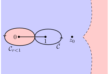
Refer to caption
Figure 3.2: The contour ๐’žr<1โˆช๐’ž~subscript๐’ž๐‘Ÿ1~๐’ž\mathcal{C}_{r<1}\cup\tilde{\mathcal{C}} that is homotopic to ฮฃฮฃ\Sigma. The region where Reโกฯ•โ€‹(z)<0Reitalic-ฯ•๐‘ง0\operatorname{Re}\phi(z)<0 is coloured in red.

We now argue that the relevant contour on which the zeros of the orthogonal polynomials ฯ€kโ€‹(z)subscript๐œ‹๐‘˜๐‘ง\pi_{k}(z) accumulate in the pre-critical case is given by the level r=1๐‘Ÿ1r=1. The family of contours 0<r<10๐‘Ÿ10<r<1 can be immediately ignored because in this case ฮฃฮฃ\Sigma has to be deformed to two contours ฮฃโ‰ƒ๐’žr<1โˆช๐’ž~similar-to-or-equalsฮฃsubscript๐’ž๐‘Ÿ1~๐’ž\Sigma\simeq\mathcal{C}_{r<1}\cup\tilde{\mathcal{C}} as shown in Figureย 3.2. On the contour ๐’ž~~๐’ž\tilde{\mathcal{C}} we have Reโก(ฯ•)>0Reitalic-ฯ•0\operatorname{Re}(\phi)>0 and it is not possible to perform any contour deformation to get exponentially small terms in the jump matrix (3.5) as kโ†’โˆžโ†’๐‘˜k\to\infty.

For 1<rโ‰คz01๐‘Ÿsubscript๐‘ง01<r\leq z_{0} the original contour ฮฃฮฃ\Sigma can be deformed homotopically to the contours ๐’žrsubscript๐’ž๐‘Ÿ\mathcal{C}_{r}. In this case the asymptotic expansion of the matrix entry Y11โ€‹(z)=ฯ€kโ€‹(z)subscript๐‘Œ11๐‘งsubscript๐œ‹๐‘˜๐‘งY_{11}(z)=\pi_{k}(z) as kโ†’โˆžโ†’๐‘˜k\to\infty, does not give any sub-leading contribution. For this reason we discard this case and we omit the corresponding asymptotic analysis. The only possible case remains r=1๐‘Ÿ1r=1. In this case the analysis as kโ†’โˆžโ†’๐‘˜k\to\infty to the matrix entry Y11โ€‹(z)=ฯ€kโ€‹(z)subscript๐‘Œ11๐‘งsubscript๐œ‹๐‘˜๐‘งY_{11}(z)=\pi_{k}(z) which will performed in subsectionsย 3.2 to 3.5, gives leading and sub-leading terms. The comparison of these two terms enable us to locate the zeros of the polynomial ฯ€kโ€‹(z)subscript๐œ‹๐‘˜๐‘ง\pi_{k}(z) on a contour that lies within a distance ๐’ชโ€‹(logโกk/k)๐’ช๐‘˜๐‘˜{\mathcal{O}}\left(\log k/k\right) from the contour ๐’žr=1subscript๐’ž๐‘Ÿ1\mathcal{C}_{r=1}.

So for the reasons explained above, we are going to perform the asymptotic analysis of the RH-problem (3.5)-(3.8) by deforming the contour ฮฃฮฃ\Sigma to the contour ๐’žr=1subscript๐’ž๐‘Ÿ1\mathcal{C}_{r=1}. For simplicity we denote this contour by ๐’ž๐’ž\mathcal{C}:

๐’ž={zโˆˆโ„‚:logโก|z|โˆ’Reโก(z)z0+1z0=0,|z|โ‰ค1}๐’žconditional-set๐‘งโ„‚formulae-sequence๐‘งRe๐‘งsubscript๐‘ง01subscript๐‘ง00๐‘ง1\mathcal{C}=\left\{z\in\mathbb{C}\ \colon\ \log|z|-\frac{\operatorname{Re}(z)}{z_{0}}+\dfrac{1}{z_{0}}=0,\;\;|z|\leq 1\right\} (3.23)
Refer to caption
Figure 3.3: The jump matrices for Uโ€‹(z)๐‘ˆ๐‘งU(z)

Also, for simplicity, the function ฯ•r=1subscriptitalic-ฯ•๐‘Ÿ1\phi_{r=1} will be referred to as ฯ•italic-ฯ•\phi below:

ฯ•โ€‹(z)=logโกzโˆ’zz0+1z0,italic-ฯ•๐‘ง๐‘ง๐‘งsubscript๐‘ง01subscript๐‘ง0\phi(z)=\log z-\dfrac{z}{z_{0}}+\dfrac{1}{z_{0}}, (3.24)

where logโกz๐‘ง\log z is analytic in โ„‚\(โˆ’โˆž,0]\โ„‚0\mathbb{C}\backslash(-\infty,0]. With this choice of contour, the jump matrices of the RH problem (3.5)-(3.8) for the matrix Uโ€‹(z)๐‘ˆ๐‘งU(z) are summarized in Figure 3.3.

3.2 The second transformation Uโ†ฆTmaps-to๐‘ˆ๐‘‡U\mapsto T

Consider two extra loops ๐’žisubscript๐’ž๐‘–\mathcal{C}_{i} and ๐’žesubscript๐’ž๐‘’\mathcal{C}_{e} as shown in Figure 3.4. These define new domains ฮฉ0subscriptฮฉ0\Omega_{0}, ฮฉ1subscriptฮฉ1\Omega_{1}, ฮฉ2subscriptฮฉ2\Omega_{2} and ฮฉโˆžsubscriptฮฉ\Omega_{\infty}. Define the new matrix-valued function

Tโ€‹(z)={Uโ€‹(z)zโˆˆฮฉโˆžโˆชฮฉ0Uโ€‹(z)โ€‹(10โˆ’ekโ€‹ฯ•โ€‹(z)1)zโˆˆฮฉ1Uโ€‹(z)โ€‹(10eโˆ’kโ€‹ฯ•โ€‹(z)1)zโˆˆฮฉ2.๐‘‡๐‘งcases๐‘ˆ๐‘ง๐‘งsubscriptฮฉsubscriptฮฉ0๐‘ˆ๐‘งmatrix10superscript๐‘’๐‘˜italic-ฯ•๐‘ง1๐‘งsubscriptฮฉ1๐‘ˆ๐‘งmatrix10superscript๐‘’๐‘˜italic-ฯ•๐‘ง1๐‘งsubscriptฮฉ2T(z)=\left\{\begin{array}[]{ll}U(z)&z\in\Omega_{\infty}\cup\Omega_{0}\\ U(z)\begin{pmatrix}1&0\\ -e^{k\phi(z)}&1\end{pmatrix}&z\in\Omega_{1}\\ U(z)\begin{pmatrix}1&0\\ e^{-k\phi(z)}&1\end{pmatrix}&z\in\Omega_{2}\ .\end{array}\right. (3.25)

Then Tโ€‹(z)๐‘‡๐‘งT(z) satisfies the following Riemannโ€“Hilbert problem:

  1. 1.

    Piecewise analyticity:

    Tโ€‹(z)โ€‹ย is analytic inย โ€‹โ„‚โˆ–(๐’žeโˆช๐’žโˆช๐’žiโˆช[0,1])๐‘‡๐‘งย is analytic inย โ„‚subscript๐’ž๐‘’๐’žsubscript๐’ž๐‘–01T(z)\text{ is analytic in }\mathbb{C}\setminus\left(\mathcal{C}_{e}\cup\mathcal{C}\cup\mathcal{C}_{i}\cup[0,1]\right) (3.26)
  1. 2.

    Jump discontinuities on ฮฃT=๐’žeโˆช๐’žโˆช๐’žiโˆช[0,1]subscriptฮฃ๐‘‡subscript๐’ž๐‘’๐’žsubscript๐’ž๐‘–01\Sigma_{T}=\mathcal{C}_{e}\cup\mathcal{C}\cup\mathcal{C}_{i}\cup[0,1]:

    T+โ€‹(z)=Tโˆ’โ€‹(z)โ€‹vTโ€‹(z),zโˆˆฮฃT,formulae-sequencesubscript๐‘‡๐‘งsubscript๐‘‡๐‘งsubscript๐‘ฃ๐‘‡๐‘ง๐‘งsubscriptฮฃ๐‘‡T_{+}(z)=T_{-}(z)v_{T}(z),\quad z\in\Sigma_{T}, (3.27)

    where

    vTโ€‹(z)={(01โˆ’10)zโˆˆ๐’ž(10eโˆ’kโ€‹ฯ•โ€‹(z)1)zโˆˆ๐’že(10ekโ€‹ฯ•โ€‹(z)1)zโˆˆ๐’žieโˆ’ฮณโ€‹ฯ€โ€‹iโ€‹ฯƒ3zโˆˆ(0,1).subscript๐‘ฃ๐‘‡๐‘งcasesmatrix0110๐‘ง๐’žmatrix10superscript๐‘’๐‘˜italic-ฯ•๐‘ง1๐‘งsubscript๐’ž๐‘’matrix10superscript๐‘’๐‘˜italic-ฯ•๐‘ง1๐‘งsubscript๐’ž๐‘–superscript๐‘’๐›พ๐œ‹๐‘–subscript๐œŽ3๐‘ง01v_{T}(z)=\left\{\begin{array}[]{cl}\begin{pmatrix}0&1\\ -1&0\end{pmatrix}&z\in\mathcal{C}\\ \begin{pmatrix}1&0\\ e^{-k\phi(z)}&1\end{pmatrix}&z\in\mathcal{C}_{e}\\ \begin{pmatrix}1&0\\ e^{k\phi(z)}&1\end{pmatrix}&z\in\mathcal{C}_{i}\\ e^{-\gamma\pi i\sigma_{3}}&z\in(0,1)\,.\end{array}\right. (3.28)
  2. 3.

    Endpoint behaviour at z=0๐‘ง0z=0 and z=1๐‘ง1z=1:

    Tโ€‹(z)โ€‹zโˆ’ฮณ2โ€‹ฯƒ3=๐’ชโ€‹(1)zโ†’0,Tโ€‹(z)โ€‹(zโˆ’1)ฮณ2โ€‹ฯƒ3=๐’ชโ€‹(1)zโ†’1.formulae-sequence๐‘‡๐‘งsuperscript๐‘ง๐›พ2subscript๐œŽ3๐’ช1formulae-sequenceโ†’๐‘ง0formulae-sequence๐‘‡๐‘งsuperscript๐‘ง1๐›พ2subscript๐œŽ3๐’ช1โ†’๐‘ง1T(z)z^{-\frac{\gamma}{2}\sigma_{3}}={\mathcal{O}}\left(1\right)\quad z\to 0\ ,\qquad T(z)(z-1)^{\frac{\gamma}{2}\sigma_{3}}={\mathcal{O}}\left(1\right)\quad z\to 1\ . (3.29)
  3. 4.

    Large z๐‘งz boundary behaviour:

    Tโ€‹(z)=I+๐’ชโ€‹(1z),zโ†’โˆž.formulae-sequence๐‘‡๐‘ง๐ผ๐’ช1๐‘งโ†’๐‘งT(z)=I+{\mathcal{O}}\left(\frac{1}{z}\right)\ ,\quad z\to\infty\ . (3.30)

Note that ekโ€‹ฯ•โ€‹(z)superscript๐‘’๐‘˜italic-ฯ•๐‘งe^{k\phi(z)} is analytic in โ„‚โˆ–{0}โ„‚0\mathbb{C}\setminus\{0\}ย . The important feature of this Riemannโ€“Hilbert problem is that the jumps are either constant or they tend to the identity matrix as kโ†’โˆžโ†’๐‘˜k\to\infty at an exponential rate.

Proposition 3.3.

There exists a constant c0>0subscript๐‘00c_{0}>0 so that

vTโ€‹(z)=I+๐’ชโ€‹(eโˆ’c0โ€‹k)asย kโ†’โˆžsubscript๐‘ฃ๐‘‡๐‘ง๐ผ๐’ชsuperscript๐‘’subscript๐‘0๐‘˜asย kโ†’โˆžv_{T}(z)=I+{\mathcal{O}}\left(e^{-c_{0}k}\right)\quad\mbox{as $k\to\infty$}

uniformly for zโˆˆ๐’žeโˆช๐’ži\๐’ฐ1๐‘งsubscript๐’ž๐‘’\subscript๐’ž๐‘–subscript๐’ฐ1z\in\mathcal{C}_{e}\cup\mathcal{C}_{i}\backslash{\cal U}_{1}, where ๐’ฐ1subscript๐’ฐ1{\cal U}_{1} is a small neighbourhood of z=1๐‘ง1z=1.

Refer to caption
Figure 3.4: The jump matrices for Tโ€‹(z)๐‘‡๐‘งT(z) with contour ฮฃT=๐’žeโˆช๐’žโˆช๐’žiโˆช(0,1)subscriptฮฃ๐‘‡subscript๐’ž๐‘’๐’žsubscript๐’ž๐‘–01\Sigma_{T}=\mathcal{C}_{e}\cup\mathcal{C}\cup\mathcal{C}_{i}\cup(0,1).

The proof of this proposition follows immediately from the fact that Reโกฯ•โ€‹(z)<0Reitalic-ฯ•๐‘ง0\operatorname{Re}\phi(z)<0 for zโˆˆInt(๐’ž)\๐’ฐ1๐‘ง\Int๐’žsubscript๐’ฐ1z\in\operatornamewithlimits{Int}(\mathcal{C})\backslash{\cal U}_{1} and Reโกฯ•โ€‹(z)>0Reitalic-ฯ•๐‘ง0\operatorname{Re}\phi(z)>0 for zโˆˆExt(๐’ž)\๐’ฐ1๐‘ง\Ext๐’žsubscript๐’ฐ1z\in\operatornamewithlimits{Ext}(\mathcal{C})\backslash{\cal U}_{1}. Here Int(๐’ž)Int๐’ž\operatornamewithlimits{Int}(\mathcal{C}) is the interior region bounded by ๐’ž๐’ž\mathcal{C} and Ext(๐’ž)Ext๐’ž\operatornamewithlimits{Ext}(\mathcal{C}) is the exterior region bounded by ๐’ž๐’ž\mathcal{C}.

From the above proposition it follows that

vTโ€‹(z)โ†’vโˆžโ€‹(z)asย kโ†’โˆž,โ†’subscript๐‘ฃ๐‘‡๐‘งsuperscript๐‘ฃ๐‘งasย kโ†’โˆžv_{T}(z)\to v^{\infty}(z)\quad\mbox{as $k\to\infty$},

exponentially fast, where

vโˆžโ€‹(z)={(01โˆ’10)ย asย zโˆˆ๐’ž,eโˆ’ฮณโ€‹ฯ€โ€‹iโ€‹ฯƒ3ย asย zโˆˆ(0,1)Iย asย zโˆˆ๐’žeโˆช๐’ži.superscript๐‘ฃ๐‘งcasesmatrix0110ย asย zโˆˆ๐’žmissing-subexpressionmissing-subexpressionsuperscript๐‘’๐›พ๐œ‹๐‘–subscript๐œŽ3ย asย zโˆˆ(0,1)missing-subexpressionmissing-subexpression๐ผย asย zโˆˆ๐’žeโˆช๐’živ^{\infty}(z)=\left\{\begin{array}[]{cl}\begin{pmatrix}0&1\\ -1&0\end{pmatrix}&\mbox{ as $z\in\mathcal{C}$},\\ \\ e^{-\gamma\pi i\sigma_{3}}&\mbox{ as $z\in(0,1)$}\\ \\ I&\mbox{ as $z\in\mathcal{C}_{e}\cup\mathcal{C}_{i}$}.\end{array}\right. (3.31)

3.3 The outer parametrix for large z๐‘งz

We need to find a matrix-valued function Pโˆžโ€‹(z)superscript๐‘ƒ๐‘งP^{\infty}(z) analytic in โ„‚โˆ–(๐’žโˆช[0,1])โ„‚๐’ž01\mathbb{C}\setminus(\mathcal{C}\cup[0,1]) such that it has jump discontinuities given by the matrix vโˆžโ€‹(z)superscript๐‘ฃ๐‘งv^{\infty}(z) in (3.31), namely

P+โˆž(z)=Pโˆ’โˆž(z){(01โˆ’10)zโˆˆ๐’žeโˆ’ฮณโ€‹ฯ€โ€‹iโ€‹ฯƒ3zโˆˆ(0,1),P^{\infty}_{+}(z)=P^{\infty}_{-}(z)\left\{\begin{split}\begin{pmatrix}0&1\\ -1&0\end{pmatrix}&\qquad z\in\mathcal{C}\\ e^{-\gamma\pi i\sigma_{3}}&\qquad z\in(0,1)\ ,\end{split}\right. (3.32)

with endpoint behaviour

Pโˆžโ€‹(z)โ€‹zโˆ’ฮณ2โ€‹ฯƒ3=๐’ชโ€‹(1)zโ†’0,Pโˆžโ€‹(z)โ€‹(zโˆ’1)ฮณ2โ€‹ฯƒ3=๐’ชโ€‹(1)zโ†’1,formulae-sequencesuperscript๐‘ƒ๐‘งsuperscript๐‘ง๐›พ2subscript๐œŽ3๐’ช1formulae-sequenceโ†’๐‘ง0formulae-sequencesuperscript๐‘ƒ๐‘งsuperscript๐‘ง1๐›พ2subscript๐œŽ3๐’ช1โ†’๐‘ง1P^{\infty}(z)z^{-\frac{\gamma}{2}\sigma_{3}}={\mathcal{O}}\left(1\right)\quad z\to 0\ ,\qquad P^{\infty}(z)(z-1)^{\frac{\gamma}{2}\sigma_{3}}={\mathcal{O}}\left(1\right)\quad z\to 1\ , (3.33)

and large z๐‘งz boundary behaviour

Pโˆžโ€‹(z)=I+๐’ชโ€‹(1z),zโ†’โˆž.formulae-sequencesuperscript๐‘ƒ๐‘ง๐ผ๐’ช1๐‘งโ†’๐‘งP^{\infty}(z)=I+{\mathcal{O}}\left(\frac{1}{z}\right)\ ,\quad z\to\infty. (3.34)

Define

P~โˆžโ€‹(z):=Pโˆžโ€‹(z)โ€‹ฯ‡โˆ’1โ€‹(z)assignsuperscript~๐‘ƒ๐‘งsuperscript๐‘ƒ๐‘งsuperscript๐œ’1๐‘ง\tilde{P}^{\infty}(z):=P^{\infty}(z)\chi^{-1}(z)\, (3.35)

where

ฯ‡โ€‹(z):={(01โˆ’10)zโˆˆInt(๐’ž)IzโˆˆExt(๐’ž).assign๐œ’๐‘งcasesmatrix0110๐‘งInt๐’ž๐ผ๐‘งExt๐’ž\chi(z):=\left\{\begin{array}[]{cl}\begin{pmatrix}0&1\\ -1&0\end{pmatrix}&z\in\operatornamewithlimits{Int}(\mathcal{C})\\ I&z\in\operatornamewithlimits{Ext}(\mathcal{C})\ .\end{array}\right. (3.36)

The k๐‘˜k-independent matrix P~โˆžโ€‹(z)superscript~๐‘ƒ๐‘ง\tilde{P}^{\infty}(z) has no jump on ๐’ž๐’ž\mathcal{C} and it satisfies the following Riemannโ€“Hilbert problem:

  1. 1.

    Piecewise analyticity:

    P~โˆžโ€‹ย is holomorphic inย โ€‹โ„‚โˆ–(0,1)superscript~๐‘ƒย is holomorphic inย โ„‚01\tilde{P}^{\infty}\text{ is holomorphic in }\mathbb{C}\setminus(0,1) (3.37)
  2. 2.

    Jump discontinuity on (0,1)01(0,1):

    P~+โˆžโ€‹(z)=P~โˆ’โˆžโ€‹(z)โ€‹eฮณโ€‹ฯ€โ€‹iโ€‹ฯƒ3superscriptsubscript~๐‘ƒ๐‘งsuperscriptsubscript~๐‘ƒ๐‘งsuperscript๐‘’๐›พ๐œ‹๐‘–subscript๐œŽ3\tilde{P}_{+}^{\infty}(z)=\tilde{P}_{-}^{\infty}(z)e^{\gamma\pi i\sigma_{3}} (3.38)
  3. 3.

    Boundary behaviour at z=โˆž๐‘งz=\infty:

    P~โˆžโ€‹(z)=I+๐’ชโ€‹(1z),zโ†’โˆž.formulae-sequencesuperscript~๐‘ƒ๐‘ง๐ผ๐’ช1๐‘งโ†’๐‘ง\tilde{P}^{\infty}(z)=I+{\mathcal{O}}\left(\frac{1}{z}\right)\ ,\quad z\to\infty\ . (3.39)

The solution to this Riemannโ€“Hilbert problem is given by

P~โˆžโ€‹(z)=(1โˆ’1z)ฮณ2โ€‹ฯƒ3superscript~๐‘ƒ๐‘งsuperscript11๐‘ง๐›พ2subscript๐œŽ3\tilde{P}^{\infty}(z)=\left(1-\frac{1}{z}\right)^{\frac{\gamma}{2}\sigma_{3}} (3.40)

which leads to the particular solution

Pโˆžโ€‹(z)=(1โˆ’1z)ฮณ2โ€‹ฯƒ3โ€‹ฯ‡โ€‹(z)={(1โˆ’1z)ฮณ2โ€‹ฯƒ3โ€‹(01โˆ’10)zโˆˆInt(๐’ž)(1โˆ’1z)ฮณ2โ€‹ฯƒ3zโˆˆExt(๐’ž).superscript๐‘ƒ๐‘งsuperscript11๐‘ง๐›พ2subscript๐œŽ3๐œ’๐‘งcasessuperscript11๐‘ง๐›พ2subscript๐œŽ3matrix0110๐‘งInt๐’žsuperscript11๐‘ง๐›พ2subscript๐œŽ3๐‘งExt๐’žP^{\infty}(z)=\left(1-\frac{1}{z}\right)^{\frac{\gamma}{2}\sigma_{3}}\chi(z)=\left\{\begin{array}[]{ll}\displaystyle\left(1-\frac{1}{z}\right)^{\frac{\gamma}{2}\sigma_{3}}\begin{pmatrix}0&1\\ -1&0\end{pmatrix}&z\in\operatornamewithlimits{Int}(\mathcal{C})\\ \displaystyle\left(1-\frac{1}{z}\right)^{\frac{\gamma}{2}\sigma_{3}}&z\in\operatornamewithlimits{Ext}(\mathcal{C})\ .\end{array}\right. (3.41)

3.4 The local parametrix at z=1๐‘ง1z=1

The aim of this section is to construct a local parametrix P0โ€‹(z)superscript๐‘ƒ0๐‘งP^{0}(z) in a small neighbourhood ๐’ฐ1subscript๐’ฐ1{\mathcal{U}}_{1} of z=1๐‘ง1z=1 having the same jump property as T๐‘‡T for z๐‘งz near 111 and matching the outer parametric Pโˆžโ€‹(z)superscript๐‘ƒ๐‘งP^{\infty}(z) in the limit kโ†’โˆžโ†’๐‘˜k\to\infty and zโˆˆโˆ‚๐’ฐ1๐‘งsubscript๐’ฐ1z\in\partial{\cal U}_{1}. Then the Riemann-Hilbert problem for P0โ€‹(z)superscript๐‘ƒ0๐‘งP^{0}(z) is given by

P+0โ€‹(z)=Pโˆ’0โ€‹(z)โ€‹vTโ€‹(z),zโˆˆ๐’ฐ1โˆฉฮฃT,formulae-sequencesubscriptsuperscript๐‘ƒ0๐‘งsuperscriptsubscript๐‘ƒ0๐‘งsubscript๐‘ฃ๐‘‡๐‘ง๐‘งsubscript๐’ฐ1subscriptฮฃ๐‘‡P^{0}_{+}(z)=P_{-}^{0}(z)v_{T}(z),\quad z\in{\mathcal{U}}_{1}\cap\Sigma_{T}, (3.42)

and

P0โ€‹(z)=Pโˆžโ€‹(z)โ€‹(I+oโ€‹(1))asย kโ†’โˆžย andย zโˆˆโˆ‚๐’ฐ1.ย superscript๐‘ƒ0๐‘งsuperscript๐‘ƒ๐‘ง๐ผ๐‘œ1asย kโ†’โˆžย andย zโˆˆโˆ‚๐’ฐ1.ย P^{0}(z)=P^{\infty}(z)(I+o(1))\qquad\mbox{as $k\to\infty$ and $z\in\partial{\mathcal{U}}_{1}$. } (3.43)

In order to build such local parametrix near the point z=1๐‘ง1z=1 we first construct a new matrix function Bโ€‹(z)๐ต๐‘งB(z) from P0โ€‹(z)superscript๐‘ƒ0๐‘งP^{0}(z):

Bโ€‹(z)=P0โ€‹(z)โ€‹ฯ‡โ€‹(z)โˆ’1โ€‹๐’ฌโ€‹(z)๐ต๐‘งsuperscript๐‘ƒ0๐‘ง๐œ’superscript๐‘ง1๐’ฌ๐‘งB(z)=P^{0}(z)\chi(z)^{-1}\mathcal{Q}(z) (3.44)

where

๐’ฌโ€‹(z):={(1ekโ€‹ฯ•โ€‹(z)01)zโˆˆฮฉ0โˆฉ๐’ฐ1Izโˆˆ๐’ฐ1โˆ–ฮฉ0assign๐’ฌ๐‘งcasesmatrix1superscript๐‘’๐‘˜italic-ฯ•๐‘ง01๐‘งsubscriptฮฉ0subscript๐’ฐ1๐ผ๐‘งsubscript๐’ฐ1subscriptฮฉ0\mathcal{Q}(z):=\left\{\begin{array}[]{lc}\begin{pmatrix}1&e^{k\phi(z)}\\ 0&1\end{pmatrix}&z\in\Omega_{0}\cap{\mathcal{U}}_{1}\\ I&z\in{\mathcal{U}}_{1}\setminus\Omega_{0}\end{array}\right. (3.45)

The matrix Bโ€‹(z)๐ต๐‘งB(z) satisfies the following jump relations in a neighbourhood of 111:

B+โ€‹(z)=Bโˆ’โ€‹(z)โ€‹(eฮณโ€‹ฯ€โ€‹i(eฮณโ€‹ฯ€โ€‹iโˆ’eโˆ’ฮณโ€‹ฯ€โ€‹i)โ€‹ekโ€‹ฯ•โ€‹(z)0eโˆ’ฮณโ€‹ฯ€โ€‹i)zโˆˆ(โˆ’โˆž,1).formulae-sequencesubscript๐ต๐‘งsubscript๐ต๐‘งmatrixsuperscript๐‘’๐›พ๐œ‹๐‘–superscript๐‘’๐›พ๐œ‹๐‘–superscript๐‘’๐›พ๐œ‹๐‘–superscript๐‘’๐‘˜italic-ฯ•๐‘ง0superscript๐‘’๐›พ๐œ‹๐‘–๐‘ง1B_{+}(z)=B_{-}(z)\begin{pmatrix}e^{\gamma\pi i}&(e^{\gamma\pi i}-e^{-\gamma\pi i})e^{k\phi(z)}\\ 0&e^{-\gamma\pi i}\end{pmatrix}\qquad z\in(-\infty,1)\,. (3.46)

Next we construct a solution to the so called model problem, namely a Riemann-Hilbert problem that has the same jumps as B๐ตB.

3.4.1 Model problem

Consider the model problem for the 2ร—2222\times 2 matrix function ฮจโ€‹(ฮพ)ฮจ๐œ‰\Psi(\xi) analytic in โ„‚\โ„โˆ’\โ„‚superscriptโ„\mathbb{C}\backslash\mathbb{R}^{-} with boundary behaviour

ฮจ+โ€‹(ฮพ)subscriptฮจ๐œ‰\displaystyle\Psi_{+}(\xi) =ฮจโˆ’โ€‹(ฮพ)โ€‹(eฮณโ€‹ฯ€โ€‹i(eฮณโ€‹ฯ€โ€‹iโˆ’eโˆ’ฮณโ€‹ฯ€โ€‹i)โ€‹eฮพ0eโˆ’ฮณโ€‹ฯ€โ€‹i)absentsubscriptฮจ๐œ‰matrixsuperscript๐‘’๐›พ๐œ‹๐‘–superscript๐‘’๐›พ๐œ‹๐‘–superscript๐‘’๐›พ๐œ‹๐‘–superscript๐‘’๐œ‰0superscript๐‘’๐›พ๐œ‹๐‘–\displaystyle=\Psi_{-}(\xi)\begin{pmatrix}e^{\gamma\pi i}&(e^{\gamma\pi i}-e^{-\gamma\pi i})e^{\xi}\\ 0&e^{-\gamma\pi i}\end{pmatrix} ฮพโˆˆ(โˆ’โˆž,0)๐œ‰0\displaystyle\xi\in(-\infty,0) (3.47)
ฮจโ€‹(ฮพ)ฮจ๐œ‰\displaystyle\Psi(\xi) =(I+๐’ชโ€‹(1ฮพ))โ€‹ฮพฮณ2โ€‹ฯƒ3absent๐ผ๐’ช1๐œ‰superscript๐œ‰๐›พ2subscript๐œŽ3\displaystyle=\left(I+{\mathcal{O}}\left(\frac{1}{\xi}\right)\right)\xi^{\frac{\gamma}{2}\sigma_{3}} ฮพโ†’โˆž.โ†’๐œ‰\displaystyle\xi\to\infty\,. (3.48)

Defining

ฮจ~โ€‹(ฮพ):=ฮจโ€‹(ฮพ)โ€‹ฮพโˆ’ฮณ2โ€‹ฯƒ3assign~ฮจ๐œ‰ฮจ๐œ‰superscript๐œ‰๐›พ2subscript๐œŽ3\tilde{\Psi}(\xi):=\Psi(\xi)\xi^{-\frac{\gamma}{2}\sigma_{3}} (3.49)

we obtain the following Riemannโ€“Hilbert problem for ฮจ~โ€‹(ฮพ)~ฮจ๐œ‰\tilde{\Psi}(\xi):

ฮจ~+โ€‹(ฮพ)subscript~ฮจ๐œ‰\displaystyle\tilde{\Psi}_{+}(\xi) =ฮจ~โˆ’โ€‹(ฮพ)โ€‹(1(1โˆ’eโˆ’2โ€‹ฮณโ€‹ฯ€โ€‹i)โ€‹(ฮพฮณ)+โ€‹eฮพ01)ฮพโˆˆ(โˆ’โˆž,0)formulae-sequenceabsentsubscript~ฮจ๐œ‰matrix11superscript๐‘’2๐›พ๐œ‹๐‘–subscriptsuperscript๐œ‰๐›พsuperscript๐‘’๐œ‰01๐œ‰0\displaystyle=\tilde{\Psi}_{-}(\xi)\begin{pmatrix}1&(1-e^{-2\gamma\pi i})(\xi^{\gamma})_{+}e^{\xi}\\ 0&1\end{pmatrix}\qquad\xi\in(-\infty,0) (3.50)
ฮจ~โ€‹(ฮพ)~ฮจ๐œ‰\displaystyle\tilde{\Psi}(\xi) =I+๐’ชโ€‹(1ฮพ)ฮพโ†’โˆž,formulae-sequenceabsent๐ผ๐’ช1๐œ‰โ†’๐œ‰\displaystyle=I+{\mathcal{O}}\left(\frac{1}{\xi}\right)\qquad\xi\to\infty\,, (3.51)

where the function ฮพฮณsuperscript๐œ‰๐›พ\xi^{\gamma} is analytic in โ„‚\(โˆ’โˆž,0]\โ„‚0\mathbb{C}\backslash(-\infty,0] and (ฮพฮณ)+subscriptsuperscript๐œ‰๐›พ(\xi^{\gamma})_{+} denotes the boundary from the right with respect to the contour (โˆ’โˆž,0)0(-\infty,0) oriented in the positive direction. This is an abelian Riemannโ€“Hilbert problem, and therefore easily solvable by the Sokhotskiโ€“Plemelj formula:

ฮจ~โ€‹(ฮพ)=(1โˆ’1โˆ’eโˆ’2โ€‹ฮณโ€‹ฯ€โ€‹i2โ€‹ฯ€โ€‹iโ€‹โˆซโ„โˆ’(ฮถฮณ)+โ€‹eฮถโ€‹dโ€‹ฮถฮถโˆ’ฮพ01),~ฮจ๐œ‰matrix11superscript๐‘’2๐›พ๐œ‹๐‘–2๐œ‹๐‘–subscriptsuperscriptโ„subscriptsuperscript๐œ๐›พsuperscript๐‘’๐œ๐‘‘๐œ๐œ๐œ‰01\tilde{\Psi}(\xi)=\begin{pmatrix}1&\displaystyle-\frac{1-e^{-2\gamma\pi i}}{2\pi i}\int_{\mathbb{R}^{-}}\frac{(\zeta^{\gamma})_{+}e^{\zeta}d\zeta}{\zeta-\xi}\\ 0&1\end{pmatrix}, (3.52)

so that

ฮจโ€‹(ฮพ)=[I+โˆ‘j=1โˆžฮจjฮพjโ€‹ฮ›]โ€‹ฮพฮณ2โ€‹ฯƒ3,ฮ›=(0100),asย ฮพโ†’โˆž.formulae-sequenceฮจ๐œ‰delimited-[]๐ผsuperscriptsubscript๐‘—1subscriptฮจ๐‘—superscript๐œ‰๐‘—ฮ›superscript๐œ‰๐›พ2subscript๐œŽ3ฮ›matrix0100asย ฮพโ†’โˆž\Psi(\xi)=\left[I+\sum_{j=1}^{\infty}\frac{\Psi_{j}}{\xi^{j}}\Lambda\right]\xi^{\frac{\gamma}{2}\sigma_{3}},\quad\Lambda=\begin{pmatrix}0&1\\ 0&0\end{pmatrix}\,,\quad\mbox{as $\xi\to\infty$}. (3.53)

In particular

ฮจ1=eโˆ’2โ€‹ฮณโ€‹ฯ€โ€‹iโˆ’12โ€‹ฯ€โ€‹iโ€‹โˆซโ„โˆ’(ฮถฮณ)+โ€‹eฮถโ€‹๐‘‘ฮถ=eโˆ’ฮณโ€‹ฯ€โ€‹iโˆ’eฮณโ€‹ฯ€โ€‹i2โ€‹ฯ€โ€‹iโ€‹โˆซ0โˆžrฮณโ€‹eโˆ’rโ€‹๐‘‘r=โˆ’sinโก(ฮณโ€‹ฯ€)ฯ€โ€‹ฮ“โ€‹(ฮณ+1)=1ฮ“โ€‹(โˆ’ฮณ).subscriptฮจ1superscript๐‘’2๐›พ๐œ‹๐‘–12๐œ‹๐‘–subscriptsuperscriptโ„subscriptsuperscript๐œ๐›พsuperscript๐‘’๐œdifferential-d๐œsuperscript๐‘’๐›พ๐œ‹๐‘–superscript๐‘’๐›พ๐œ‹๐‘–2๐œ‹๐‘–superscriptsubscript0superscript๐‘Ÿ๐›พsuperscript๐‘’๐‘Ÿdifferential-d๐‘Ÿ๐›พ๐œ‹๐œ‹ฮ“๐›พ11ฮ“๐›พ\Psi_{1}=\frac{e^{-2\gamma\pi i}-1}{2\pi i}\int_{\mathbb{R}^{-}}(\zeta^{\gamma})_{+}e^{\zeta}d\zeta=\frac{e^{-\gamma\pi i}-e^{\gamma\pi i}}{2\pi i}\int_{0}^{\infty}r^{\gamma}e^{-r}dr=-\frac{\sin(\gamma\pi)}{\pi}\Gamma(\gamma+1)=\dfrac{1}{\Gamma(-\gamma)}\ . (3.54)

3.4.2 Construction of the parametrix

We are now ready to specify the parametric P0โ€‹(z)superscript๐‘ƒ0๐‘งP^{0}(z) which follows from combining (3.53) with (3.44), that is

P0โ€‹(z)=Eโ€‹(z)โ€‹ฮจโ€‹(kโ€‹wโ€‹(z))โ€‹๐’ฌโ€‹(z)โˆ’1โ€‹ฯ‡โ€‹(z),superscript๐‘ƒ0๐‘ง๐ธ๐‘งฮจ๐‘˜๐‘ค๐‘ง๐’ฌsuperscript๐‘ง1๐œ’๐‘งP^{0}(z)=E(z)\Psi(kw(z))\mathcal{Q}(z)^{-1}\chi(z)\,, (3.55)

where ๐’ฌโ€‹(z)๐’ฌ๐‘ง{\cal Q}(z) and ฯ‡โ€‹(z)๐œ’๐‘ง\chi(z) are defined in (3.45)) and (3.36) respectively and Eโ€‹(z)๐ธ๐‘งE(z) is an analytic matrix in a neighbourhood of ๐’ฐ1subscript๐’ฐ1\mathcal{U}_{1} and wโ€‹(z)๐‘ค๐‘งw(z) is a conformal mapping from a neighbourhood of 111 to a neighbourhood of 00.

The conformal map wโ€‹(z)๐‘ค๐‘งw(z) is specified by

wโ€‹(z):={ฯ•โ€‹(z)+2โ€‹ฯ€โ€‹izโˆˆ๐’ฐ1โˆฉโ„‚โˆ’ฯ•โ€‹(z)zโˆˆ๐’ฐ1โˆฉโ„‚+.assign๐‘ค๐‘งcasesitalic-ฯ•๐‘ง2๐œ‹๐‘–๐‘งsubscript๐’ฐ1subscriptโ„‚italic-ฯ•๐‘ง๐‘งsubscript๐’ฐ1subscriptโ„‚w(z):=\left\{\begin{array}[]{ll}\phi(z)+2\pi i&z\in\mathcal{U}_{1}\cap\mathbb{C}_{-}\\ \phi(z)&z\in\mathcal{U}_{1}\cap\mathbb{C}_{+}\ .\end{array}\right. (3.56)

We observe that

wโ€‹(z)=(1โˆ’1z0)โ€‹(zโˆ’1)โˆ’12โ€‹(zโˆ’1)2+๐’ชโ€‹((zโˆ’1)3)zโ†’1.formulae-sequence๐‘ค๐‘ง11subscript๐‘ง0๐‘ง112superscript๐‘ง12๐’ชsuperscript๐‘ง13โ†’๐‘ง1w(z)=\left(1-\frac{1}{z_{0}}\right)(z-1)-\dfrac{1}{2}(z-1)^{2}+{\mathcal{O}}\left((z-1)^{3}\right)\qquad z\to 1\ . (3.57)

The matrix Eโ€‹(z)๐ธ๐‘งE(z) is obtained from condition (3.43) which, when combined with (3.54) gives

Pโˆžโ€‹(z)โ€‹(P0โ€‹(z))โˆ’1=Pโˆžโ€‹(z)โ€‹ฯ‡โ€‹(z)โˆ’1โ€‹๐’ฌโ€‹(z)โ€‹ฮจโ€‹(kโ€‹wโ€‹(z))โˆ’1โ€‹Eโ€‹(z)โˆ’1==Pโˆžโ€‹(z)โ€‹ฯ‡โ€‹(z)โˆ’1โ€‹(kโ€‹wโ€‹(z))โˆ’ฮณ2โ€‹ฯƒ3โ€‹(Iโˆ’1ฮ“โ€‹(โˆ’ฮณ)โ€‹ฮ›kโ€‹wโ€‹(z)+๐’ชโ€‹(kโˆ’2))โ€‹Eโˆ’1โ€‹(z),kโ†’โˆž,zโˆˆโˆ‚๐’ฐ1\begin{split}&P^{\infty}(z)(P^{0}(z))^{-1}=P^{\infty}(z)\chi(z)^{-1}\mathcal{Q}(z)\Psi(kw(z))^{-1}E(z)^{-1}=\\ &=P^{\infty}(z)\chi(z)^{-1}(kw(z))^{-\frac{\gamma}{2}\sigma_{3}}\left(I-\frac{1}{\Gamma(-\gamma)}\frac{\Lambda}{kw(z)}+{\mathcal{O}}\left(k^{-2}\right)\right)E^{-1}(z),\quad k\to\infty,\quad z\in\partial{\cal U}_{1}\end{split} (3.58)

where we use the fact that ๐’ฌโ€‹(z)โ†’Iโ†’๐’ฌ๐‘ง๐ผ{\cal Q}(z)\to I exponentially fast as kโ†’โˆž,โ†’๐‘˜k\to\infty, and zโˆˆโˆ‚๐’ฐ1๐‘งsubscript๐’ฐ1z\in\partial{\cal U}_{1}. From the above expression it turns out that the matrix Eโ€‹(z)๐ธ๐‘งE(z) takes the form

Eโ€‹(z)=Pโˆžโ€‹(z)โ€‹ฯ‡โ€‹(z)โˆ’1โ€‹(kโ€‹wโ€‹(z))โˆ’ฮณ2โ€‹ฯƒ3=(1โˆ’1z)ฮณ2โ€‹ฯƒ3โ€‹(kโ€‹wโ€‹(z))โˆ’ฮณ2โ€‹ฯƒ3.๐ธ๐‘งsuperscript๐‘ƒ๐‘ง๐œ’superscript๐‘ง1superscript๐‘˜๐‘ค๐‘ง๐›พ2subscript๐œŽ3superscript11๐‘ง๐›พ2subscript๐œŽ3superscript๐‘˜๐‘ค๐‘ง๐›พ2subscript๐œŽ3E(z)=P^{\infty}(z)\chi(z)^{-1}(kw(z))^{-\frac{\gamma}{2}\sigma_{3}}=\left(1-\frac{1}{z}\right)^{\frac{\gamma}{2}\sigma_{3}}(kw(z))^{-\frac{\gamma}{2}\sigma_{3}}. (3.59)

We observe that the function Eโ€‹(z)๐ธ๐‘งE(z) is single valued in a neighbourhood of ๐’ฐ1subscript๐’ฐ1{\cal U}_{1}. Indeed the jumps of (zโˆ’1)ฮณ2โ€‹ฯƒ3superscript๐‘ง1๐›พ2subscript๐œŽ3(z-1)^{\frac{\gamma}{2}\sigma_{3}} and wโ€‹(z)โˆ’ฮณ2โ€‹ฯƒ3๐‘คsuperscript๐‘ง๐›พ2subscript๐œŽ3w(z)^{-\frac{\gamma}{2}\sigma_{3}} cancel each other.

From the expression (3.58) and (3.59) the matching between P0โ€‹(z)superscript๐‘ƒ0๐‘งP^{0}(z) and Pโˆžโ€‹(z)superscript๐‘ƒ๐‘งP^{\infty}(z) takes the form

Pโˆžโ€‹(z)โ€‹(P0โ€‹(z))โˆ’1=Eโ€‹(z)โ€‹(Iโˆ’(โˆ‘j=1Mโˆ’1ฮจj(kโ€‹wโ€‹(z))j+๐’ชโ€‹(kโˆ’M))โ€‹(0100))โ€‹Eโˆ’1โ€‹(z)=Iโˆ’(โˆ‘j=1Mโˆ’1ฮจj(kโ€‹wโ€‹(z))j+๐’ชโ€‹(kโˆ’M))โ€‹Eโ€‹(z)โ€‹(0100)โ€‹Eโˆ’1โ€‹(z)=Iโˆ’(1โˆ’1z)ฮณโ€‹(kโ€‹wโ€‹(z))โˆ’ฮณโ€‹(โˆ‘j=1Mโˆ’1ฮจj(kโ€‹wโ€‹(z))j+๐’ชโ€‹(kโˆ’M))โ€‹(0100)asย โ€‹kโ†’โˆžformulae-sequencesuperscript๐‘ƒ๐‘งsuperscriptsuperscript๐‘ƒ0๐‘ง1๐ธ๐‘ง๐ผsuperscriptsubscript๐‘—1๐‘€1subscriptฮจ๐‘—superscript๐‘˜๐‘ค๐‘ง๐‘—๐’ชsuperscript๐‘˜๐‘€matrix0100superscript๐ธ1๐‘ง๐ผsuperscriptsubscript๐‘—1๐‘€1subscriptฮจ๐‘—superscript๐‘˜๐‘ค๐‘ง๐‘—๐’ชsuperscript๐‘˜๐‘€๐ธ๐‘งmatrix0100superscript๐ธ1๐‘ง๐ผsuperscript11๐‘ง๐›พsuperscript๐‘˜๐‘ค๐‘ง๐›พsuperscriptsubscript๐‘—1๐‘€1subscriptฮจ๐‘—superscript๐‘˜๐‘ค๐‘ง๐‘—๐’ชsuperscript๐‘˜๐‘€matrix0100โ†’asย ๐‘˜\begin{split}P^{\infty}(z)(P^{0}(z))^{-1}&=E(z)\left(I-\left(\sum_{j=1}^{M-1}\frac{\Psi_{j}}{(kw(z))^{j}}+{\mathcal{O}}\left(k^{-M}\right)\right)\begin{pmatrix}0&1\\ 0&0\end{pmatrix}\right)E^{-1}(z)\\ &=I-\left(\sum_{j=1}^{M-1}\frac{\Psi_{j}}{(kw(z))^{j}}+{\mathcal{O}}\left(k^{-M}\right)\right)E(z)\begin{pmatrix}0&1\\ 0&0\end{pmatrix}E^{-1}(z)\\ &=I-\left(1-\frac{1}{z}\right)^{\gamma}(kw(z))^{-\gamma}\left(\sum_{j=1}^{M-1}\frac{\Psi_{j}}{(kw(z))^{j}}+{\mathcal{O}}\left(k^{-M}\right)\right)\begin{pmatrix}0&1\\ 0&0\end{pmatrix}\qquad\text{as }k\to\infty\end{split} (3.60)

for zโˆˆโˆ‚๐’ฐ1๐‘งsubscript๐’ฐ1z\in\partial{\cal U}_{1}, where ฮณโˆˆ(0,1)๐›พ01\gamma\in(0,1).

3.4.3 Riemann-Hilbert problem for the error matrix R๐‘…R

Refer to caption
Figure 3.5: The jump contour structure ๐’žRsubscript๐’ž๐‘…\mathcal{C}_{R}

We now define the error matrix R๐‘…R in two regions of the plane, using our approximations to the matrix T๐‘‡T. Set

Rโ€‹(z)={Tโ€‹(z)โ€‹(P(0)โ€‹(z))โˆ’1,zโˆˆ๐’ฐ1,Tโ€‹(z)โ€‹(Pโˆžโ€‹(z))โˆ’1,ย everywhere else.๐‘…๐‘งcases๐‘‡๐‘งsuperscriptsuperscript๐‘ƒ0๐‘ง1๐‘งsubscript๐’ฐ1๐‘‡๐‘งsuperscriptsuperscript๐‘ƒ๐‘ง1ย everywhere else.R(z)=\begin{cases}T(z)\left(P^{(0)}(z)\right)^{-1},&z\in\mathcal{U}_{1}\ ,\\ T(z)\left(P^{\infty}(z)\right)^{-1},&\mbox{ everywhere else.}\end{cases} (3.61)

The matrix R๐‘…R is piecewise analytic in โ„‚โ„‚\mathbb{C} with a jump across the contour ๐’žR=๐’žiโˆช๐’žeโˆชโˆ‚๐’ฐ1subscript๐’ž๐‘…subscript๐’ž๐‘–subscript๐’ž๐‘’subscript๐’ฐ1\mathcal{C}_{R}=\mathcal{C}_{i}\cup\mathcal{C}_{e}\cup\partial{\cal U}_{1} given in Fig.ย 3.5.

RH problem for R๐‘…R

  • 1.

    R๐‘…R is analytic in โ„‚โˆ–๐’žRโ„‚subscript๐’ž๐‘…\mathbb{C}\setminus\mathcal{C}_{R},

  • 2.

    For zโˆˆ๐’žR๐‘งsubscript๐’ž๐‘…z\in\mathcal{C}_{R}, we have

    R+โ€‹(z)=Rโˆ’โ€‹(z)โ€‹vRโ€‹(z),subscript๐‘…๐‘งsubscript๐‘…๐‘งsubscript๐‘ฃ๐‘…๐‘งR_{+}(z)=R_{-}(z)v_{R}(z), (3.62)

    with

    vR(z)={Pโˆ’โˆžโ€‹(z)โ€‹vTโ€‹(z)โ€‹(P+โˆžโ€‹(z))โˆ’1zโˆˆ๐’žR\โˆ‚๐’ฐ1Pโˆžโ€‹(z)โ€‹(P(0)โ€‹(z))โˆ’1zโˆˆโˆ‚๐’ฐ1.v_{R}(z)=\left\{\begin{split}P^{\infty}_{-}(z)v_{T}(z)\left(P_{+}^{\infty}(z)\right)^{-1}&\qquad z\in\mathcal{C}_{R}\backslash\partial\mathcal{U}_{1}\\ P^{\infty}(z)\left(P^{(0)}(z)\right)^{-1}&\qquad z\in\partial\mathcal{U}_{1}.\end{split}\right. (3.63)
  • 3.

    As zโ†’โˆžโ†’๐‘งz\to\infty, we have

    Rโ€‹(z)=I+๐’ชโ€‹(zโˆ’1).๐‘…๐‘ง๐ผ๐’ชsuperscript๐‘ง1R(z)=I+{\mathcal{O}}\left(z^{-1}\right). (3.64)

The jump matrices across the contour ๐’žRโˆ–โˆ‚๐’ฐ1subscript๐’ž๐‘…subscript๐’ฐ1\mathcal{C}_{R}\setminus\partial\mathcal{U}_{1} are all exponentially close to I๐ผI for large k๐‘˜k because vTsubscript๐‘ฃ๐‘‡v_{T} converges exponentially fast to vโˆžsuperscript๐‘ฃv^{\infty} defined in (3.31) and the product Pโˆ’โˆžโ€‹(z)โ€‹vโˆžโ€‹(z)โ€‹(P+โˆžโ€‹(z))โˆ’1=Isubscriptsuperscript๐‘ƒ๐‘งsuperscript๐‘ฃ๐‘งsuperscriptsuperscriptsubscript๐‘ƒ๐‘ง1๐ผP^{\infty}_{-}(z)v^{\infty}(z)\left(P_{+}^{\infty}(z)\right)^{-1}=I with Pโˆžโ€‹(z)superscript๐‘ƒ๐‘งP^{\infty}(z) defined in (3.41). The only jump that is not exponentially small is the one on โˆ‚๐’ฐ1subscript๐’ฐ1\partial\mathcal{U}_{1} since from (3.60) for any integer M>2๐‘€2M>2 we have

vRโ€‹(z)subscript๐‘ฃ๐‘…๐‘ง\displaystyle v_{R}(z) =Pโˆžโ€‹(z)โ€‹(Pk0โ€‹(z))โˆ’1absentsuperscript๐‘ƒ๐‘งsuperscriptsuperscriptsubscript๐‘ƒ๐‘˜0๐‘ง1\displaystyle=P^{\infty}(z)(P_{k}^{0}(z))^{-1} (3.65)
=Iโˆ’(1โˆ’1z)ฮณโ€‹(kโ€‹wโ€‹(z))โˆ’ฮณโ€‹(โˆ‘j=1Mโˆ’1ฮจj(kโ€‹wโ€‹(z))j+๐’ชโ€‹(kโˆ’M))โ€‹ฮ›,absent๐ผsuperscript11๐‘ง๐›พsuperscript๐‘˜๐‘ค๐‘ง๐›พsuperscriptsubscript๐‘—1๐‘€1subscriptฮจ๐‘—superscript๐‘˜๐‘ค๐‘ง๐‘—๐’ชsuperscript๐‘˜๐‘€ฮ›\displaystyle=I-\left(1-\frac{1}{z}\right)^{\gamma}(kw(z))^{-\gamma}\left(\sum_{j=1}^{M-1}\frac{\Psi_{j}}{(kw(z))^{j}}+{\mathcal{O}}\left(k^{-M}\right)\right)\Lambda, (3.66)

with the shift matrix ฮ›ฮ›\Lambda defined in (3.53). By employing the notation

vR(j)โ€‹(z)=โˆ’(1โˆ’1z)ฮณโ€‹ฮจj(wโ€‹(z))j+ฮณ,j=1,2,โ€ฆ,formulae-sequencesuperscriptsubscript๐‘ฃ๐‘…๐‘—๐‘งsuperscript11๐‘ง๐›พsubscriptฮจ๐‘—superscript๐‘ค๐‘ง๐‘—๐›พ๐‘—12โ€ฆv_{R}^{(j)}(z)=-\left(1-\frac{1}{z}\right)^{\gamma}\frac{\Psi_{j}}{(w(z))^{j+\gamma}},\qquad j=1,2,\dots,

we can rewrite the matrix vRโ€‹(z)subscript๐‘ฃ๐‘…๐‘งv_{R}(z) in the form

vR=I+1kฮณโ€‹(โˆ‘j=1Mโˆ’1vR(j)โ€‹(z)kj+๐’ชโ€‹(kโˆ’M))โ€‹ฮ›subscript๐‘ฃ๐‘…๐ผ1superscript๐‘˜๐›พsuperscriptsubscript๐‘—1๐‘€1superscriptsubscript๐‘ฃ๐‘…๐‘—๐‘งsuperscript๐‘˜๐‘—๐’ชsuperscript๐‘˜๐‘€ฮ›v_{R}=I+\dfrac{1}{k^{\gamma}}\left(\sum_{j=1}^{M-1}\dfrac{v_{R}^{(j)}(z)}{k^{j}}+{\mathcal{O}}\left(k^{-M}\right)\right)\Lambda (3.67)

where, in particular, (3.54) implies

vR(1)โ€‹(z)=โˆ’1ฮ“โ€‹(โˆ’ฮณ)โ€‹(1โˆ’1z)ฮณโ€‹(wโ€‹(z))โˆ’ฮณโˆ’1.superscriptsubscript๐‘ฃ๐‘…1๐‘ง1ฮ“๐›พsuperscript11๐‘ง๐›พsuperscript๐‘ค๐‘ง๐›พ1\quad v_{R}^{(1)}(z)=-\dfrac{1}{\Gamma(-\gamma)}\left(1-\frac{1}{z}\right)^{\gamma}(w(z))^{-\gamma-1}. (3.68)

By a standard perturbation theory argument one has the expansion

Rโ€‹(z)=I+1kฮณโ€‹(โˆ‘j=1Mโˆ’1R(j)โ€‹(z)kj+๐’ชโ€‹(kโˆ’M))kโ†’โˆž,formulae-sequence๐‘…๐‘ง๐ผ1superscript๐‘˜๐›พsuperscriptsubscript๐‘—1๐‘€1superscript๐‘…๐‘—๐‘งsuperscript๐‘˜๐‘—๐’ชsuperscript๐‘˜๐‘€โ†’๐‘˜R(z)=I+\dfrac{1}{k^{\gamma}}\left(\sum_{j=1}^{M-1}\frac{R^{(j)}(z)}{k^{j}}+{\mathcal{O}}\left(k^{-M}\right)\right)\quad k\to\infty\ , (3.69)

which gives, using (3.62), (3.67) and (3.69)

R+(1)โ€‹(z)=Rโˆ’(1)โ€‹(z)+vR(1)โ€‹(z)โ€‹ฮ›.superscriptsubscript๐‘…1๐‘งsuperscriptsubscript๐‘…1๐‘งsubscriptsuperscript๐‘ฃ1๐‘…๐‘งฮ›R_{+}^{(1)}(z)=R_{-}^{(1)}(z)+v^{(1)}_{R}(z)\Lambda. (3.70)

Therefore

R(1)โ€‹(z)=[12โ€‹ฯ€โ€‹iโ€‹โˆฎโˆ‚๐’ฐ1vR(1)โ€‹(ฮถ)โ€‹dโ€‹ฮถฮถโˆ’z]โ€‹ฮ›superscript๐‘…1๐‘งdelimited-[]12๐œ‹๐‘–subscriptcontour-integralsubscript๐’ฐ1superscriptsubscript๐‘ฃ๐‘…1๐œ๐‘‘๐œ๐œ๐‘งฮ›R^{(1)}(z)=\left[\frac{1}{2\pi i}\oint_{\partial\mathcal{U}_{1}}\frac{v_{R}^{(1)}(\zeta)d\zeta}{\zeta-z}\right]\Lambda\ (3.71)

where we observe that the function vR(1)โ€‹(z)superscriptsubscript๐‘ฃ๐‘…1๐‘งv_{R}^{(1)}(z) has a simple pole in z=1๐‘ง1z=1 with expansion

vR(1)โ€‹(z)=โˆ’1ฮ“โ€‹(โˆ’ฮณ)โ€‹1zโˆ’1โ€‹(1โˆ’1z0)โˆ’ฮณโˆ’1โ€‹(1+๐’ชโ€‹(zโˆ’1)).superscriptsubscript๐‘ฃ๐‘…1๐‘ง1ฮ“๐›พ1๐‘ง1superscript11subscript๐‘ง0๐›พ11๐’ช๐‘ง1v_{R}^{(1)}(z)=-\dfrac{1}{\Gamma(-\gamma)}\frac{1}{z-1}\left(1-\frac{1}{z_{0}}\right)^{-\gamma-1}\left(1+{\mathcal{O}}\left(z-1\right)\right)\ .

By a simple residue calculation we obtain

R(1)โ€‹(z)={1(zโˆ’1)โ€‹ฮ“โ€‹(โˆ’ฮณ)โ€‹(1โˆ’1z0)โˆ’ฮณโˆ’1โ€‹(0100)zโˆˆโ„‚โˆ–๐’ฐ11(zโˆ’1)โ€‹ฮ“โ€‹(โˆ’ฮณ)โ€‹(1โˆ’1z0)โˆ’ฮณโˆ’1โ€‹(0100)+vR(1)โ€‹(z)โ€‹(0100)zโˆˆ๐’ฐ1.superscript๐‘…1๐‘งcases1๐‘ง1ฮ“๐›พsuperscript11subscript๐‘ง0๐›พ1matrix0100๐‘งโ„‚subscript๐’ฐ1missing-subexpressionmissing-subexpression1๐‘ง1ฮ“๐›พsuperscript11subscript๐‘ง0๐›พ1matrix0100superscriptsubscript๐‘ฃ๐‘…1๐‘งmatrix0100๐‘งsubscript๐’ฐ1R^{(1)}(z)=\left\{\begin{array}[]{ll}\displaystyle\frac{1}{(z-1)\Gamma(-\gamma)}\left(1-\frac{1}{z_{0}}\right)^{-\gamma-1}\begin{pmatrix}0&1\\ 0&0\end{pmatrix}&z\in\mathbb{C}\setminus\mathcal{U}_{1}\\ &\\ \displaystyle\frac{1}{(z-1)\Gamma(-\gamma)}\left(1-\frac{1}{z_{0}}\right)^{-\gamma-1}\begin{pmatrix}0&1\\ 0&0\end{pmatrix}+v_{R}^{(1)}(z)\begin{pmatrix}0&1\\ 0&0\end{pmatrix}&z\in\mathcal{U}_{1}\ .\end{array}\right. (3.72)

In general, given the structure of the jump matrix (3.67) the error matrix R(j)โ€‹(z)superscript๐‘…๐‘—๐‘งR^{(j)}(z) in (3.69) is of the form

R(j)โ€‹(z)=(0โˆ—00),superscript๐‘…๐‘—๐‘งmatrix000R^{(j)}(z)=\begin{pmatrix}0&*\\ 0&0\end{pmatrix}, (3.73)

namely, only the (1,2)12(1,2)-entry of the matrices R(j)โ€‹(z)superscript๐‘…๐‘—๐‘งR^{(j)}(z) is non-zero. From (3.61) and (3.69) one has

Tโ€‹(z)={P(0)โ€‹(z)+1kฮณโ€‹(โˆ‘j=1Mโˆ’1R(j)โ€‹(z)kj+๐’ชโ€‹(kโˆ’M))โ€‹P(0)โ€‹(z)zโˆˆ๐’ฐ1Pโˆžโ€‹(z)+1kฮณโ€‹(โˆ‘j=1Mโˆ’1R(j)โ€‹(z)kj+๐’ชโ€‹(kโˆ’M))โ€‹Pโˆžโ€‹(z)ย everywhere else,๐‘‡๐‘งcasessuperscript๐‘ƒ0๐‘ง1superscript๐‘˜๐›พsuperscriptsubscript๐‘—1๐‘€1superscript๐‘…๐‘—๐‘งsuperscript๐‘˜๐‘—๐’ชsuperscript๐‘˜๐‘€superscript๐‘ƒ0๐‘ง๐‘งsubscript๐’ฐ1superscript๐‘ƒ๐‘ง1superscript๐‘˜๐›พsuperscriptsubscript๐‘—1๐‘€1superscript๐‘…๐‘—๐‘งsuperscript๐‘˜๐‘—๐’ชsuperscript๐‘˜๐‘€superscript๐‘ƒ๐‘งย everywhere else,T(z)=\left\{\begin{array}[]{ll}P^{(0)}(z)+\dfrac{1}{k^{\gamma}}\left(\displaystyle\sum\limits_{j=1}^{M-1}\dfrac{R^{(j)}(z)}{k^{j}}+{\mathcal{O}}\left(k^{-M}\right)\right)P^{(0)}(z)&\quad z\in{\mathcal{U}}_{1}\\ P^{\infty}(z)+\dfrac{1}{k^{\gamma}}\left(\displaystyle\sum\limits_{j=1}^{M-1}\dfrac{R^{(j)}(z)}{k^{j}}+{\mathcal{O}}\left(k^{-M}\right)\right)P^{\infty}(z)&\quad\mbox{ everywhere else,}\end{array}\right. (3.74)

where, in particular, the first term R(1)โ€‹(z)superscript๐‘…1๐‘งR^{(1)}(z) is given in (3.72).

3.5 Proof of Theoremย 1.8: asymptotics for pnโ€‹(ฮป)subscript๐‘๐‘›๐œ†p_{n}(\lambda) for z0>1subscript๐‘ง01z_{0}>1

In order to obtain the asymptotic expansion of the polynomials pnโ€‹(ฮป)subscript๐‘๐‘›๐œ†p_{n}(\lambda) for nโ†’โˆžโ†’๐‘›n\to\infty, and Nโ€‹T=nโˆ’l๐‘๐‘‡๐‘›๐‘™NT=n-l we first derive the asymptotic expansion of the reduced polynomials ฯ€kโ€‹(z)subscript๐œ‹๐‘˜๐‘ง\pi_{k}(z) for kโ†’โˆžโ†’๐‘˜k\to\infty with n=sโ€‹k+l๐‘›๐‘ ๐‘˜๐‘™n=sk+l. For the purpose we use (3.9), (3.25), (3.72) and (3.74) to obtain

ฯ€kโ€‹(z)subscript๐œ‹๐‘˜๐‘ง\displaystyle\pi_{k}(z) =ekโ€‹gโ€‹(z)โ€‹(1โˆ’1z)ฮณ2โ€‹[Ukโ€‹(z)]11absentsuperscript๐‘’๐‘˜๐‘”๐‘งsuperscript11๐‘ง๐›พ2subscriptdelimited-[]subscript๐‘ˆ๐‘˜๐‘ง11\displaystyle=e^{kg(z)}\left(1-\frac{1}{z}\right)^{\frac{\gamma}{2}}\left[U_{k}(z)\right]_{11} (3.75)
=ekโ€‹gโ€‹(z)โ€‹(1โˆ’1z)ฮณ2โ€‹{[Tkโ€‹(z)]11zโˆˆฮฉโˆžโˆชฮฉ0[Tkโ€‹(z)โ€‹(10ekโ€‹ฯ•โ€‹(z)1)]11zโˆˆฮฉ1[Tkโ€‹(z)โ€‹(10โˆ’eโˆ’kโ€‹ฯ•โ€‹(z)1)]11zโˆˆฮฉ2absentsuperscript๐‘’๐‘˜๐‘”๐‘งsuperscript11๐‘ง๐›พ2casessubscriptdelimited-[]subscript๐‘‡๐‘˜๐‘ง11๐‘งsubscriptฮฉsubscriptฮฉ0missing-subexpressionmissing-subexpressionsubscriptdelimited-[]subscript๐‘‡๐‘˜๐‘งmatrix10superscript๐‘’๐‘˜italic-ฯ•๐‘ง111๐‘งsubscriptฮฉ1missing-subexpressionmissing-subexpressionsubscriptdelimited-[]subscript๐‘‡๐‘˜๐‘งmatrix10superscript๐‘’๐‘˜italic-ฯ•๐‘ง111๐‘งsubscriptฮฉ2\displaystyle=e^{kg(z)}\left(1-\frac{1}{z}\right)^{\frac{\gamma}{2}}\left\{\begin{array}[]{ll}\displaystyle\left[T_{k}(z)\right]_{11}&z\in\Omega_{\infty}\cup\Omega_{0}\\ &\\ \displaystyle\left[T_{k}(z)\begin{pmatrix}1&0\\ e^{k\phi(z)}&1\end{pmatrix}\right]_{11}&z\in\Omega_{1}\\ &\\ \displaystyle\left[T_{k}(z)\begin{pmatrix}1&0\\ -e^{-k\phi(z)}&1\end{pmatrix}\right]_{11}&z\in\Omega_{2}\end{array}\right. (3.81)
=ekโ€‹gโ€‹(z)โ€‹(1โˆ’1z)ฮณ2โ€‹{[Rโ€‹(z)โ€‹Pโˆžโ€‹(z)]11zโˆˆฮฉโˆžโˆช(ฮฉ0โˆ–๐’ฐ1)[Rโ€‹(z)โ€‹Pโˆžโ€‹(z)โ€‹(10ekโ€‹ฯ•โ€‹(z)1)]11zโˆˆฮฉ1โˆ–๐’ฐ1[Rโ€‹(z)โ€‹Pโˆžโ€‹(z)โ€‹(10โˆ’eโˆ’kโ€‹ฯ•โ€‹(z)1)]11zโˆˆฮฉ2โˆ–๐’ฐ1[Rโ€‹(z)โ€‹P0โ€‹(z)]11zโˆˆฮฉ0โˆฉ๐’ฐ1[Rโ€‹(z)โ€‹P0โ€‹(z)โ€‹(10ekโ€‹ฯ•โ€‹(z)1)]11zโˆˆฮฉ1โˆฉ๐’ฐ1[Rโ€‹(z)โ€‹P0โ€‹(z)โ€‹(10โˆ’eโˆ’kโ€‹ฯ•โ€‹(z)1)]11zโˆˆฮฉ2โˆฉ๐’ฐ1.absentsuperscript๐‘’๐‘˜๐‘”๐‘งsuperscript11๐‘ง๐›พ2casessubscriptdelimited-[]๐‘…๐‘งsuperscript๐‘ƒ๐‘ง11๐‘งsubscriptฮฉsubscriptฮฉ0subscript๐’ฐ1missing-subexpressionmissing-subexpressionsubscriptdelimited-[]๐‘…๐‘งsuperscript๐‘ƒ๐‘งmatrix10superscript๐‘’๐‘˜italic-ฯ•๐‘ง111๐‘งsubscriptฮฉ1subscript๐’ฐ1missing-subexpressionmissing-subexpressionsubscriptdelimited-[]๐‘…๐‘งsuperscript๐‘ƒ๐‘งmatrix10superscript๐‘’๐‘˜italic-ฯ•๐‘ง111๐‘งsubscriptฮฉ2subscript๐’ฐ1missing-subexpressionmissing-subexpressionsubscriptdelimited-[]๐‘…๐‘งsuperscript๐‘ƒ0๐‘ง11๐‘งsubscriptฮฉ0subscript๐’ฐ1missing-subexpressionmissing-subexpressionsubscriptdelimited-[]๐‘…๐‘งsuperscript๐‘ƒ0๐‘งmatrix10superscript๐‘’๐‘˜italic-ฯ•๐‘ง111๐‘งsubscriptฮฉ1subscript๐’ฐ1missing-subexpressionmissing-subexpressionsubscriptdelimited-[]๐‘…๐‘งsuperscript๐‘ƒ0๐‘งmatrix10superscript๐‘’๐‘˜italic-ฯ•๐‘ง111๐‘งsubscriptฮฉ2subscript๐’ฐ1\displaystyle=e^{kg(z)}\left(1-\frac{1}{z}\right)^{\frac{\gamma}{2}}\left\{\begin{array}[]{ll}\displaystyle\left[R(z)P^{\infty}(z)\right]_{11}&z\in\Omega_{\infty}\cup(\Omega_{0}\setminus\mathcal{U}_{1})\\ &\\ \displaystyle\left[R(z)P^{\infty}(z)\begin{pmatrix}1&0\\ e^{k\phi(z)}&1\end{pmatrix}\right]_{11}&z\in\Omega_{1}\setminus\mathcal{U}_{1}\\ &\\ \displaystyle\left[R(z)P^{\infty}(z)\begin{pmatrix}1&0\\ -e^{-k\phi(z)}&1\end{pmatrix}\right]_{11}&z\in\Omega_{2}\setminus\mathcal{U}_{1}\\ &\\ \displaystyle\left[R(z)P^{0}(z)\right]_{11}&z\in\Omega_{0}\cap\mathcal{U}_{1}\\ &\\ \displaystyle\left[R(z)P^{0}(z)\begin{pmatrix}1&0\\ e^{k\phi(z)}&1\end{pmatrix}\right]_{11}&z\in\Omega_{1}\cap\mathcal{U}_{1}\\ &\\ \displaystyle\left[R(z)P^{0}(z)\begin{pmatrix}1&0\\ -e^{-k\phi(z)}&1\end{pmatrix}\right]_{11}&z\in\Omega_{2}\cap\mathcal{U}_{1}\ .\end{array}\right. (3.93)

From the above relation we obtain the expansions in the following regions.

The exterior region ฮฉโˆžsubscriptฮฉ\Omega_{\infty}.
In this region, from (3.73) and (3.74), for any integer Mโ‰ฅ2๐‘€2M\geq 2 we have

ฯ€kโ€‹(z)subscript๐œ‹๐‘˜๐‘ง\displaystyle\pi_{k}(z) =ekโ€‹gโ€‹(z)โ€‹(1โˆ’1z)ฮณโ€‹(1+๐’ชโ€‹(1kM+ฮณ))absentsuperscript๐‘’๐‘˜๐‘”๐‘งsuperscript11๐‘ง๐›พ1๐’ช1superscript๐‘˜๐‘€๐›พ\displaystyle=e^{kg(z)}\left(1-\frac{1}{z}\right)^{\gamma}\left(1+{\mathcal{O}}\left(\frac{1}{k^{M+\gamma}}\right)\right)
=zkโ€‹(1โˆ’1z)ฮณโ€‹(1+๐’ชโ€‹(1kM+ฮณ)),absentsuperscript๐‘ง๐‘˜superscript11๐‘ง๐›พ1๐’ช1superscript๐‘˜๐‘€๐›พ\displaystyle=z^{k}\left(1-\frac{1}{z}\right)^{\gamma}\left(1+{\mathcal{O}}\left(\frac{1}{k^{M+\gamma}}\right)\right)\,, (3.94)

on any compact subset of ฮฉโˆžsubscriptฮฉ\Omega_{\infty}. Therefore there are no zeros accumulating in this region.

The interior region ฮฉ0โˆ–๐’ฐ1subscriptฮฉ0subscript๐’ฐ1\Omega_{0}\setminus\mathcal{U}_{1}.

ฯ€kโ€‹(z)subscript๐œ‹๐‘˜๐‘ง\displaystyle\pi_{k}(z) =ekโ€‹gโ€‹(z)โ€‹(1k1+ฮณโ€‹1(zโˆ’1)โ€‹ฮ“โ€‹(โˆ’ฮณ)โ€‹(1โˆ’1z0)โˆ’ฮณโˆ’1+๐’ชโ€‹(1k2+ฮณ))absentsuperscript๐‘’๐‘˜๐‘”๐‘ง1superscript๐‘˜1๐›พ1๐‘ง1ฮ“๐›พsuperscript11subscript๐‘ง0๐›พ1๐’ช1superscript๐‘˜2๐›พ\displaystyle=e^{kg(z)}\left(\frac{1}{k^{1+\gamma}}\frac{1}{(z-1)\Gamma(-\gamma)}\left(1-\frac{1}{z_{0}}\right)^{-\gamma-1}+{\mathcal{O}}\left(\frac{1}{k^{2+\gamma}}\right)\right) (3.95)

The leading term of the above expansion is of order ๐’ชโ€‹(kโˆ’1โˆ’ฮณ)๐’ชsuperscript๐‘˜1๐›พ{\mathcal{O}}\left(k^{-1-\gamma}\right), so there are no zeros in this region.

The interesting region ฮฉ1โˆ–๐’ฐ1subscriptฮฉ1subscript๐’ฐ1\Omega_{1}\setminus\mathcal{U}_{1}.

ฯ€kโ€‹(z)subscript๐œ‹๐‘˜๐‘ง\displaystyle\pi_{k}(z) =ekโ€‹gโ€‹(z)โ€‹(1โˆ’1z)ฮณโ€‹[ekโ€‹ฯ•โ€‹(z)โˆ’1k1+ฮณโ€‹(1โˆ’1z)โˆ’ฮณ(zโˆ’1)โ€‹ฮ“โ€‹(โˆ’ฮณ)โ€‹(1โˆ’1z0)โˆ’ฮณโˆ’1+๐’ชโ€‹(1k2+ฮณ)],absentsuperscript๐‘’๐‘˜๐‘”๐‘งsuperscript11๐‘ง๐›พdelimited-[]superscript๐‘’๐‘˜italic-ฯ•๐‘ง1superscript๐‘˜1๐›พsuperscript11๐‘ง๐›พ๐‘ง1ฮ“๐›พsuperscript11subscript๐‘ง0๐›พ1๐’ช1superscript๐‘˜2๐›พ\displaystyle=e^{kg(z)}\left(1-\frac{1}{z}\right)^{\gamma}\left[e^{k\phi(z)}-\frac{1}{k^{1+\gamma}}\frac{\left(1-\frac{1}{z}\right)^{-\gamma}}{(z-1)\Gamma(-\gamma)}\left(1-\frac{1}{z_{0}}\right)^{-\gamma-1}+{\mathcal{O}}\left(\frac{1}{k^{2+\gamma}}\right)\right]\,, (3.97)

where ekโ€‹ฯ•โ€‹(z)superscript๐‘’๐‘˜italic-ฯ•๐‘งe^{k\phi(z)} is uniformly bounded on ฮฉ1โŠ‚{Reโก(ฯ•)โ‰ค0}subscriptฮฉ1Reitalic-ฯ•0\Omega_{1}\subset\{\operatorname{Re}(\phi)\leq 0\}.
The other interesting region zโˆˆฮฉ2โˆ–๐’ฐ1๐‘งsubscriptฮฉ2subscript๐’ฐ1z\in\Omega_{2}\setminus\mathcal{U}_{1}:

ฯ€kโ€‹(z)subscript๐œ‹๐‘˜๐‘ง\displaystyle\pi_{k}(z) =ekโ€‹gโ€‹(z)โ€‹(1โˆ’1z)ฮณโ€‹[1โˆ’eโˆ’kโ€‹ฯ•โ€‹(z)kฮณ+1โ€‹[(1โˆ’1z)โˆ’ฮณ(zโˆ’1)โ€‹ฮ“โ€‹(โˆ’ฮณ)โ€‹(1โˆ’1z0)โˆ’ฮณโˆ’1+๐’ชโ€‹(1k)]],absentsuperscript๐‘’๐‘˜๐‘”๐‘งsuperscript11๐‘ง๐›พdelimited-[]1superscript๐‘’๐‘˜italic-ฯ•๐‘งsuperscript๐‘˜๐›พ1delimited-[]superscript11๐‘ง๐›พ๐‘ง1ฮ“๐›พsuperscript11subscript๐‘ง0๐›พ1๐’ช1๐‘˜\displaystyle=e^{kg(z)}\left(1-\frac{1}{z}\right)^{\gamma}\left[1-\dfrac{e^{-k\phi(z)}}{k^{\gamma+1}}\left[\frac{\left(1-\frac{1}{z}\right)^{-\gamma}}{(z-1)\Gamma(-\gamma)}\left(1-\frac{1}{z_{0}}\right)^{-\gamma-1}+{\mathcal{O}}\left(\frac{1}{k}\right)\right]\right]\,, (3.98)

where eโˆ’kโ€‹ฯ•โ€‹(z)superscript๐‘’๐‘˜italic-ฯ•๐‘งe^{-k\phi(z)} is uniformly bounded on ฮฉ2โŠ‚{Reโก(ฯ•)โ‰ฅ0}subscriptฮฉ2Reitalic-ฯ•0\Omega_{2}\subset\{\operatorname{Re}(\phi)\geq 0\}.

The region ๐’ฐ1subscript๐’ฐ1\mathcal{U}_{1}: for zโˆˆ๐’ฐ1โˆฉExt(๐’ž)๐‘งsubscript๐’ฐ1Ext๐’žz\in\mathcal{U}_{1}\cap\operatornamewithlimits{Ext}(\mathcal{C})

ฯ€kโ€‹(z)subscript๐œ‹๐‘˜๐‘ง\displaystyle\pi_{k}(z) =ekโ€‹gโ€‹(z)โ€‹(zโˆ’1)ฮณ(zโ€‹wโ€‹(z))ฮณโ€‹[wโ€‹(z)ฮณโˆ’eโˆ’kโ€‹ฯ•โ€‹(z)kฮณโ€‹(ฮจ~12โ€‹(kโ€‹wโ€‹(z))โˆ’wโ€‹(z)ฮณkโ€‹((1โˆ’1z0)โˆ’ฮณโˆ’1(zโˆ’1)โ€‹ฮ“โ€‹(โˆ’ฮณ)+vR(1)โ€‹(z)+๐’ชโ€‹(1k)))]absentsuperscript๐‘’๐‘˜๐‘”๐‘งsuperscript๐‘ง1๐›พsuperscript๐‘ง๐‘ค๐‘ง๐›พdelimited-[]๐‘คsuperscript๐‘ง๐›พsuperscript๐‘’๐‘˜italic-ฯ•๐‘งsuperscript๐‘˜๐›พsubscript~ฮจ12๐‘˜๐‘ค๐‘ง๐‘คsuperscript๐‘ง๐›พ๐‘˜superscript11subscript๐‘ง0๐›พ1๐‘ง1ฮ“๐›พsuperscriptsubscript๐‘ฃ๐‘…1๐‘ง๐’ช1๐‘˜\displaystyle=e^{kg(z)}\dfrac{(z-1)^{\gamma}}{(zw(z))^{\gamma}}\left[w(z)^{\gamma}-\dfrac{e^{-k\phi(z)}}{k^{\gamma}}\left(\tilde{\Psi}_{12}(kw(z))-\frac{w(z)^{\gamma}}{k}\left(\frac{\left(1-\frac{1}{z_{0}}\right)^{-\gamma-1}}{(z-1)\Gamma(-\gamma)}+v_{R}^{(1)}(z)+{\mathcal{O}}\left(\frac{1}{k}\right)\right)\right)\right] (3.99)

for zโˆˆ๐’ฐ1โˆฉInt(๐’ž)๐‘งsubscript๐’ฐ1Int๐’žz\in\mathcal{U}_{1}\cap\operatornamewithlimits{Int}(\mathcal{C})

ฯ€kโ€‹(z)subscript๐œ‹๐‘˜๐‘ง\displaystyle\pi_{k}(z) =ekโ€‹gโ€‹(z)โ€‹(zโˆ’1)ฮณ(zโ€‹wโ€‹(z))ฮณโ€‹[ekโ€‹ฯ•โ€‹(z)โ€‹wโ€‹(z)ฮณโˆ’ฮจ~12โ€‹(kโ€‹wโ€‹(z))kฮณโˆ’wโ€‹(z)ฮณk1+ฮณโ€‹((1โˆ’1z0)โˆ’ฮณโˆ’1(zโˆ’1)โ€‹ฮ“โ€‹(โˆ’ฮณ)+vR(1)โ€‹(z)+๐’ชโ€‹(1k))]absentsuperscript๐‘’๐‘˜๐‘”๐‘งsuperscript๐‘ง1๐›พsuperscript๐‘ง๐‘ค๐‘ง๐›พdelimited-[]superscript๐‘’๐‘˜italic-ฯ•๐‘ง๐‘คsuperscript๐‘ง๐›พsubscript~ฮจ12๐‘˜๐‘ค๐‘งsuperscript๐‘˜๐›พ๐‘คsuperscript๐‘ง๐›พsuperscript๐‘˜1๐›พsuperscript11subscript๐‘ง0๐›พ1๐‘ง1ฮ“๐›พsuperscriptsubscript๐‘ฃ๐‘…1๐‘ง๐’ช1๐‘˜\displaystyle=e^{kg(z)}\dfrac{(z-1)^{\gamma}}{(zw(z))^{\gamma}}\left[e^{k\phi(z)}w(z)^{\gamma}-\dfrac{\tilde{\Psi}_{12}(kw(z))}{k^{\gamma}}-\frac{w(z)^{\gamma}}{k^{1+\gamma}}\left(\frac{\left(1-\frac{1}{z_{0}}\right)^{-\gamma-1}}{(z-1)\Gamma(-\gamma)}+v_{R}^{(1)}(z)+{\mathcal{O}}\left(\frac{1}{k}\right)\right)\right] (3.100)

where ฮจ~12subscript~ฮจ12\tilde{\Psi}_{12} is the (1,2)12(1,2)-entry of the matrix ฮจ~~ฮจ\tilde{\Psi} defined in (3.52) and vR(1)โ€‹(z)superscriptsubscript๐‘ฃ๐‘…1๐‘งv_{R}^{(1)}(z) has been defined in (3.68). Here Int(๐’ž)Int๐’ž\operatornamewithlimits{Int}(\mathcal{C}) and Ext(๐’ž)Ext๐’ž\operatornamewithlimits{Ext}(\mathcal{C}) is the interior and exterior of ๐’ž๐’ž\mathcal{C} respectively.

In order to obtain the asymptotic behaviour of the polynomials pnโ€‹(ฮป)subscript๐‘๐‘›๐œ†p_{n}(\lambda) we use the substitution

pnโ€‹(ฮป)=(โˆ’t)kโ€‹ฮปlโ€‹ฯ€kโ€‹(1โˆ’ฮปst),n=kโ€‹s+l,ฮณ=sโˆ’1โˆ’ls.formulae-sequencesubscript๐‘๐‘›๐œ†superscript๐‘ก๐‘˜superscript๐œ†๐‘™subscript๐œ‹๐‘˜1superscript๐œ†๐‘ ๐‘กformulae-sequence๐‘›๐‘˜๐‘ ๐‘™๐›พ๐‘ 1๐‘™๐‘ p_{n}(\lambda)=(-t)^{k}\lambda^{l}\pi_{k}\left(1-\frac{\lambda^{s}}{t}\right),\quad n=ks+l,\;\;\gamma=\frac{s-1-l}{s}.

which gives the relations (1.31)-(1.34) in Theoremย 1.8. Q.E.D.

Proposition 3.4.

The support of the counting measure of the zeros of the polynomials ฯ€kโ€‹(z)subscript๐œ‹๐‘˜๐‘ง\pi_{k}(z) outside an arbitrary small disk ๐’ฐ1subscript๐’ฐ1{\cal U}_{1} surrounding the point z=1๐‘ง1z=1 tends uniformly to the curve ๐’ž๐’ž\mathcal{C} defined in (1.26). The zeros are within a distance oโ€‹(1/k)๐‘œ1๐‘˜o(1/k) from the curve defined by

Reโกฯ•โ€‹(z)=โˆ’(1+ฮณ)โ€‹logโก(k)k+1kโ€‹logโก(1|ฮ“โ€‹(โˆ’ฮณ)|โ€‹|z|ฮณ|zโˆ’1|ฮณ+1โ€‹|1โˆ’1z0|โˆ’ฮณโˆ’1)Reitalic-ฯ•๐‘ง1๐›พ๐‘˜๐‘˜1๐‘˜1ฮ“๐›พsuperscript๐‘ง๐›พsuperscript๐‘ง1๐›พ1superscript11subscript๐‘ง0๐›พ1\operatorname{Re}\phi(z)=-(1+\gamma)\frac{\log(k)}{k}+\dfrac{1}{k}\log\left(\dfrac{1}{|\Gamma(-\gamma)|}\dfrac{|z|^{\gamma}}{|z-1|^{\gamma+1}}\left|1-\frac{1}{z_{0}}\right|^{-\gamma-1}\right) (3.101)

where the function ฯ•โ€‹(z)italic-ฯ•๐‘ง\phi(z) has been defined in (3.24). The curves in (3.101) approach ๐’ž๐’ž\mathcal{C} at the rate ๐’ชโ€‹(logโกk/k)๐’ช๐‘˜๐‘˜{\mathcal{O}}\left(\log k/k\right) and lies in Int(๐’ž)Int๐’ž\operatornamewithlimits{Int}(\mathcal{C}). The normalised counting measure of the zeros of ฯ€kโ€‹(z)subscript๐œ‹๐‘˜๐‘ง\pi_{k}(z) converges to the probability measure ฮฝ๐œˆ\nu defined in (3.14).

Proof.ย Observing the asymptotic expansion (3.94) of ฯ€kโ€‹(z)subscript๐œ‹๐‘˜๐‘ง\pi_{k}(z) in ฮฉโˆžโˆ–๐’ฐ1subscriptฮฉsubscript๐’ฐ1\Omega_{\infty}\setminus{\cal U}_{1} it is clear that ฯ€kโ€‹(z)subscript๐œ‹๐‘˜๐‘ง\pi_{k}(z) does not have any zeros in that region, since z=0๐‘ง0z=0 and z=1๐‘ง1z=1 do not belong to ฮฉโˆžโˆ–๐’ฐ1subscriptฮฉsubscript๐’ฐ1\Omega_{\infty}\setminus{\cal U}_{1}. The same reasoning applies to the region ฮฉ0โˆ–๐’ฐ1subscriptฮฉ0subscript๐’ฐ1\Omega_{0}\setminus{\cal U}_{1} where there are no zeros of ฯ€kโ€‹(z)subscript๐œ‹๐‘˜๐‘ง\pi_{k}(z) for k๐‘˜k sufficiently large.

From the relations (3.97) and (3.98) one has that in ฮฉ1โˆชฮฉ2subscriptฮฉ1subscriptฮฉ2\Omega_{1}\cup\Omega_{2} using the explicit expression of gโ€‹(z)๐‘”๐‘งg(z) defined in (3.15)

ฯ€kโ€‹(z)subscript๐œ‹๐‘˜๐‘ง\displaystyle\pi_{k}(z) =zkโ€‹(1โˆ’1z)ฮณโ€‹[1โˆ’eโˆ’kโ€‹ฯ•โ€‹(z)kฮณ+1โ€‹[(1โˆ’1z)โˆ’ฮณ(zโˆ’1)โ€‹ฮ“โ€‹(โˆ’ฮณ)โ€‹(1โˆ’1z0)โˆ’ฮณโˆ’1+๐’ชโ€‹(1k)]].absentsuperscript๐‘ง๐‘˜superscript11๐‘ง๐›พdelimited-[]1superscript๐‘’๐‘˜italic-ฯ•๐‘งsuperscript๐‘˜๐›พ1delimited-[]superscript11๐‘ง๐›พ๐‘ง1ฮ“๐›พsuperscript11subscript๐‘ง0๐›พ1๐’ช1๐‘˜\displaystyle=z^{k}\left(1-\frac{1}{z}\right)^{\gamma}\left[1-\dfrac{e^{-k\phi(z)}}{k^{\gamma+1}}\left[\frac{\left(1-\frac{1}{z}\right)^{-\gamma}}{(z-1)\Gamma(-\gamma)}\left(1-\frac{1}{z_{0}}\right)^{-\gamma-1}+{\mathcal{O}}\left(\frac{1}{k}\right)\right]\right]\,. (3.102)

The zeros of ฯ€kโ€‹(z)subscript๐œ‹๐‘˜๐‘ง\pi_{k}(z) may only lie asymptotically where the expression

1โˆ’eโˆ’kโ€‹ฯ•โ€‹(z)kฮณ+1โ€‹(1โˆ’1z)โˆ’ฮณ(zโˆ’1)โ€‹ฮ“โ€‹(โˆ’ฮณ)โ€‹(1โˆ’1z0)โˆ’ฮณโˆ’1,zโˆˆฮฉ1โˆชฮฉ2,1superscript๐‘’๐‘˜italic-ฯ•๐‘งsuperscript๐‘˜๐›พ1superscript11๐‘ง๐›พ๐‘ง1ฮ“๐›พsuperscript11subscript๐‘ง0๐›พ1๐‘งsubscriptฮฉ1subscriptฮฉ21-\dfrac{e^{-k\phi(z)}}{k^{\gamma+1}}\frac{\left(1-\frac{1}{z}\right)^{-\gamma}}{(z-1)\Gamma(-\gamma)}\left(1-\frac{1}{z_{0}}\right)^{-\gamma-1},\quad z\in\Omega_{1}\cup\Omega_{2},

is equal to zero. Since ฮฉ2โŠ‚{Reโก(ฯ•)โ‰ฅ0}subscriptฮฉ2Reitalic-ฯ•0\Omega_{2}\subset\{\operatorname{Re}(\phi)\geq 0\} and ฮฉ1โŠ‚{Reโก(ฯ•)โ‰ค0}subscriptฮฉ1Reitalic-ฯ•0\Omega_{1}\subset\{\operatorname{Re}(\phi)\leq 0\}, it follows that the zeros of ฯ€kโ€‹(z)subscript๐œ‹๐‘˜๐‘ง\pi_{k}(z) may lie only in the region ฮฉ1subscriptฮฉ1\Omega_{1} and such that Reโกฯ•โ€‹(z)=๐’ชโ€‹(logโกk/k)Reitalic-ฯ•๐‘ง๐’ช๐‘˜๐‘˜\operatorname{Re}\phi(z)={\mathcal{O}}\left(\log k/k\right). Namely the zeros of the polynomials ฯ€kโ€‹(z)subscript๐œ‹๐‘˜๐‘ง\pi_{k}(z) lie on the curve given by (3.101) with an error of order ๐’ชโ€‹(1/k2)๐’ช1superscript๐‘˜2{\mathcal{O}}\left(1/k^{2}\right). Such curves converge to the curve ๐’ž๐’ž\mathcal{C} defined (1.26) at a rate ๐’ชโ€‹(logโกk/k)๐’ช๐‘˜๐‘˜{\mathcal{O}}\left(\log k/k\right) (see Fig.ย 3.6).

Refer to caption
Refer to caption
Refer to caption
Figure 3.6: The zeros of ฯ€kโ€‹(z)subscript๐œ‹๐‘˜๐‘ง\pi_{k}(z) for s=3๐‘ 3s=3, l=0๐‘™0l=0, t<tc๐‘กsubscript๐‘ก๐‘t<t_{c}, and k=65,80,95๐‘˜658095k=65,80,95. The red contour is ๐’ž๐’ž\mathcal{C} while the yellow contour is the curve (3.101).

We now know that the zeros of ฯ€kโ€‹(z)subscript๐œ‹๐‘˜๐‘ง\pi_{k}(z) accumulate on the curve ๐’ž๐’ž\mathcal{C}. We still need to determine the asymptotic zero distribution. Due to the strong asymptotic of ฯ€kโ€‹(z)subscript๐œ‹๐‘˜๐‘ง\pi_{k}(z) we have from (3.94)

limkโ†’โˆž1kโ€‹logโก(ฯ€kโ€‹(z))=โˆซ๐’žlogโก(zโˆ’ฮพ)โ€‹๐‘‘ฮฝโ€‹(ฮพ),subscriptโ†’๐‘˜1๐‘˜subscript๐œ‹๐‘˜๐‘งsubscript๐’ž๐‘ง๐œ‰differential-d๐œˆ๐œ‰\lim_{k\to\infty}\frac{1}{k}\log(\pi_{k}(z))=\int_{\mathcal{C}}\log(z-\xi)d\nu(\xi),

uniformly on compact subsets of the exterior of ๐’ž๐’ž\mathcal{C}. Furthermore ๐’ž๐’ž\mathcal{C} is the boundary of its polynomial convex hull. Then it follows that the measure dโ€‹ฮฝ๐‘‘๐œˆd\nu in (3.14) is the weak-star limit of the zeros distribution of the polynomials ฯ€kโ€‹(z)subscript๐œ‹๐‘˜๐‘ง\pi_{k}(z) (see [44], Theorem 2.3 and [49] Chapter 3).

Q.E.D.

4 Post-critical case

In this section we assume that

0<z0<1.0subscript๐‘ง010<z_{0}<1\,. (4.1)

To perform the analysis similar to the pre-critical case, one has to choose the appropriate contour from the homotopy class of the contour ฮฃฮฃ\Sigma that encircles the branch cut [0,1]01[0,1]. Since the point z0subscript๐‘ง0z_{0} is lying in (0,1)01(0,1), the family of curves ๐’žrsubscript๐’ž๐‘Ÿ\mathcal{C}_{r} , 0<rโ‰คz00๐‘Ÿsubscript๐‘ง00<r\leq z_{0} defined in (3.20) are loops encircling z=0๐‘ง0z=0 and crossing the real line in z=r๐‘ง๐‘Ÿz=r. The regions where Reโกฯ•rโ€‹(z)<0Resubscriptitalic-ฯ•๐‘Ÿ๐‘ง0\operatorname{Re}\phi_{r}(z)<0 with ฯ•rโ€‹(z)subscriptitalic-ฯ•๐‘Ÿ๐‘ง\phi_{r}(z) defined in (3.17), are depicted in the figures below in red for two values of the parameter r๐‘Ÿr.

Refer to caption
Refer to caption
Figure 4.1: The contour ๐’žrsubscript๐’ž๐‘Ÿ\mathcal{C}_{r} for r=z0๐‘Ÿsubscript๐‘ง0r=z_{0} on the left and for 0<r<z00๐‘Ÿsubscript๐‘ง00<r<z_{0} on the right. The region where Reโกฯ•rโ€‹(z)<0Resubscriptitalic-ฯ•๐‘Ÿ๐‘ง0\operatorname{Re}\phi_{r}(z)<0, with ฯ•rโ€‹(z)subscriptitalic-ฯ•๐‘Ÿ๐‘ง\phi_{r}(z) defined in (3.17), is red.
Refer to caption
Figure 4.2: The contour ๐’žz0โˆช๐’žosubscript๐’žsubscript๐‘ง0subscript๐’ž๐‘œ\mathcal{C}_{z_{0}}\cup\mathcal{C}_{o}. The region Reโกฯ•z0โ€‹(z)<0Resubscriptitalic-ฯ•subscript๐‘ง0๐‘ง0\operatorname{Re}\phi_{z_{0}}(z)<0 is plotted in red.

In order to perform the asymptotic analysis of the Riemann-Hilbert problem (2.20), (2.21) and (2.22), we need to deform ฮฃฮฃ\Sigma to a homotopic contour ๐’žrโˆช๐’žosubscript๐’ž๐‘Ÿsubscript๐’ž๐‘œ\mathcal{C}_{r}\cup\mathcal{C}_{o} in such a way that the Reโกฯ•rโ€‹(z)Resubscriptitalic-ฯ•๐‘Ÿ๐‘ง\operatorname{Re}\phi_{r}(z) is negative on ๐’žosubscript๐’ž๐‘œ\mathcal{C}_{o}.

It is clear from Figureย 4.1 that the only possibility is to deform the contour ฮฃฮฃ\Sigma to the contour ๐’žz0โˆช๐’žosubscript๐’žsubscript๐‘ง0subscript๐’ž๐‘œ\mathcal{C}_{z_{0}}\cup\mathcal{C}_{o} with ๐’žosubscript๐’ž๐‘œ\mathcal{C}_{o} as depicted in Fig.ย 4.2. For simplifying the notation we define the following.

Definition 4.1.

Let

ฯ•โ€‹(z):=ฯ•z0โ€‹(z)=logโก(zz0)โˆ’zz0+1zโˆˆโ„‚โˆ–(0,+โˆž),formulae-sequenceassignitalic-ฯ•๐‘งsubscriptitalic-ฯ•subscript๐‘ง0๐‘ง๐‘งsubscript๐‘ง0๐‘งsubscript๐‘ง01๐‘งโ„‚0\phi(z):=\phi_{z_{0}}(z)=\log\left(\frac{z}{z_{0}}\right)-\frac{z}{z_{0}}+1\qquad z\in\mathbb{C}\setminus(0,+\infty)\ , (4.2)

with

ฯ•+โ€‹(z)โˆ’ฯ•โˆ’โ€‹(z)=โˆ’2โ€‹ฯ€โ€‹izโˆˆ(0,+โˆž).formulae-sequencesubscriptitalic-ฯ•๐‘งsubscriptitalic-ฯ•๐‘ง2๐œ‹๐‘–๐‘ง0\phi_{+}(z)-\phi_{-}(z)=-2\pi i\quad z\in(0,+\infty)\ . (4.3)

and

๐’ž:=๐’žz0assign๐’žsubscript๐’žsubscript๐‘ง0\mathcal{C}:=\mathcal{C}_{z_{0}} (4.4)

with ฯ•z0โ€‹(z)subscriptitalic-ฯ•subscript๐‘ง0๐‘ง\phi_{z_{0}}(z) defined in (3.17) and ๐’žz0subscript๐’žsubscript๐‘ง0\mathcal{C}_{z_{0}} defined in (3.20).

According to (3.18) on the contour ๐’ž๐’ž\mathcal{C} we have

g+โ€‹(z)+gโˆ’โ€‹(z)subscript๐‘”๐‘งsubscript๐‘”๐‘ง\displaystyle g_{+}(z)+g_{-}(z) =Vโ€‹(z)+โ„“absent๐‘‰๐‘งโ„“\displaystyle=V(z)+\ell (4.5)
g+โ€‹(z)โˆ’gโˆ’โ€‹(z)subscript๐‘”๐‘งsubscript๐‘”๐‘ง\displaystyle g_{+}(z)-g_{-}(z) =โˆ’ฯ•โ€‹(z),absentitalic-ฯ•๐‘ง\displaystyle=-\phi(z)\ , (4.6)

where

โ„“=logโก(z0)โˆ’1.โ„“subscript๐‘ง01\ell=\log(z_{0})-1\ .

4.1 First transformation Y~โ†ฆSmaps-to~๐‘Œ๐‘†\tilde{Y}\mapsto S

Since ๐’žโˆช๐’žo๐’žsubscript๐’ž๐‘œ\mathcal{C}\cup\mathcal{C}_{o} is homotopically equivalent to ฮฃฮฃ\Sigma in โ„‚โˆ–[0,1]โ„‚01\mathbb{C}\setminus[0,1] when z0<1subscript๐‘ง01z_{0}<1, we can deform the contour ฮฃฮฃ\Sigma appearing in the Riemannโ€“Hilbert problem (2.20)-(2.22) for the matrix Y~โ€‹(z)~๐‘Œ๐‘ง\tilde{Y}(z) to ๐’žโˆช๐’žo๐’žsubscript๐’ž๐‘œ\mathcal{C}\cup\mathcal{C}_{o}. Define the modified matrix

Sโ€‹(z)=eโˆ’kโ€‹(โ„“/2)โ€‹ฯƒ3โ€‹Y~โ€‹(z)โ€‹eโˆ’kโ€‹gโ€‹(z)โ€‹ฯƒ3โ€‹ekโ€‹(โ„“/2)โ€‹ฯƒ3zโˆˆโ„‚โˆ–(๐’žโˆช๐’žoโˆช[0,1]),formulae-sequence๐‘†๐‘งsuperscript๐‘’๐‘˜โ„“2subscript๐œŽ3~๐‘Œ๐‘งsuperscript๐‘’๐‘˜๐‘”๐‘งsubscript๐œŽ3superscript๐‘’๐‘˜โ„“2subscript๐œŽ3๐‘งโ„‚๐’žsubscript๐’ž๐‘œ01S(z)=e^{-k(\ell/2)\sigma_{3}}\tilde{Y}(z)e^{-kg(z)\sigma_{3}}e^{k(\ell/2)\sigma_{3}}\qquad z\in\mathbb{C}\setminus(\mathcal{C}\cup\mathcal{C}_{o}\cup[0,1]), (4.7)

where Y~โ€‹(z)~๐‘Œ๐‘ง\tilde{Y}(z) has been defined in (2.24). Then the matrix Sโ€‹(z)๐‘†๐‘งS(z) is the unique solution of the following Riemann-Hilbert problem with standard large z๐‘งz behaviour at z=โˆž๐‘งz=\infty:

Refer to caption
Figure 4.3: The jump matrices for Sโ€‹(z)๐‘†๐‘งS(z). The function ฯ•โ€‹(z)italic-ฯ•๐‘ง\phi(z) is defined in (4.2).
  • 1.

    Sโ€‹(z)๐‘†๐‘งS(z) is analytic for zโˆˆโ„‚โˆ–(๐’žโˆช๐’žoโˆช[0,1]),๐‘งโ„‚๐’žsubscript๐’ž๐‘œ01z\in\mathbb{C}\setminus(\mathcal{C}\cup\mathcal{C}_{o}\cup[0,1]),.

  • 2.

    Jump discontinuities (with ฯ•โ€‹(z)italic-ฯ•๐‘ง\phi(z) as in (4.2)):

    S+โ€‹(z)=Sโˆ’โ€‹(z)โ€‹{ekโ€‹ฯ•โ€‹(z)โ€‹ฯƒ3zโˆˆ๐’ž(1ekโ€‹ฯ•โ€‹(z)01)zโˆˆ๐’žoeโˆ’ฮณโ€‹ฯ€โ€‹iโ€‹ฯƒ3zโˆˆ(0,1)subscript๐‘†๐‘งsubscript๐‘†๐‘งcasessuperscript๐‘’๐‘˜italic-ฯ•๐‘งsubscript๐œŽ3๐‘ง๐’žmatrix1superscript๐‘’๐‘˜italic-ฯ•๐‘ง01๐‘งsubscript๐’ž๐‘œsuperscript๐‘’๐›พ๐œ‹๐‘–subscript๐œŽ3๐‘ง01S_{+}(z)=S_{-}(z)\left\{\begin{array}[]{cl}e^{k\phi(z)\sigma_{3}}&z\in\mathcal{C}\\ \begin{pmatrix}1&e^{k\phi(z)}\\ 0&1\end{pmatrix}&z\in\mathcal{C}_{o}\\ e^{-\gamma\pi i\sigma_{3}}&z\in(0,1)\end{array}\right. (4.8)
  • 3.

    Endpoint behaviour at z=0๐‘ง0z=0 and z=1๐‘ง1z=1:

    Sโ€‹(z)โ€‹zโˆ’ฮณ2โ€‹ฯƒ3=๐’ชโ€‹(1)zโ†’0Sโ€‹(z)โ€‹(zโˆ’1)ฮณ2โ€‹ฯƒ3=๐’ชโ€‹(1)zโ†’1.formulae-sequenceformulae-sequence๐‘†๐‘งsuperscript๐‘ง๐›พ2subscript๐œŽ3๐’ช1โ†’๐‘ง0๐‘†๐‘งsuperscript๐‘ง1๐›พ2subscript๐œŽ3๐’ช1โ†’๐‘ง1\begin{split}S(z)z^{-\frac{\gamma}{2}\sigma_{3}}&={\mathcal{O}}\left(1\right)\quad z\to 0\\ S(z)(z-1)^{\frac{\gamma}{2}\sigma_{3}}&={\mathcal{O}}\left(1\right)\quad z\to 1\ .\end{split} (4.9)
  • 4.

    Large z๐‘งz boundary behaviour:

    Sโ€‹(z)=I+๐’ชโ€‹(1z),zโ†’โˆž.formulae-sequence๐‘†๐‘ง๐ผ๐’ช1๐‘งโ†’๐‘งS(z)=I+{\mathcal{O}}\left(\frac{1}{z}\right)\ ,\quad z\to\infty\ . (4.10)

The orthogonal polynomials ฯ€kโ€‹(z)subscript๐œ‹๐‘˜๐‘ง\pi_{k}(z) are recovered from the matrix Sโ€‹(z)๐‘†๐‘งS(z) using the relation

ฯ€kโ€‹(z)=ekโ€‹gโ€‹(z)โ€‹(1โˆ’1z)ฮณ2โ€‹S11โ€‹(z).subscript๐œ‹๐‘˜๐‘งsuperscript๐‘’๐‘˜๐‘”๐‘งsuperscript11๐‘ง๐›พ2subscript๐‘†11๐‘ง\pi_{k}(z)=e^{kg(z)}\left(1-\dfrac{1}{z}\right)^{\frac{\gamma}{2}}S_{11}(z). (4.11)

4.2 The second transformation Sโ†ฆTmaps-to๐‘†๐‘‡S\mapsto T: opening of the lenses

Consider two extra loops ๐’žisubscript๐’ž๐‘–\mathcal{C}_{i} and ๐’žesubscript๐’ž๐‘’\mathcal{C}_{e} as shown in Figure 4.4. These define new domains ฮฉ0subscriptฮฉ0\Omega_{0}, ฮฉ1subscriptฮฉ1\Omega_{1}, ฮฉ2subscriptฮฉ2\Omega_{2} and ฮฉโˆžsubscriptฮฉ\Omega_{\infty}. Define

Tโ€‹(z)={Sโ€‹(z)zโˆˆฮฉโˆžโˆชฮฉ0โˆชฮฉ3Sโ€‹(z)โ€‹(10โˆ’ekโ€‹ฯ•โ€‹(z)1)zโˆˆฮฉ1Sโ€‹(z)โ€‹(10eโˆ’kโ€‹ฯ•โ€‹(z)1)zโˆˆฮฉ2.๐‘‡๐‘งcases๐‘†๐‘ง๐‘งsubscriptฮฉsubscriptฮฉ0subscriptฮฉ3๐‘†๐‘งmatrix10superscript๐‘’๐‘˜italic-ฯ•๐‘ง1๐‘งsubscriptฮฉ1๐‘†๐‘งmatrix10superscript๐‘’๐‘˜italic-ฯ•๐‘ง1๐‘งsubscriptฮฉ2T(z)=\left\{\begin{array}[]{ll}S(z)&z\in\Omega_{\infty}\cup\Omega_{0}\cup{\Omega_{3}}\\ S(z)\begin{pmatrix}1&0\\ -e^{k\phi(z)}&1\end{pmatrix}&z\in\Omega_{1}\\ S(z)\begin{pmatrix}1&0\\ e^{-k\phi(z)}&1\end{pmatrix}&z\in\Omega_{2}\ .\end{array}\right. (4.12)

Then this matrix-valued function has the following jump discontinuities:

T+โ€‹(z)=Tโˆ’โ€‹(z)โ€‹vTโ€‹(z),zโˆˆฮฃTvTโ€‹(z)={(01โˆ’10)zโˆˆ๐’ž(10eโˆ’kโ€‹ฯ•โ€‹(z)1)zโˆˆ๐’že(10ekโ€‹ฯ•โ€‹(z)1)zโˆˆ๐’ži(1ekโ€‹ฯ•โ€‹(z)01)zโˆˆ๐’žoeโˆ’ฮณโ€‹ฯ€โ€‹iโ€‹ฯƒ3zโˆˆ(0,1),\begin{split}T_{+}(z)&=T_{-}(z)v_{T}(z),\quad z\in\Sigma_{T}\\ v_{T}(z)&=\left\{\begin{array}[]{cl}\begin{pmatrix}0&1\\ -1&0\end{pmatrix}&z\in\mathcal{C}\\ \begin{pmatrix}1&0\\ e^{-k\phi(z)}&1\end{pmatrix}&z\in\mathcal{C}_{e}\\ \begin{pmatrix}1&0\\ e^{k\phi(z)}&1\end{pmatrix}&z\in\mathcal{C}_{i}\\ \begin{pmatrix}1&e^{k\phi(z)}\\ 0&1\end{pmatrix}&z\in\mathcal{C}_{o}\\ e^{-\gamma\pi i\sigma_{3}}&z\in(0,1)\,,\end{array}\right.\end{split} (4.13)

where ฮฃTsubscriptฮฃ๐‘‡\Sigma_{T} is the contour defined in the Figureย 4.4.

Refer to caption
Figure 4.4: The jump matrices for Tโ€‹(z)๐‘‡๐‘งT(z) and the contour ฮฃT=๐’žโˆช๐’žiโˆช๐’žeโˆช๐’žoโˆช(0,1)subscriptฮฃ๐‘‡๐’žsubscript๐’ž๐‘–subscript๐’ž๐‘’subscript๐’ž๐‘œ01\Sigma_{T}=\mathcal{C}\cup\mathcal{C}_{i}\cup\mathcal{C}_{e}\cup\mathcal{C}_{o}\cup(0,1).

Endpoint behaviour:

Tโ€‹(z)โ€‹zโˆ’ฮณ2โ€‹ฯƒ3=๐’ชโ€‹(1)zโ†’0,Tโ€‹(z)โ€‹(zโˆ’1)ฮณ2โ€‹ฯƒ3=๐’ชโ€‹(1)zโ†’1.formulae-sequence๐‘‡๐‘งsuperscript๐‘ง๐›พ2subscript๐œŽ3๐’ช1formulae-sequenceโ†’๐‘ง0formulae-sequence๐‘‡๐‘งsuperscript๐‘ง1๐›พ2subscript๐œŽ3๐’ช1โ†’๐‘ง1T(z)z^{-\frac{\gamma}{2}\sigma_{3}}={\mathcal{O}}\left(1\right)\quad z\to 0\ ,\qquad T(z)(z-1)^{\frac{\gamma}{2}\sigma_{3}}={\mathcal{O}}\left(1\right)\quad z\to 1\ . (4.14)

Large z๐‘งz boundary behaviour:

Tโ€‹(z)=I+๐’ชโ€‹(1z),zโ†’โˆž.formulae-sequence๐‘‡๐‘ง๐ผ๐’ช1๐‘งโ†’๐‘งT(z)=I+{\mathcal{O}}\left(\frac{1}{z}\right)\ ,\quad z\to\infty\ . (4.15)
Proposition 4.2.

There exists a constant c0>0subscript๐‘00c_{0}>0 so that

vTโ€‹(z)=I+๐’ชโ€‹(eโˆ’c0โ€‹k)asย kโ†’โˆžsubscript๐‘ฃ๐‘‡๐‘ง๐ผ๐’ชsuperscript๐‘’subscript๐‘0๐‘˜asย kโ†’โˆžv_{T}(z)=I+{\mathcal{O}}\left(e^{-c_{0}k}\right)\quad\mbox{as $k\to\infty$}

uniformly for zโˆˆ๐’žoโˆช๐’žiโˆช๐’že\๐’ฐz0๐‘งsubscript๐’ž๐‘œsubscript๐’ž๐‘–\subscript๐’ž๐‘’subscript๐’ฐsubscript๐‘ง0z\in\mathcal{C}_{o}\cup\mathcal{C}_{i}\cup\mathcal{C}_{e}\backslash{\cal U}_{z_{0}}, where ๐’ฐz0subscript๐’ฐsubscript๐‘ง0{\cal U}_{z_{0}} is a small neighbourhood of z0subscript๐‘ง0z_{0}.

The proof of the proposition follows in a straightforward way by observing that by contruction (see Figureย 4.2) Reโกฯ•โ€‹(z)>0Reitalic-ฯ•๐‘ง0\operatorname{Re}\phi(z)>0 for zโˆˆ๐’že\๐’ฐz0๐‘ง\subscript๐’ž๐‘’subscript๐’ฐsubscript๐‘ง0z\in\mathcal{C}_{e}\backslash{\cal U}_{z_{0}} and Reโกฯ•โ€‹(z)<0Reitalic-ฯ•๐‘ง0\operatorname{Re}\phi(z)<0 for zโˆˆ๐’žiโˆช๐’žo\๐’ฐz0๐‘งsubscript๐’ž๐‘–\subscript๐’ž๐‘œsubscript๐’ฐsubscript๐‘ง0z\in\mathcal{C}_{i}\cup\mathcal{C}_{o}\backslash{\cal U}_{z_{0}}. Therefore we have

vTโ€‹(z)โ†’vโˆžโ€‹(z)asย kโ†’โˆžโ†’subscript๐‘ฃ๐‘‡๐‘งsuperscript๐‘ฃ๐‘งasย kโ†’โˆžv_{T}(z)\to v^{\infty}(z)\quad\mbox{as $k\to\infty$}

exponentially fast, where

vโˆžโ€‹(z)={(01โˆ’10)ย asย zโˆˆ๐’žk,eโˆ’ฯ€โ€‹iโ€‹ฮณโ€‹ฯƒ3ย asย zโˆˆ(0,1),Iย asย zโˆˆ๐’žiโˆช๐’žeโˆช๐’žo.superscript๐‘ฃ๐‘งcasesmatrix0110ย asย zโˆˆ๐’žkmissing-subexpressionmissing-subexpressionsuperscript๐‘’๐œ‹๐‘–๐›พsubscript๐œŽ3ย asย zโˆˆ(0,1)missing-subexpressionmissing-subexpression๐ผย asย zโˆˆ๐’žiโˆช๐’žeโˆช๐’žov^{\infty}(z)=\left\{\begin{array}[]{cl}\begin{pmatrix}0&1\\ -1&0\end{pmatrix}&\mbox{ as $z\in\mathcal{C}_{k}$},\\ &\\ e^{-\pi i\gamma\sigma_{3}}&\mbox{ as $z\in(0,1)$},\\ &\\ I&\mbox{ as $z\in\mathcal{C}_{i}\cup\mathcal{C}_{e}\cup\mathcal{C}_{o}$}.\end{array}\right. (4.16)

The polynomials ฯ€kโ€‹(z)subscript๐œ‹๐‘˜๐‘ง\pi_{k}(z) can be expressed in terms of Tโ€‹(z)๐‘‡๐‘งT(z) in the following way:

ฯ€kโ€‹(z)=ekโ€‹gโ€‹(z)โ€‹(1โˆ’1z)ฮณ2โ€‹S11โ€‹(z)==ekโ€‹gโ€‹(z)โ€‹(1โˆ’1z)ฮณ2โ€‹{T11โ€‹(z)zโˆˆฮฉโˆžโˆชฮฉ0โˆชฮฉ3[Tโ€‹(z)โ€‹(10ekโ€‹ฯ•โ€‹(z)1)]11zโˆˆฮฉ1[Tโ€‹(z)โ€‹(10โˆ’eโˆ’kโ€‹ฯ•โ€‹(z)1)]11zโˆˆฮฉ2=ekโ€‹gโ€‹(z)โ€‹(1โˆ’1z)ฮณ2โ€‹{T11โ€‹(z)zโˆˆฮฉโˆžโˆชฮฉ0โˆชฮฉ3T11โ€‹(z)+ekโ€‹ฯ•โ€‹(z)โ€‹T12โ€‹(z)zโˆˆฮฉ1T11โ€‹(z)โˆ’eโˆ’kโ€‹ฯ•โ€‹(z)โ€‹T12โ€‹(z)zโˆˆฮฉ2.subscript๐œ‹๐‘˜๐‘งsuperscript๐‘’๐‘˜๐‘”๐‘งsuperscript11๐‘ง๐›พ2subscript๐‘†11๐‘งsuperscript๐‘’๐‘˜๐‘”๐‘งsuperscript11๐‘ง๐›พ2casessubscript๐‘‡11๐‘ง๐‘งsubscriptฮฉsubscriptฮฉ0subscriptฮฉ3subscriptdelimited-[]๐‘‡๐‘งmatrix10superscript๐‘’๐‘˜italic-ฯ•๐‘ง111๐‘งsubscriptฮฉ1subscriptdelimited-[]๐‘‡๐‘งmatrix10superscript๐‘’๐‘˜italic-ฯ•๐‘ง111๐‘งsubscriptฮฉ2superscript๐‘’๐‘˜๐‘”๐‘งsuperscript11๐‘ง๐›พ2casessubscript๐‘‡11๐‘ง๐‘งsubscriptฮฉsubscriptฮฉ0subscriptฮฉ3subscript๐‘‡11๐‘งsuperscript๐‘’๐‘˜italic-ฯ•๐‘งsubscript๐‘‡12๐‘ง๐‘งsubscriptฮฉ1subscript๐‘‡11๐‘งsuperscript๐‘’๐‘˜italic-ฯ•๐‘งsubscript๐‘‡12๐‘ง๐‘งsubscriptฮฉ2\begin{split}\pi_{k}(z)&=e^{kg(z)}\left(1-\frac{1}{z}\right)^{\frac{\gamma}{2}}S_{11}(z)=\\ &=e^{kg(z)}\left(1-\frac{1}{z}\right)^{\frac{\gamma}{2}}\left\{\begin{array}[]{ll}T_{11}(z)&z\in\Omega_{\infty}\cup\Omega_{0}\cup\Omega_{3}\\ \displaystyle\left[T(z)\begin{pmatrix}1&0\\ e^{k\phi(z)}&1\end{pmatrix}\right]_{11}&z\in\Omega_{1}\\ \displaystyle\left[T(z)\begin{pmatrix}1&0\\ -e^{-k\phi(z)}&1\end{pmatrix}\right]_{11}&z\in\Omega_{2}\end{array}\right.\\ &=e^{kg(z)}\left(1-\frac{1}{z}\right)^{\frac{\gamma}{2}}\left\{\begin{array}[]{ll}T_{11}(z)&z\in\Omega_{\infty}\cup\Omega_{0}\cup\Omega_{3}\\ T_{11}(z)+e^{k\phi(z)}T_{12}(z)&z\in\Omega_{1}\\ T_{11}(z)-e^{-k\phi(z)}T_{12}(z)&z\in\Omega_{2}\,.\end{array}\right.\end{split} (4.17)

4.3 The outer parametrix for large z๐‘งz

Ignoring the exponentially small jumps and a small neighbourhood ๐’ฐz0subscript๐’ฐsubscript๐‘ง0\mathcal{U}_{z_{0}} of z0subscript๐‘ง0z_{0} where the uniform exponential decay does not remain valid, we are led to the following RH problem for P(โˆž)superscript๐‘ƒP^{(\infty)}:

  1. 1.

    P(โˆž)superscript๐‘ƒP^{(\infty)} is holomorphic in โ„‚โˆ–(๐’žโˆช[0,1])โ„‚๐’ž01\mathbb{C}\setminus(\mathcal{C}\cup[0,1]),

  2. 2.

    P(โˆž)superscript๐‘ƒP^{(\infty)} satisfies the following jump conditions on ๐’ž๐’ž\mathcal{C} and (0,1)01(0,1):

    P+(โˆž)โ€‹(z)=Pโˆ’(โˆž)โ€‹(z)โ€‹{(01โˆ’10)zโˆˆ๐’žeโˆ’ฯ€โ€‹iโ€‹ฮณโ€‹ฯƒ3zโˆˆ(0,1).superscriptsubscript๐‘ƒ๐‘งsuperscriptsubscript๐‘ƒ๐‘งcasesmatrix0110๐‘ง๐’žmissing-subexpressionmissing-subexpressionsuperscript๐‘’๐œ‹๐‘–๐›พsubscript๐œŽ3๐‘ง01P_{+}^{(\infty)}(z)=P_{-}^{(\infty)}(z)\left\{\begin{array}[]{ll}\begin{pmatrix}0&1\\ -1&0\end{pmatrix}&z\in\mathcal{C}\\ &\\ e^{-\pi i\gamma\sigma_{3}}&z\in(0,1)\end{array}\right.. (4.18)
  3. 3.

    P(โˆž)โ€‹(z)superscript๐‘ƒ๐‘งP^{(\infty)}(z) has the following behavior as zโ†’โˆžโ†’๐‘งz\to\infty,

    Pโˆžโ€‹(z)=I+๐’ชโ€‹(1z),zโ†’โˆž.formulae-sequencesuperscript๐‘ƒ๐‘ง๐ผ๐’ช1๐‘งโ†’๐‘งP^{\infty}(z)=I+{\mathcal{O}}\left(\frac{1}{z}\right)\ ,\quad z\to\infty\ . (4.19)

The above Riemann-Hilbert problem can be solved explicitly in terms of the piecewise defined matrix function

ฯ‡โ€‹(z):={(01โˆ’10)zโˆˆInt(๐’ž)IzโˆˆExt(๐’ž).assign๐œ’๐‘งcasesmatrix0110๐‘งInt๐’ž๐ผ๐‘งExt๐’ž\chi(z):=\left\{\begin{array}[]{cl}\begin{pmatrix}0&1\\ -1&0\end{pmatrix}&z\in\operatornamewithlimits{Int}(\mathcal{C})\\ I&z\in\operatornamewithlimits{Ext}(\mathcal{C})\ .\end{array}\right. (4.20)

Define

P~โˆžโ€‹(z):=Pโˆžโ€‹(z)โ€‹ฯ‡โˆ’1โ€‹(z).assignsuperscript~๐‘ƒ๐‘งsuperscript๐‘ƒ๐‘งsuperscript๐œ’1๐‘ง\tilde{P}^{\infty}(z):=P^{\infty}(z)\chi^{-1}(z)\ . (4.21)

The matrix P~โˆžโ€‹(z)superscript~๐‘ƒ๐‘ง\tilde{P}^{\infty}(z) has no jump on ๐’ž๐’ž\mathcal{C} and it satisfies the following RHP:

  1. 1.

    P~โˆžsuperscript~๐‘ƒ\tilde{P}^{\infty} is holomorphic in โ„‚โˆ–[0,1]โ„‚01\mathbb{C}\setminus[0,1],

  2. 2.

    Jump across (0,1)01(0,1):

    P~+โˆžโ€‹(z)=P~โˆ’โˆžโ€‹(z)โ€‹{eฮณโ€‹ฯ€โ€‹iโ€‹ฯƒ3zโˆˆ(0,z0)eโˆ’ฮณโ€‹ฯ€โ€‹iโ€‹ฯƒ3zโˆˆ(z0,1)superscriptsubscript~๐‘ƒ๐‘งsuperscriptsubscript~๐‘ƒ๐‘งcasessuperscript๐‘’๐›พ๐œ‹๐‘–subscript๐œŽ3๐‘ง0subscript๐‘ง0missing-subexpressionmissing-subexpressionsuperscript๐‘’๐›พ๐œ‹๐‘–subscript๐œŽ3๐‘งsubscript๐‘ง01\tilde{P}_{+}^{\infty}(z)=\tilde{P}_{-}^{\infty}(z)\left\{\begin{array}[]{lc}e^{\gamma\pi i\sigma_{3}}&z\in(0,z_{0})\\ &\\ e^{-\gamma\pi i\sigma_{3}}&z\in(z_{0},1)\end{array}\right. (4.22)
  3. 3.

    Large z๐‘งz boundary behaviour:

    P~โˆžโ€‹(z)=I+๐’ชโ€‹(1z),zโ†’โˆž.formulae-sequencesuperscript~๐‘ƒ๐‘ง๐ผ๐’ช1๐‘งโ†’๐‘ง\tilde{P}^{\infty}(z)=I+{\mathcal{O}}\left(\frac{1}{z}\right)\ ,\quad z\to\infty\ . (4.23)

A particular solution is given by

P~โˆžโ€‹(z)=[(zโˆ’z0)2zโ€‹(zโˆ’1)]ฮณ2โ€‹ฯƒ3superscript~๐‘ƒ๐‘งsuperscriptdelimited-[]superscript๐‘งsubscript๐‘ง02๐‘ง๐‘ง1๐›พ2subscript๐œŽ3\tilde{P}^{\infty}(z)=\left[\frac{(z-z_{0})^{2}}{z(z-1)}\right]^{\frac{\gamma}{2}\sigma_{3}} (4.24)

which leads to the particular solution

Pโˆžโ€‹(z)=[(zโˆ’z0)2zโ€‹(zโˆ’1)]ฮณ2โ€‹ฯƒ3โ€‹ฯ‡โ€‹(z)={[(zโˆ’z0)2zโ€‹(zโˆ’1)]ฮณ2โ€‹ฯƒ3โ€‹(01โˆ’10)zโˆˆInt(๐’ž)[(zโˆ’z0)2zโ€‹(zโˆ’1)]ฮณ2โ€‹ฯƒ3zโˆˆExt(๐’ž).superscript๐‘ƒ๐‘งsuperscriptdelimited-[]superscript๐‘งsubscript๐‘ง02๐‘ง๐‘ง1๐›พ2subscript๐œŽ3๐œ’๐‘งcasessuperscriptdelimited-[]superscript๐‘งsubscript๐‘ง02๐‘ง๐‘ง1๐›พ2subscript๐œŽ3matrix0110๐‘งInt๐’žsuperscriptdelimited-[]superscript๐‘งsubscript๐‘ง02๐‘ง๐‘ง1๐›พ2subscript๐œŽ3๐‘งExt๐’žP^{\infty}(z)=\left[\frac{(z-z_{0})^{2}}{z(z-1)}\right]^{\frac{\gamma}{2}\sigma_{3}}\chi(z)=\left\{\begin{array}[]{ll}\displaystyle\left[\frac{(z-z_{0})^{2}}{z(z-1)}\right]^{\frac{\gamma}{2}\sigma_{3}}\begin{pmatrix}0&1\\ -1&0\end{pmatrix}&z\in\operatornamewithlimits{Int}(\mathcal{C})\\ \displaystyle\left[\frac{(z-z_{0})^{2}}{z(z-1)}\right]^{\frac{\gamma}{2}\sigma_{3}}&z\in\operatornamewithlimits{Ext}(\mathcal{C})\ .\end{array}\right. (4.25)

4.4 The local parametrix at z=z0๐‘งsubscript๐‘ง0z=z_{0}

The aim of this section is to construct a local parametrix P0โ€‹(z)superscript๐‘ƒ0๐‘งP^{0}(z) in a small neighbourhood ๐’ฐz0subscript๐’ฐsubscript๐‘ง0{\mathcal{U}}_{z_{0}} of z0subscript๐‘ง0z_{0} having the same jump properties as Tโ€‹(z)๐‘‡๐‘งT(z) for z๐‘งz near z0subscript๐‘ง0z_{0} and matching the outer parametric Pโˆžโ€‹(z)superscript๐‘ƒ๐‘งP^{\infty}(z) in the limit kโ†’โˆžโ†’๐‘˜k\to\infty for zโˆˆโˆ‚๐’ฐz0๐‘งsubscript๐’ฐsubscript๐‘ง0z\in\partial{\cal U}_{z_{0}}.

4.4.1 RH problem for P0โ€‹(z)superscript๐‘ƒ0๐‘งP^{0}(z)

  1. 1.

    P0โ€‹(z)superscript๐‘ƒ0๐‘งP^{0}(z) is analytic for zโˆˆ๐’ฐยฏz0โˆ–ฮฃT๐‘งsubscriptยฏ๐’ฐsubscript๐‘ง0subscriptฮฃ๐‘‡z\in\overline{{\cal U}}_{z_{0}}\setminus\Sigma_{T},

  2. 2.

    P+0โ€‹(z)=Pโˆ’0โ€‹(z)โ€‹vTโ€‹(z)superscriptsubscript๐‘ƒ0๐‘งsuperscriptsubscript๐‘ƒ0๐‘งsubscript๐‘ฃ๐‘‡๐‘งP_{+}^{0}(z)=P_{-}^{0}(z)v_{T}(z) for zโˆˆ๐’ฐz0โˆฉฮฃT๐‘งsubscript๐’ฐsubscript๐‘ง0subscriptฮฃ๐‘‡z\in{\cal U}_{z_{0}}\cap\Sigma_{T},

  3. 3.

    for zโˆˆโˆ‚๐’ฐz0๐‘งsubscript๐’ฐsubscript๐‘ง0z\in\partial{\cal U}_{z_{0}}, we have

    P0โ€‹(z)=Pโˆžโ€‹(z)โ€‹(I+oโ€‹(1))asย kโ†’โˆžย andย zโˆˆโˆ‚๐’ฐz0.ย superscript๐‘ƒ0๐‘งsuperscript๐‘ƒ๐‘ง๐ผ๐‘œ1asย kโ†’โˆžย andย zโˆˆโˆ‚๐’ฐz0.ย P^{0}(z)=P^{\infty}(z)(I+o(1))\qquad\mbox{as $k\to\infty$ and $z\in\partial{\mathcal{U}}_{z_{0}}$. } (4.26)

In order to build such local parametrix near the point z=z0๐‘งsubscript๐‘ง0z=z_{0} we first construct a new matrix function Bโ€‹(z)๐ต๐‘งB(z) from P0โ€‹(z)superscript๐‘ƒ0๐‘งP^{0}(z). Let us first define

ฮ”โ€‹(z)={IImโก(z)<0eโˆ’ฮณโ€‹ฯ€โ€‹iโ€‹ฯƒ3Imโก(z)>0,ฮ”๐‘งcases๐ผIm๐‘ง0superscript๐‘’๐›พ๐œ‹๐‘–subscript๐œŽ3Im๐‘ง0\Delta(z)=\left\{\begin{array}[]{ll}I&\operatorname{Im}(z)<0\\ e^{-\gamma\pi i\sigma_{3}}&\operatorname{Im}(z)>0,\end{array}\right. (4.27)

and the matrix ๐’ฌ๐’ฌ{\cal Q} as follows

๐’ฌโ€‹(z)={(1โˆ’ekโ€‹ฯ•โ€‹(z)01)ย forย zโˆˆฮฉ3โˆฉ๐’ฐz0(10โˆ’ekโ€‹ฯ•โ€‹(z)1)โ€‹(0โˆ’110)ย forย zโˆˆฮฉ0โˆฉ๐’ฐz0(0โˆ’110)ย forย zโˆˆ(ฮฉ1\ฮฉ0)โˆฉ๐’ฐz0Iย elsewhere.๐’ฌ๐‘งcasesmatrix1superscript๐‘’๐‘˜italic-ฯ•๐‘ง01ย forย zโˆˆฮฉ3โˆฉ๐’ฐz0matrix10superscript๐‘’๐‘˜italic-ฯ•๐‘ง1matrix0110ย forย zโˆˆฮฉ0โˆฉ๐’ฐz0matrix0110ย forย zโˆˆ(ฮฉ1\ฮฉ0)โˆฉ๐’ฐz0๐ผย elsewhere{\cal Q}(z)=\left\{\begin{array}[]{cl}\begin{pmatrix}1&-e^{k\phi(z)}\\ 0&1\end{pmatrix}&\mbox{ for $z\in\Omega_{3}\cap{\mathcal{U}}_{z_{0}}$}\\ \begin{pmatrix}1&0\\ -e^{k\phi(z)}&1\end{pmatrix}\begin{pmatrix}0&-1\\ 1&0\end{pmatrix}&\mbox{ for $z\in\Omega_{0}\cap{\mathcal{U}}_{z_{0}}$}\\ \begin{pmatrix}0&-1\\ 1&0\end{pmatrix}&\mbox{ for $z\in(\Omega_{1}\backslash\Omega_{0})\cap{\mathcal{U}}_{z_{0}}$}\\ I&\mbox{ elsewhere}.\end{array}\right. (4.28)

Then the matrix Bโ€‹(z)๐ต๐‘งB(z) is defined from P0โ€‹(z)superscript๐‘ƒ0๐‘งP^{0}(z) by the relation

Bโ€‹(z)=P0โ€‹(z)โ€‹๐’ฌโ€‹(z)โ€‹ekโ€‹ฯ•โ€‹(z)โ€‹ฯƒ3/2โ€‹ฮ”โ€‹(z)โˆ’1.๐ต๐‘งsuperscript๐‘ƒ0๐‘ง๐’ฌ๐‘งsuperscript๐‘’๐‘˜italic-ฯ•๐‘งsubscript๐œŽ32ฮ”superscript๐‘ง1B(z)=P^{0}(z){\cal Q}(z)e^{k\phi(z)\sigma_{3}/2}\Delta(z)^{-1}. (4.29)

The matrix Bโ€‹(z)๐ต๐‘งB(z) satisfies the jump relations specified in Figure 4.5 in a neighbourhood of z0subscript๐‘ง0z_{0}. In the next section we construct the solution of the so called model problem, namely a 2ร—2222\times 2 matrix ฮจฮจ\Psi that has the same jumps as the matrix B๐ตB.

4.4.2 Model problem

Refer to caption
Figure 4.5: The jumps for the matrix B๐ตB

Consider the model problem for the 2ร—2222\times 2 matrix function ฮจโ€‹(ฮพ)ฮจ๐œ‰\Psi(\xi) analytic in โ„‚\{โ„โˆชiโ€‹โ„}\โ„‚โ„๐‘–โ„\mathbb{C}\backslash\{\mathbb{R}\cup i\mathbb{R}\} with jumps and boundary behaviour

ฮจ+โ€‹(ฮพ)subscriptฮจ๐œ‰\displaystyle\Psi_{+}(\xi) =ฮจโˆ’โ€‹(ฮพ)โ€‹vฮจโ€‹(ฮพ)absentsubscriptฮจ๐œ‰subscript๐‘ฃฮจ๐œ‰\displaystyle=\Psi_{-}(\xi)v_{\Psi}(\xi) (4.30)
ฮจโ€‹(ฮพ)ฮจ๐œ‰\displaystyle\Psi(\xi) =(I+ฮจ1ฮพ+ฮจ2ฮพ2+ฮจ3ฮพ3+๐’ชโ€‹(1ฮพ4))โ€‹[eโˆ’ฮพ22โ€‹ฮพฮณ]ฯƒ3absent๐ผsubscriptฮจ1๐œ‰subscriptฮจ2superscript๐œ‰2subscriptฮจ3superscript๐œ‰3๐’ช1superscript๐œ‰4superscriptdelimited-[]superscript๐‘’superscript๐œ‰22superscript๐œ‰๐›พsubscript๐œŽ3\displaystyle=\left(I+\frac{\Psi_{1}}{\xi}+\frac{\Psi_{2}}{\xi^{2}}+\frac{\Psi_{3}}{\xi^{3}}+{\mathcal{O}}\left(\frac{1}{\xi^{4}}\right)\right)\left[e^{-\frac{\xi^{2}}{2}}\xi^{\gamma}\right]^{\sigma_{3}} (4.31)
asย โ€‹ฮพโ†’โˆž,โ†’asย ๐œ‰\displaystyle\qquad\text{as }\xi\to\infty\ , (4.32)

with ฮจ1subscriptฮจ1\Psi_{1} ฮจ2subscriptฮจ2\Psi_{2} and ฮจ3subscriptฮจ3\Psi_{3} constant matrices (independent from ฮพ๐œ‰\xi) and where the matrix vฮจโ€‹(ฮพ)subscript๐‘ฃฮจ๐œ‰v_{\Psi}(\xi) is defined as

vฮจโ€‹(ฮพ)={(11โˆ’eโˆ’2โ€‹ฮณโ€‹ฯ€โ€‹i01)ฮพโˆˆโ„+(10e2โ€‹ฮณโ€‹ฯ€โ€‹i1)ฮพโˆˆiโ€‹โ„+(e2โ€‹ฮณโ€‹ฯ€โ€‹i1โˆ’eโˆ’2โ€‹ฮณโ€‹ฯ€โ€‹i0eโˆ’2โ€‹ฮณโ€‹ฯ€โ€‹i)ฮพโˆˆโ„โˆ’(10โˆ’11)ฮพโˆˆโˆ’iโ€‹โ„+.subscript๐‘ฃฮจ๐œ‰casesmatrix11superscript๐‘’2๐›พ๐œ‹๐‘–01๐œ‰superscriptโ„matrix10superscript๐‘’2๐›พ๐œ‹๐‘–1๐œ‰๐‘–superscriptโ„matrixsuperscript๐‘’2๐›พ๐œ‹๐‘–1superscript๐‘’2๐›พ๐œ‹๐‘–0superscript๐‘’2๐›พ๐œ‹๐‘–๐œ‰superscriptโ„matrix1011๐œ‰๐‘–superscriptโ„v_{\Psi}(\xi)=\left\{\begin{array}[]{cl}\begin{pmatrix}1&1-e^{-2\gamma\pi i}\\ 0&1\end{pmatrix}&\xi\in\mathbb{R}^{+}\\ \begin{pmatrix}1&0\\ e^{2\gamma\pi i}&1\end{pmatrix}&\xi\in i\mathbb{R}^{+}\\ \begin{pmatrix}e^{2\gamma\pi i}&1-e^{-2\gamma\pi i}\\ 0&e^{-2\gamma\pi i}\end{pmatrix}&\xi\in\mathbb{R}^{-}\\ \begin{pmatrix}1&0\\ -1&1\end{pmatrix}&\xi\in-i\mathbb{R}^{+}\\ \end{array}\right.. (4.33)

The solution of the Riemannโ€“Hilbert problem (4.30) and (4.32) is obtained in the following way, [22, 37, 46]. Recall the parabolic cylinder equation

d2dโ€‹ฮพ2โ€‹fโˆ’(14โ€‹ฮพ2+a)โ€‹f=0,superscript๐‘‘2๐‘‘superscript๐œ‰2๐‘“14superscript๐œ‰2๐‘Ž๐‘“0\dfrac{d^{2}}{d\xi^{2}}f-\left(\dfrac{1}{4}\xi^{2}+a\right)f=0, (4.34)

(see, e.g., Chapter 19, [1]). This equation has a non-trivial solution ๐’ฐโ€‹(a,ฮพ)๐’ฐ๐‘Ž๐œ‰{\mathcal{U}}(a,\xi) associated to any aโˆˆโ„‚๐‘Žโ„‚a\in\mathbb{C} specified by the asymptotic behaviour

๐’ฐโ€‹(a,ฮพ)=ฮพโˆ’aโˆ’12โ€‹eโˆ’ฮพ24โ€‹(1โˆ’34+a2+2โ€‹a2โ€‹ฮพ2+๐’ชโ€‹(1ฮพ4)),ฮพโ†’โˆž,|argโก(ฮพ)|<ฯ€2,formulae-sequence๐’ฐ๐‘Ž๐œ‰superscript๐œ‰๐‘Ž12superscript๐‘’superscript๐œ‰24134superscript๐‘Ž22๐‘Ž2superscript๐œ‰2๐’ช1superscript๐œ‰4formulae-sequenceโ†’๐œ‰๐œ‰๐œ‹2{\mathcal{U}}(a,\xi)=\xi^{-a-\frac{1}{2}}e^{-\frac{\xi^{2}}{4}}\left(1-{\frac{\frac{3}{4}+a^{2}+2a}{2\xi^{2}}}+{\mathcal{O}}\left(\frac{1}{\xi^{4}}\right)\right),\quad\xi\to\infty,|\arg(\xi)|<\frac{\pi}{2}, (4.35)

which is an entire analytic function of ฮพ๐œ‰\xi. Three other solutions can be obtained by symmetry:

๐’ฐโ€‹(a,โˆ’ฮพ),๐’ฐโ€‹(โˆ’a,iโ€‹ฮพ),๐’ฐโ€‹(โˆ’a,โˆ’iโ€‹ฮพ).๐’ฐ๐‘Ž๐œ‰๐’ฐ๐‘Ž๐‘–๐œ‰๐’ฐ๐‘Ž๐‘–๐œ‰{\mathcal{U}}(a,-\xi),\quad{\mathcal{U}}(-a,i\xi),\quad{\mathcal{U}}(-a,-i\xi). (4.36)

The relations among the above four solutions are

๐’ฐโ€‹(โˆ’a,ยฑiโ€‹ฮพ)๐’ฐ๐‘Žplus-or-minus๐‘–๐œ‰\displaystyle{\mathcal{U}}(-a,\pm i\xi) =ฮ“โ€‹(12+a)2โ€‹ฯ€โ€‹(eโˆ’iโ€‹ฯ€โ€‹(aโˆ’12)/2โ€‹๐’ฐโ€‹(a,ยฑฮพ)+eiโ€‹ฯ€โ€‹(aโˆ’12)/2โ€‹๐’ฐโ€‹(a,โˆ“ฮพ))absentฮ“12๐‘Ž2๐œ‹superscript๐‘’๐‘–๐œ‹๐‘Ž122๐’ฐ๐‘Žplus-or-minus๐œ‰superscript๐‘’๐‘–๐œ‹๐‘Ž122๐’ฐ๐‘Žminus-or-plus๐œ‰\displaystyle=\dfrac{\Gamma(\frac{1}{2}+a)}{\sqrt{2\pi}}\left(e^{-i\pi(a-\frac{1}{2})/2}{\mathcal{U}}(a,\pm\xi)+e^{i\pi(a-\frac{1}{2})/2}{\mathcal{U}}(a,\mp\xi)\right) (4.37)
๐’ฐโ€‹(a,ยฑฮพ)๐’ฐ๐‘Žplus-or-minus๐œ‰\displaystyle{\mathcal{U}}(a,\pm\xi) =ฮ“โ€‹(12โˆ’a)2โ€‹ฯ€โ€‹(eโˆ’iโ€‹ฯ€โ€‹(a+12)/2โ€‹๐’ฐโ€‹(โˆ’a,ยฑiโ€‹ฮพ)+eiโ€‹ฯ€โ€‹(a+12)/2โ€‹๐’ฐโ€‹(โˆ’a,โˆ“iโ€‹ฮพ))absentฮ“12๐‘Ž2๐œ‹superscript๐‘’๐‘–๐œ‹๐‘Ž122๐’ฐ๐‘Žplus-or-minus๐‘–๐œ‰superscript๐‘’๐‘–๐œ‹๐‘Ž122๐’ฐ๐‘Žminus-or-plus๐‘–๐œ‰\displaystyle=\dfrac{\Gamma(\frac{1}{2}-a)}{\sqrt{2\pi}}\left(e^{-i\pi(a+\frac{1}{2})/2}{\mathcal{U}}(-a,\pm i\xi)+e^{i\pi(a+\frac{1}{2})/2}{\mathcal{U}}(-a,\mp i\xi)\right) (4.38)

Moreover, solutions for a๐‘Ža and a+1๐‘Ž1a+1 are connected by

ddโ€‹ฮพโ€‹๐’ฐโ€‹(a,ฮพ)+ฮพ2โ€‹๐’ฐโ€‹(a,ฮพ)+(a+12)โ€‹๐’ฐโ€‹(a+1,ฮพ)=0.๐‘‘๐‘‘๐œ‰๐’ฐ๐‘Ž๐œ‰๐œ‰2๐’ฐ๐‘Ž๐œ‰๐‘Ž12๐’ฐ๐‘Ž1๐œ‰0\dfrac{d}{d\xi}{\mathcal{U}}(a,\xi)+\dfrac{\xi}{2}{\mathcal{U}}(a,\xi)+(a+\frac{1}{2}){\mathcal{U}}(a+1,\xi)=0. (4.39)

By using (4.37)-(4.39), the solution of the Riemannโ€“Hilbert problem (4.30) and (4.32) takes the form

ฮจโ€‹(ฮพ)={(๐’ฐโ€‹(โˆ’ฮณโˆ’12,2โ€‹ฮพ)โˆ“iโ€‹ฮณโ€‹eโˆ“iโ€‹ฯ€โ€‹ฮณ22โ€‹ฮฒ21โ€‹๐’ฐโ€‹(ฮณ+12,โˆ“iโ€‹2โ€‹ฮพ)ฮณ2โ€‹ฮฒ12โ€‹๐’ฐโ€‹(โˆ’ฮณ+12,2โ€‹ฮพ)eโˆ“iโ€‹ฯ€โ€‹ฮณ2โ€‹๐’ฐโ€‹(ฮณโˆ’12,โˆ“iโ€‹2โ€‹ฮพ))โ€‹2โˆ’ฮณ2โ€‹ฯƒ3,forย ฮพโˆˆ๐’ฎยฑ1(eยฑiโ€‹ฯ€โ€‹ฮณโ€‹๐’ฐโ€‹(โˆ’ฮณโˆ’12,โˆ’2โ€‹ฮพ)โˆ“iโ€‹ฮณโ€‹eโˆ“iโ€‹ฯ€โ€‹ฮณ22โ€‹ฮฒ21โ€‹๐’ฐโ€‹(ฮณ+12,โˆ“iโ€‹2โ€‹ฮพ)โˆ’ฮณโ€‹eยฑiโ€‹ฯ€โ€‹ฮณ2โ€‹ฮฒ12โ€‹๐’ฐโ€‹(โˆ’ฮณ+12,โˆ’2โ€‹ฮพ).eโˆ“iโ€‹ฯ€โ€‹ฮณ2โ€‹๐’ฐโ€‹(ฮณโˆ’12,โˆ“iโ€‹2โ€‹ฮพ))โ€‹2โˆ’ฮณ2โ€‹ฯƒ3forย ฮพโˆˆ๐’ฎยฑ2ย ฮจ๐œ‰casesmatrix๐’ฐ๐›พ122๐œ‰minus-or-plus๐‘–๐›พsuperscript๐‘’minus-or-plus๐‘–๐œ‹๐›พ22subscript๐›ฝ21๐’ฐ๐›พ12minus-or-plus๐‘–2๐œ‰missing-subexpressionmissing-subexpression๐›พ2subscript๐›ฝ12๐’ฐ๐›พ122๐œ‰superscript๐‘’minus-or-plus๐‘–๐œ‹๐›พ2๐’ฐ๐›พ12minus-or-plus๐‘–2๐œ‰superscript2๐›พ2subscript๐œŽ3forย ฮพโˆˆ๐’ฎยฑ1missing-subexpressionmissing-subexpressionmatrixsuperscript๐‘’plus-or-minus๐‘–๐œ‹๐›พ๐’ฐ๐›พ122๐œ‰minus-or-plus๐‘–๐›พsuperscript๐‘’minus-or-plus๐‘–๐œ‹๐›พ22subscript๐›ฝ21๐’ฐ๐›พ12minus-or-plus๐‘–2๐œ‰missing-subexpressionmissing-subexpression๐›พsuperscript๐‘’plus-or-minus๐‘–๐œ‹๐›พ2subscript๐›ฝ12๐’ฐ๐›พ122๐œ‰superscript๐‘’minus-or-plus๐‘–๐œ‹๐›พ2๐’ฐ๐›พ12minus-or-plus๐‘–2๐œ‰superscript2๐›พ2subscript๐œŽ3forย ฮพโˆˆ๐’ฎยฑ2ย \Psi(\xi)=\left\{\begin{array}[]{ll}\begin{pmatrix}{\mathcal{U}}(-\gamma-\frac{1}{2},\sqrt{2}\xi)&\mp\frac{i\gamma e^{\mp\frac{i\pi\gamma}{2}}}{\sqrt{2}\beta_{21}}{\mathcal{U}}(\gamma+\frac{1}{2},\mp i\sqrt{2}\xi)\\ &\\ \frac{\gamma}{\sqrt{2}\beta_{12}}{\mathcal{U}}(-\gamma+\frac{1}{2},\sqrt{2}\xi)&e^{\mp\frac{i\pi\gamma}{2}}{\mathcal{U}}(\gamma-\frac{1}{2},\mp i\sqrt{2}\xi)\end{pmatrix}2^{-\frac{\gamma}{2}\sigma_{3}},&\mbox{for $\xi\in{\cal S}_{\pm 1}$}\\ &\\ \begin{pmatrix}e^{\pm i\pi\gamma}{\mathcal{U}}(-\gamma-\frac{1}{2},-\sqrt{2}\xi)&\mp\frac{i\gamma e^{\mp\frac{i\pi\gamma}{2}}}{\sqrt{2}\beta_{21}}{\mathcal{U}}(\gamma+\frac{1}{2},\mp i\sqrt{2}\xi)\\ &\\ -\frac{\gamma e^{\pm i\pi\gamma}}{\sqrt{2}\beta_{12}}{\mathcal{U}}(-\gamma+\frac{1}{2},-\sqrt{2}\xi).&e^{\mp\frac{i\pi\gamma}{2}}{\mathcal{U}}(\gamma-\frac{1}{2},\mp i\sqrt{2}\xi)\\ \end{pmatrix}2^{-\frac{\gamma}{2}\sigma_{3}}&\mbox{for $\xi\in{\cal S}_{\pm 2}$ }\\ \end{array}\right. (4.40)

where

ฮฒ12=โˆ’eโˆ’iโ€‹ฯ€โ€‹ฮณโ€‹ฯ€โ€‹ฮณฮ“โ€‹(1โˆ’ฮณ)โ€‹2ฮณ=ฮณ2โ€‹ฮฒ21.subscript๐›ฝ12superscript๐‘’๐‘–๐œ‹๐›พ๐œ‹๐›พฮ“1๐›พsuperscript2๐›พ๐›พ2subscript๐›ฝ21\beta_{12}=-e^{-i\pi\gamma}\frac{\sqrt{\pi}\gamma}{\Gamma(1-\gamma)2^{\gamma}}=\frac{\gamma}{2\beta_{21}}. (4.41)

Furthermore, from (4.35) one obtains the extra terms of the asymptotic expansion of ฮจโ€‹(ฮพ)ฮจ๐œ‰\Psi(\xi) as ฮพโ†’โˆžโ†’๐œ‰\xi\to\infty

ฮจ(ฮพ)=(I+ฮณ2[01ฮฒ211ฮฒ120]1ฮพ+[โˆ’ฮณโ€‹(ฮณโˆ’1)00ฮณโ€‹(ฮณ+1)]14โ€‹ฮพ2+ฮณ8[0(ฮณ+1)โ€‹(ฮณ+2)ฮฒ21โˆ’(ฮณโˆ’1)โ€‹(ฮณโˆ’2)ฮฒ120]1ฮพ3)ฮพฮณโ€‹ฯƒ3eโˆ’ฮพ22โ€‹ฯƒ3,ฮจ๐œ‰๐ผ๐›พ2matrix01subscript๐›ฝ211subscript๐›ฝ1201๐œ‰matrix๐›พ๐›พ100๐›พ๐›พ114superscript๐œ‰2๐›พ8matrix0๐›พ1๐›พ2subscript๐›ฝ21๐›พ1๐›พ2subscript๐›ฝ1201superscript๐œ‰3superscript๐œ‰๐›พsubscript๐œŽ3superscript๐‘’superscript๐œ‰22subscript๐œŽ3\Psi(\xi)=\left(I+\frac{\gamma}{2}\begin{bmatrix}0&\frac{1}{\beta_{21}}\\ \frac{1}{\beta_{12}}&0\end{bmatrix}\frac{1}{\xi}+\begin{bmatrix}-\gamma(\gamma-1)&0\\ 0&\gamma(\gamma+1)\end{bmatrix}\frac{1}{4\xi^{2}}\right.\\ \left.+\frac{\gamma}{8}\begin{bmatrix}0&\frac{(\gamma+1)(\gamma+2)}{\beta_{21}}\\ -\frac{(\gamma-1)(\gamma-2)}{\beta_{12}}&0\end{bmatrix}\frac{1}{\xi^{3}}\right)\xi^{\gamma\sigma_{3}}e^{-\frac{\xi^{2}}{2}\sigma_{3}}, (4.42)

namely

ฮจ1=ฮณ2โ€‹[01ฮฒ211ฮฒ120],ฮจ2=14โ€‹[โˆ’ฮณโ€‹(ฮณโˆ’1)00ฮณโ€‹(ฮณ+1)],ฮจ3=ฮณ8โ€‹[0(ฮณ+1)โ€‹(ฮณ+2)ฮฒ21โˆ’(ฮณโˆ’1)โ€‹(ฮณโˆ’2)ฮฒ120].\begin{split}&\Psi_{1}=\frac{\gamma}{2}\begin{bmatrix}0&\frac{1}{\beta_{21}}\\ \frac{1}{\beta_{12}}&0\end{bmatrix},\quad\Psi_{2}=\dfrac{1}{4}\begin{bmatrix}-\gamma(\gamma-1)&0\\ 0&\gamma(\gamma+1)\end{bmatrix},\\ &\Psi_{3}=\frac{\gamma}{8}\begin{bmatrix}0&\frac{(\gamma+1)(\gamma+2)}{\beta_{21}}\\ -\frac{(\gamma-1)(\gamma-2)}{\beta_{12}}&0\end{bmatrix}.\end{split} (4.43)

4.4.3 Construction of the local parametrix

From (4.29) and the previous section we are now ready to specify the form of the local parametrix at z=z0๐‘งsubscript๐‘ง0z=z_{0}, by

P0โ€‹(z)=Eโ€‹(z)โ€‹ฮจโ€‹(kโ€‹wโ€‹(z))โ€‹ฮ”โ€‹(z)โ€‹eโˆ’k2โ€‹ฯ•โ€‹(z)โ€‹ฯƒ3โ€‹๐’ฌโ€‹(z)โˆ’1superscript๐‘ƒ0๐‘ง๐ธ๐‘งฮจ๐‘˜๐‘ค๐‘งฮ”๐‘งsuperscript๐‘’๐‘˜2italic-ฯ•๐‘งsubscript๐œŽ3๐’ฌsuperscript๐‘ง1P^{0}(z)=E(z)\Psi(\sqrt{k}w(z))\Delta(z)e^{-\frac{k}{2}\phi(z)\sigma_{3}}{\cal Q}(z)^{-1} (4.44)

where Eโ€‹(z)๐ธ๐‘งE(z) is an analytic matrix in a neighbourhood of ๐’ฐz0subscript๐’ฐsubscript๐‘ง0{\cal U}_{z_{0}}, the matrix ฮจฮจ\Psi has been defined in (4.40) and ฮ”โ€‹(z)ฮ”๐‘ง\Delta(z) and ๐’ฌโ€‹(z)๐’ฌ๐‘ง{\cal Q}(z) have been defined in (4.27) and (4.28) respectively. The function wโ€‹(z)๐‘ค๐‘งw(z) is a conformal mapping from a neighbourhood of z0subscript๐‘ง0z_{0} to a neighbourhood of 00 and it is specified by

w2โ€‹(z):={โˆ’ฯ•โ€‹(z)โˆ’2โ€‹ฯ€โ€‹izโˆˆ๐’ฐz0โˆฉโ„‚โˆ’โˆ’ฯ•โ€‹(z)zโˆˆ๐’ฐz0โˆฉโ„‚+.assignsuperscript๐‘ค2๐‘งcasesitalic-ฯ•๐‘ง2๐œ‹๐‘–๐‘งsubscript๐’ฐsubscript๐‘ง0subscriptโ„‚italic-ฯ•๐‘ง๐‘งsubscript๐’ฐsubscript๐‘ง0subscriptโ„‚w^{2}(z):=\left\{\begin{array}[]{cc}-\phi(z)-2\pi i&z\in{\mathcal{U}}_{z_{0}}\cap\mathbb{C}_{-}\\ -\phi(z)&z\in{\mathcal{U}}_{z_{0}}\cap\mathbb{C}_{+}\end{array}\right.\ . (4.45)

We observe that

wโ€‹(z)=12โ€‹z0โ€‹(zโˆ’z0)โˆ’13โ€‹2โ€‹z02โ€‹(zโˆ’z0)2+๐’ชโ€‹((zโˆ’z0)3)zโ†’z0.formulae-sequence๐‘ค๐‘ง12subscript๐‘ง0๐‘งsubscript๐‘ง0132superscriptsubscript๐‘ง02superscript๐‘งsubscript๐‘ง02๐’ชsuperscript๐‘งsubscript๐‘ง03โ†’๐‘งsubscript๐‘ง0w(z)=\frac{1}{\sqrt{2}z_{0}}(z-z_{0})-\dfrac{1}{3\sqrt{2}z_{0}^{2}}(z-z_{0})^{2}+{\mathcal{O}}\left((z-z_{0})^{3}\right)\qquad z\to z_{0}\ . (4.46)

The matrix Eโ€‹(z)๐ธ๐‘งE(z) is obtained from condition (4.26) which, when combined with (4.42), gives

Pโˆžโ€‹(z)โ€‹(P0โ€‹(z))โˆ’1=Pโˆžโ€‹(z)โ€‹๐’ฌโ€‹(z)โ€‹ek2โ€‹ฯ•โ€‹(z)โ€‹ฯƒ3โ€‹ฮ”โ€‹(z)โˆ’1โ€‹ฮจโ€‹(kโ€‹wโ€‹(z))โˆ’1โ€‹Eโ€‹(z)โˆ’1=Pโˆžโ€‹(z)โ€‹ฯ‡โ€‹(z)โˆ’1โ€‹ฮ”โ€‹(z)โˆ’1โ€‹(kโ€‹wโ€‹(z))โˆ’ฮณโ€‹ฯƒ3โ€‹(Iโˆ’ฮณ2โ€‹[01ฮฒ211ฮฒ120]โ€‹1kโ€‹wโ€‹(z)+๐’ชโ€‹(kโˆ’1))โ€‹Eโˆ’1โ€‹(z),kโ†’โˆž,zโˆˆโˆ‚๐’ฐz0\begin{split}&P^{\infty}(z)(P^{0}(z))^{-1}=P^{\infty}(z){\cal Q}(z)e^{\frac{k}{2}\phi(z)\sigma_{3}}\Delta(z)^{-1}\Psi(\sqrt{k}w(z))^{-1}E(z)^{-1}\\ &=P^{\infty}(z)\chi(z)^{-1}\Delta(z)^{-1}(\sqrt{k}w(z))^{-\gamma\sigma_{3}}\left(I-\frac{\gamma}{2}\begin{bmatrix}0&\frac{1}{\beta_{21}}\\ \frac{1}{\beta_{12}}&0\end{bmatrix}\frac{1}{\sqrt{k}w(z)}+{\mathcal{O}}\left(k^{-1}\right)\right)E^{-1}(z),\quad k\to\infty,\quad z\in\partial{\cal U}_{z_{0}}\end{split} (4.47)

where we used the fact that ๐’ฌโ€‹(z)โ†’ฯ‡โ€‹(z)โˆ’1โ†’๐’ฌ๐‘ง๐œ’superscript๐‘ง1{\cal Q}(z)\to\chi(z)^{-1} exponentially fast as kโ†’โˆž,โ†’๐‘˜k\to\infty, and zโˆˆโˆ‚๐’ฐz0๐‘งsubscript๐’ฐsubscript๐‘ง0z\in\partial{\cal U}_{z_{0}}. From the above expression and (4.26), it turns out that the matrix Eโ€‹(z)๐ธ๐‘งE(z) takes the form

Eโ€‹(z)=Pโˆžโ€‹(z)โ€‹ฯ‡โ€‹(z)โˆ’1โ€‹ฮ”โ€‹(z)โˆ’1โ€‹(kโ€‹wโ€‹(z))โˆ’ฮณโ€‹ฯƒ3=[(zโˆ’z0)2zโ€‹(zโˆ’1)]ฮณ2โ€‹ฯƒ3โ€‹ฮ”โ€‹(z)โˆ’1โ€‹(kโ€‹wโ€‹(z))โˆ’ฮณโ€‹ฯƒ3๐ธ๐‘งsuperscript๐‘ƒ๐‘ง๐œ’superscript๐‘ง1ฮ”superscript๐‘ง1superscript๐‘˜๐‘ค๐‘ง๐›พsubscript๐œŽ3superscriptdelimited-[]superscript๐‘งsubscript๐‘ง02๐‘ง๐‘ง1๐›พ2subscript๐œŽ3ฮ”superscript๐‘ง1superscript๐‘˜๐‘ค๐‘ง๐›พsubscript๐œŽ3E(z)=P^{\infty}(z)\chi(z)^{-1}\Delta(z)^{-1}(\sqrt{k}w(z))^{-\gamma\sigma_{3}}=\left[\frac{(z-z_{0})^{2}}{z(z-1)}\right]^{\frac{\gamma}{2}\sigma_{3}}\Delta(z)^{-1}(\sqrt{k}w(z))^{-\gamma\sigma_{3}} (4.48)

We observe that the function Eโ€‹(z)๐ธ๐‘งE(z) is single valued in a neighbourhood of ๐’ฐz0subscript๐’ฐsubscript๐‘ง0{\cal U}_{z_{0}}. Indeed the boundary values of (zโˆ’z0)ฮณโ€‹ฯƒ3superscript๐‘งsubscript๐‘ง0๐›พsubscript๐œŽ3(z-z_{0})^{\gamma\sigma_{3}} and wโˆ’ฮณโ€‹ฯƒ3superscript๐‘ค๐›พsubscript๐œŽ3w^{-\gamma\sigma_{3}} cancel each other. The boundary value of (zโ€‹(zโˆ’1))+ฮณ=(zโ€‹(zโˆ’1))โˆ’ฮณโ€‹e2โ€‹ฯ€โ€‹iโ€‹ฮณsubscriptsuperscript๐‘ง๐‘ง1๐›พsubscriptsuperscript๐‘ง๐‘ง1๐›พsuperscript๐‘’2๐œ‹๐‘–๐›พ(z(z-1))^{\gamma}_{+}=(z(z-1))^{\gamma}_{-}e^{2\pi i\gamma}, so that ฮ”โ€‹(z)โ€‹(zโ€‹(zโˆ’1))ฮณ2โ€‹ฯƒ3ฮ”๐‘งsuperscript๐‘ง๐‘ง1๐›พ2subscript๐œŽ3\Delta(z)(z(z-1))^{\frac{\gamma}{2}\sigma_{3}} remains single valued in a neighbourhood of z0subscript๐‘ง0z_{0}.

From the expression (4.47) and (4.48) the matching between P0โ€‹(z)superscript๐‘ƒ0๐‘งP^{0}(z) and Pโˆžโ€‹(z)superscript๐‘ƒ๐‘งP^{\infty}(z) takes the form

Pโˆžโ€‹(z)โ€‹(P0โ€‹(z))โˆ’1=Eโ€‹(z)โ€‹(Iโˆ’ฮณ2โ€‹[01ฮฒ211ฮฒ120]โ€‹1kโ€‹wโ€‹(z)+๐’ชโ€‹(kโˆ’1))โ€‹Eโˆ’1โ€‹(z),kโ†’โˆž,zโˆˆโˆ‚๐’ฐz0,formulae-sequencesuperscript๐‘ƒ๐‘งsuperscriptsuperscript๐‘ƒ0๐‘ง1๐ธ๐‘ง๐ผ๐›พ2matrix01subscript๐›ฝ211subscript๐›ฝ1201๐‘˜๐‘ค๐‘ง๐’ชsuperscript๐‘˜1superscript๐ธ1๐‘งformulae-sequenceโ†’๐‘˜๐‘งsubscript๐’ฐsubscript๐‘ง0P^{\infty}(z)(P^{0}(z))^{-1}=E(z)\left(I-\frac{\gamma}{2}\begin{bmatrix}0&\frac{1}{\beta_{21}}\\ \frac{1}{\beta_{12}}&0\end{bmatrix}\frac{1}{\sqrt{k}w(z)}+{\mathcal{O}}\left(k^{-1}\right)\right)E^{-1}(z),\quad k\to\infty,\quad z\in\partial{\cal U}_{z_{0}},

where ฮณโˆˆ(0,1)๐›พ01\gamma\in(0,1). It is clear from the above expression that the (2,1)21(2,1)-entry of the matrix above is not small as kโ†’โˆžโ†’๐‘˜k\to\infty. For this reason we need to introduce an improvement of the parametrix.

4.5 Improvement of the local parametrix

In order to have a uniformly small error for kโ†’โˆžโ†’๐‘˜k\to\infty we have to modify the parametrices as in [10], [15], [14]:

P^โˆžโ€‹(z):=(I+Czโˆ’z0)โ€‹Pโˆžโ€‹(z),assignsuperscript^๐‘ƒ๐‘ง๐ผ๐ถ๐‘งsubscript๐‘ง0superscript๐‘ƒ๐‘ง\hat{P}^{\infty}(z):=\left(I+\frac{C}{z-z_{0}}\right)P^{\infty}(z)\ , (4.49)

where C๐ถC is a nilpotent matrix to be determined and

P^0โ€‹(z):=E^โ€‹(z)โ€‹(10โˆ’ฮจ1,21kโ€‹wโ€‹(z)1)โ€‹ฮจโ€‹(kโ€‹wโ€‹(z))โ€‹ฮ”โ€‹(z)โ€‹eโˆ’k2โ€‹ฯ•โ€‹(z)โ€‹ฯƒ3โ€‹๐’ฌโ€‹(z)โˆ’1assignsuperscript^๐‘ƒ0๐‘ง^๐ธ๐‘งmatrix10subscriptฮจ121๐‘˜๐‘ค๐‘ง1ฮจ๐‘˜๐‘ค๐‘งฮ”๐‘งsuperscript๐‘’๐‘˜2italic-ฯ•๐‘งsubscript๐œŽ3๐’ฌsuperscript๐‘ง1\hat{P}^{0}(z):=\hat{E}(z)\begin{pmatrix}1&0\\ -\frac{\Psi_{1,21}}{\sqrt{k}w(z)}&1\end{pmatrix}\Psi(\sqrt{k}w(z))\Delta(z)e^{-\frac{k}{2}\phi(z)\sigma_{3}}{\cal Q}(z)^{-1} (4.50)

where the matrix ฮจ1subscriptฮจ1\Psi_{1} has been defined in (4.32) and

E^โ€‹(z)=(I+Czโˆ’z0)โ€‹Eโ€‹(z).^๐ธ๐‘ง๐ผ๐ถ๐‘งsubscript๐‘ง0๐ธ๐‘ง\hat{E}(z)=\left(I+\frac{C}{z-z_{0}}\right)E(z). (4.51)

With those improved definitions of the parametrices, P^โˆžโ€‹(z)superscript^๐‘ƒ๐‘ง\hat{P}^{\infty}(z) and P^0โ€‹(z)superscript^๐‘ƒ0๐‘ง\hat{P}^{0}(z) have the same Riemannโ€“Hilbert jump discontinuities as before but they might have poles at z=z0๐‘งsubscript๐‘ง0z=z_{0}. Note that E^โ€‹(z)^๐ธ๐‘ง\hat{E}(z) also has a pole at z=z0๐‘งsubscript๐‘ง0z=z_{0}. However we can choose C๐ถC in such a way that P^0โ€‹(z)superscript^๐‘ƒ0๐‘ง\hat{P}^{0}(z) is bounded in z0subscript๐‘ง0z_{0}. This is accomplished by

C=โˆ’Eโ€‹(z0)โ€‹(00โˆ’ฮจ1,21kโ€‹wโ€ฒโ€‹(z0)0)โ€‹(Eโ€ฒโ€‹(z0)โ€‹(00โˆ’ฮจ1,21kโ€‹wโ€ฒโ€‹(z0)0)+Eโ€‹(z0)โ€‹(10ฮจ1,21โ€‹wโ€ฒโ€ฒโ€‹(z0)2โ€‹kโ€‹(wโ€ฒโ€‹kโ€‹(z0))21))โˆ’1๐ถ๐ธsubscript๐‘ง0matrix00subscriptฮจ121๐‘˜superscript๐‘คโ€ฒsubscript๐‘ง00superscriptsuperscript๐ธโ€ฒsubscript๐‘ง0matrix00subscriptฮจ121๐‘˜superscript๐‘คโ€ฒsubscript๐‘ง00๐ธsubscript๐‘ง0matrix10subscriptฮจ121superscript๐‘คโ€ฒโ€ฒsubscript๐‘ง02๐‘˜superscriptsuperscript๐‘คโ€ฒ๐‘˜subscript๐‘ง0211C=-E(z_{0})\begin{pmatrix}0&0\\ -\frac{\Psi_{1,21}}{\sqrt{k}w^{\prime}(z_{0})}&0\end{pmatrix}\left(E^{\prime}(z_{0})\begin{pmatrix}0&0\\ -\frac{\Psi_{1,21}}{\sqrt{k}w^{\prime}(z_{0})}&0\end{pmatrix}+E(z_{0})\begin{pmatrix}1&0\\ \frac{\Psi_{1,21}w^{\prime\prime}(z_{0})}{2\sqrt{k}(w^{\prime}k(z_{0}))^{2}}&1\end{pmatrix}\right)^{-1}

where

Eโ€‹(z0)=(2โ€‹z0kโ€‹(1โˆ’z0))ฮณ2โ€‹ฯƒ3โ€‹eฯ€โ€‹iโ€‹ฮณ2โ€‹ฯƒ3ย andย Eโ€ฒโ€‹(z0)=ฮณโ€‹ฯƒ3โ€‹4โ€‹z0โˆ’16โ€‹z0โ€‹(1โˆ’z0)โ€‹Eโ€‹(z0).formulae-sequence๐ธsubscript๐‘ง0superscript2subscript๐‘ง0๐‘˜1subscript๐‘ง0๐›พ2subscript๐œŽ3superscript๐‘’๐œ‹๐‘–๐›พ2subscript๐œŽ3ย andย superscript๐ธโ€ฒsubscript๐‘ง0๐›พsubscript๐œŽ34subscript๐‘ง016subscript๐‘ง01subscript๐‘ง0๐ธsubscript๐‘ง0E(z_{0})=\left(\dfrac{2z_{0}}{k(1-z_{0})}\right)^{\frac{\gamma}{2}\sigma_{3}}e^{\pi i\frac{\gamma}{2}\sigma_{3}}\quad\text{ and }\quad E^{\prime}(z_{0})=\gamma\sigma_{3}\dfrac{4z_{0}-1}{6z_{0}(1-z_{0})}E(z_{0}). (4.52)

From the above relation the matrix C๐ถC takes the form

C=(00cโ€‹kฮณโˆ’120)๐ถmatrix00๐‘superscript๐‘˜๐›พ120C=\begin{pmatrix}0&0\\ ck^{\gamma-\frac{1}{2}}&0\end{pmatrix} (4.53)

and

c=(1โˆ’z02โ€‹z0)ฮณโ€‹eโˆ’ฯ€โ€‹iโ€‹ฮณโ€‹z0โ€‹(ฮจ1)21โ€‹212=โˆ’ฮ“โ€‹(1โˆ’ฮณ)2โ€‹ฯ€โ€‹(1โˆ’z0z0)ฮณโ€‹z0.๐‘superscript1subscript๐‘ง02subscript๐‘ง0๐›พsuperscript๐‘’๐œ‹๐‘–๐›พsubscript๐‘ง0subscriptsubscriptฮจ121superscript212ฮ“1๐›พ2๐œ‹superscript1subscript๐‘ง0subscript๐‘ง0๐›พsubscript๐‘ง0c=\left(\dfrac{1-z_{0}}{2z_{0}}\right)^{\gamma}e^{-\pi i\gamma}z_{0}(\Psi_{1})_{21}2^{\frac{1}{2}}=-\dfrac{\Gamma(1-\gamma)}{\sqrt{2\pi}}\left(\dfrac{1-z_{0}}{z_{0}}\right)^{\gamma}z_{0}. (4.54)

The improved parametrix gives the following matching between P^โˆžโ€‹(z)superscript^๐‘ƒ๐‘ง\hat{P}^{\infty}(z) and P^0โ€‹(z)superscript^๐‘ƒ0๐‘ง\hat{P}^{0}(z) as kโ†’โˆžโ†’๐‘˜k\to\infty and z0โˆˆโˆ‚๐’ฐz0subscript๐‘ง0subscript๐’ฐsubscript๐‘ง0z_{0}\in\partial{\cal U}_{z_{0}} :

P^โˆžโ€‹(z)โ€‹(P^0โ€‹(z))โˆ’1=E^โ€‹(z)โ€‹(Iโˆ’ฮจ1kโ€‹wโ€‹(z)+ฮจ12โˆ’ฮจ2kโ€‹wโ€‹(z)2+ฮจ2โ€‹ฮจ1+ฮจ1โ€‹ฮจ2โˆ’ฮจ13โˆ’ฮจ3k32โ€‹wโ€‹(z)3+๐’ชโ€‹(kโˆ’2))โ€‹(10โˆ’(ฮจ1)21kโ€‹wโ€‹(z)1)โˆ’1โ€‹E^โ€‹(z)โˆ’1=E^(z)[Iโˆ’(0(ฮจ1)1200)kโ€‹wโ€‹(z)โˆ’((ฮจ2)1100(ฮจ2)22โˆ’ฮณ2)kโ€‹wโ€‹(z)2+(0โˆ’(ฮจ3)12(ฮจ1)21โ€‹(ฮจ2)11โˆ’(ฮจ3)210)k32โ€‹wโ€‹(z)3+๐’ช(kโˆ’2)]E^(z)โˆ’1,superscript^๐‘ƒ๐‘งsuperscriptsuperscript^๐‘ƒ0๐‘ง1^๐ธ๐‘ง๐ผsubscriptฮจ1๐‘˜๐‘ค๐‘งsuperscriptsubscriptฮจ12subscriptฮจ2๐‘˜๐‘คsuperscript๐‘ง2subscriptฮจ2subscriptฮจ1subscriptฮจ1subscriptฮจ2superscriptsubscriptฮจ13subscriptฮจ3superscript๐‘˜32๐‘คsuperscript๐‘ง3๐’ชsuperscript๐‘˜2superscriptmatrix10subscriptsubscriptฮจ121๐‘˜๐‘ค๐‘ง11^๐ธsuperscript๐‘ง1^๐ธ๐‘ง๐ผmatrix0subscriptsubscriptฮจ11200๐‘˜๐‘ค๐‘งmatrixsubscriptsubscriptฮจ21100subscriptsubscriptฮจ222๐›พ2๐‘˜๐‘คsuperscript๐‘ง2matrix0subscriptsubscriptฮจ312subscriptsubscriptฮจ121subscriptsubscriptฮจ211subscriptsubscriptฮจ3210superscript๐‘˜32๐‘คsuperscript๐‘ง3๐’ชsuperscript๐‘˜2^๐ธsuperscript๐‘ง1\begin{split}&\hat{P}^{\infty}(z)(\hat{P}^{0}(z))^{-1}\\ &\quad=\hat{E}(z)\left(I-\dfrac{\Psi_{1}}{\sqrt{k}w(z)}+\dfrac{\Psi_{1}^{2}-\Psi_{2}}{kw(z)^{2}}+\dfrac{\Psi_{2}\Psi_{1}+\Psi_{1}\Psi_{2}-\Psi_{1}^{3}-\Psi_{3}}{k^{\frac{3}{2}}w(z)^{3}}+{\mathcal{O}}\left(k^{-2}\right)\right)\begin{pmatrix}1&0\\ -\frac{(\Psi_{1})_{21}}{\sqrt{k}w(z)}&1\end{pmatrix}^{-1}\hat{E}(z)^{-1}\\ &\quad=\hat{E}(z)\left[I-\dfrac{\begin{pmatrix}0&(\Psi_{1})_{12}\\ 0&0\end{pmatrix}}{\sqrt{k}w(z)}-\dfrac{\begin{pmatrix}(\Psi_{2})_{11}&0\\ 0&(\Psi_{2})_{22}-\frac{\gamma}{2}\end{pmatrix}}{kw(z)^{2}}\right.\\ &\quad\quad\quad\quad\quad\quad\quad\quad\left.+\dfrac{\begin{pmatrix}0&-(\Psi_{3})_{12}\\ (\Psi_{1})_{21}(\Psi_{2})_{11}-(\Psi_{3})_{21}&0\end{pmatrix}}{k^{\frac{3}{2}}w(z)^{3}}+{\mathcal{O}}\left(k^{-2}\right)\right]\hat{E}(z)^{-1}\end{split}, (4.55)

which shows that P^โˆžโ€‹(z)โ€‹(P^0โ€‹(z))โˆ’1=I+๐’ชโ€‹(1/kฮฑ)superscript^๐‘ƒ๐‘งsuperscriptsuperscript^๐‘ƒ0๐‘ง1๐ผ๐’ช1superscript๐‘˜๐›ผ\hat{P}^{\infty}(z)(\hat{P}^{0}(z))^{-1}=I+{\mathcal{O}}\left(1/k^{\alpha}\right), ฮฑ>0๐›ผ0\alpha>0, as kโ†’โˆžโ†’๐‘˜k\to\infty when z0โˆˆโˆ‚๐’ฐz0subscript๐‘ง0subscript๐’ฐsubscript๐‘ง0z_{0}\in\partial{\cal U}_{z_{0}} for ฮณโˆˆ[0,1)๐›พ01\gamma\in[0,1).

4.5.1 Riemann-Hilbert problem for the error matrix R๐‘…R
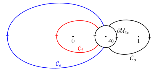
Refer to caption
Figure 4.6: The contour ฮฃR=๐’žiโˆช๐’žeโˆช๐’žoโˆชโˆ‚๐’ฐz0subscriptฮฃ๐‘…subscript๐’ž๐‘–subscript๐’ž๐‘’subscript๐’ž๐‘œsubscript๐’ฐsubscript๐‘ง0\Sigma_{R}=\mathcal{C}_{i}\cup\mathcal{C}_{e}\cup\mathcal{C}_{o}\cup\partial{\cal U}_{z_{0}} where ๐’ži,๐’žesubscript๐’ž๐‘–subscript๐’ž๐‘’\mathcal{C}_{i},\mathcal{C}_{e} and ๐’žosubscript๐’ž๐‘œ\mathcal{C}_{o} are defined only in โ„‚\๐’ฐz0\โ„‚subscript๐’ฐsubscript๐‘ง0\mathbb{C}\backslash{\cal U}_{z_{0}}.

We now define the error matrix R๐‘…R in two regions of the plane, using our approximations to the matrix T๐‘‡T. Set

Rโ€‹(z)={Tโ€‹(z)โ€‹(P^(0)โ€‹(z))โˆ’1,zโˆˆ๐’ฐz0,Tโ€‹(z)โ€‹(P^โˆžโ€‹(z))โˆ’1,zโˆˆโ„‚โˆ–๐’ฐz0.๐‘…๐‘งcases๐‘‡๐‘งsuperscriptsuperscript^๐‘ƒ0๐‘ง1๐‘งsubscript๐’ฐsubscript๐‘ง0๐‘‡๐‘งsuperscriptsuperscript^๐‘ƒ๐‘ง1๐‘งโ„‚subscript๐’ฐsubscript๐‘ง0R(z)=\begin{cases}T(z)\left(\hat{P}^{(0)}(z)\right)^{-1},&z\in\mathcal{U}_{z_{0}}\ ,\\ T(z)\left(\hat{P}^{\infty}(z)\right)^{-1},&z\in\mathbb{C}\setminus\mathcal{U}_{z_{0}}.\end{cases} (4.56)

The matrix R๐‘…R is piecewise analytic in โ„‚โ„‚\mathbb{C} with a jump across ฮฃRsubscriptฮฃ๐‘…\Sigma_{R} (see Fig.ย 4.6).
Riemannโ€“Hilbert problem for R๐‘…R

  1. 1.

    R๐‘…R is analytic in โ„‚โˆ–ฮฃRโ„‚subscriptฮฃ๐‘…\mathbb{C}\setminus\Sigma_{R},

  2. 2.

    For zโˆˆฮฃR๐‘งsubscriptฮฃ๐‘…z\in\Sigma_{R}, we have

    R+โ€‹(z)=Rโˆ’โ€‹(z)โ€‹vRโ€‹(z),subscript๐‘…๐‘งsubscript๐‘…๐‘งsubscript๐‘ฃ๐‘…๐‘งR_{+}(z)=R_{-}(z)v_{R}(z), (4.57)

    with

    vR(z)={P^โˆ’โˆžโ€‹(z)โ€‹vTโ€‹(z)โ€‹(P^+โˆžโ€‹(z))โˆ’1zโˆˆฮฃR\โˆ‚๐’ฐz0P^โˆžโ€‹(z)โ€‹(P^(0)โ€‹(z))โˆ’1zโˆˆโˆ‚๐’ฐz0v_{R}(z)=\left\{\begin{split}\hat{P}^{\infty}_{-}(z)v_{T}(z)\left(\hat{P}_{+}^{\infty}(z)\right)^{-1}&\quad z\in\Sigma_{R}\backslash\partial\mathcal{U}_{z_{0}}\\ \hat{P}^{\infty}(z)\left(\hat{P}^{(0)}(z)\right)^{-1}&\quad z\in\partial\mathcal{U}_{z_{0}}\end{split}\right. (4.58)
  3. 3.

    As zโ†’โˆžโ†’๐‘งz\to\infty, we have

    Rโ€‹(z)=I+๐’ชโ€‹(zโˆ’1).๐‘…๐‘ง๐ผ๐’ชsuperscript๐‘ง1R(z)=I+{\mathcal{O}}\left(z^{-1}\right). (4.59)

The jump matrices across the contour ฮฃR\โˆ‚๐’ฐz0\subscriptฮฃ๐‘…subscript๐’ฐsubscript๐‘ง0\Sigma_{R}\backslash\partial\mathcal{U}_{z_{0}} are all exponentially close to I๐ผI for large k๐‘˜k because vTโ€‹(z)subscript๐‘ฃ๐‘‡๐‘งv_{T}(z) converges exponentially fast to vโˆžโ€‹(z)superscript๐‘ฃ๐‘งv^{\infty}(z) defined in (4.16) for zโˆˆโ„‚\๐’ฐz0๐‘ง\โ„‚subscript๐’ฐsubscript๐‘ง0z\in\mathbb{C}\backslash{\cal U}_{z_{0}} and the product

P^โˆ’โˆžโ€‹(z)โ€‹vโˆžโ€‹(z)โ€‹(P^+โˆžโ€‹(z))โˆ’1=(I+Czโˆ’z0)โ€‹Pโˆ’โˆžโ€‹(z)โ€‹vโˆžโ€‹(z)โ€‹(P+โˆžโ€‹(z))โˆ’1โ€‹(I+Czโˆ’z0)โˆ’1=Isubscriptsuperscript^๐‘ƒ๐‘งsuperscript๐‘ฃ๐‘งsuperscriptsuperscriptsubscript^๐‘ƒ๐‘ง1๐ผ๐ถ๐‘งsubscript๐‘ง0subscriptsuperscript๐‘ƒ๐‘งsuperscript๐‘ฃ๐‘งsuperscriptsuperscriptsubscript๐‘ƒ๐‘ง1superscript๐ผ๐ถ๐‘งsubscript๐‘ง01๐ผ\hat{P}^{\infty}_{-}(z)v^{\infty}(z)\left(\hat{P}_{+}^{\infty}(z)\right)^{-1}=\left(I+\frac{C}{z-z_{0}}\right)P^{\infty}_{-}(z)v^{\infty}(z)\left(P_{+}^{\infty}(z)\right)^{-1}\left(I+\frac{C}{z-z_{0}}\right)^{-1}=I

with Pโˆžโ€‹(z)superscript๐‘ƒ๐‘งP^{\infty}(z) defined in (4.25) and C๐ถC in (4.53). The only jump that is not exponentially small is the one on โˆ‚๐’ฐz0subscript๐’ฐsubscript๐‘ง0\partial\mathcal{U}_{z_{0}}. Indeed one has from (4.55)

vRโ€‹(z)=P^โˆžโ€‹(z)โ€‹(P^0โ€‹(z))โˆ’1=I+ฮณโ€‹eโ€‹(z)22โ€‹k12+ฮณโ€‹wโ€‹(z)โ€‹ฮฒ21โ€‹(cโ€‹kฮณโˆ’12zโˆ’z0โˆ’1c2โ€‹k2โ€‹ฮณโˆ’1(zโˆ’z0)2โˆ’cโ€‹kฮณโˆ’12zโˆ’z0)+ฮณโ€‹(1โˆ’ฮณ)4โ€‹kโ€‹wโ€‹(z)2โ€‹(102โ€‹cโ€‹kฮณโˆ’12(zโˆ’z0)โˆ’1)+1k32โˆ’ฮณโ€‹wโ€‹(z)3โ€‹(๐’ชโ€‹(kโˆ’12โˆ’ฮณ)๐’ชโ€‹(kโˆ’2โ€‹ฮณ)ฮณโ€‹(1โˆ’ฮณ)4โ€‹ฮฒ12โ€‹eโ€‹(z)2+๐’ชโ€‹(kโˆ’1)๐’ชโ€‹(kโˆ’12โˆ’ฮณ))+๐’ชโ€‹(kโˆ’2,kฮณโˆ’52)subscript๐‘ฃ๐‘…๐‘งsuperscript^๐‘ƒ๐‘งsuperscriptsuperscript^๐‘ƒ0๐‘ง1๐ผ๐›พ๐‘’superscript๐‘ง22superscript๐‘˜12๐›พ๐‘ค๐‘งsubscript๐›ฝ21matrix๐‘superscript๐‘˜๐›พ12๐‘งsubscript๐‘ง01superscript๐‘2superscript๐‘˜2๐›พ1superscript๐‘งsubscript๐‘ง02๐‘superscript๐‘˜๐›พ12๐‘งsubscript๐‘ง0๐›พ1๐›พ4๐‘˜๐‘คsuperscript๐‘ง2matrix102๐‘superscript๐‘˜๐›พ12๐‘งsubscript๐‘ง011superscript๐‘˜32๐›พ๐‘คsuperscript๐‘ง3matrix๐’ชsuperscript๐‘˜12๐›พ๐’ชsuperscript๐‘˜2๐›พ๐›พ1๐›พ4subscript๐›ฝ12๐‘’superscript๐‘ง2๐’ชsuperscript๐‘˜1๐’ชsuperscript๐‘˜12๐›พ๐’ชsuperscript๐‘˜2superscript๐‘˜๐›พ52\begin{split}v_{R}(z)=\hat{P}^{\infty}(z)(\hat{P}^{0}(z))^{-1}&=I+\dfrac{\gamma e(z)^{2}}{2k^{\frac{1}{2}+\gamma}w(z)\beta_{21}}\begin{pmatrix}\dfrac{ck^{\gamma-\frac{1}{2}}}{z-z_{0}}&-1\\ \dfrac{c^{2}k^{2\gamma-1}}{(z-z_{0})^{2}}&-\dfrac{ck^{\gamma-\frac{1}{2}}}{z-z_{0}}\end{pmatrix}+\dfrac{\gamma(1-\gamma)}{4kw(z)^{2}}\begin{pmatrix}1&0\\ \dfrac{2ck^{\gamma-\frac{1}{2}}}{(z-z_{0})}&-1\end{pmatrix}\\ &+\dfrac{1}{k^{\frac{3}{2}-\gamma}w(z)^{3}}\begin{pmatrix}{\mathcal{O}}\left(k^{-\frac{1}{2}-\gamma}\right)&{\mathcal{O}}\left(k^{-2\gamma}\right)\\ \dfrac{\gamma(1-\gamma)}{4\beta_{12}e(z)^{2}}+{\mathcal{O}}\left(k^{-1}\right)&{\mathcal{O}}\left(k^{-\frac{1}{2}-\gamma}\right)\end{pmatrix}+{\mathcal{O}}\left(k^{-2},k^{\gamma-\frac{5}{2}}\right)\end{split} (4.60)

where

eโ€‹(z)=E11โ€‹(z)โ€‹kฮณ/2๐‘’๐‘งsubscript๐ธ11๐‘งsuperscript๐‘˜๐›พ2e(z)=E_{11}(z)k^{\gamma/2} (4.61)

and we have substituted the explicit expressions of the matrix ฮจ1subscriptฮจ1\Psi_{1}, ฮจ2subscriptฮจ2\Psi_{2} and ฮจ3subscriptฮจ3\Psi_{3} as given by (4.43).

We have the following two cases depending on the value of ฮณโˆˆ(0,1)๐›พ01\gamma\in(0,1).

  • (a)

    0<ฮณ<120๐›พ120<\gamma<\frac{1}{2}

    vRโ€‹(z)=P^โˆžโ€‹(z)โ€‹(P^0โ€‹(z))โˆ’1=I+vR1โ€‹(z)k12+ฮณ+๐’ชโ€‹(kโˆ’1),subscript๐‘ฃ๐‘…๐‘งsuperscript^๐‘ƒ๐‘งsuperscriptsuperscript^๐‘ƒ0๐‘ง1๐ผsuperscriptsubscript๐‘ฃ๐‘…1๐‘งsuperscript๐‘˜12๐›พ๐’ชsuperscript๐‘˜1v_{R}(z)=\hat{P}^{\infty}(z)(\hat{P}^{0}(z))^{-1}=I+\dfrac{v_{R}^{1}(z)}{k^{\frac{1}{2}+\gamma}}+{\mathcal{O}}\left(k^{-1}\right), (4.62)

    where

    vR1โ€‹(z)=โˆ’ฮณโ€‹eโ€‹(z)22โ€‹wโ€‹(z)โ€‹ฮฒ21โ€‹(0100)superscriptsubscript๐‘ฃ๐‘…1๐‘ง๐›พ๐‘’superscript๐‘ง22๐‘ค๐‘งsubscript๐›ฝ21matrix0100v_{R}^{1}(z)=-\dfrac{\gamma e(z)^{2}}{2w(z)\beta_{21}}\begin{pmatrix}0&1\\ 0&0\end{pmatrix} (4.63)
  • (b)

    12โ‰คฮณ<112๐›พ1\frac{1}{2}\leq\gamma<1

    vRโ€‹(z)=P^โˆžโ€‹(z)โ€‹(P^0โ€‹(z))โˆ’1=I+vR(1)โ€‹(z)k32โˆ’ฮณ+vR(2)โ€‹(z)k+vR(3)โ€‹(z)k12+ฮณ+๐’ชโ€‹(kฮณโˆ’52).subscript๐‘ฃ๐‘…๐‘งsuperscript^๐‘ƒ๐‘งsuperscriptsuperscript^๐‘ƒ0๐‘ง1๐ผsuperscriptsubscript๐‘ฃ๐‘…1๐‘งsuperscript๐‘˜32๐›พsuperscriptsubscript๐‘ฃ๐‘…2๐‘ง๐‘˜superscriptsubscript๐‘ฃ๐‘…3๐‘งsuperscript๐‘˜12๐›พ๐’ชsuperscript๐‘˜๐›พ52\begin{split}v_{R}(z)=\hat{P}^{\infty}(z)(\hat{P}^{0}(z))^{-1}&=I+\dfrac{v_{R}^{(1)}(z)}{k^{\frac{3}{2}-\gamma}}+\dfrac{v_{R}^{(2)}(z)}{k}+\dfrac{v_{R}^{(3)}(z)}{k^{\frac{1}{2}+\gamma}}+{\mathcal{O}}\left(k^{\gamma-\frac{5}{2}}\right).\end{split} (4.64)

    where

    vR(1)โ€‹(z)=(c2ฮฒ21โ€‹wโ€‹(z)โ€‹eโ€‹(z)2(zโˆ’z0)2+cโ€‹(1โˆ’ฮณ)2โ€‹wโ€‹(z)2โ€‹(zโˆ’z0)+(1โˆ’ฮณ)2โ€‹ฮฒ12โ€‹wโ€‹(z)3โ€‹eโ€‹(z)2)โ€‹(0010)vR(2)โ€‹(z)=(ฮณโ€‹c2โ€‹ฮฒ21โ€‹eโ€‹(z)2wโ€‹(z)โ€‹(zโˆ’z0)+ฮณโ€‹(1โˆ’ฮณ)4โ€‹wโ€‹(z)2)โ€‹ฯƒ3vR(3)โ€‹(z)=โˆ’ฮณโ€‹eโ€‹(z)22โ€‹wโ€‹(z)โ€‹ฮฒ21โ€‹(0100),superscriptsubscript๐‘ฃ๐‘…1๐‘งsuperscript๐‘2subscript๐›ฝ21๐‘ค๐‘ง๐‘’superscript๐‘ง2superscript๐‘งsubscript๐‘ง02๐‘1๐›พ2๐‘คsuperscript๐‘ง2๐‘งsubscript๐‘ง01๐›พ2subscript๐›ฝ12๐‘คsuperscript๐‘ง3๐‘’superscript๐‘ง2matrix0010superscriptsubscript๐‘ฃ๐‘…2๐‘ง๐›พ๐‘2subscript๐›ฝ21๐‘’superscript๐‘ง2๐‘ค๐‘ง๐‘งsubscript๐‘ง0๐›พ1๐›พ4๐‘คsuperscript๐‘ง2subscript๐œŽ3superscriptsubscript๐‘ฃ๐‘…3๐‘ง๐›พ๐‘’superscript๐‘ง22๐‘ค๐‘งsubscript๐›ฝ21matrix0100\begin{split}v_{R}^{(1)}(z)&=\left(\dfrac{c^{2}}{\beta_{21}}\dfrac{w(z)e(z)^{2}}{(z-z_{0})^{2}}+\dfrac{c(1-\gamma)}{2w(z)^{2}(z-z_{0})}+\dfrac{(1-\gamma)}{2\beta_{12}w(z)^{3}e(z)^{2}}\right)\begin{pmatrix}0&0\\ 1&0\end{pmatrix}\\ v_{R}^{(2)}(z)&=\left(\dfrac{\gamma c}{2\beta_{21}}\dfrac{e(z)^{2}}{w(z)(z-z_{0})}+\dfrac{\gamma(1-\gamma)}{4w(z)^{2}}\right)\sigma_{3}\\ v_{R}^{(3)}(z)&=-\dfrac{\gamma e(z)^{2}}{2w(z)\beta_{21}}\begin{pmatrix}0&1\\ 0&0\end{pmatrix},\end{split} (4.65)

By the standard theory of small norm Riemannโ€“Hilbert problems one has a similar expansion for Rโ€‹(z)๐‘…๐‘งR(z) in the large k๐‘˜k limit.

Case (a): 0<ฮณ<120๐›พ120<\gamma<\frac{1}{2}

Rโ€‹(z)=I+R(1)k12+ฮณ+๐’ชโ€‹(kโˆ’1)๐‘…๐‘ง๐ผsuperscript๐‘…1superscript๐‘˜12๐›พ๐’ชsuperscript๐‘˜1R(z)=I+\dfrac{R^{(1)}}{k^{\frac{1}{2}+\gamma}}+{\mathcal{O}}\left(k^{-1}\right) (4.66)

Compatibility of (4.57), (4.62) and (4.66) and the jump condition R+=Rโˆ’โ€‹v^Rsubscript๐‘…subscript๐‘…subscript^๐‘ฃ๐‘…R_{+}=R_{-}\hat{v}_{R} on โˆ‚๐’ฐz0subscript๐’ฐsubscript๐‘ง0\partial\mathcal{U}_{z_{0}} gives the following relations.

R+(1)โ€‹(z)=Rโˆ’(1)โ€‹(z)+vR(1)โ€‹(z),zโˆˆโˆ‚๐’ฐz0formulae-sequencesubscriptsuperscript๐‘…1๐‘งsubscriptsuperscript๐‘…1๐‘งsubscriptsuperscript๐‘ฃ1๐‘…๐‘ง๐‘งsubscript๐’ฐsubscript๐‘ง0R^{(1)}_{+}(z)=R^{(1)}_{-}(z)+v^{(1)}_{R}(z),\quad z\in\partial\mathcal{U}_{z_{0}} (4.67)

with vR(1)โ€‹(z)subscriptsuperscript๐‘ฃ1๐‘…๐‘งv^{(1)}_{R}(z) defined in (4.63). In addition R(1)โ€‹(z)superscript๐‘…1๐‘งR^{(1)}(z) is analytic in โ„‚\โˆ‚๐’ฐz0\โ„‚subscript๐’ฐsubscript๐‘ง0\mathbb{C}\backslash\partial\mathcal{U}_{z_{0}} and R(1)โ€‹(โˆž)=0superscript๐‘…10R^{(1)}(\infty)=0. The unique function that satisfies those conditions is given by

R(1)โ€‹(z)=12โ€‹ฯ€โ€‹iโ€‹โˆฎvR(1)โ€‹(ฮพ)ฮพโˆ’zโ€‹๐‘‘ฮพ={1zโˆ’z0โ€‹ฮณโ€‹eโ€‹(z0)22โ€‹wโ€ฒโ€‹(z0)โ€‹ฮฒ21โ€‹(0100)zโˆˆโ„‚\๐’ฐz0vR(1)โ€‹(z)+1zโˆ’z0โ€‹ฮณโ€‹eโ€‹(z0)22โ€‹wโ€ฒโ€‹(z0)โ€‹ฮฒ21โ€‹(0100)zโˆˆ๐’ฐz0,superscript๐‘…1๐‘ง12๐œ‹๐‘–contour-integralsubscriptsuperscript๐‘ฃ1๐‘…๐œ‰๐œ‰๐‘งdifferential-d๐œ‰cases1๐‘งsubscript๐‘ง0๐›พ๐‘’superscriptsubscript๐‘ง022superscript๐‘คโ€ฒsubscript๐‘ง0subscript๐›ฝ21matrix0100๐‘ง\โ„‚subscript๐’ฐsubscript๐‘ง0missing-subexpressionmissing-subexpressionsubscriptsuperscript๐‘ฃ1๐‘…๐‘ง1๐‘งsubscript๐‘ง0๐›พ๐‘’superscriptsubscript๐‘ง022superscript๐‘คโ€ฒsubscript๐‘ง0subscript๐›ฝ21matrix0100๐‘งsubscript๐’ฐsubscript๐‘ง0R^{(1)}(z)=\dfrac{1}{2\pi i}\oint\dfrac{v^{(1)}_{R}(\xi)}{\xi-z}d\xi=\left\{\begin{array}[]{ll}\dfrac{1}{z-z_{0}}\dfrac{\gamma e(z_{0})^{2}}{2w^{\prime}(z_{0})\beta_{21}}\begin{pmatrix}0&1\\ 0&0\end{pmatrix}&z\in\mathbb{C}\,\backslash\,\mathcal{U}_{z_{0}}\\ &\\ v^{(1)}_{R}(z)+\dfrac{1}{z-z_{0}}\dfrac{\gamma e(z_{0})^{2}}{2w^{\prime}(z_{0})\beta_{21}}\begin{pmatrix}0&1\\ 0&0\end{pmatrix}&z\in\mathcal{U}_{z_{0}},\end{array}\right. (4.68)

where the integral is taken along โˆ‚๐’ฐz0subscript๐’ฐsubscript๐‘ง0\partial{\cal U}_{z_{0}}. Using the definition of ฮฒ21subscript๐›ฝ21\beta_{21} , wโ€ฒโ€‹(z)superscript๐‘คโ€ฒ๐‘งw^{\prime}(z) and eโ€‹(z)๐‘’๐‘งe(z) given in (4.41), (4.46) and (4.61) respectively one has

R(1)โ€‹(z)={1zโˆ’z0โ€‹ฮณโ€‹z02cโ€‹(0100)zโˆˆโ„‚\๐’ฐz0vR(1)โ€‹(z)+1zโˆ’z0โ€‹ฮณโ€‹z02cโ€‹(0100)zโˆˆ๐’ฐz0,superscript๐‘…1๐‘งcases1๐‘งsubscript๐‘ง0๐›พsuperscriptsubscript๐‘ง02๐‘matrix0100๐‘ง\โ„‚subscript๐’ฐsubscript๐‘ง0missing-subexpressionmissing-subexpressionsubscriptsuperscript๐‘ฃ1๐‘…๐‘ง1๐‘งsubscript๐‘ง0๐›พsuperscriptsubscript๐‘ง02๐‘matrix0100๐‘งsubscript๐’ฐsubscript๐‘ง0R^{(1)}(z)=\left\{\begin{array}[]{ll}\dfrac{1}{z-z_{0}}\dfrac{\gamma z_{0}^{2}}{c}\begin{pmatrix}0&1\\ 0&0\end{pmatrix}&z\in\mathbb{C}\,\backslash\,\mathcal{U}_{z_{0}}\\ &\\ v^{(1)}_{R}(z)+\dfrac{1}{z-z_{0}}\dfrac{\gamma z_{0}^{2}}{c}\begin{pmatrix}0&1\\ 0&0\end{pmatrix}&z\in\mathcal{U}_{z_{0}},\end{array}\right. (4.69)

with the constant c๐‘c defined in (4.54).

Case (b):