A Class of Parallel Decomposition Algorithms for SVMs Training

Abstract

The training of Support Vector Machines may be a very difficult task when dealing with very large datasets. The memory requirement and the time consumption of the SVMs algorithms grow rapidly with the increase of the data. To overcome these drawbacks, we propose a parallel decomposition algorithmic scheme for SVMs training for which we prove global convergence under suitable conditions. We outline how these assumptions can be satisfied in practice and we suggest various specific implementations exploiting the adaptable structure of the algorithmic model.

Keywords. Decomposition Algorithm, Big Data, Support Vector Machine, Machine Learning, Parallel Computing

1 Introduction

A Support Vector Machine (SVM) is a well known classification and regression tool that has spread in many scientific fields during the last two decades, see [5]. Given a training set of $n$ input-target pairs

$$D=\{({\bf z}_{r},y_{r}),\;r=1,\dots,n,\;{\bf z}_{r}\in{\mathbb{R}}^{m},\;y_{r}\in\{-1,1\}\},$$

an SVM provides a prediction model used to classify new unlabeled samples.
The dual formulation of an SVM training problem is

$$\displaystyle\min_{{\bf x}}\; f({\bf x}):=\frac{1}{2}{\bf x}^{\scriptscriptstyle T}Q{\bf x}-{\bf e}^{\scriptscriptstyle T}{\bf x}$$

$${\bf y}^{\scriptscriptstyle T}{\bf x}=0$$ (1)

$$\mathbf{0}\leq{\bf x}\leq C{\bf e},$$

where ${\bf x}\in{\mathbb{R}}^{n}$, ${\bf e}\in{\mathbb{R}}^{n}$ is a vector of all ones, $C>0$ is a positive constant, ${\bf y}\in\{-1,1\}^{n}$ and $Q$ is an $n\times n$ symmetric positive semidefinte matrix. Each component of ${\bf x}$ is associated with a sample of the training set and ${\bf y}$ is the vector of the corresponding labels. Entries of $Q$ are defined by

$$Q_{rq}=y_{r}y_{q}K({\bf z}_{r},{\bf z}_{q}),\quad\quad r,q=1,2,\dots,n,$$

where $K:{\mathbb{R}}^{m}\times{\mathbb{R}}^{m}\to{\mathbb{R}}$ is a given kernel function [23].
Many real SVM applications are characterized by a large dimensional training set. This implies that hessian matrix $Q$ is so big that it cannot be entirely stored in memory. For this reason classical optimization algorithms that use first and second order information cannot be used to efficiently solve problem (1).
To overcome this difficulty, many decomposition algorithms have been proposed in literature. At each iteration, they split the original problem into a sequence of smaller subproblems where only a subset of variables (working set) are updated. Columns of the hessian submatrix corresponding to each subproblem are, partially or entirely, recomputed at each step. These strategies can be mainly divided into SMO (Sequential Minimal Optimization) and non-SMO methods. SMO algorithms (see e.g. [3, 21]) work with subproblems of dimension two, so that their solutions can be computed analytically; while non-SMO algorithms (see e.g. [10, 13]) need an iterative optimization method to solve each subproblem. From the theoretical point of view, the policy for updating the working set plays a crucial role to prove convergence. In case of SMO methods, a proper selection rule based on the maximal violating principle is sufficient to ensure asymptotic convergence of the decomposition scheme [4, 16]. For larger working sets, convergence proofs are available under further conditions [15, 19, 20].

In recent years SVMs have been applied to huge datasets, mainly related to web-oriented applications. To reduce the big amount of time needed for the training of SVMs on such huge datasets, parallel algorithms have been proposed. Some of these parallel approaches to SVMs consists in distributing the most expensive tasks, such as subproblems solving and gradient updating, among the available processors, see [11, 26, 27]. Another way of fruitfully exploit parallelism is based on splitting the training data into subsets and distributing them among the processors [2, 28]. Among these parallel techniques, there are also the so called Cascade-SVM (see [12, 25]) that has been introduced to face big dimensional instances. While achieving a good reduction of the training time respect to sequential methods, these methods may lack convergence properties or may require strong assumptions to prove it.

Actually, combining decomposition rules, for the selection of working sets, and parallelism makes the proof of convergence a very difficult task, see [18]. This is mainly due to nonseparability of the feasible set of problem (1).

In this work we propose a class of convergent parallel training algorithms based on the decomposition of problem (1) into a partition of subproblems that can be solved independently by parallel processes. The convergence to a global optimum of problem (1) is proved under realistic assumptions. It partially exploits results introduced in [9, 24]. The algorithmic framework presented may include, as a special case, other convergent theoretical models like [18].

The paper is organized as follows: in Section 2 we introduce some preliminary results; in Section 3 we introduce a general parallel algorithmic scheme. We analyze its convergence properties in Sections 4, 5 and 6; in Section 7 we discuss about some possible practical implementations.

Notation

In the following we use this notation. Vectors are boldface. Given a vector $\mathbf{x}\in{\mathbb{R}}^{n}$ with components $x_{r}$ and a subset of indices $P\subseteq\{1,\dots,n\}$ we denote by $\mathbf{x}_{P}\in{\mathbb{R}}^{|P|}$ the subvector made up of components $x_{r}$ with $r\in P$ and by $\mathbf{x}_{-P}\in{\mathbb{R}}^{n-|P|}$ the subvector made up of components $x_{r}$ with $r\not\in P$. By $\|\cdot\|$ we indicate the euclidean norm, whereas the zero norm of a vector $\|\mathbf{x}\|_{0}$ denotes the number of nonzero components of vector $\mathbf{x}$. Further given a square $n\times n$ matrix ${Q}$, we denote by ${Q}_{*r}$ the $r-$th column of the matrix. Given two subsets of indices $P_{r},P_{q}\subseteq\{1,\dots,n\}$, we write $Q_{P_{r}P_{q}}$ to indicate the $|P_{r}|\times|P_{q}|$ submatrix of $Q$ with row indices in block $P_{r}$ and column indices in block $P_{q}$. We denote by $\lambda_{\min}^{Q}$ and $\lambda_{\max}^{Q}$ respectively the minimum and maximum eigenvalue of a square matrix $Q$. For the sake of simplicity we denote the $r-$th component of the gradient as $\nabla f(\mathbf{x})_{r}=\frac{\partial f(\mathbf{x})}{\partial x_{r}}$ and as $\nabla_{P}f(\mathbf{x})\in{\mathbb{R}}^{|P|}$ the subvector of the gradient made up of components $\frac{\partial f(\mathbf{x})}{\partial x_{r}}$ with $r\in P$. We denote by $\cal F$ the feasible set of problem (1), namely

$${\cal F}=\{\mathbf{x}\in{\mathbb{R}}^{n}:{\bf y}^{\scriptscriptstyle T}{\bf x}=0,\ \ \mathbf{0}\leq{\bf x}\leq C{\bf e}\}.$$

Note that all the results that we report in the sequel hold also in the case of feasible set ${\cal F}=\{\mathbf{x}\in{\mathbb{R}}^{n}:{\bf y}^{\scriptscriptstyle T}{\bf x}=b,\ \ \mathbf{0}\leq{\bf x}\leq C{\bf e}\},$ where $\mathbf{y}\in{\mathbb{R}}^{n}$ and $b\in{\mathbb{R}}$, but for sake of simplicity we refer to the case $b=0$ and $\mathbf{y}\in\{-1,1\}^{n}$.

2 Optimality Conditions and Preliminary Results

Let us consider a solution ${\bf x}^{*}$ of problem (1). Since constraints are linear and the objective function is convex, necessary and sufficient conditions for optimality are the Karush-Kuhn-Tucker (KKT) conditions that state that there exists a scalar $s$ such that for all indices $r\in\{1,\ldots,n\}$:

$$\nabla f({\bf x}^{*})_{r}+sy_{r}\geq 0\quad\mbox{if} \ x^{*}_{r}=0$$

$$\nabla f({\bf x}^{*})_{r}+sy_{r}\leq 0\quad\mbox{if} \ x^{*}_{r}=C$$ (2)

$$\nabla f({\bf x}^{*})_{r}+sy_{r}=0\quad\mbox{if} \ 0<\ x^{*}_{r}<C.$$

It is well known (see e.g.[13]) that KKT conditions can be written in a more compact form by introducing the following sets

$$I_{up}({\bf x}):=\{r\subseteq\{1,\dots,n\}:\ x_{r}<C,\ y_{r}=1,\mbox{ or }x_{r}>0,\ y_{r}=-1\},$$

$$I_{low}({\bf x}):=\{r\subseteq\{1,\dots,n\}:\ x_{r}<C,\ y_{r}=-1,\mbox{ or }x_{r}>0,\ y_{r}=1\}.$$

Assuming that $I_{up}({\bf x}^{*})\neq\emptyset$ and $I_{low}({\bf x}^{*})\neq\emptyset$, then we can rewrite (2) as

$$m({\bf x}^{*})=\max_{r\in I_{up}({\bf x}^{*})}-\frac{\nabla f({\bf x}^{*})_{r}}{y_{r}}\leq\min_{r\in I_{low}({\bf x}^{*})}-\frac{\nabla f({\bf x}^{*})_{r}}{y_{r}}=M({\bf x}^{*}).$$ (3)

By the convexity of problem (1), we can say that ${\bf x}^{*}$ is optimal if and only if either $I_{up}({\bf x}^{*})=\emptyset$ or $I_{low}({\bf x}^{*})=\emptyset$ or condition (3) holds.

Such a form of the KKT conditions is the basis of most efficient sequential decomposition algorithms for the solution of problem (1). In decomposition algorithms the sequence $\{{\bf x}^{k}\}$ is obtained by changing at each iteration only a subset of the variables, let’s say ${\bf x}_{P_{i}}$ with $P_{i}\subset\{1,\ldots,n\}$, whilst the other ${\bf x}_{-P_{i}}$ remain unchanged. Thus the sequence takes the form

$$\mathbf{x}^{k+1}=\mathbf{x}^{k}+\alpha^{k}\mathbf{d}^{k},$$

where $\mathbf{d}^{k}$ is a sparse feasible descent direction such that $\|\mathbf{d}^{k}\|_{0}=|P_{i}|$ with $|P_{i}|<<n$ and $\alpha^{k}$ represents a stepsize along this direction. Whatever the feasible direction $\mathbf{d}^{k}$ is, since the objective function is quadratic and convex, the choice of the stepsize can be performed by using an exact minimization of the objective function along $\mathbf{d}^{k}$. Indeed, let $\bar{\beta}>0$ be the largest feasible step at $\mathbf{x}^{k}\in{\cal F}$ along the descent direction $\mathbf{d}^{k}$ then

$$\alpha^{k}:=\min\left\{-\frac{\nabla{f}(\mathbf{x}^{k})^{\scriptscriptstyle T}\mathbf{d}^{k}}{{\mathbf{d}^{k}}^{\scriptscriptstyle T}{Q}\mathbf{d}^{k}},\,\bar{\beta}\right\}.$$ (4)

Sequential decomposition methods differ in the choice of the direction $\mathbf{d}^{k}$, or equivalently in the choice of the so called working set $P_{i}$.

Sequential Minimal Optimization (SMO) methods uses feasible descent directions $\mathbf{d}^{k}$ with $\|\mathbf{d}^{k}\|_{0}=2$ which is the minimal possible cardinality due to the equality constraint. In a feasible point ${{\bf x}}\in{\cal F}$ a feasible direction with two nonzero components $\mathbf{d}^{(ij)}$ is given by

$$d^{(ij)}_{r}:=\begin{cases}\displaystyle\ \ \frac{1}{y_{r}}&\mbox{ if }r=i\\[8.00003pt] \displaystyle-\frac{1}{y_{r}}&\mbox{ if }r=j\\[8.00003pt] \quad 0&\mbox{ otherwise}\end{cases},\quad r=1,\ldots,n.$$ (5)

for any pair $(i,j)\in I_{up}(\mathbf{x})\times I_{low}(\mathbf{x})$. We say that a pair $(i,j)\in I_{up}(\mathbf{x})\times I_{low}(\mathbf{x})$ is a violating pair at $\mathbf{x}$ if it satisfied also $\nabla f(\mathbf{x})^{T}\mathbf{d}^{(ij)}<0$.

The exact optimal stepsize $\alpha\geq 0$ along a direction $\mathbf{d}^{(ij)}$ can be efficiently computed by noting that in (4) we have

$$\bar{\beta}=\min\left\{\beta_{i},\,\beta_{j}\right\},$$ (6)

where

$$\beta_{h}:=\left\{\begin{array}[]{ll}x_{h}&\text{ if }d^{(ij)}_{h}<0\\ C-x_{h}&\text{ if }d^{(ij)}_{h}>0.\end{array}\right.$$ (7)

Thus we get the value of the optimal stepsize $\alpha$ along a direction $\mathbf{d}^{(ij)}$ as

$$\alpha:=\min\left\{-\frac{\nabla{f}_{i}y_{i}-\nabla{f}_{j}y_{j}}{Q_{ii}+Q_{jj}-2y_{i}y_{j}Q_{ij}},\,\bar{\beta}\right\}.$$ (8)

Among such minimal descent directions, i.e. violating pairs, a crucial role is played by the so called Most Violating Pair (MVP) direction (see e.g. [13]). To be more specific, given a feasible point ${{\bf x}}$, let us define the sets

$$I_{up}^{MVP}({{\bf x}}):=\left\{i\in I_{up}(\mathbf{x}):~{}i\in\arg\!\!\!\max_{h\in I_{up}({{\bf x}})}-\frac{\nabla f({{\bf x}})_{h}}{y_{h}}\right\},$$

$$I_{low}^{MVP}({{\bf x}}):=\left\{j\in I_{low}(\mathbf{x}):~{}j\in\arg\!\!\!\min_{h\in{I_{low}}({{\bf x}})}-\frac{\nabla f({{\bf x}})_{h}}{y_{h}}\right\}.$$

If $\mathbf{x}$ is not a solution of problem (1), then $(i_{\texttt{MVP}},j_{\texttt{MVP}})\in I_{up}^{MVP}({\bf x})\times I_{low}^{MVP}({\bf x})$ is a pair, possibly not unique, that violates the KKT conditions at most and it is said Most Violating Pair (MVP). In the sequel, for the sake of notational simplicity, we assume that, for every feasible $\mathbf{x}$, the MVP is unique as this makes no difference in our analysis.
The direction $\mathbf{d}_{\texttt{MVP}}\in{\mathbb{R}}^{n}$ corresponding to the pair $(i_{\texttt{MVP}},j_{\texttt{MVP}})\in I_{up}^{MVP}({\bf x})\times I_{low}^{MVP}({\bf x})$ is, among all feasible descent directions with only two nonzero components, the steepest descent one at $\mathbf{x}$.
Now we are ready to introduce the definition of “most violating step”. Let $\mathbf{x}_{\texttt{MVP}}=\mathbf{x}+\alpha_{\texttt{MVP}}\mathbf{d}_{\texttt{MVP}}$ with $\alpha_{\texttt{MVP}}$ obtained by (8) with $i=i_{\texttt{MVP}}$, $j=j_{\texttt{MVP}}$.

Definition 1 (Most Violating Step)

At a point $\mathbf{x}\in{\cal F}$, we define the “Most Violating Step” (MVS) $S_{\texttt{MVP}}$ as:

$$S_{\texttt{MVP}}(\mathbf{x}):=\|\mathbf{x}_{\texttt{MVP}}-\mathbf{x}\|=|\alpha_{\texttt{MVP}}|\|\mathbf{d}_{\texttt{MVP}}\|.$$ (9)

In particular, since $y^{i}\in\{-1,1\}$ we have that $S_{\texttt{MVP}}(\mathbf{x})=|\alpha_{\texttt{MVP}}|\sqrt{2}$.

We can state the optimality condition using the definition of MVS.

Proposition 1

A point ${\bf x}^{*}\in\cal F$ is optimal for problem (1) if and only if either $I_{up}({\bf x}^{*})=\emptyset$ or $I_{low}({\bf x}^{*})=\emptyset$ or $S_{\texttt{MVP}}({\bf x}^{*})=0$.

Proof. 1

As said above ${\bf x}^{*}$ is optimal for problem (1) if and only if either $I_{up}({\bf x}^{*})=\emptyset$ or $I_{low}({\bf x}^{*})=\emptyset$ or condition (3) holds. Therefore we only have to show that, in the case in which $I_{up}({\bf x}^{*})\neq\emptyset$ and $I_{low}({\bf x}^{*})\neq\emptyset$, the following holds:

$$S_{\texttt{MVP}}({\bf x}^{*})=0\quad\Leftrightarrow\quad m({\bf x}^{*})\leq M({\bf x}^{*}).$$

Since $I_{up}({\bf x}^{*})\neq\emptyset$ and $I_{low}({\bf x}^{*})\neq\emptyset$, we can compute a pair $(i_{\texttt{MVP}}^{*},j_{\texttt{MVP}}^{*})\in I_{up}^{MVP}({\bf x}^{*})\times I_{low}^{MVP}({\bf x}^{*})$ and $\mathbf{d}_{\texttt{MVP}}^{*}=\mathbf{d}^{(i_{\texttt{MVP}}^{*},j_{\texttt{MVP}}^{*})}$ as in (5). $m({\bf x}^{*})\leq M({\bf x}^{*})$ is equivalent to inequality $\nabla{f}({\bf x}^{*})^{\scriptscriptstyle T}\mathbf{d}_{\texttt{MVP}}^{*}\geq 0$. By noting that $\mathbf{d}_{\texttt{MVP}}^{*}$ is a feasible direction at $\mathbf{x}^{*}$, then from (6) we have $\bar{\beta}>0$. Therefore by (8) we can conclude that $\nabla{f}({\bf x}^{*})^{\scriptscriptstyle T}\mathbf{d}_{\texttt{MVP}}^{*}\geq 0$ if and only if $\alpha_{\texttt{MVP}}^{*}=0$ and, in turn, if and only if $S_{\texttt{MVP}}({\bf x}^{*})=0$, so that the proof is complete. $\blacksquare$

3 A Parallel Decomposition Model

In this section we introduce a parallel decomposition scheme for finding a solution of problem (1). The theoretical properties and implementation details are discussed in the next sections. The algorithm fits in a decomposition framework where, as usual, the solution of problem (1) is obtained by a sequence of solution of smaller problems in which only a subset of the variables is changed. To fix notation, let $\mathbf{x}^{k}\in\cal F$ and consider a subset $P_{i}\subset\{1,\dots,n\}$, so that $\mathbf{x}^{k}$ can be partitioned as ${\bf x}^{k}:=(\mathbf{x}^{k}_{P_{i}},{\bf x}^{k}_{{-P_{i}}})$. The problem of minimizing over $\mathbf{x}_{P_{i}}$ with ${\bf x}_{{-P_{i}}}$ fixed to the current value ${\bf x}_{{-P_{i}}}^{k}$ is:

$$\displaystyle\min_{\mathbf{x}_{P_{i}}\in{\cal F}_{P_{i}}^{k}}\; f_{P_{i}}(\mathbf{x}_{P_{i}},{\bf x}_{{-P_{i}}}^{k})+\frac{\tau^{k}_{i}}{2}\|\mathbf{x}_{P_{i}}-\mathbf{x}_{P_{i}}^{k}\|^{2},$$ (10)

where a proximal point term with $\tau^{k}_{i}\geq 0$ has been added [20], and the feasible set is

$${\cal F}_{P_{i}}^{k}:=\{\mathbf{x}_{P_{i}}\in{\mathbb{R}}^{|P_{i}|}:{\bf y}_{P_{i}}^{\scriptscriptstyle T}\mathbf{x}_{P_{i}}={\bf y}_{{P_{i}}}^{\scriptscriptstyle T}\mathbf{x}_{{P_{i}}}^{k},\;0\leq\mathbf{x}_{P_{i}}\leq C{\bf e}_{P_{i}}\}.$$

Problem (10) is still quadratic and convex with hessian matrix ${Q}_{P_{i}P_{i}}+\tau^{k}_{i}I_{P_{i}}$ symmetric and positive semidefinite, and linear term given by $\ell^{k}_{P_{i}}+\tau^{k}_{i}x_{P_{i}}^{k}$, where

$$\ell^{k}_{P_{i}}=\sum_{P_{j}\in{\cal P},j\neq i}{Q}_{{P_{i}}{P_{j}}}\mathbf{x}_{P_{j}}^{k}-{\bf e}_{P_{i}}.$$

We denote $\widehat{\mathbf{x}}^{k}_{P_{i}}$ as a solution of problem (10), which is unique either if $\tau^{k}_{i}>0$ or if ${Q}_{P_{i}P_{i}}$ is positive definite.

The parallel scheme that we are going to define is not based on splitting the data set or in parallelizing the linear algebra, but on defining a bunch of subproblems to be solved by means of parallel and independent processes. Unlike sequential decomposition methods, the search direction $\mathbf{d}^{k}$ is obtained by summing up smaller directions obtained by solving in parallel a bunch of subproblems of type (10).

Let us define a partition ${\cal P}=\{P_{1},P_{2},\ldots\}$ of the set of all indices $\{1,\ldots,n\}$. By definition we have that $P_{i}\cap P_{j}=\emptyset$ and $\cup_{i}P_{i}=\{1,\ldots,n\}$. The basic idea underlying the definition of the parallel decomposition algorithm is summarized in the scheme below.

Algorithm 1

Parallel Decomposition Model Initialization Choose ${\bf x}^{0}\in{\cal F}$ and set $k=0$. Do while (a stopping criterion satisfied) S.1 (Partition definition)       Set ${\cal P}^{k}=\{P_{1},P_{2},\ldots,P_{N^{k}}\}$ and set $\tau^{k}_{i}\geq 0$ for all $i=1,\ldots,N^{k}$. S.2 (Blocks selection)       Choose a subset of blocks ${\cal J}^{k}\subseteq{\cal P}^{k}$. S.3 (Parallel computation)       For all $P_{i}\in{\cal J}^{k}$ compute in parallel the optimal solution $\widehat{\mathbf{x}}^{k}_{P_{i}}$ of problem (10). S.4 (Direction) Set $\mathbf{d}^{k}\in{\mathbb{R}}^{n}$ block-wise as $$\mathbf{d}_{P_{i}}^{k}=\begin{cases}\widehat{\mathbf{x}}^{k}_{P_{i}}-\mathbf{x}_{P_{i}}^{k}&\text{if }P_{i}\in{\cal J}^{k},\\ {\mathbf{0}}&\text{otherwise}.\\ \end{cases}$$ (11) S.5 (Stepsize) Choose a suitable stepsize $\alpha^{k}>0$. S.6 (Update) Set $\mathbf{x}^{k+1}=\mathbf{x}^{k}+\alpha^{k}{\bf d}^{k}$ and $k=k+1$. End While Return $\mathbf{x}^{k}$.

The scheme above encompasses different possible algorithms depending on the choice of the partition ${\cal P}^{k}$ at S.1, the blocks selection ${\cal J}^{k}$ at S.2 and the stepsize rule at S.5.

A widely used standard feasible point is ${\bf x}^{0}={\mathbf{0}}$, but of course different choices are possible if available. The choice of ${\bf x}^{0}={\mathbf{0}}$ presents the advantage that also the gradient is available being $\nabla f(\mathbf{x}^{0})=-\mathbf{e}$.

Checking optimality of the current point $\mathbf{x}^{k}$ may require zero or first order information depending on the stopping criterion adopted. A standard stopping criterion is based on checking condition $m(\mathbf{x}^{k})\leq M(\mathbf{x}^{k})-\eta$, for a given tolerance $\eta>0$. In this case the updated gradient $\nabla f(\mathbf{x}^{k+1})$ is needed at each iteration. It is well known that for large scale problem this is a big effort due to expensive kernel evaluations. Indeed we have the following iterative updating rule

$$\nabla f(\mathbf{x}^{k+1})=\nabla f(\mathbf{x}^{k})+\alpha^{k}\sum_{P_{i}\in{\cal J}^{k}}\sum_{h\in P_{i}}Q_{*h}d_{h}^{k}.$$

At S.1 a partition ${\cal P}^{k}$ of $\{1,\ldots,n\}$ is defined. We point out that both the number $N^{k}$ of blocks and their composition in ${\cal P}^{k}$ can vary from one iteration to another. For notational simplicity we omit dependency of blocks $P_{1},P_{2},\ldots,P_{N^{k}}$ on the iteration $k$. As usual in decomposition algorithms, a correct choice of the partition is crucial for proving global convergence of the method.

At S.2 a subset ${\cal J}^{k}$ of blocks in ${\cal P}^{k}$ is selected. These blocks are the only ones used at S.3 to compute a search direction ${\bf d}^{k}$ according to (11). The selection of blocks makes the algorithmic scheme more flexible since one can set the overall computational burden.

At S.3 we obtain an optimal solutions $\widehat{\mathbf{x}}^{k}_{P_{i}}$ of problem (10) for each $P_{i}\in{\cal J}^{k}$. Note that $\widehat{\mathbf{x}}^{k}_{P_{i}}$ satisfies the optimality condition

$$\left[\nabla_{{P_{i}}}f_{P_{i}}(\widehat{\mathbf{x}}^{k}_{P_{i}},{\bf x}^{k}_{-P_{i}})+\tau^{k}_{i}(\widehat{\mathbf{x}}^{k}_{P_{i}}-\mathbf{x}_{P_{i}}^{k})\right]^{\scriptscriptstyle T}\mathbf{d}_{P_{i}}\geq 0$$ (12)

for any feasible direction $\mathbf{d}_{P_{i}}$ at $\widehat{\mathbf{x}}^{k}_{P_{i}}$. The computational burden of this step consists in

• computing vector $\ell^{k}_{P_{i}}$ to construct the objective function of (10) for all blocks $P_{i}\in{\cal J}^{k}$,

• solving the $|{\cal J}^{k}|$ subproblems.

These $|{\cal J}^{k}|$ convex quadratic problems can be distributed to different processes in order to be solved in a parallel fashion.
At S.4 the algorithm computes search direction $\mathbf{d}^{k}$.
At S.5 the algorithm computes stepsize $\alpha^{k}$. We show in the next section (Theorems 1, 2 and 3) that, in order to have convergence of the algorithm, $\alpha^{k}$ can be computed according to a simple diminishing stepsize rule or a linesearch procedure (including the exact minimization rule).

4 Theoretical Analysis

In this section we analyze the theoretical properties of Algorithm 1. To this aim, we first introduce the definition of descent block and of descent iteration that are crucial for the following analysis.

Definition 2 (Descent block)

Given $\epsilon>0$. At a feasible point ${\bf x}^{k}$, we say that the block of variables $P_{i}\subseteq\{1,\ldots,n\}$ is a descent block if it satisfies

$$\|\widehat{\mathbf{x}}_{P_{i}}-\mathbf{x}_{P_{i}}^{k}\|\geq\epsilon S_{\texttt{MVP}}({\bf x}^{k}),$$ (13)

where $\widehat{\mathbf{x}}_{P_{i}}$ is the optimal solution of the corresponding problem (10) and $S_{\texttt{MVP}}({\bf x}^{k})=\|\mathbf{x}^{k}_{\texttt{MVP}}-{\bf x}^{k}\|$.

Whenever at least one descent block $P_{i}$ is selected in ${\cal J}^{k}$ at S.2 of Algorithm 1, we say that iteration $k$ is a descent iteration.

Under the assumption that at least one descent block is selected for optimization at S.3 of the parallel algorithmic model, we will prove that by using a suitable $\alpha^{k}$ at S.5 the sequence $\{{\bf x}^{k}\}$ produced by the algorithm satisfies

$$\lim_{k\to\infty}S_{\texttt{MVP}}({\bf x}^{k})=0.$$ (14)

We prove later on that the assumption is easy to achieve. We first consider the case when the stepsize $\alpha^{k}$ is determined by a standard Armjio linesearch procedure along the direction ${\bf d}^{k}$.

Theorem 1

Let $\{{\bf x}^{k}\}$ be the sequence generated by Algorithm 1 where $\alpha^{k}\leq 1$ at S.5 satisfies the following Armjio condition

$${f}({\bf x}^{k}+\alpha^{k}{\bf d}^{k})\leq{f}({\bf x}^{k})+\theta\alpha^{k}\nabla{f}({\bf x}^{k})^{\scriptscriptstyle T}{\bf d}^{k},$$ (15)

with $\theta\in(0,1)$. Assume that for all iterations $k$

1. a descent iteration $\tilde{k}$ with $k\leq\tilde{k}\leq k+L$ for a finite $L\geq 0$ is generated;

2. either $\tau^{k}_{i}\geq\underline{\tau}>0$ or $Q_{P_{i}P_{i}}\succ 0$, for all $P_{i}\in{\cal J}^{k}$.

Then either Algorithm 1 terminates in a finite number of iterations to a solution of problem (1) or $\{{\bf x}^{k}\}$ admits a limit point and it satisfies (14).

Proof. 2

First of all we note that $\{{\bf x}^{k}\}$ is a feasible sequence, in fact it is sufficient to show that for all $k$ if ${\bf x}^{k}$ is feasible then also ${\bf x}^{k+1}$ is feasible. Since for all $P_{i}\in{\cal J}^{k}$ it holds that ${\mathbf{y}_{P_{i}}}^{\scriptscriptstyle T}\widehat{\mathbf{x}}_{P_{i}}={\mathbf{y}_{P_{i}}}^{\scriptscriptstyle T}\mathbf{x}_{P_{i}}^{k}$, then we can write

$$\displaystyle{\bf y}^{\scriptscriptstyle T}{\bf x}^{k+1} =\sum_{P_{i}\in{\cal J}^{k}}{\mathbf{y}_{P_{i}}}^{\scriptscriptstyle T}\left(\mathbf{x}_{P_{i}}^{k}+\alpha^{k}(\widehat{\mathbf{x}}_{P_{i}}-\mathbf{x}_{P_{i}}^{k})\right)+\sum_{P_{i}\notin{\cal J}^{k}}{\mathbf{y}_{P_{i}}}^{\scriptscriptstyle T}\mathbf{x}_{P_{i}}^{k}$$

$$=\sum_{P_{i}\in{\cal J}^{k}}{\mathbf{y}_{P_{i}}}^{\scriptscriptstyle T}\mathbf{x}_{P_{i}}^{k}+\sum_{P_{i}\notin{\cal J}^{k}}{\mathbf{y}_{P_{i}}}^{\scriptscriptstyle T}\mathbf{x}_{P_{i}}^{k}={\bf y}^{\scriptscriptstyle T}{\bf x}^{k}=0.$$

Finally by noting that for all $P_{i}\in{\cal J}^{k}$ it holds that $0\leq\widehat{\mathbf{x}}_{P_{i}}\leq C$, then by the convexity of the box constraints and since $\alpha^{k}\leq 1$, we obtain $0\leq{\bf x}^{k+1}\leq C$ and this proves the feasibility of the sequence.

Note that $\forall P_{i}\in{\cal J}^{k}$ the direction $-\mathbf{d}_{P_{i}}^{k}$ is a feasible direction at $\widehat{x}^{k}_{P_{i}}$ hence by (12) we can write

$$-\left[\nabla_{{P_{i}}}f_{P_{i}}(\widehat{\mathbf{x}}^{k}_{P_{i}},{\bf x}^{k}_{-P_{i}})+\tau^{k}_{i}(\widehat{\mathbf{x}}^{k}_{P_{i}}-\mathbf{x}_{P_{i}}^{k})\right]^{\scriptscriptstyle T}\mathbf{d}^{k}_{P_{i}}\geq 0.$$ (16)

Hence it holds that

$$-\nabla_{{P_{i}}}f_{P_{i}}(\mathbf{x}_{P_{i}}^{k},{\bf x}^{k}_{-P_{i}})^{\scriptscriptstyle T}\mathbf{d}_{P_{i}}^{k}=\left(Q_{P_{i}P_{i}}\mathbf{x}_{P_{i}}^{k}+\ell^{k}_{P_{i}}\right)^{\scriptscriptstyle T}(\mathbf{x}_{P_{i}}^{k}-\widehat{\bf x}^{k}_{P_{i}})=$$

$$\left(Q_{P_{i}P_{i}}\mathbf{x}_{P_{i}}^{k}+\ell^{k}_{P_{i}}\right)^{\scriptscriptstyle T}(\mathbf{x}_{P_{i}}^{k}-\widehat{\bf x}^{k}_{P_{i}})-(\mathbf{x}_{P_{i}}^{k}-\widehat{\bf x}^{k}_{P_{i}})^{\scriptscriptstyle T}Q_{P_{i}P_{i}}(\mathbf{x}_{P_{i}}^{k}-\widehat{\bf x}^{k}_{P_{i}})+$$

$$(\mathbf{x}_{P_{i}}^{k}-\widehat{\bf x}^{k}_{P_{i}})^{\scriptscriptstyle T}Q_{P_{i}P_{i}}(\mathbf{x}_{P_{i}}^{k}-\widehat{\bf x}^{k}_{P_{i}})=$$

$$\left(Q_{P_{i}P_{i}}\widehat{\bf x}^{k}_{P_{i}}+\ell^{k}_{P_{i}}\right)^{\scriptscriptstyle T}(\mathbf{x}_{P_{i}}^{k}-\widehat{\bf x}^{k}_{P_{i}})+$$

$$(\mathbf{x}_{P_{i}}^{k}-\widehat{\bf x}^{k}_{P_{i}})^{\scriptscriptstyle T}Q_{P_{i}P_{i}}(\mathbf{x}_{P_{i}}^{k}-\widehat{\bf x}^{k}_{P_{i}})=$$

$$-\nabla_{{P_{i}}}f_{P_{i}}(\widehat{\bf x}^{k}_{P_{i}},{\bf x}^{k}_{-P_{i}})^{\scriptscriptstyle T}\mathbf{d}_{P_{i}}^{k}+$$

$$(\mathbf{x}_{P_{i}}^{k}-\widehat{\bf x}^{k}_{P_{i}})^{\scriptscriptstyle T}Q_{P_{i}P_{i}}(\mathbf{x}_{P_{i}}^{k}-\widehat{\bf x}^{k}_{P_{i}})\overset{\eqref{eq: proof-th1-dk}}{\geq}$$

$$\tau^{k}_{i}\|\widehat{\bf x}^{k}_{P_{i}}-\mathbf{x}_{P_{i}}^{k}\|^{2}+$$

$$(\mathbf{x}_{P_{i}}^{k}-\widehat{\bf x}^{k}_{P_{i}})^{\scriptscriptstyle T}Q_{P_{i}P_{i}}(\mathbf{x}_{P_{i}}^{k}-\widehat{\bf x}^{k}_{P_{i}})\geq$$

$$(\tau^{k}_{i}+\lambda^{Q_{P_{i}P_{i}}}_{\min})\|\mathbf{d}_{P_{i}}^{k}\|^{2}$$ ,

and then we have

$$\nabla_{P_{i}}f_{P_{i}}(\mathbf{x}_{P_{i}}^{k},\mathbf{x}_{-P_{i}}^{k})^{\scriptscriptstyle T}\mathbf{d}_{P_{i}}^{k}\leq-(\tau^{k}_{i}+\lambda^{Q_{P_{i}P_{i}}}_{\min})\|\mathbf{d}_{P_{i}}^{k}\|^{2}.$$ (17)

We denote by $\rho^{k}=\min_{P_{i}\in{\cal J}^{k}}(\tau^{k}_{i}+\lambda^{Q_{P_{i}P_{i}}}_{\min})>0$. By assumption (ii) there exists $\rho>0$ such that $\rho^{k}\geq\rho$ for all $k$.

From conditions (15) and (17) we can write

$${f}({\bf x}^{k+1})-{f}({\bf x}^{k})\leq-\alpha^{k}\theta\rho\|{\bf d}^{k}\|^{2},$$ (18)

therefore sequence $\{{f}({\bf x}^{k})\}$ is decreasing. It is also bounded below so that it converges and

$$\lim_{k\to\infty}({f}({\bf x}^{k+1})-{f}({\bf x}^{k}))=0.$$ (19)

Let $\bar{\mathbf{x}}$ be a limit point of $\{\mathbf{x}^{k}\}$, at least one of such points exists being ${\cal F}$ compact. Since, by the compactness of ${\cal F}$ and by the continuity of $f$, $-\infty<{f}(\bar{\bf x})-{f}({\bf x}^{0})$ for all ${\bf x}^{0}\in{\cal F}$, then, by (18) and (19), we can write

$$\sum_{k=0}^{\infty}\alpha^{k}\|{\bf d}^{k}\|^{2}<+\infty.$$ (20)

By condition (i) we can define an infinite subsequence $\{k\}_{\tilde{K}}$ made up of only descent iterations. Then, by (20), it follows that

$$\sum_{k=0,k\in\tilde{K}}^{\infty}\alpha^{k}\|{\bf d}^{k}\|^{2}<+\infty.$$ (21)

A standard Armijo linesearch satisfying (15) produces at each iteration an $\alpha^{k}>0$ in a finite number of steps (see [1]) and this ensures that

$$\sum_{k=0,k\in\tilde{K}}^{\infty}\alpha^{k}=+\infty.$$ (22)

By (21) and (22), we obtain

$$\liminf_{k\to\infty,k\in\tilde{K}}\|{\bf d}^{k}\|=0.$$

Now since each ${\cal J}^{k}$ with $k\in\tilde{K}$ contains a descent block at ${\bf x}^{k}$, by (13) we can conclude that

$$\liminf_{k\to\infty,k\in\tilde{K}}S_{\texttt{MVP}}({\bf x}^{k})=0,$$

and then, since $S_{\texttt{MVP}}({\bf x}^{k})\geq 0$ for all $k$, we can write

$$\liminf_{k\to\infty}S_{\texttt{MVP}}({\bf x}^{k})=0.$$ (23)

Suppose by contradiction that $\limsup_{k\to\infty}S_{\texttt{MVP}}({\bf x}^{k})>0$, then for any $\gamma>0$ sufficiently small we would have $S_{\texttt{MVP}}({\bf x}^{k})>\gamma$ for infinitely many $k$ and $S_{\texttt{MVP}}({\bf x}^{k})<\frac{\gamma}{2}$ for infinitely many $k$. Therefore, one can always find an infinite set of indices, say ${\cal N}$, having the following property: for any $n\in{\cal N}$, there exists an integer $i_{n}>n$ such that $S_{\texttt{MVP}}({\bf x}^{n})<\frac{\gamma}{2}$ and $S_{\texttt{MVP}}({\bf x}^{i_{n}})>\gamma$. Then it is easy to see that ${\bf x}^{n}\neq{\bf x}^{i_{n}}$ and then $\sum_{k=n}^{i_{n}-1}\alpha^{k}\|{\bf d}^{k}\|>0$ for all $n\in{\cal N}$. And then

$$\liminf_{n\in{\cal N},n\to\infty}\sum_{k=n}^{i_{n}-1}\alpha^{k}\|{\bf d}^{k}\|>0,$$

which is in contradiction with (20). Then we finally obtain (14). $\blacksquare$

Note that since ${f}$ is quadratic, condition (15) can be guaranteed by using the exact minimization rule along direction ${\bf d}^{k}$:

$$\alpha^{k}:=\max\left\{\min\left\{-\frac{\nabla{f}({\bf x}^{k})^{\scriptscriptstyle T}{\bf d}^{k}}{{{\bf d}^{k}}^{\scriptscriptstyle T}{Q}{\bf d}^{k}},\,\bar{\alpha}^{k}\right\},0\right\},$$ (24)

where

$$\bar{\alpha}^{k}:=\min_{i\in\{1,\ldots,n\}:{\bf d}^{k}_{i}\neq 0}\left\{\bar{\alpha}^{k}_{i}=\left\{\begin{array}[]{ll}({\bf x}^{k})_{i}&\text{ if }{\bf d}^{k}_{i}<0\\ C-({\bf x}^{k})_{i}&\text{ if }{\bf d}^{k}_{i}>0\end{array}\right.\right\}.$$

Note that in this case it is not necessary to impose $\alpha^{k}\leq 1$ since the feasibility is guaranteed by construction.

If $n$ is huge it may be cheaper to compute $\alpha^{k}$ in an alternative way in order to save costly function evaluations. In particular we propose a diminishing stepsize strategy for which we give two different convergence results based on slightly different hypotheses.

Theorem 2

Let $\{{\bf x}^{k}\}$ be the sequence generated by Algorithm 1 where $\alpha^{k}\in(0,1]$ at S.5 satisfies the following condition

$$\alpha^{k}\to 0\mbox{ and }\displaystyle\sum_{k=0}^{\infty}\alpha^{k}=+\infty.$$ (25)

Assume that for all iterations $k$

1. $k$ is a descent iteration;

2. either $\tau^{k}_{i}\geq\underline{\tau}>0$ or $Q_{P_{i}P_{i}}\succ 0$, for all $P_{i}\in{\cal J}^{k}$;

Then either Algorithm 1 converges in a finite number of iterations to a solution of problem (1) or $\{{\bf x}^{k}\}$ admits a limit point and (14) holds.

Proof. 3

Note that feasibility of the sequence $\{{\bf x}^{k}\}$ and inequality (17) hold, see proof of Theorem 1.

For any given $k\geq 0$ we can write (Descent Lemma [1]):

$${f}({\bf x}^{k+1})-{f}({\bf x}^{k})\leq\alpha^{k}\nabla{f}({\bf x}^{k})^{\scriptscriptstyle T}{\bf d}^{k}+\frac{(\alpha^{k})^{2}\lambda_{\max}^{{Q}}}{2}\|{\bf d}^{k}\|^{2}.$$ (26)

By using (ii) and (17) we can rewrite inequality (26):

$${f}({\bf x}^{k+1})-{f}({\bf x}^{k})\leq\alpha^{k}\left(-\rho+\frac{\alpha^{k}\lambda_{\max}^{{Q}}}{2}\right)\|{\bf d}^{k}\|^{2},$$ (27)

where $\rho>0$ is the minimum among $\underline{\tau}$ and all the minimum eigenvalues of all the positive definite principal submatrices of ${Q}$. Since, by (25), $\alpha^{k}\to 0$ it follows that there exist $\bar{\rho}>0$ and $\bar{k}$ sufficiently large such that for all $k\geq\bar{k}$ inequality (27) implies:

$${f}({\bf x}^{k+1})-{f}({\bf x}^{k})\leq-\alpha^{k}\bar{\rho}\|{\bf d}^{k}\|^{2}.$$

Since, as said in the proof of Theorem 1, $-\infty<{f}(\bar{\bf x})-{f}({\bf x}^{\bar{k}})$ for all ${\bf x}^{\bar{k}}\in{\cal F}$ and any limit point $\bar{\mathbf{x}}$ of $\{\mathbf{x}^{k}\}$, in a similar way we can write

$$\sum_{k=\bar{k}}^{\infty}\alpha^{k}\|{\bf d}^{k}\|^{2}<+\infty.$$ (28)

By (25), $\sum_{k={\bar{k}}}^{\infty}\alpha^{k}=+\infty$, and then we obtain

$$\liminf_{k\to\infty}\|{\bf d}^{k}\|=0.$$

Now since each ${\cal J}^{k}$ contains a descent block at ${\bf x}^{k}$, by (13) we can conclude that

$$\liminf_{k\to\infty}S_{\texttt{MVP}}({\bf x}^{k})=0,$$

and the thesis follows under the same reasoning of the proof of Theorem 1. $\blacksquare$

As stated in Theorem 2, a diminishing stepsize rule requires all iterations to be descent. In certain applications (e.g. when variables are randomly partitioned), it could be useful to relax this condition, requiring that only a subsequence of the iterations are descent, as well as for Theorem 1. This is formalized in the next theorem where we assume the additional mild hypothesis of monotonicity of sequence $\{\alpha^{k}\}$.

Theorem 3

Let $\{{\bf x}^{k}\}$ be the sequence generated by Algorithm 1 where $\alpha^{k}\in(0,1]$ at S.5 satisfies (25). Assume that for all iterations $k$

1. a descent iteration $\tilde{k}$ with $k\leq\tilde{k}\leq k+L$ for a finite $L\geq 0$ is generated;

2. either $\tau^{k}_{i}\geq\underline{\tau}>0$ or $Q_{P_{i}P_{i}}\succ 0$, for all $P_{i}\in{\cal J}^{k}$;

3. $\alpha^{k}\geq\alpha^{k+1}$;

then either Algorithm 1 converges in a finite number of iterations to a solution of problem (1) or $\{{\bf x}^{k}\}$ admits a limit point and (14) holds.

Proof. 4

Following the same reasoning of Theorem 2, inequality (28) holds. By condition (i) we can define an infinite subsequence $\{k\}_{\tilde{K}}$ containing only descent iterations. Then by (28) it follows that

$$\sum_{k={\bar{k}},k\in\tilde{K}}^{\infty}\alpha^{k}\|{\bf d}^{k}\|^{2}<+\infty.$$ (29)

We can write the following chain of inequalities

$$+\infty= \sum_{k={\bar{k}}+1}^{\infty}\sum_{h=0}^{L-1}\alpha^{L\cdot k+h}\leq L\sum_{k={\bar{k}}+1}^{\infty}\alpha^{L\cdot k}\leq L\sum_{k={\bar{k}},k\in\tilde{K}}^{\infty}\alpha^{k},$$

where the equality is due to (25), the first inequality holds by (iii) and the second inequality holds by (i) and (iii). Then the thesis follows from the same reasoning of the proof of Theorem 1. $\blacksquare$

5 Construction of the Partitions

To make the results stated in the previous section of practical interest, the major difficulty is to ensure that an iteration is descent in the sense that at least one descent block, according to Definition 2, is selected. Next lemma gives a relation between the steplenght produced optimizing over a generic block $P_{i}$ and the one produced optimizing over any violating pair $(\bar{i},\bar{j})$ belonging to $P_{i}$. This result will be useful in order to practically build a descent block and it is used in Theorem 4. In this section we use the simplified assumption that any principal submatrix of $Q$ of order $2$ is positive definite.

Lemma 1

Assume that any principal submatrix of $Q$ of order $2$ is positive definite. Let ${\bf x}^{k}$ be a feasible point for problem (1) and let $(\bar{i},\bar{j})\in I_{up}({\bf x}^{k})\times I_{low}({\bf x}^{k})$. Suppose that a block $P_{i}\subseteq\{1,\ldots,n\}$ exists such that $(\bar{i},\bar{j})\subseteq P_{i}$. Let $\overline{\bf x}^{k}$ be the unique solution of

$$\min_{\mathbf{x}_{(\bar{i},\bar{j})}\in{\cal F}_{(\bar{i},\bar{j})}}\;f_{(\bar{i},\bar{j})}\left(\mathbf{x}_{(\bar{i},\bar{j})},{\bf x}^{k}_{{\{1,\ldots,n\}\setminus(\bar{i},\bar{j})}}\right).$$ (30)

Then there exists a scalar $\bar{\epsilon}>0$ such that

$$\|\widehat{\bf x}^{k}_{P_{i}}-\mathbf{x}_{P_{i}}^{k}\|\geq\bar{\epsilon}\|\overline{\bf x}^{k}-{\bf x}^{k}\|,$$ (31)

where $\widehat{\bf x}^{k}_{P_{i}}$ is a solution of problem (10).

Proof. 5

First we note that

$$\overline{\bf x}^{k}={\bf x}^{k}+\bar{\alpha}\mathbf{d}^{(\bar{i},\bar{j})}$$

with $\mathbf{d}^{(\bar{i},\bar{j})}$ defined in (5) and $\bar{\alpha}$ computed as in (8). For the sake of notation let us set $\overline{\mathbf{d}}=\mathbf{d}^{(\bar{i},\bar{j})}$.

Since $(\bar{i},\bar{j})\subseteq P_{i}$, two cases are possible: (a) $\widehat{\bf x}^{k}_{P_{i}}+\mu\overline{\mathbf{d}}_{P_{i}}\notin{\cal F}_{P_{i}}$ for all $\mu>0$, or (b) $\mu>0$ exists such that $\widehat{\bf x}^{k}_{P_{i}}+\mu\overline{\mathbf{d}}_{P_{i}}\in{\cal F}_{P_{i}}$, that is $\overline{\mathbf{d}}_{P_{i}}$ is a feasible direction at $\widehat{\bf x}^{k}_{P_{i}}$.

1. By construction it holds that $\mathbf{y}_{P_{i}}^{\scriptscriptstyle T}\overline{\mathbf{d}}_{P_{i}}=0$. Then it holds that for all $\mu>0$:

   $$\mathbf{y}_{P_{i}}^{\scriptscriptstyle T}(\widehat{\bf x}^{k}_{P_{i}}+\mu\overline{\mathbf{d}}_{P_{i}})=\mathbf{y}_{P_{i}}^{\scriptscriptstyle T}\widehat{\bf x}^{k}_{P_{i}}=\mathbf{y}_{P_{i}}^{\scriptscriptstyle T}\mathbf{x}_{P_{i}}^{k},$$

   where last equality holds since $\widehat{\bf x}^{k}_{P_{i}}\in{\cal F}_{P_{i}}$. Therefore we can conclude that for all $\mu>0$:

   $$\widehat{\bf x}^{k}_{P_{i}}+\mu\overline{\mathbf{d}}_{P_{i}}\notin[0,C]^{|P_{i}|},$$

   and then either $\widehat{x}^{k}_{\bar{i}}$ or $\widehat{x}^{k}_{\bar{j}}$ must be on a bound. In particular, supposing w.l.o.g. that is the component $\bar{i}$ the one on the bound, if $\overline{d}_{\bar{i}}>0$ then $\widehat{x}^{k}_{\bar{i}}=C$ and then we can write

   $$0<\bar{\alpha}\overline{d}_{\bar{i}}=\overline{x}^{k}_{\bar{i}}-x^{k}_{\bar{i}}\leq C-x^{k}_{\bar{i}}=\widehat{x}^{k}_{\bar{i}}-x^{k}_{\bar{i}};$$

   otherwise $\overline{d}_{\bar{i}}<0$ then $\widehat{x}^{k}_{\bar{i}}=0$ and then

   $$0>\bar{\alpha}\overline{d}_{\bar{i}}=\overline{x}^{k}_{\bar{i}}-x^{k}_{\bar{i}}\geq 0-x^{k}_{\bar{i}}=\widehat{x}^{k}_{\bar{i}}-x^{k}_{\bar{i}}.$$

   In both cases it holds that

   $$|\bar{\alpha}\overline{d}_{\bar{i}}|\leq|\widehat{x}^{k}_{\bar{i}}-x^{k}_{\bar{i}}|.$$

   Therefore noting that $|\bar{\alpha}\overline{d}_{\bar{i}}|=|\bar{\alpha}|$ and that $|\bar{\alpha}|\sqrt{2}=\|\bar{\bf x}^{k}-{\bf x}^{k}\|$ we can conclude that

   $$\|\widehat{\bf x}^{k}_{P_{i}}-\mathbf{x}_{P_{i}}^{k}\|\geq|\bar{\alpha}|=\frac{1}{\sqrt{2}}\|\overline{\bf x}^{k}-{\bf x}^{k}\|.$$

2. Since $\overline{\mathbf{d}}_{P_{i}}$ is a feasible direction at $\widehat{\bf x}^{k}_{P_{i}}$ and since $\widehat{\bf x}^{k}_{P_{i}}$ is an optimal solution of problem (10) at ${\bf x}^{k}$, by (12), we can write

   $$\left[\nabla_{P_{i}}f_{P_{i}}\left(\widehat{\bf x}^{k}_{P_{i}},{\bf x}^{k}_{-P_{i}}\right)+\tau^{k}_{i}(\widehat{\bf x}^{k}_{P_{i}}-\mathbf{x}_{P_{i}}^{k})\right]^{\scriptscriptstyle T}\overline{\mathbf{d}}_{P_{i}}\geq 0.$$ (32)

   Since $\bar{\bf x}^{k}$ is a solution of (30), and being $-\overline{\mathbf{d}}$ a feasible direction for (30) at $\bar{\bf x}^{k}$, then, by the minimum principle and since $(\bar{i},\bar{j})\subseteq P_{i}$, we can write

   $$\nabla_{P_{i}}f_{P_{i}}\left(\overline{\mathbf{x}}_{P_{i}}^{k},{\bf x}^{k}_{-P_{i}}\right)^{\scriptscriptstyle T}\overline{\mathbf{d}}_{P_{i}}\leq 0.$$

   And therefore by (32) we can write

   $$\left[\nabla_{P_{i}}f_{P_{i}}\left(\widehat{\bf x}^{k}_{P_{i}},{\bf x}^{k}_{-P_{i}}\right)+\tau^{k}_{i}(\widehat{\bf x}^{k}_{P_{i}}-\mathbf{x}_{P_{i}}^{k})\right]^{\scriptscriptstyle T}\overline{\mathbf{d}}_{P_{i}}\geq$$

   $$\nabla_{P_{i}}f_{P_{i}}\left(\overline{\mathbf{x}}_{P_{i}}^{k},{\bf x}^{k}_{-P_{i}}\right)^{\scriptscriptstyle T}\overline{\mathbf{d}}_{P_{i}}.$$ (33)

   By assumptions, $\sigma>0$ exists such that

   $$\sigma\|\overline{\mathbf{x}}_{P_{i}}^{k}-\mathbf{x}_{P_{i}}^{k}\|^{2} \leq(\overline{\mathbf{x}}_{P_{i}}^{k}-\mathbf{x}_{P_{i}}^{k})^{\scriptscriptstyle T}Q_{P_{i}P_{i}}(\overline{\mathbf{x}}_{P_{i}}^{k}-\mathbf{x}_{P_{i}}^{k})$$

   $$=\left[\nabla_{P_{i}}f_{P_{i}}\left(\overline{\mathbf{x}}_{P_{i}}^{k},{\bf x}^{k}_{-P_{i}}\right)-\nabla_{P_{i}}f_{P_{i}}\left(\mathbf{x}_{P_{i}}^{k},{\bf x}^{k}_{-P_{i}}\right)\right]^{\scriptscriptstyle T}\bar{\alpha}\overline{\mathbf{d}}_{P_{i}}.$$ (34)

   Then combining (b) and (b) we can write

   $$\sigma\|\overline{\mathbf{x}}_{P_{i}}^{k}-\mathbf{x}_{P_{i}}^{k}\|^{2}\leq\tau^{k}_{i}(\widehat{\bf x}^{k}_{P_{i}}-\mathbf{x}_{P_{i}}^{k})^{\scriptscriptstyle T}\bar{\alpha}\overline{\mathbf{d}}_{P_{i}}+$$

   $$\left[\nabla_{P_{i}}f_{P_{i}}\left(\widehat{\bf x}^{k}_{P_{i}},{\bf x}^{k}_{-P_{i}}\right)-\nabla_{P_{i}}f_{P_{i}}\left(\mathbf{x}_{P_{i}}^{k},{\bf x}^{k}_{-P_{i}}\right)\right]^{\scriptscriptstyle T}\bar{\alpha}\overline{\mathbf{d}}_{P_{i}}\leq$$

   $$(\tau^{k}_{i}+\|Q_{P_{i}P_{i}}\|)\|\widehat{\bf x}^{k}_{P_{i}}-\mathbf{x}_{P_{i}}^{k}\|\|\bar{\alpha}\overline{\mathbf{d}}_{P_{i}}\|=$$

   $$(\tau^{k}_{i}+\lambda_{\max}^{{Q}})\|\widehat{\bf x}^{k}_{P_{i}}-\mathbf{x}_{P_{i}}^{k}\|\|\overline{\mathbf{x}}_{P_{i}}^{k}-\mathbf{x}_{P_{i}}^{k}\|.$$

   Therefore we obtain

   $$\|\widehat{\bf x}^{k}_{P_{i}}-\mathbf{x}_{P_{i}}^{k}\|\geq\frac{\sigma}{\tau^{k}_{i}+\lambda_{\max}^{{Q}}}\|\overline{\mathbf{x}}_{P_{i}}^{k}-\mathbf{x}_{P_{i}}^{k}\|=\frac{\sigma}{\tau^{k}_{i}+\lambda_{\max}^{{Q}}}\|\overline{\bf x}^{k}-{\bf x}^{k}\|,$$

   and finally we have the proof.

$\blacksquare$

Theorem 4

Assume that any principal submatrix of $Q$ of order $2$ is positive definite. Let ${\bf x}^{k}$ be a feasible point for problem (1) and let $(\bar{i},\bar{j})$ be a pair of indices such that $\bar{i}\in I_{up}({\bf x}^{k})$ and $\bar{j}\in I_{low}({\bf x}^{k})$. Suppose that a block $P_{i}\subseteq\{1,\ldots,n\}$ exists such that $(\bar{i},\bar{j})\subseteq P_{i}$. Let $\bar{\bf x}^{k}$ be the unique solution of problem (30) and suppose that $\widetilde{\epsilon}>0$ exists such that

$$\|\bar{\bf x}^{k}-{\bf x}^{k}\|\geq\widetilde{\epsilon}S_{\texttt{MVP}}({\bf x}^{k}).$$ (35)

Then $P_{i}$ is a descent block.

Proof. 6

By Lemma 1 we know that (31) holds. Therefore by combining (31) and (35) we obtain the proof. $\blacksquare$

Theorem 4 shows that we can build a descent block at the cost of computing a pair that satisfies (35). Clearly the most violating pair does it, but it is easy to see that any pair that “sufficiently” violates KKT conditions can be used as well.

Now we give a further theoretical result which guarantees that at each iteration of Algorithm 1 at least one descent block can be built.

Theorem 5

Let ${\bf x}^{k}$ be a feasible, but not optimal, point for problem (1) then at least one descent block $P_{i}\subseteq\{1,\ldots,n\}$ exists.

Proof. 7

By Proposition 1, if ${\bf x}^{k}$ is not optimal then $I_{up}({\bf x}^{k})\neq\emptyset$, $I_{low}({\bf x}^{k})\neq\emptyset$ and $S_{\texttt{MVP}}({\bf x}^{k})>0$. Therefore $P_{i}=(i_{\texttt{MVP}},j_{\texttt{MVP}})$ is a descent block. $\blacksquare$

6 Global Convergence in a Realistic Setting

So far we have proved that, under some suitable conditions, Algorithm 1 either converges in a finite number of iterations to a solution of problem (1) or the produced sequence $\{\mathbf{x}^{k}\}$ satisfies (14). However the fact that $S_{\texttt{MVP}}({\bf x}^{k})$ goes to zero is not enough to guarantee asymptotic convergence of Algorithm 1 to a solution of problem (1). Indeed, this is due to the discontinuous nature of indices sets $I_{up}$ and $I_{low}$ that enters the definition of $S_{\texttt{MVP}}({\bf x}^{k})$. Actually, this is a well known theoretical issue in decomposition methods for the SVM training problem. However, even in the case when the algorithm were proved to asymptotically converge to an optimal solution, the validity of a stopping criterion based on the KKT conditions must be verified [17]. A possible way to sorting out these theoretical issues is to use some theoretical tricks. For example by properly inserting some standard MVP iterations in the produced sequence $\{x^{k}\}$ [19] or by dealing with $\epsilon-$solutions [14]. All these theoretical efforts can be encompassed in a realistic numerical setting. Indeed all the papers discussing about decomposition methods rely on the fact that the indices sets $I_{up}$ and $I_{low}$ can be computed in exact arithmetic. In practice what it can actually be computed are the following $\epsilon-$perturbations of sets $I_{up}$ and $I_{low}$

$$I^{\epsilon}_{up}({\bf x}):=\{r\subseteq\{1,\dots,n\}:\ x_{r}\leq C-\epsilon,\ y_{r}=1,\mbox{ or }x_{r}\geq\epsilon,\ y_{r}=-1\},$$

$$I^{\epsilon}_{low}({\bf x}):=\{r\subseteq\{1,\dots,n\}:\ x_{r}\leq C-\epsilon,\ y_{r}=-1,\mbox{ or }x_{r}\geq\epsilon,\ y_{r}=1\},$$

with $\epsilon>0$. Consequently we can define at a feasible point $\mathbf{x}$ the following quantities

$$m^{\epsilon}({\bf x})=\max_{r\in I^{\epsilon}_{up}({\bf x})}-\frac{\nabla f({\bf x})_{r}}{y_{r}},\qquad M^{\epsilon}({\bf x})=\min_{r\in I^{\epsilon}_{low}({\bf x})}-\frac{\nabla f({\bf x})_{r}}{y_{r}}.$$

As a matter-of-fact an effective optimality condition which can be used is

$$m^{\epsilon}(\mathbf{x}^{k})\leq M^{\epsilon}(\mathbf{x}^{k})+\eta,$$ (36)

where $\eta>0$ is a given tolerance. Note that any asymptotically convergent decomposition algorithm can actually converge only to a point satisfying (36), rather than (3).

It is easy to see that $I^{\epsilon}_{up}({\bf x})\subseteq I_{up}({\bf x})$ and $I^{\epsilon}_{low}({\bf x})\subseteq I_{low}({\bf x})$ for all $\epsilon>0$. Furthemore in [22], it has been proved the following result.

Proposition 2

Let $\{x^{k}\}$ be a sequence of feasible points converging to a point $\bar{x}\in{\cal F}$. Then, there exists a scalar $\bar{\epsilon}>0$ (depending only on $\bar{x}$) such that for every $\epsilon\in(0,\bar{\epsilon}]$ there exists an index $\bar{k}=k_{\epsilon}$ for which

$$I^{\epsilon}_{up}({\bf x}^{k})\equiv I_{up}({\bf x}^{k})\quad\quad{\rm and}\quad\quad I^{\epsilon}_{low}({\bf x}^{k})\equiv I_{low}({\bf x}^{k})\quad\quad\mbox{for~{}all}~{}k\geq\bar{k}.$$

This proposition allows to state that for $k$ sufficiently large and $\epsilon$ sufficiently small using index sets $I^{\epsilon}_{up}({\bf x})$ and $I^{\epsilon}_{low}({\bf x})$ is equivalent to use the exact ones $I_{up}$ and $I_{low}$ and we have that

$$m^{\epsilon}({\bf x})=m({\bf x})\qquad\mbox{and}\qquad M^{\epsilon}({\bf x})=M({\bf x}),$$

so that, for any $\epsilon\in(0,\bar{\epsilon}]$ and $k\geq\bar{k}$, (36) reduces to the concept of $\eta$-optimal solution introduced in [14]. However this is not true far from a solution and/or for a wrong value of $\epsilon$, being $\bar{\epsilon}$ unknown. Reducing $\epsilon$ to the machine precision $\epsilon_{\rm mach}$ is the best that we can do in a numerical implementation, so that one can argue that for $\epsilon=\epsilon_{\rm mach}$ if $I^{\epsilon}_{up}({\bf x})=\emptyset$ or $I^{\epsilon}_{low}({\bf x})=\emptyset$, a solution has been reached within the possible tolerance.

Given a point $\mathbf{x}^{k}\in\cal F$, we consider the MVP $\epsilon-$step $S^{\epsilon}_{\texttt{MVP}}({\bf x}^{k})$ obtained by using $I^{\epsilon}_{up}({\bf x}^{k})$ and $I^{\epsilon}_{low}({\bf x}^{k})$ instead of $I_{up}(\mathbf{x}^{k})$ and $I_{low}(\mathbf{x}^{k})$. As a consequence of the definition itself, for any MVP $\epsilon-$direction $\mathbf{d}^{k}_{\texttt{MVP},\epsilon}$ we get that the feasible $\epsilon-$stepsize $\bar{\beta}_{\epsilon}^{k}$ defined as in (6) remains bounded from zero by $\epsilon$.

It is easy to see that all results stated so far for Algorithm 1 are still valid if we consider the $\epsilon-$definition $S^{\epsilon}_{\texttt{MVP}}({\bf x}^{k})$ rather than $S_{\texttt{MVP}}({\bf x}^{k})$. Furthemore we have the following result, that fill the gap of convergence.

Theorem 6

Let $\epsilon>0$ and $\eta>0$ be given. Let $\{\mathbf{x}^{k}\}$ be a sequence of feasible points such that $I^{\epsilon}_{up}(\mathbf{x}^{k})\neq\emptyset$, $I^{\epsilon}_{low}(\mathbf{x}^{k})\neq\emptyset$ and

$$\lim_{k\to\infty}S^{\epsilon}_{\texttt{MVP}}({\bf x}^{k})=0.$$

Then $\bar{k}>0$ exists such that, for all $k\geq\bar{k}$, $\mathbf{x}^{k}$ satisfies (36).

Proof. 8

By definition of $S^{\epsilon}_{\texttt{MVP}}({\bf x}^{k})$ we get

$$0=\lim_{k\to\infty}S^{\epsilon}_{\texttt{MVP}}({\bf x}^{k})=\sqrt{2}\lim_{k\to\infty}|\alpha^{k}_{\texttt{MVP},\epsilon}|.$$ (37)

Since by construction $\bar{\beta}_{\epsilon}^{k}\geq\epsilon$, by (4) we get that (37) implies that $\bar{k}>0$ exists such that, for all $k\geq\bar{k}$, we have $-\nabla{f}(\mathbf{x}^{k})^{\scriptscriptstyle T}\mathbf{d}_{\texttt{MVP},\epsilon}^{k}\leq\eta$, which implies (36). $\blacksquare$

7 Practical Algorithmic Realizations

Algorithm 1 includes a vast amount of specific strategies that may vary according to several implementation choices. Various alternative may be related to the blocks dimension, the blocks composition, the blocks selection, the way to enforce convergence conditions and the methods used to solve the subproblems. Different algorithms can be designed exploiting these degrees of freedom. In this section we discuss about some possible alternatives and we suggest some practical implementations of Algorithm 1.

The dimension of the blocks is a key factor for the training performances. It influences the way in which the subproblems can be solved so it should be carefully determined according to the dataset nature. Mainly we can consider two opposite strategies: blocks of minimal dimension (i.e. SMO-type methods) and higher dimensional blocks. In SMO-type methods we can take advantage of the fact that, for each block, the subproblem can be solved analytically. On the other hand each SMO-block may yield a small decrease of the objective function and slow identification of the support vectors, so that to get fast convergence the simultaneous optimization of a great number of SMO-blocks may be needed when dealing with high dimensional instances. This choice could be well suited for an architecture composed of a great amount of simple processing units, like that of the recent Graphic Processing Unit (GPU). Higher dimensional blocks require the solution of the subproblems by means of some optimization procedure hence the solution of each block may need greater time consumption. On the other hand the decrease of the objective function and the identification of the support vectors may be faster so that less iterations should be needed. Hence this choice may be suitable whenever powerful but, generally, not many processing units are available. Algorithm 1 encompasses also the possibility of considering huge blocks assigned at each processor and using a decomposition method to solve the corresponding huge subproblems. This strategy essentially consists in iteratively splitting the original SVM instance into smaller SVMs, distributing them to available parallel processes and then gathering their solutions points in order to properly define the new iterate.

An efficient rule to partition the variables into blocks is crucial for the rate of convergence of the algorithm. A lot of heurisitc methods (see e.g. [13, 15, 29]) have been studied to obtain efficient rules for constructing subproblems that can guarantee a fast decrease of the objective function (e.g. by determining the most violating pair). Such methods usaully make use of first order information, implying that the gradient should be partially or entirely updated at each iteration, and this could be overwhelming in a huge dimensional framework. However practical implementations with a (partially) random composition of the blocks could be considered.

Once we have determined a blocks partition of the whole set of variables, only a subset of the resulting subproblems may, in general, be involved in the optimization process. Indeed, we may further restrict the blocks used to update the current iterate by determining a subset ${\cal J}^{k}$. We need to keep in mind that the main computational burden is due to the gradient update. Indeed at each iteration, the gradient update must be performed by computing the columns of ${Q}$ related only to those variables that are chosen to be in the selected blocks ${\cal J}^{k}$. Hence the choice of ${\cal J}^{k}$ may take into account both the decrease of the objective function and the computational effort for updating the gradient. A minimal threshold on the percentage of objective function decrease associated to each block, with respect to the cumulative decrease of every block, could be a possible discriminant for a blocks selection rule in order to avoid useless computations.

The practical effectiveness of the algorithm is highly related to the way to enforce convergence conditions stated so far. If, for example, we do not take into account the rule of taking at least one descent block every $L$ iterations, we could take at each iteration the same partition of variables. This short-sighted strategy would be totally ineffective, since, in this case, the algorithm would lead only to an equilibrium of the generalized Nash equilibrium problem (see e.g. [6, 7, 8]) in which the players solve the fixed subproblems, but not to a solution of the original SVM, see the following example.

Example 1

Let us consider a dual problem with four variables and in which $Q=I$, ${\bf y}=(1\;1\;-1\;-1)^{\scriptscriptstyle T}$ and $C=1$. The unique solution of this problem is ${\bf x}^{*}=(1\;1\;1\;1)^{\scriptscriptstyle T}$. Let ${\bf x}^{k}=(0\;0\;0\;0)^{\scriptscriptstyle T}$ and suppose to consider a partition of two blocks: ${\cal P}=\{(1,2),(3,4)\}$. Then the best responses are $\widehat{\bf x}^{k}_{(1,2)}=(0\;0)^{\scriptscriptstyle T}$ and $\widehat{\bf x}^{k}_{(3,4)}=(0\;0)^{\scriptscriptstyle T}$, but this implies that ${\bf x}^{k+1}={\bf x}^{k}$. Therefore if we do not modify ${\cal P}$ we will never move from the origin, and then will never converge to ${\bf x}^{*}$. However, being the origin a fixed point for the best responses of the two processes, it is, by definition, a Nash equilibrium for the game involving these two players.

Regarding the choice of the steplenght $\alpha^{k}$ we can use two different strategies: a linesearch or a diminishing stepsize rule. In the first case, as showed before, we can use the exact minimization formula (24). In the second case a simple rule could be $\alpha^{k}=\frac{1}{k^{\xi}}$, with $\xi\in(0,1]$, but different choices are also possible. Although preliminary tests showed that the exact minimization is more effective than any other choice, the diminishing stepsize strategy, besides being easy to implement, requires much less computations and this could be of great practical interest for high dimensional instances (training set with many samples and many dense features).

As mentioned above, when the dimension of the blocks is more than two, an optimization algorithm is needed to obtain a solution of the subproblems. Due to its particular structure (convex quadratic objective function over a polyhedron), a lot of exact or approximate methods can be applied for the solution of problem (10). We simply point out that, whenever the dimension of the blocks is so big that each block can be considered a sort of smaller SVM, a slight modification of any efficient software for the sequential training of SVMs (like LIBSVM) could be used to perform a single optimization step.

As a matter of example, we propose a SMO-type parallel scheme derived from Algorithm 1 for which we developed two matlab prototypes. This realization, that we call PARSMO, is based on using a partition ${\cal P}$ of minimal dimension blocks thus performing multiple SMO steps simultaneously in order to build the search direction $\mathbf{d}^{k}$. Each SMO step is assigned to a parallel process that analytically solves a two-dimensional subproblem. Thus the computational effort of each processor is very light and communications must be very fast thus being suitable for a multicore environment.

Algorithm 2

PARSMO Initialization Set ${\bf x}^{0}=0$, $\nabla{f}^{0}=-{\bf e}$, $q\geq 1$, $\epsilon>0$, $\eta>0$ and $k=0$.
Select $$(i_{1},j_{1})\in I_{up}^{\epsilon,MVP}({\bf x}^{k})\times I_{low}^{\epsilon,MVP}({\bf x}^{k}).$$ Do while $\left(-{\nabla{f}^{k}_{i_{1}}}{y_{i_{1}}}+{\nabla{f}^{k}_{j_{1}}}{y_{j_{1}}}\geq\eta\right)$ S.1 (Blocks definition) Choose $(q-1)$ pairs $\{(i_{2},j_{2}),(i_{3},j_{3}),\dots,(i_{q},i_{q})\}$.
Set ${\cal J}^{k}=\{(i_{1},j_{1}),(i_{2},j_{2}),\dots,(i_{q},i_{q})\}$. S.2 (Parallel computation) For each pair $(i_{h},j_{h})\in{\cal J}^{k}$ compute in parallel: 1. kernel columns ${Q}_{*i_{h}}$ and ${Q}_{*j_{h}}$ (if not available in the cache), 2. $t_{h}\mathbf{d}^{(i_{h}j_{h})}$ with $\mathbf{d}^{(i_{h}j_{h})}$ defined as in (5) and $t_{h}$ as in (8). S.3 (Direction) $\displaystyle\mathbf{d}^{k}=\sum_{(i_{h},j_{h})\in{\cal J}^{k}}t_{h}\mathbf{d}^{(i_{h}j_{h})}$ S.4 (Stepsize) Compute the steplenght $\alpha^{k}$ as in (24). S.5 (Update) Set ${\bf x}^{k+1}={\bf x}^{k}+\alpha^{k}{\bf d}^{k}$.
Set $\displaystyle\nabla{f}^{k+1}=\nabla{f}^{k}+\alpha^{k}\sum_{h=1}^{q}t_{h}\left(d^{k}_{i_{h}}{Q}_{*i_{h}}+d^{k}_{j_{h}}{Q}_{*j_{h}}\right)$.
Set $k=k+1$.
Select $$(i_{1},j_{1})\in I_{up}^{\epsilon,MVP}({\bf x}^{k})\times I_{low}^{\epsilon,MVP}({\bf x}^{k}).$$ End While Return $\mathbf{x}^{k}$.

Starting from the feasible null vector ${\bf x}^{0}=0$, which is a well known suitable choice for SVM training algorithms beacuse allows to initialize the gradient $\nabla{f}^{0}$ to $-{\bf e}$, the algorithm selects at each iteration the most violating pair $(i_{1},j_{1})\in I^{\epsilon,MVP}_{up}({\bf x}^{k})\times I^{\epsilon,MVP}_{low}({\bf x}^{k})$ and further $(q-1)$ pairs that all together make up ${\cal J}^{k}$. Search direction ${\bf d}^{k}$ at S.3 is obtained by analytically computing stepsise $t_{h}$ for the $q$ subproblems of type (10) related to the pairs in ${\cal J}^{k}$. Direction $\mathbf{d}^{k}$ is simply computed by summing up all the SMO steps; it has $\|\mathbf{d}^{k}\|_{0}=2q$ with $q\geq 1$ which depends on the number of parallel processes that we want to activate. Finally at Step 4 steplenght $\alpha^{k}$ that exactly minimizes the objective function along ${\bf d}^{k}$ is obtained by (24); note that this step requires no further kernel evaluations. The same holds for the gradient update. Of course as standard in SVM algorithms, a caching strategy can be exploited to limit the computational burden due to the evaluation of kernel columns.

In PARSMO it remains to specify how to select pairs forming blocks ${\cal J}^{k}$. Since the most expensive computational burden is due to the calculation of kernel columns, we want to analyse the impact of a massive use of the cache with respect to a standard one. Indeed we propose two different matlab implementations of PARSMO that use a cache strategy in two different ways. We would compare the performance with a standard sequential MVP implementation in order to analyze possible advantages of the PARSMO scheme.

In the first implementation, the $q-1$ pairs, in addition to a MVP, are selected by choosing those pairs that most violate the first order optimality condition, like in the SVM${}^{\mbox{light}}$ algorithm [13]. Hence we select $q$ pairs $(i_{h},j_{h})\in I^{\epsilon}_{up}({\bf x}^{k})\times I^{\epsilon}_{low}({\bf x}^{k})$ sequentially so that

$$-y_{i_{1}}\nabla f({\bf x}^{k})_{i_{1}}\geq-y_{i_{2}}\nabla f({\bf x}^{k})_{i_{2}}\geq\cdots\geq-y_{i_{q}}\nabla f({\bf x}^{k})_{i_{q}},$$

and

$$-y_{j_{1}}\nabla f(\alpha^{k})_{j_{1}}\leq-y_{j_{2}}\nabla f({\bf x}^{k})_{j_{2}}\leq\cdots\leq-y_{j_{q}}\nabla f({\bf x}^{k})_{j_{q}}.$$

In this case, although we can use a standard caching strategy, we cannot control the number of kernel columns evaluations at each iteration that in the worst case can be up to $2q$. The computation of kernel columns ${Q}_{*i_{h}}$ and ${Q}_{*j_{h}},\forall h\in\{1,\dots,q\},$ can be performed in parallel by the processors empowered to solve the subproblems. In this case the number of kernel evaluation per iteration would be of course greater than those of a standard MVP, but the overall number of iterations may decrease. Thus we keep the advantages of performing simple analytic optimization, as in SMO methods, whilst moving $2q$ components at the time, as in SVM^light. We note that reconstruction of the overall gradient $\nabla{f}^{k+1}$ can be parallelized among the $q$ processors and requires a synchronization step to take into account stepsize $\alpha^{k}$. Thus the CPU-time needed is essentially equivalent to a gradient update of a single SMO step. In this approach the transmission time among processors may be quite significant and this strictly depends on the parallel architecture. We refer to this implementation as PARSMO-1.

The second implementation selects the $q-1$ pairs, in addition to a MVP $(i_{1},j_{1})\in I^{\epsilon}_{up}({\bf x}^{k})\times I^{\epsilon}_{low}({\bf x}^{k})$, exclusively among the indices of the columns currently available in the cache. To be more precise, let $\cal C$ be the index set of the kernel columns available in the cache. The $q-1$ pairs $(i_{h},j_{h})$ in ${\cal J}^{k}$ are selected following the same SVM^light rule described above for PARSMO-1, but restricted to the index sets ${\cal C}\cap I^{\epsilon}_{up}({\bf x}^{k})\times{\cal C}\cap I^{\epsilon}_{low}({\bf x}^{k})$. We refer to it as PARSMO-2. In this case the number of kernel evaluation per iteration is at most two as in a standard MVP implementation. The rationale of this version is to improve the performances of a classical MVP algorithm by using simultaneous multiple SMO optimizations without increasing the amount of kernel evaluations.

In order to have a flavour of the potentiality of these two parallel strategies, we performed some simple matlab experiments for the two versions PARSMO-1 and PARSMO-2. All experiments have been carried out on a 64-bit intel-Core i7 CPU 870 2.93Ghz $\times$ 8. Both PARSMO-1 and PARSMO-2 make use of a standard caching strategy, see [3], with a cache memory of $500$ columns. We perform experiments with $q=1,2,4$ and $8$ parallel processes. Clearly the case with $q=1$ corresponds to a classical MVP algorithm with a standard caching strategy. It is worth noting that to preserve the good numerical behavior of PARSMO-1 and PARSMO-2, it is necessary the use of the “gathering” steplenght $\alpha^{k}$. In fact, further tests, not reported here, showed that by removing the use of $\alpha^{k}$ oscillatory and divergence phenomena may occur when using multiple parallel processes. This enforce the practical relevance of our theoretical analysis.

The major aim of the experiments in this preliminary contest is to highlight the benefits of simultaneously moving along multiple SMO directions. We tested both PARSMO-1 and PARSMO-2 on six benchmark problems available at the LIBSVM site http://www.csie.ntu.edu.tw/~cjlin/libsvmtools/datasets/, using a standard setting for the parameters ($C=1$, gaussian parameter $\gamma=1/\#\mbox{features}$), see Table 1.

name	#features	#training data	kernel type
a9a	123	32561	gaussian
gisette scale	5000	6000	linear
cod-rna	8	59535	gaussian
real-sim	20958	72309	linear
rcv1	47236	20242	linear
w8a	300	49749	linear

Table 1: Training problems description.

To evaluate the behavior of the algorithms we consider the “relative error” ($RE$) as

$$RE=\frac{|f^{*}-f|}{|f^{*}|},$$

where $f^{*}$ is the optimal known value of the objective function. As regards PARSMO-1, for each problem we plot the RE versus

i) the number of iterations (see Figure 1);

ii) the number of kernel evaluations per process, which is obtained by dividing the total number of kernel evaluations by the number of parallel processes involved (see Figure 2).

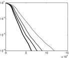
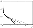
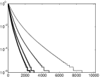
      a9a

cod-rna

      gisette scale

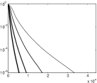
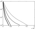
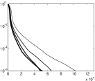
      real-sim

rcv1

         w8a

Figure 1: PARSMO-1: Relative Error versus iterations.

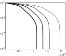
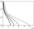
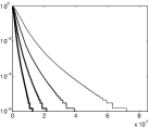
      a9a

cod-rna

      gisette scale

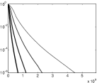
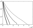
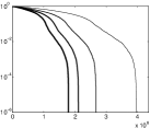
      real-sim

rcv1

         w8a

Figure 2: PARSMO-1: Relative Error versus kernel evaluations per process.

Our results show that the larger $q$ is, the steeper the $RE$ decrease is. This emphasizes the positive effect of moving along multiple SMO directions at a time.

As regards PARSMO-2, we note that, except for the MVP pair which can require the computation of the kernel columns ${Q}_{*i_{1}}$ and ${Q}_{*j_{1}}$, each SMO process computes only the analytical solution of the two-dimensional subproblem, since kernel columns are already available in the cache. Thus, PARSMO-2 may produce a cpu time saving even by running the algorithm in a sequential fashion. In order to show the cheapness of its tasks, in Figure 3 we plot $RE$ versus the CPU-time consumed.

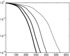
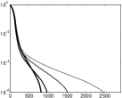
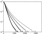
      a9a

cod-rna

      gisette scale

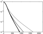
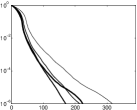
      real-sim

rcv1

         w8a

Figure 3: PARSMO-2: Relative Error versus (sequential) CPU-time.

PARSMO-2 with $q>1$ seems to be faster than a classical MVP algorithm. This is due the use of multiple search directions without suffering from an increase of time consuming kernel evaluations or from the need of iterative solutions of larger quadratic subproblems. It is important to outline that PARSMO-2 achieves its good performances by combining a convergent parallel structure with an efficient sequential implementation, and it seems to be useful also in a single-core environment.

References

• [1] D. P. Bertsekas. Nonlinear Programming. Athena Scientific, 1995.
• [2] L. J. Cao, S. S. Keerthi, C.-J. Ong, J. Q. Zhang, and H. P. Lee. Parallel sequential minimal optimization for the training of support vector machines. IEEE Trans. Neural Netw., 17(4):1039–1049, July 2006.
• [3] C.-C. Chang and C.-J. Lin. LIBSVM: A library for support vector machines. ACM Trans. Intell. Syst. Tech., 2:27:1–27:27, 2011.
• [4] P.-H. Chen, R.-E. Fan, and C.-J. Lin. A study on SMO-type decomposition methods for Support Vector Machines. IEEE Trans. Neural Netw., 17(4):893–908, 2006.
• [5] C. Cortes and V. Vapnik. Support-vector networks. Mach. Learn., 20(3):273–297, 1995.
• [6] A. Dreves, F. Facchinei, C. Kanzow, and S. Sagratella. On the solution of the KKT conditions of generalized Nash equilibrium problems. SIAM J. Optim., 21(3):1082–1108, 2011.
• [7] F. Facchinei and C. Kanzow. Generalized Nash equilibrium problems. 4OR, 5(3):173–210, 2007.
• [8] F. Facchinei and S. Sagratella. On the computation of all solutions of jointly convex generalized Nash equilibrium problems. Optim. Lett., 5(3):531–547, 2011.
• [9] F. Facchinei, G. Scutari, and S. Sagratella. Parallel selective algorithms for nonconvex big data optimization. IEEE Trans. Signal Process., 63(7):1874–1889, April 2015.
• [10] R.-E. Fan, K.-W. Chang, C.-J. Hsieh, X.-R. Wang, and C. J. Lin. LIBLINEAR: A library for large linear classification. J. Mach. Learn. Res., 9:1871–1874, 2008.
• [11] M. C. Ferris and T. S. Munson. Interior-point methods for massive support vector machines. SIAM J. Optim., 13(3):783–804, 2002.
• [12] H. P. Graf, E. Cosatto, L. Bottou, I. Dourdanovic, and V. Vapnik. Parallel support vector machines: The cascade SVM. In Advances in Neural Information Processing Systems, pages 521–528.
• [13] T. Joachims. Making large scale SVM learning practical. In C.B.B. Schölkopf, C.J.C. Burges, and A. Smola, editors, Advances in Kernel Methods - Support Vector Learning. MIT Press, Cambridge, MA, 1999.
• [14] S. S. Keerthi and E. G. Gilbert. Convergence of a generalized SMO algorithm for SVM classifier design. Mach. Learn., 46(1-3):351–360, 2002.
• [15] C.-J. Lin. On the convergence of the decomposition method for support vector machines. IEEE Trans. Neural Netw., 12:1288–1298, 2001.
• [16] C.-J. Lin. Asymptotic convergence of an SMO algorithm without any assumptions. IEEE Trans. Neural Netw., 13:248–250, 2002.
• [17] C.-J. Lin. A formal analysis of stopping criteria of decomposition methods for support vector machines. IEEE Trans. Neural Netw., 13(5):1045–1052, 2002.
• [18] G. Liuzzi, L. Palagi, and M. Piacentini. On the convergence of a jacobi-type algorithm for singly linearly-constrained problems subject to simple bounds. Optim. Lett., 5(2):347–362, 2011.
• [19] S. Lucidi, L. Palagi, A. Risi, and M. Sciandrone. A convergent hybrid decomposition algorithm model for SVM training. IEEE Trans. Neural Netw., 20(6):1055–1060, 2009.
• [20] L. Palagi and M. Sciandrone. On the convergence of a modified version of SVMlight algorithm. Optim. Methods Softw., 20(2-3):317–334, 2005.
• [21] J. C. Platt. Advances in kernel methods. chapter Fast Training of Support Vector Machines Using Sequential Minimal Optimization, pages 185–208. MIT Press, Cambridge, MA, USA, 1999.
• [22] A. Risi. Convergent decomposition methods for Support Vector Machines. PhD thesis, Sapienza University of Rome, 2008.
• [23] J. Shawe-Taylor and N. Cristianini. Kernel Methods for Pattern Analysis. Cambridge University Press, New York, NY, USA, 2004.
• [24] P. Tseng and S. Yun. A coordinate gradient descent method for linearly constrained smooth optimization and support vector machines training. Comput. Optim. Appl., 47(2):179–206, 2010.
• [25] J. Yang. An improved cascade SVM training algorithm with crossed feedbacks. In Computer and Computational Sciences, 2006. IMSCCS ’06. First International Multi-Symposiums on, volume 2, pages 735–738, June 2006.
• [26] G. Zanghirati and L. Zanni. A parallel solver for large quadratic programs in training support vector machines. Parallel Comput., 29(4):535 – 551, 2003.
• [27] L. Zanni, T. Serafini, and G. Zanghirati. Parallel software for training large scale support vector machines on multiprocessor systems. J. Mach. Learn. Res., 7:1467–1492, 2006.
• [28] J.-P. Zhang, Z.-W. Li, and J. Yang. A parallel SVM training algorithm on large-scale classification problems. In Machine Learning and Cybernetics, 2005. Proceedings of 2005 International Conference on, volume 3, pages 1637–1641 Vol. 3, Aug 2005.
• [29] G. Zoutendijk. Methods of Feasible Directions: a Study in Linear and Non-Linear Programming. Elsevier, 1960.