Abstract

We review some theories of non-equilibrium Bose-Einstein condensates in potentials, in particular of the Bose-Einstein condensate of polaritons. We discuss such condensates, which are steady-states established through a balance of gain and loss, in the complementary limits of a double-well potential and a random disorder potential. For equilibrium condensates, the former corresponds to a Josephson junction, whereas the latter is the setting for the superfluid/Bose glass transition. We explore the non-equilibrium generalization of these phenomena, and highlight connections with mode selection and synchronization.

Chapter 0 Disorder, synchronization and phase locking in non-equilibrium Bose-Einstein condensates

1 Introduction

It is twenty years since Bose-Einstein condensation (BEC) was achieved, in its ideal setting of a weakly-interacting ultracold gas. In other settings, namely superconductivity (which we understand in terms of a Bose-Einstein condensate of Cooper pairs), Bose-Einstein condensates have been available in laboratories for over a century. Yet their behaviour is still startling. Because the many particles of the condensate occupy the same quantum state, collective properties become described by a macroscopic wavefunction, with an interpretation parallel to that of the single-particle wavefunction of Schrödinger’s equation. Thus, many of the phenomena of single-particle quantum mechanics appear as behaviours of the condensate.

At the mean-field level a BEC is described by an order parameter $\Psi$, which is a complex field $\Psi(r,t)=\sqrt{n}e^{i\phi}$. Its square modulus is the local condensate or superfluid density, and it obeys the Schrödinger-like Gross-Pitaevskii equation. Because the order is described by a complex field, i.e., there is a spontaneous breaking of a U(1) symmetry, there is a new conserved current, given by the usual probability current of a wavefunction. This describes the condensate contribution to the macroscopic current flow in the fluid.

The wavelike behaviour of condensates leads to interesting effects in a potential. For the simple double-well potential, and related two-state problems, one obtains the Josephson effects [1]. In particular, the double-well junction system supports a d.c. Josephson state, with a current flowing corresponding to a difference in the phases $\phi$ of the two wells. Because the phase is compact there is a maximum current supported by such a state; attempting to impose a larger current by external bias typically leads to an a.c. Josephson state, where the relative phase oscillates or winds. The other extreme is a complex disorder potential, where it is natural to ask whether the ordered state survives, i.e., whether there some global phase established across the system, and hence whether the disordered system supports superfluidity [2]. This problem is closely related to wave localization, and the result is that superfluidity persists up to a critical disorder strength where the order is destroyed, leading to a glass-like state.

The aim of this chapter is to review some theories of how these phenomena generalize to non-equilibrium Bose-Einstein condensates. We have in mind, primarily, the Bose-Einstein condensate of polaritons. Here there is a continuous gain and loss of particles in the condensate, due to pumping and decay. However, the concepts are also relevant to other topical non-equilibrium condensates, including those of magnons and photons, and are linked to aspects of laser physics. Our aim is not a comprehensive review. Rather we hope to indicate a unifying framework for understanding non-equilibrium condensates in inhomogeneous settings, from Josephson-like double-well systems, to complex disorder potentials. We think that these problems can be understood in terms of the synchronization and phase-locking of coupled oscillators, as well as the related phenomenology of mode selection in lasers. The connection between synchronization and the physics of equilibrium Josephson junctions is well-known, and reviewed, for example, in Ref. [3].

2 Models of non-equilibrium condensation

As the basis for discussing non-equilibrium BEC we will use a generalization of the Gross-Pitaevskii equation (GPE) in the form [4]

$$i\hbar\partial_{t}\Psi\ =\ \left[-\frac{\hbar^{2}}{2m}+V(\mathbf{x})\right]\Psi+U|\Psi|^{2}\Psi+\ i(\gamma-\Gamma|\Psi|^{2})\Psi,$$ (1)

for definiteness supposing two space dimensions, as appropriate to microcavity polaritons. $\Psi(\mathbf{x},t)$ is the macroscopic wave-function for the condensate. The first three terms on the right-hand side comprise the usual GPE [1], with contributions from the kinetic energy, potential energy, and repulsive interactions. The terms in the final bracket model, in a phenomenological way, a continual gain and loss of particles in the condensate, due to scattering into and out of external incoherent reservoirs. Noting that $|\Psi|^{2}$ is the condensate density, we see that the term proportional to $i\gamma$ generates an exponential growth or decay of the condensate. In general it combines the effects of stimulated scattering into the condensate from a reservoir, and spontaneous emission out of it into another. If the former exceeds the latter $\gamma>0$ and the net effect is an exponential growth, so that $\gamma=0$ marks the threshold for condensation. Above threshold the condensate density builds up and the growth rate is reduced by the nonlinear term proportional to $\Gamma$, reaching zero at a steady-state density which, in the homogeneous case, is $n_{0}=\gamma/\Gamma$. In the language of laser physics this final term is the lowest-order nonlinear gain [5], describing the depletion of the gain by the build-up of the condensate. The scattering of particles into the condensate causes, in addition to its growth, a reduction of the occupation in the gain medium, and hence a reduction in the linear gain. The linear growth rate, $\gamma$, can of course vary with position, for example where the external pumping, and so the reservoir population, is inhomogeneous.

The generalized Gross-Pitaevskii model (1) was introduced for polariton Bose-Einstein condensation by Keeling and Berloff [4]. It is closely related to the GPE introduced by Wouters and Carusotto [6], in which the gain depends explicitly on a reservoir population, which in turn obeys a related first-order rate equation. Such a theory reduces to (1) if the reservoir population can be adiabatically eliminated, and the gain expanded in powers of the condensate density. Whether this is correct will depend on the scattering rates in the reservoir and hence the relaxation time for its population.

There are many other interesting extensions of the model (1) that may be considered. In particular, it is a mean-field equation that ignores the stochastic nature of the gain and loss process. In reality these lead to fluctuations in the condensate density, which have an observable signature in the finite linewidth of the light emitted from the polariton condensate [7] (i.e., a finite correlation time for the U(1) phase). Both single-mode and multi-mode theories including such fluctuations have been developed within the density matrix formalism [8]. They can be treated within the GPE by introducing stochastic terms, related by the fluctuation-dissipation theorem to the gain and loss [9, 10]. Such stochastic GPEs have been derived from the truncated Wigner approximation [9], and used to study the coherence properties of polariton condensates. Another, potentially important extension, is to allow some degree of thermalization with the reservoirs, which corresponds to a frequency-dependent gain.

In the following we shall focus on two specific applications of (1). Firstly, we consider a double-well with a single relevant orbital on each side. In the usual way [11] we may expand the wavefunction in terms of the amplitudes for the left and right wells as $\Psi(\mathbf{x},t)=\Psi_{l}(t)\phi_{l}(\mathbf{x})+\Psi_{r}(t)\phi_{r}(\mathbf{x})$, where $\phi_{l,r}$ are wavefunctions localized on the left and right. Inserting this into (1) gives the equations for the amplitudes $\Psi_{l,r}$:

$$i\hbar\frac{d\Psi_{l}}{dt} =\frac{\epsilon}{2}\Psi_{l}-J\Psi_{r}+U_{l}|\Psi_{l}|^{2}\Psi_{l}+i[g_{l}-\Gamma_{l}|\Psi_{l}|^{2}]\Psi_{l},$$

$$i\hbar\frac{d\Psi_{r}}{dt} =-\frac{\epsilon}{2}\Psi_{r}-J\Psi_{l}+U_{r}|\Psi_{r}|^{2}\Psi_{r}+i[g_{r}-\Gamma_{r}|\Psi_{l}|^{2}]\Psi_{r},$$ (2)

assuming the overlap of $\phi_{l}$ and $\phi_{r}$ is small. Here $\epsilon$ is the energy difference between the wells, and $J$ is the tunnelling matrix element. $g_{l,r}$ corresponds to the gain/loss of each well, $g_{l,r}=\int\phi_{l,r}^{\ast}\gamma\phi_{l,r}\,d^{2}\mathbf{x}$. If the pumping is uniform $\gamma$ is independent of position and $g_{l}=g_{r}=\gamma$. $U_{l,r}$ and $\Gamma_{l,r}$ are the nonlinearities for each well, $\Gamma_{l,r}=\int|\phi_{l,r|}|^{4}\Gamma\,d^{2}\mathbf{x}$. Secondly, we shall consider a non-equilibrium condensate in a random disorder potential. Thus we will consider Eq. (1) with $V$ being a Gaussian random potential, whose correlation function is characterized by its first two moments, which we take to be $\langle\langle V(\mathbf{x})\rangle\rangle=0$ and $\langle\langle V(\mathbf{x})V(\mathbf{y})\rangle\rangle=V_{0}^{2}\delta^{(2)}(\mathbf{x}-\mathbf{y})$, where angle brackets denote an average over disorder realizations.

3 Josephson effects and synchronization

The physics of synchronization and phase-locking is well described elsewhere, for example in Ref. [3], so we summarize it only briefly. The starting point is the idea that self-sustained oscillators, which oscillate at their own frequencies when isolated, can be coupled together. We will say that oscillators are synchronized if they oscillate at a common frequency. Synchronization is the phenomenon that oscillators become synchronized when coupled. This occurs above a critical coupling which increases with the detuning, i.e., the difference in frequencies when uncoupled. Two oscillators with the same intrinsic frequency are of course synchronized, in our sense, even for zero coupling, but for detuned oscillators a non-zero coupling is required if they are to establish a common frequency. We will also use the term phase-locked, by which we mean that the coupling establishes some definite relation between the phases of the oscillations. This is stronger than our notion of synchronized. Note that the definitions of these terms are not standardised, and some other authors use them somewhat differently.

The relevance of this physics to the non-equilibrium Josephson junction, Eq. (2), is immediate. When the tunnelling $J=0$ the equations decouple. Each well is a self-sustained oscillator with its own frequency. The steady-state amplitude of the left well, for example, is $\Psi_{l}=\sqrt{n_{0,l}}e^{-i\omega_{l}t+i\theta_{l}}$, with occupation $n_{0,l}=g_{l}/\Gamma_{l}$. $\omega_{l}=(\epsilon/2+U_{l}n_{0,l})/\hbar$ is the frequency of this oscillator, with a corresponding expression, with $\epsilon\rightarrow-\epsilon$, $l\rightarrow r$, for the other. $\theta_{l}$ and $\theta_{r}$ are arbitrary, and independent, phase offsets.

The Josephson coupling term, proportional to $J$, allows these oscillators to drive one another. Because the oscillators are nonlinear, as described by the terms proportional to both $U$ and $\Gamma$, their phases become coupled. A physical picture of this is that as the oscillators force one another their amplitudes change, which changes their frequency difference through the nonlinearity, and hence shifts their relative phase. This can establish a steady-state with a constant relative phase and a single frequency.

As a simple model of synchronization one might suggest that a suitably defined relative phase $\delta$ should obey an equation of the form [3]

$$\frac{d\delta}{dt}=-(\omega_{l}-\omega_{r})+c\sin(\delta),$$ (3)

on the grounds that the first term generates the appropriate winding when the oscillators are uncoupled, and the second is the simplest coupling one can write consistent with the $2\pi$ periodicity. This is the Adler equation, which can be seen to have solutions of both constant relative phase, and continuously increasing relative phase. The case of a constant relative phase corresponds to a steady-state solution to Eqs. (2) of the form

$$\Psi_{l,r}=\sqrt{n_{l,r}}e^{-i\omega t\pm i\theta/2}e^{i\theta_{0}},$$ (4)

which contains a single frequency $\omega$, and a single undetermined phase $\theta_{0}$.

The conditions for a synchronized solution for the dissipative double-well can be established by inserting Eq. (4) into Eq. (2), and examining whether there are physical solutions to the resulting equations. This approach was taken by Wouters [12], using a slightly more complex model. In particular, he obtains the conditions on the detuning and tunnelling required for the synchronized solution, and the predicts properties of the states. The dynamics of the two-mode problem is also treated in this way in Ref. [13], where the two modes correspond to two polarizations. A recent numerical analysis of that problem can be found in Ref. [10].

We summarize this type of steady-state analysis of the two-mode model using Eq. (2). For simplicity we take the two wells to be identical, so that $g_{l}=g_{r}=g$, etc.. It is convenient to choose $n_{0}=g/\Gamma$ to be the density scale, by replacing $\Psi_{l}\to\Psi_{l}\sqrt{n_{0}}$, so that $n_{l,r}=1$ in the uncoupled steady-state. We also set $\hbar=1$ and take as the energy scale $Un_{0}$. From (2) and (4) we then find

$$\alpha(1-n_{l})n_{l}=-J\sqrt{n_{l}n_{r}}\sin(\theta)=-\alpha(1-n_{r})n_{r},$$ (5)

$$E_{l}n_{l}=J\sqrt{n_{l}n_{r}}\cos(\theta)=E_{r}n_{r},$$ (6)

where $\alpha,J,E_{l}$ and $E_{r}$ are energies measured in units of $Un_{0}$. $\alpha=g/(Un_{0})=\Gamma/U$ is a dimensionless measure of the gain, and $E_{l,r}=\pm\frac{\epsilon}{2}-\omega+n_{l,r}$ the energies of each well, including the mean-field shifts, relative to $\omega$. Note that $\alpha\rightarrow 0$ corresponds to the unpumped Josephson junction, whereas $\alpha\rightarrow\infty$ is the limit where the interaction $U$ is negligible as, for example, in a laser.

Eq. (5) describes current flows in the non-equilibrium double-well. The term on the far left corresponds to the net current flowing between the reservoirs and the left well. If the density there deviates from $n_{l}=1$ the gain will no longer be reduced to zero by the nonlinear term, and there will be a source ($n_{l}<1$) or sink ($n_{l}>1$) of particles. In a steady-state this current must flow into the other well, as the Josephson current visible in the centre of the chain of equalities. It must then match the current flowing between the right well and the reservoirs, which is the quantity on the right. Eq. (6) is a related condition, stating that the two wells must be in mechanical equilibrium through the Josephson coupling.

The presence of trigonometric functions in Eqs. (5) and (6), which have magnitude less than one, is why the synchronized solution only exists over limited parameter regimes. In particular, Eq. (5) limits the range of $J$ in which there is a synchronized solution, and Eq. (6) limits the range of detunings $\epsilon$. Consider, for example, starting in a synchronized solution with $\epsilon=0$. Then as $\epsilon$ increases the real part of the steady-state equation, which is essentially Schrödinger’s equation for a double-well, will concentrate the wavefunction to one side or another. For such a wavefunction the pumping will generate a net interwell current. If this exceeds the Josephson critical current $J\sqrt{n_{l}n_{r}}$ then the synchronized steady-state breaks down. The transition is thus analogous to that between the d.c. and a.c. Josephson effects, but with currents generated by gain and loss, rather than external bias.

A complementary route to understanding the physics of non-equilibrium condensates in potentials, and particularly the presence of both synchronized and desynchronized states, is to relate it to that of mode selection in lasers. For polariton condensates this was done by one of us [14] using the model of Eq. (1). We outline it here for comparison.

The general approach is to take those parts of Eqs. (1) or  (2) that form the Schrödinger equation as an unperturbed problem. The remainder can then be dealt with using a form of degenerate perturbation theory. To do this we expand the solutions in terms of the orbitals which are eigenfunctions of the first bracket in Eq. (1). We assume two states, for simplicity, and write $\Psi(\mathbf{x},t)=\Psi_{1}(t)\phi_{1}(\mathbf{x})+\Psi_{2}(t)\phi_{2}(\mathbf{x})$ . The time-dependence of the unperturbed amplitudes will be $\Psi_{1,2}(t)=e^{-iE_{1,2}t/\hbar}$, where $E_{1,2}$ are the energies of $\phi_{1,2}$. For Eqs. (2) the Schrödinger part is explicitly diagonalized by a rotation, writing $\Psi_{l,r}=\cos(\theta)\Psi_{1}\mp\sin(\theta)\Psi_{2}$ and choosing $\tan(2\theta)=-2J/\epsilon$.

Such a unitary transformation leaves the equations-of-motion for the amplitudes $\Psi_{1}$ and $\Psi_{2}$ coupled, because it neither diagonalizes the interactions, nor the linear gain terms (unless $g_{l}=g_{r}$). However, these off-diagonal terms can be neglected if their magnitudes are small compared with the unperturbed level spacing $E_{1}-E_{2}$. For the nonlinear couplings, this requires that the nonlinearities (both the mean-field shift $Un_{0}$ and the corresponding scale from the gain depletion, $\Gamma n_{0}$) are small compared with the level spacing.

In the equations-of-motion the off-diagonal couplings correspond to terms which oscillate at frequencies of order $E_{1}-E_{2}$ and therefore average to zero. In the energy functional, they are terms such as $\Psi_{1}^{\ast}\Psi_{1}^{\ast}\Psi_{2}\Psi_{2}$ (from the interactions) and $\Psi_{1}^{\ast}\Psi_{2}$ (from the linear gain) which, in a quantized theory, describe scattering processes that do not conserve energy. Retaining only the resonant terms gives

$$i\hbar\frac{d\Psi_{1,2}}{dt}=[E_{1,2}+ig_{1,2}+(U-i\Gamma)(\eta_{1,2}|\Psi_{1,2}|^{2}+2\beta|\Psi_{2,1}|^{2})]\Psi_{1,2},$$ (7)

were we suppose only two states, and nonlinearities which do not depend on position, for simplicity. Here $g_{1,2}$ are diagonal matrix elements of the linear gain for orbitals $\phi_{1},\phi_{2}$, cf., the discussion after Eq. (2). $\eta_{1,2}=\int|\phi_{1,2}|^{4}d^{2}\mathbf{x}$ and $\beta=\int|\phi_{1}|^{2}|\phi_{2}|^{2}d^{2}\mathbf{x}$ are matrix elements of the nonlinearities within and between the single-particle orbitals, respectively. It follows from Eq. (7) that the occupations obey

$$\hbar\partial_{t}n_{1,2}=2[g_{1,2}-\Gamma(\eta_{1,2}n_{1,2}+\beta n_{2,1})]n_{1,2}.$$ (8)

Equations like (8) describe mode competition in lasers with local gain [5]. The linear term gives an exponential growth of each mode, which is controlled by gain depletion effects. The build up of one mode of course reduces its own gain, as described by the term proportional to $\eta$, but it also reduces the gain for any other mode which shares the same gain medium, i.e., overlaps in space. This cross-gain-depletion is the term proportional to $\beta$.

The steady-state structure of Eq. (8) is straightforward to determine, and reflects the density profiles of the orbitals [14]. For the general two-mode case there are states in which only one of $n_{1},n_{2}$ is non-zero. These are synchronized states, as they have only a single oscillation frequency, which corresponds to the energy of the occupied orbital, shifted by interactions. Note that although the orbitals involved are linear eigenstates, the synchronization itself is due to nonlinearities: it is the nonlinear gain which selects an eigenstate in which to form the condensate. Furthermore, there are also states in which $n_{1}\neq 0,n_{2}\neq 0$. These are the desynchronized states, with oscillations at two frequencies, analogous to the a.c. Josephson state.

We conclude this discussion by commenting on a few of the many experiments addressing these issues with microcavity polaritons. For polaritons the difference between synchronized and desynchronized states of polaritons is immediate, because $\Psi$ is the amplitude of the macroscopic component of the electric field in the microcavity. The spectrum of $\Psi$ thus corresponds to the spectrum of the light emitted from the microcavity. Thus in a potential with two relevant orbitals the synchronized state has one single narrow emission line, and the desynchronized state two. In the language of laser physics, it is a distinction between single- and multi-mode lasing.

The double-well was studied experimentally in Ref. [15], and oscillations in the intensity observed in the time domain. Such oscillations would be expected where two linear eigenmodes of a double well are both highly occupied, i.e., in a multi-mode condensate. The experiment, however, is not completely consistent with that picture. The density oscillations have a deterministic phase, implying that there are processes which fix the relative phase of the two macroscopically-occupied orbitals. These can be found among the terms neglected above. Simulations including them can be found alongside the experiments, and show good agreement.

Particularly in extended geometries, where there is a potential due to in-plane disorder, polariton condensates do emit at many distinct frequencies [16]. A detailed study of the spectra was performed by Baas et al. [17], who identified pairs of modes which, while having independent frequencies at low densities, locked to a single frequency above a critical density. The low density state thus appears consistent with Eq. (7). The transition to a synchronized states occurs due to the neglected nonlinear coupling terms. In particular, increasing density in a multi-mode solution leads first to nonlinear mixing effects, which finally drive the formation of a synchronized state. This is shown numerically in Ref. [14].

4 The Bose glass and phase locking

We know turn to consider the complementary problem of a non-equilibrium condensate in a random potential, reviewing first the interplay of disorder and BEC in two dimensions, as discussed in [2]. Due to the localization effects of randomness, one expects that sufficiently strong disorder causes a destruction of superfluidity. The resulting phase is called a Bose glass, and is characterized by a finite compressibility $\kappa={\partial n/\partial\mu}$, has gapless excitations with a finite density of states at zero energy, and as a consequence has infinite superfluid susceptibility. The susceptibility is determined by the ensemble averaged retarded correlation function

$$G^{R}({\mathbf{x}},t)=-i\theta(t)\langle\langle[\Psi({\mathbf{x}},t),\Psi^{\dagger}(0,0)]\rangle\rangle\ \ ,$$ (9)

where $[,]$ denotes the commutator, $\langle\langle{\cdots}\rangle\rangle$ the combined average over disorder and quantum fluctuations, and $\theta(t)$ the Heaviside step function. Due to the localizing effects of disorder, $G^{R}$ decays exponentially as a function of distance. The local Green function can be represented in terms of the single particle density of states $\rho(\omega)$ as

$$G^{R}(0,t)\ =\ 2\pi i\theta(t)\int_{0}^{\infty}d\omega\rho(\omega)\,e^{-i\omega t}\ \ .$$ (10)

Here, the quasi-particle energy is measured with respect to the chemical potential. When there is a finite density of states at zero energy, $\rho(0)\neq 0$, then the long time asymptotics of the Green function is given by $G^{R}(t)\sim 2\pi\rho(0)\theta(t)/t$, giving rise to a divergent uniform superfluid susceptibility $\xi=\int d^{d}rdtG^{R}({\mathbf{r}},t)$. The susceptibility is dominated by rare localized regions which have anomalously low quasiparticle excitation energies. While much of the focus in [2] is on the scaling behaviour of the superfluid Bose glass and also the superfluid insulator transition, the competition between a disorder potential and its screening by a weak repulsive interaction in the presence of a harmonic trap was discussed in [18].

An analysis of the superfluid to Bose-glass transition with a focus on polariton condensates was presented in [19]. There, the excitation spectrum of the system was be obtained by computing stationary solutions the GPE, $\Psi_{j}({\mathbf{r}},t)=\Psi_{j}({\mathbf{r}})\exp(-i\omega_{j}t)$. From these solutions, the retarded Green function can be obtained as

$$G^{R}({\mathbf{x}},{\mathbf{x}}^{\prime};\omega)\ =\ \sum_{j}{\Psi_{j}({\mathbf{x}})\Psi^{\star}_{j}({\mathbf{x}}^{\prime})\over\omega-\omega_{j}+i\eta}.$$ (11)

Fourier transformation with regards to ${\mathbf{r}}-{\mathbf{r}}^{\prime}$ allows to obtain an excitation spectrum comparable to experimental observations [19]. For a chemical potential below the bottom of the disordered parabolic band, the system is almost empty, there are no excitations at the chemical potential, and the superfluid susceptibility does not diverge. Introducing a finite density of bosons, first the potential minima (traps) with the lowest energy are filled. Due to the density dependent blue shift, the density in each trap adjusts itself in such a way that it is filled up to the chemical potential, and there are many low energy excitations, giving rise to a diverging superfluid susceptibility as discussed above. The compressibility of this Bose glass state is finite since in the absence of a periodic potential there are many states available to be filled. Increasing the density further, the local condensates increase in size, until the different condensate puddles connect with each other to a percolating cluster, which then represents a global superfluid. The order parameter for this transition is the superfluid density or superfluid fraction as discussed below in Eq. (17). In [19], the superfluid fraction is computed numerically as a function of the condensate density, and good agreement is found with static analytical calculation discussed below.

Insight about the destruction of superfluidity by disorder can be gained from an Imry-Ma type argument for pinning by weak disorder [20, 21, 18] of a fragmented condensate cloud of radius $R$. Localizing the condensate within a spatial region of radius $R$ costs kinetic energy, but allows the condensate to lower its potential energy by taking advantage of local minima of the disorder potential, giving rise to a total energy

$$\epsilon(R)\ =\ {\hbar^{2}\over 2m}{1\over R^{2}}\ -\ {V_{0}\over\sqrt{\pi}R}\ \ .$$ (12)

The disorder energy decreases inversely proportional to the square root of the cloud area due to averaging over independent local fluctuations of the random potential. Minimizing this energy yields the density Larkin length $\mathcal{L}_{\mathrm{n}}=\sqrt{\pi}\hbar^{2}/mV_{0}$. Superfluidity is destroyed when the density Larkin length is equal to the healing length $\xi=\sqrt{\hbar^{2}/2mn_{0}U}$, giving rise to a critical density for the onset of superfluidity $n_{c}=mV_{0}^{2}/2\pi\hbar^{2}U$.

In the following, we provide a more quantitative discussion of the Bose glass superfluid transition, and include the influence of non-equilibrium. We analyze the dimensionless form of Eq. (1),

$$i\partial_{t}\Psi\ =\ (-\nabla^{2}+\vartheta+|\Psi|^{2})\Psi\ +\ i\alpha(1-|\Psi|^{2})\Psi\ \ ,$$ (13)

where we measure length in units of the healing length $\xi$, energy in units of the blueshift $n_{0}U$, and time in units of $\hbar/n_{0}U$. The strength of non-equilibrium fluctuations is controlled by the parameter $\alpha=\Gamma/U$. We assume that the correlation length of the disorder potential is the shortest length scale in the problem, such that the Gaussian random potential can be characterized by its average values $\langle\langle\vartheta({\mathbf{x}})=0\rangle\rangle$ and $\langle\langle\vartheta({\mathbf{x}})\vartheta({\mathbf{y}})\rangle\rangle=\kappa^{2}\delta({\mathbf{x}}-{\mathbf{y}})$. The dimensionless disorder strength is related to the dimensionful parameters via $\kappa=V_{0}/\xi^{d/2}n_{0}U$.

In the synchronized regime, the polariton condensate emits coherent light at a frequency $\omega$, which can be described by the ansatz

$$\Psi({\mathbf{x}},t)\ =\ \sqrt{n({\mathbf{x}})}\,e^{i\phi({\mathbf{x}})-i\omega t}\ \ .$$ (14)

Following the discussion in [22], the condensate frequency $\omega$ can be computed by inserting this ansatz into Eq. (13). The real part gives

$$\omega=(\nabla\phi)^{2}-{1\over 4}{(\nabla n)^{2}\over n^{2}}-{1\over 2}{\nabla^{2}n\over n}+n-\vartheta\ \ ,$$ (15)

which is a pressure balance equation analogous to Eq. (6). The imaginary part gives the analog of Eq. (5),

$$\nabla\cdot(n\nabla\phi)\ =\ \alpha n(1-n)\ \ ,$$ (16)

which is a continuity equation for the supercurrent, including the sources and sinks generated, via the gain depletion, by density fluctuations.

In the absence of disorder, the Bogolubov excitation mode is diffusive out of equilibrium [6], and a naive application of the Landau stability criterion yields a vanishing superfluid velocity. However, taking into account the imaginary part of the excitation energies, the drag force on a small moving object and the onset of fringes in the density profile are found to have a sharp threshold as a function of the velocity [23]. Similarly, superfluidity is found to survive [24] if the superfluid density is defined via the irrotational response at long wavelengths. To establish the behaviour in the presence of disorder, we calculate the superfluid stiffness, which characterizes the superfluid Bose-glass transition. To do this we apply twisted boundary conditions $\phi_{\theta}({\mathbf{x}}+L{\mathbf{e}}_{\theta})-\phi_{\theta}({\mathbf{x}})=\theta$. For the actual calculation, we apply a local transformation $\nabla\phi_{\theta}=\nabla\phi+\mathbf{A}_{\theta}$ with a twist current $\mathbf{A}_{\theta}=(\theta/L)\mathbf{e}_{\theta}$ with periodic boundary conditions imposed on $\phi({\mathbf{x}})$. The superfluid stiffness [25, 26] is then obtained from the frequency shift as

$$f_{s}\ =\ \lim_{\theta\to 0}{L^{2}\over\theta^{2}}[\omega(\theta)-\omega(0)]\ \ .$$ (17)

In the presence of weak disorder, we expand both the density and the condensate phase in powers of the disorder strength $\kappa$: $n=1+\eta_{(1)}+\mathcal{O}({\kappa^{2}})$ and $\nabla\phi=\nabla\phi_{(1)}+\mathcal{O}({\kappa^{2}})$ with $\eta_{(1)},\nabla\phi_{(1)}\sim\mathcal{O}({\kappa})$. From Eq. (15) we then obtain the expansion of the frequency shift. As the frequency shift is self-averaging, only even powers in $\kappa$ contribute. Odd powers of $\kappa$ in Eqs. (15,16) are used to compute the solutions for density and condensate phase according to $\eta_{1}({\mathbf{k}})=G_{\eta}({\mathbf{k}},{\mathbf{A}}_{\theta})\vartheta_{\mathbf{k}}$, $\phi_{1}({\mathbf{k}})=G_{\phi}({\mathbf{k}},{\mathbf{A}}_{\theta})\vartheta_{\mathbf{k}}$ with the Green functions [22]

$$G_{\eta}(\mathbf{k},{\mathbf{A}}_{\theta})=\frac{-k^{2}\chi_{k}}{k^{2}+2\>\mathrm{i}\mathbf{k}\cdot{\mathbf{A}}_{\theta}(\mathrm{i}\mathbf{k}\cdot{\mathbf{A}}_{\theta}+\alpha)\chi_{k}}\ ,$$ (18)

$$G_{\phi}(\mathbf{k},{\mathbf{A}}_{\theta})=\frac{-(\mathrm{i}\mathbf{k}\cdot{\mathbf{A}}_{\theta}+\alpha)\chi_{k}}{k^{2}+2\>\mathrm{i}\mathbf{k}\cdot{\mathbf{A}}_{\theta}(\mathrm{i}\mathbf{k}\cdot{\mathbf{A}}_{\theta}+\alpha)\chi_{k}},$$ (19)

with $\chi_{k}=(k^{2}/2+1)^{-1}$. These Green functions give the correlation functions of density and phase fluctuations in the ground state with ${\mathbf{A}}_{\theta}=0$. The correlation function for density fluctuations decays exponentially on the scale of the healing length, allowing density fluctuations to screen the disorder potential on short length scales. As discussed above, a weak disorder potential becomes important only on the scale of the density Larkin length $\mathcal{L}_{\mathrm{n}}\sim 1/\kappa$. The driven nature of the polariton condensate becomes apparent when considering phase fluctuations, which are imprinted onto the condensate by random sources and sinks as described by Eq. (16). Long range order is destroyed by these phase fluctuations on the scale of the phase Larkin length $\mathcal{L}_{\mathrm{\phi}}\sim 1/\alpha\kappa$, which is also the decay length of the phase correlation function.

In the next step we calculate the condensate stiffness using Eq. (17), perturbatively to order $\kappa^{2}$, finding

$$f_{s}\approx 1-\left\{c_{1}+g_{1}(L)\>\alpha^{2}+\left(g_{2}(L)+c_{2}L^{2}\right)\alpha^{4}\right\}\kappa^{2}\ ,$$ (20)

where we have omitted finite-size corrections vanishing for $L\to\infty$. The coefficients in this expansion are [22]

$$c_{1} =\frac{1}{2\pi}\ ,\qquad c_{2}=\frac{1}{(2\pi)^{3}}\ ,$$

$$g_{1}(L) =-\frac{1}{\pi}\left(\log\frac{2L^{2}}{(2\pi)^{2}}-\frac{19}{12}\right),$$

$$g_{2}(L) =-\frac{1}{\pi}\left(\log\frac{2L^{2}}{(2\pi)^{2}}-\frac{13}{12}\right).$$

In the equilibrium limit, $\alpha\to 0$, this reproduces previous findings  [27, 28, 29]: the stiffness is zero above a critical $\kappa=\sqrt{2\pi}$. For finite $\alpha$, however, the stiffness is driven to zero for any $\kappa\neq 0$ beyond the length scale $\mathcal{L}_{\mathrm{s}}\sim 1/\alpha^{2}\kappa$. This indicates that for a driven system superfluidity is always destroyed in the thermodynamic limit.

One expects, from this perturbative result, that the stiffness reduction will scale with the parameter $\alpha^{4}\kappa^{2}L^{2}$. This is confirmed numerically [22], as shown in Fig. 1.

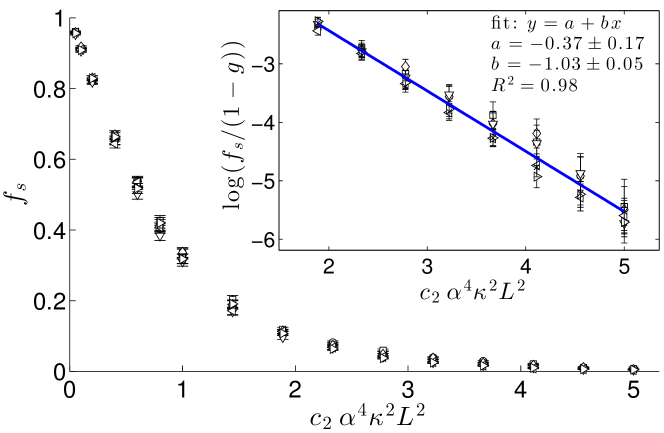
Figure 1: Test of the scaling form for the stiffness of a non-equilibrium condensate, Eq. (21). A clear data collapse is observed when plotting the numerically obtained superfluid stiffness as a function of $c_{2}\alpha^{4}\kappa^{2}L^{2}\sim L^{2}/{\mathcal{L}_{\mathrm{s}}}^{2}$. Inset: exponentially small tail of $f_{s}$ compared to the scaling form Eq. (21), using the perturbative values $c_{2}$ and $g$. Data points for $L\times L$ lattices with $L=64$ and $96$; $\alpha=0.9,1$ and $1.2$, and for up to $1320$ disorder realizations. Figure taken from [22].

The numerically computed stiffness decays exponentially for large values of the parameter $c_{2}\alpha^{4}\kappa^{2}L^{2}\sim L^{2}/{\mathcal{L}_{\mathrm{s}}}^{2}$. Using this insight, we propose a scaling form for the superfluid stiffness which reproduces both the perturbative results for small values of the scaling parameter, and which displays an exponential decay for large values

$$f_{s}=e^{-c_{2}\,\alpha^{4}\kappa^{2}L^{2}}(1-g(\alpha,\kappa,\log L))\ \ .$$ (21)

In Fig. 1, the numerically computed stiffness is plotted as a function of the scaling variable $c_{2}\alpha^{4}\kappa^{2}L^{2}\sim L^{2}/{\mathcal{L}_{\mathrm{s}}}^{2}$ to demonstrate data collapse, confirming the validity of scaling and the specific form of the scaling function above.

What is the interpretation of the length scale $\mathcal{L}_{\mathrm{s}}\propto 1/\alpha^{2}\kappa$ for the decay of superfluidity? Imposing twisted boundary conditions and following the difference $\nabla\phi_{\theta}-\nabla\phi$ for individual disorder realizations, one observes that the phase twist does not relax in a uniform manner from one boundary of the sample to the other, but rather relaxes over domain walls of width $\mathcal{L}_{\mathrm{s}}$. Since the relaxation of the phase twist $\theta$ imposes the existence of a local supercurrent $j=n(\nabla\phi_{\theta})$, it is energetically favourable for the relaxation to occur in spatial regions where the local distribution of current sources and sinks leads to a pinning of such a domain wall.

5 Summary

We have outlined how, within a generalized Gross-Pitaevskii model, gain and loss impact on the physics of condensates in potentials. For the double-well there is a transition between a synchronized and desynchronized state. These states can be understood in a similar way to the d.c. and a.c. Josephson effects, with the transition caused by currents associated with gain and loss, rather than external bias. A complementary perspective is that of mode selection in lasers, where the form of the nonlinear gain can select single or multi-mode behaviour. The key phenomena of Josephson oscillations and multi-mode polariton condensation have been observed experimentally. More recent experiments are further expanding the phenomenology of non-equilibrium condensation in few-mode systems.

Interest in the behaviour of Bose Einstein condensates in a disordered environment has been reinvigorated by experiments on Anderson localization of cold atomic gases. Polariton condensates naturally allow the observation of such physics, enriched by their non-equilibrium nature. Theory predicts it has a dramatic effect. The presence of condensate currents in the steady-state converts potential disorder to symmetry-breaking disorder [22, 30], which can destroy long-range order. Moreover, the absence of a true continuity equation allows a localized response to an imposed long-wavelength phase twist, so that the superfluid stiffness is driven to zero. The resulting disordered phase has a vanishing stiffness, like the Bose glass, and appears as soon as one departs from the equilibrium limit. This allows for the observation of phase-coherent phenomena and superfluidity as finite size effects only.

It would be interesting to attempt to observe this physics experimentally, as there are several open issues. One is whether the disordered phase really only has short-range order as predicted by perturbation theory, or whether this result is modified by non-perturbative effects. More broadly, it remains to establish the full phase diagram of the non-equilibrium problem, in terms of the parameters $\kappa$ and $\alpha$. At present we know there is an ordered phase for $\alpha=0,\kappa<\kappa_{c}$, and a disordered one for $\alpha\neq 0,\kappa\neq 0$. The disordered phase we describe above is, in the terminology of Sec. 3, synchronized (it has a single frequency) but not phase-locked (it has no stiffness). Experimentally and numerically, however, there is also a disordered phase which is neither synchronized nor phase-locked. This corresponds to the a.c. Josephson state of the double-well, or more generally to multi-mode condensation. It remains to determine whether this is a distinct disordered phase, and if so, where in parameter space it occurs.

References

- Leggett, [2001] Leggett, A. J. 2001. Bose-Einstein condensation in the alkali gases: some fundamental concepts. Rev. Mod. Phys., 73, 307–356.
- Fisher et al., [1989] Fisher, M. P. A., Weichman, P. B., Grinstein, G., and Fisher, D. S. 1989. Boson localization and the superfluid-insulator transition. Phys. Rev. B, 40, 546–570.
- Pikovsky et al., [2001] Pikovsky, A., Rosenblum, M., and Kurths, J. 2001. Synchronization. Cambridge, UK: Cambridge University Press.
- Keeling and Berloff, [2008] Keeling, J., and Berloff, N. G. 2008. Spontaneous rotating vortex lattices in a pumped decaying condensate. Phys. Rev. Lett., 100, 250401.
- Siegman, [1986] Siegman, A. E. 1986. Lasers. Oxford UK: Oxford University Press.
- Wouters and Carusotto, [2007] Wouters, M., and Carusotto, I. 2007. Excitations in a nonequilibrium Bose-Einstein condensate of exciton polaritons. Phys. Rev. Lett., 99, 140402.
- Love et al., [2008] Love, A. P. D., Krizhanovskii, D. N., Whittaker, D. M., Bouchekioua, R., Sanvitto, D., Rizeiqi, S. Al, Bradley, R., Skolnick, M. S., Eastham, P. R., André, R., and Dang, Le Si. 2008. Intrinsic decoherence mechanisms in the microcavity polariton condensate. Phys. Rev. Lett., 101, 067404.
- Racine and Eastham, [2014] Racine, D., and Eastham, P. R. 2014. Quantum theory of multimode polariton condensation. Phys. Rev. B, 90, 085308.
- Wouters and Savona, [2009] Wouters, M., and Savona, V. 2009. Stochastic classical field model for polariton condensates. Phys. Rev. B, 79, 165302.
- Read et al., [2010] Read, D., Rubo, Y. G., and Kavokin, A. V. 2010. Josephson coupling of Bose-Einstein condensates of exciton-polaritons in semiconductor microcavities. Phys. Rev. B, 81, 235315.
- Zapata et al., [1998] Zapata, I., Sols, F., and Leggett, A. J. 1998. Josephson effect between trapped Bose-Einstein condensates. Phys. Rev. A, 57, R28–R31.
- Wouters, [2008] Wouters, M. 2008. Synchronized and desynchronized phases of coupled nonequilibrium exciton-polariton condensates. Phys. Rev. B, 77, 121302(R).
- Borgh et al., [2010] Borgh, M. O., Keeling, J., and Berloff, N. G. 2010. Spatial pattern formation and polarization dynamics of a nonequilibrium spinor polariton condensate. Phys. Rev. B, 81, 235302.
- Eastham, [2008] Eastham, P. R. 2008. Mode locking and mode competition in a nonequilibrium solid-state condensate. Phys. Rev. B, 78, 035319.
- Lagoudakis et al., [2010] Lagoudakis, K. G., Pietka, B., Wouters, M., André, R., and Deveaud-Plédran, B. 2010. Coherent oscillations in an exciton-polariton Josephson junction. Phys. Rev. Lett., 105, 120403.
- Krizhanovskii et al., [2009] Krizhanovskii, D. N., Lagoudakis, K. G., Wouters, M., Pietka, B., Bradley, R. A., Guda, K., Whittaker, D. M., Skolnick, M. S., Deveaud-Plédran, B., Richard, M, André, R, and Dang, Le Si. 2009. Coexisting nonequilibrium condensates with long-range spatial coherence in semiconductor microcavities. Phys. Rev. B, 80, 045317.
- Baas et al., [2008] Baas, A., Lagoudakis, K. G., Richard, M., André, R., Dang, Le Si, and Deveaud-Plédran, B. 2008. Synchronized and desynchronized phases of exciton-polariton condensates in the presence of disorder. Phys. Rev. Lett., 100, 170401.
- Nattermann and Pokrovsky, [2008] Nattermann, T., and Pokrovsky, V. L. 2008. Bose-Einstein condensates in strongly disordered traps. Phys. Rev. Lett., 100, 060402.
- Malpuech et al., [2007] Malpuech, G., Solnyshkov, D. D., Ouerdane, H., Glazov, M. M., and Shelykh, I. 2007. Bose glass and superfluid phases of cavity polaritons. Phys. Rev. Lett., 98, 206402.
- Larkin, [1970] Larkin, A. I. 1970. Effect of inhomogeneities on the structure of the mixed state of superconductors. Sov. Phys. JETP, 31, 784–786.
- Imry and Ma, [1975] Imry, Y., and Ma, S.-K. 1975. Random-field instability of the ordered state of continuous symmetry. Phys. Rev. Lett., 35, 1399–1401.
- Janot et al., [2013] Janot, A., Hyart, T., Eastham, P. R., and Rosenow, B. 2013. Superfluid stiffness of a driven dissipative condensate with disorder. Phys. Rev. Lett., 111, 230403.
- Wouters and Carusotto, [2010] Wouters, M., and Carusotto, I. 2010. Superfluidity and critical velocities in nonequilibrium Bose-Einstein condensates. Phys. Rev. Lett., 105, 020602.
- Keeling, [2011] Keeling, J. 2011. Superfluid density of an open dissipative condensate. Phys. Rev. Lett., 107, 080402.
- Fisher et al., [1973] Fisher, M. E., Barber, M. N., and Jasnow, D. 1973. Helicity modulus, superfluidity, and scaling in isotropic systems. Phys. Rev. A, 8, 1111–1124.
- Leggett, [1970] Leggett, A. J. 1970. Can a solid be “superfluid”? Phys. Rev. Lett., 25, 1543–1546.
- Huang and Meng, [1992] Huang, K., and Meng, H.-F. 1992. Hard-sphere Bose gas in random external potentials. Phys. Rev. Lett., 69, 644–647.
- Meng, [1994] Meng, H.-F. 1994. Quantum theory of the two-dimensional interacting-boson system. Phys. Rev. B, 49, 1205–1210.
- Giorgini et al., [1994] Giorgini, S., Pitaevskii, L., and Stringari, S. 1994. Effects of disorder in a dilute Bose gas. Phys. Rev. B, 49, 12938–12944.
- Kulaitis et al., [2013] Kulaitis, G., Krüger, F., Nissen, F., and Keeling, J. 2013. Disordered driven coupled cavity arrays: nonequilibrium stochastic mean-field theory. Phys. Rev. A, 87, 013840.