Post-processing speech recordings during MRI

Abstract

We discuss post-processing of speech that has been recorded during Magnetic Resonance Imaging (MRI) of the vocal tract area. These speech recordings are contaminated by high levels of acoustic noise from the MRI scanner. Also, the frequency response of the sound signal path is not flat as a result of restrictions on recording instrumentation and arrangements due to MRI technology. The post-processing algorithm for noise reduction is based on adaptive spectral filtering, and it has been designed keeping in mind the requirements of subsequent formant extraction.

Speech material was used for validation of the post-processing algorithm, consisting of samples of prolonged vowel productions during the MRI. The comparison data was recorded in the anechoic chamber from the same test subject. Spectral envelopes and formants were computed for the post-processed speech and the comparison data. Artificially noise-contaminated vowel samples (with a known formant structure) were used for validation experiments to determine performance of the algorithm where using true data would be difficult. Resonances computed by an acoustic model and, similarly, those measured from 3D printed vocal tract physical models were used as comparison data as well.

The properties of recording instrumentation or the post-processing algorithm do not explain the observed frequency dependent discrepancy between formant data from experiments during MRI and in the anechoic chamber. It is shown that the discrepancy is statistically significant, in particular, where it is largest at around $1\,\mathrm{kHz}$ and $2\,\mathrm{kHz}$. In order to evaluate the role of the reflecting surfaces of the MRI head coil, eigenvalues of the Helmholtz equation were solved by Finite Element Method in all vowel configurations of the vocal tract, using a digital head model and an idealised MRI coil model for the exterior space. The eigenvalues corresponding to strong excitations of the exterior space were found to coincide with “exterior formants” observed in speech recordings during the MRI scan. However, the role of test subject’s adaptation to noise and constrained space acoustics during an MRI examination cannot be ruled out.

I Introduction

Modern medical imaging technologies such as Ultrasonography (USG), X-ray Computer Tomography (CT), and Magnetic Resonance Imaging (MRI) have revolutionised studies of speech and articulation. There are, however, significant differences in applicability and image quality between these technologies. Considering the imaging of the whole speech apparatus, the use of inherently low-resolution USG is often impractical, and the high-resolution CT exposes the test subject to potentially significant doses of ionising radiation. MRI remains an attractive approach for large scale articulation studies but there are, unfortunately, many other restrictions on what can be done during an MRI scan as discussed in [1, 2].

Since the intra-subject variability of speech often appears to be of the same magnitude as the inter-subject variability, it is desirable to sample speech simultaneously with the MRI experiment in order to obtain paired data. Such paired data is a particularly valuable asset in developing and validating a computational model for speech such as proposed in [3]. Unfortunately, speech signal recorded during MRI contains many artefacts that are mainly due to high acoustic noise level inside the MRI scanner. There are additional artefacts due to the non-flat frequency response of the MRI-proof audio measurement system and further challenges related to the constrained space acoustics inside the MRI head and neck coils.

Noise cancellation is a classical subject matter in signal processing that in the context of speech enhancement can be divided into two main classes: adaptive noise cancellation techniques and the blind source separation methods such as FastICA introduced in [4]. The purpose of this article is to introduce, analyse, and validate a post-processing algorithm of the former type for treating speech that has been recorded during MRI. Compared to blind source separation, the tractability of the processing algorithm favours adaptive noise cancellation that may take place in time domain, in frequency domain, or partly in both. The algorithm discussed in this article is designed based on lessons learned from an earlier algorithm introduced in [2, Section 4]. For different approaches for dealing with the MRI noise, see also [5, 6, 7, 8] that will be discussed at the end of the article.

When designing a practical solution, one should consider, at least, these three aspects of the noise cancellation problem: (i) what kind of noise should be rejected, (ii) what kind of signal or signal characteristic should be preserved, and (iii) how the resulting de-noised signal is to be used. In this work, the noise is generated by an MRI scanner, the preserved signal consists of prolonged, static vowel utterances, and the de-noised signals should be usable for high-resolution spectral analysis of speech formants. The noise spectrum of the MRI scanner (in these experiments, Siemens Magnetom Avanto 1.5T) has a lot of harmonic structure on few discrete frequencies as shown in Fig. 1 (lower panel), and it changes during the course of the MRI scan. The proposed algorithm estimates the harmonics of the noise, and removes their contribution by tight notch filters as explained in Fig. 1. There are additional heuristics to prevent the removal of multiples of the fundamental glottal frequency ($f_{0}$) of the speech that, unfortunately, somewhat resemble the noise spectrum of the MRI scanner. One of the caveats is not to have the algorithm “bake” noise energy into spurious spectral energy concentrations that would skew the true formant content – this may be a serious cause of worry in non-linear signal processing that is able to move energy from one frequency band to another.

Since the de-noised vowel data is used in, e.g., [2, 9] for parameter estimation and validation of a computational model, it is imperative that the extracted formant positions, indeed, reflect precisely the acoustic resonances of the corresponding MRI geometries of the vocal tract. For model validation, the proposed post-processing algorithm is applied to noisy speech data consisting of prolonged vowel samples from which vowel formants should be extracted without bias. In a typical speech sample, the noise component is of a comparable level as the speech component, but there is great variance between different test subjects and even between different vowels from the same test subject: A smaller mouth opening area results in lower emission of sound power.

The outline of this article is as follows: After the data acquisition has been described in Section II, the post-processing algorithm is described in Section III. The validation of the algorithm is carried out in Section IV through four different approaches: (i) accuracy of the formant extraction using a synthetic test signal with known formant structure, (ii) comparison of spectral tilts (i.e., the roll-off) of de-noised speech recorded during the MRI to similar data recorded in the anechoic chamber, (iii) comparison of the formants from de-noised speech to computationally obtained resonances (see [9]) as well as to spectral peaks measured from 3D printed physical models from the simultaneously obtained MRI geometries, and finally (iv) a perceptual vowel classification experiment (see [10]) based on de-noised speech recorded during the MRI. These four validation experiments support the conclusion that the proposed noise cancellation algorithm can be used with good confidence for, at least, obtaining formants from speech contaminated by MRI noise. In Section V, we apply the post-processing algorithm to speech that has been recorded during MRI scans as detailed in [2]. The objective is no longer to validate the algorithm rather than to draw conclusions about the speech data itself. We again use comparison samples that have been recorded in the anechoic chamber. There is a statistically significant ($p>0.95$) discrepancy between some of the vowel formants extracted from these two kinds of data. It is further observed that the formant discrepancy has a consistent frequency dependent behaviour shown in Fig. 6 with steps at around $1\mathrm{kHz}$ and $2\mathrm{kHz}$. In Section VI, a computational study is carried out based on the Helmholtz equation and the exterior space model shown in Fig. 7. It is observed that the acoustic space between the test subject’s head and the MRI head coil produces a family of spectral energy concentrations. They appear as a common feature (i.e., as “external formants”) in vowel recordings during MRI but not in similar recordings carried out in the anechoic chamber. In particular, the frequencies $1\mathrm{kHz}$ and $2\mathrm{kHz}$ get identified as external formants near some of the true vowel formants, explaining the increased formant discrepancy observed in Fig. 6.

II Speech recording during MR imaging

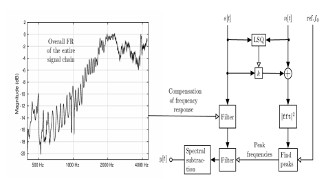
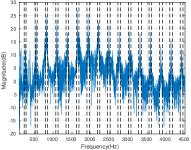
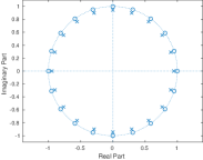
Figure 1: Upper panel: A block diagram of the post-processing algorithm. Here $s[t]$ and $n[t]$ denote the discretised speech and noise samples at $f_{s}=44\,100\,\textrm{Hz}$, respectively. The signal $y[t]$ is de-noised speech. Lower panel on the left: Harmonic structure of the MRI noise and stop bands estimated from it. Lower panel on the right: The zero/pole placement in $z$-plane of the notch filter of degree $20$ for removing the frequency $f_{s}/20$ and its harmonics below the Nyquist frequency $f_{s}/2$.

II-A Arrangements

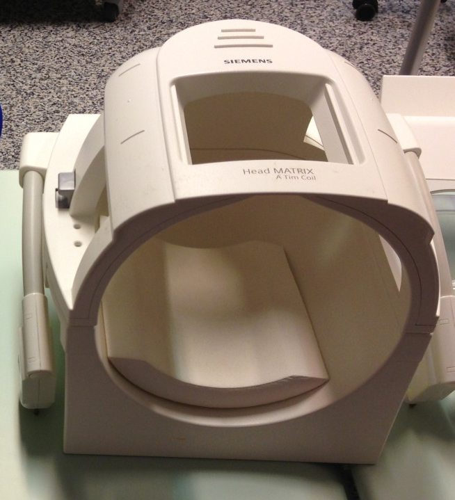
Figure 2: Left panel: The MRI head coil of Siemens Magnetom Avanto 1.5T scanner. The two-channel acoustic sound collector fits exactly the opening on the top. Right panel: The sound collector positioned above a head model similarly as in the MRI experiments. The noise sample is acquired using a horn on the top surface of the collector and the speech sample from another similar horn pointing downwards.

The experimental arrangement has been detailed in [11, 1, 2]. Briefly, a two-channel acoustic sound collector samples speech and MRI noise in a configuration shown in Fig. 2. The signals are acoustically transmitted to a microphone array inside a sound-proof Faraday cage by waveguides of length $3.00$ m. The microphone array contains electret microphones of type Panasonic WM-62. The preamplification and A/D conversion of the signals is carried out by conventional means, see [2, Section 3.1]. The experiments were carried out using Siemens Magnetom Avanto 1.5T using 3D VIBE (Volumetric Interpolated Breath-hold Examination) MRI sequence [58] as it allows for sufficiently rapid static 3D acquisition. Imaging parameters, etc., have been described in [2, Section 3.2].

II-B Phonetic and geometric materials

The speech materials consist of Finnish vowels [, e, i, o, u, y, æ, œ] that were pronounced by a 26-year-old healthy male (in fact, the first author) in supine position during the MRI. The number of samples varies between 3 and 9 depending on the vowel. The MRI sequence requires up to $11.6$ s of continuous articulation in a stationary supine position. The test subject produced the vowels at a fairly constant fundamental frequency $f_{0}$, given by the cue signal to the earphones. Two different pitches $f_{0}=104\,\mathrm{Hz}$ and $f_{0}=130\,\mathrm{Hz}$ were used, and they had been chosen so as to avoid spectral peaks of the MRI noise.

The paired MRI/speech data for this article was acquired during a single session of $82$ min. in the MRI laboratory using the protocols reported in [1, 2]. We obtained $107$ MRI scans which is only possible using well-optimised experimental arrangements. Of the $107$ scans, no more than $36$ were prolonged vowels at $f_{0}\approx 104\,\mathrm{Hz}$ (with sample lengths $\approx 11.2\,\mathrm{s}$) deemed usable for this study. To obtain comparison data, same kind of speech recordings were carried out in the anechoic chamber but neither the MRI coil reflections nor the ambient noise were replicated. Compared to MRI experiments, there are no similar restrictions in the anechoic chamber, apart from test subject fatigue. Thus, each vowel was now produced $10$ times since the larger sample number was possible as a benefit of less demanding experimental arrangement.

III MRI noise cancellation

We treat the measurement signals from speech and acoustic MRI noise $s[t]$ and $n[t]$ for $t\in\{h,2h,3h,\ldots\}$ in their digitised form where $h=1/f_{s}$, and the sampling frequency $f_{s}=44\,100\,\textrm{Hz}$. The post-processing algorithm for these discrete time signals is outlined in Fig. 1 (upper panel), and it consists of the following Steps 1–6 that have been realised as MATLAB code:

1. LSQ: Speech channel crosstalk is optimally removed from noise signal using coefficient $k$ from least squares minimisation.

2. Frequency response compensation: The frequency response of the whole measurement system, shown in Fig. 1 (upper panel), is compensated. The peaks in the frequency response are due to the longitudinal resonances of the waveguides, used to convey the sound from inside the MRI scanner to the microphone array placed in a sound-proof Faraday cage.

3. Noise peak detection: The noise power spectrum is computed by FFT, and the most prominent spectral peaks of noise are detected.

4. Harmonic structure completion: The set of noise peaks is completed by its expected harmonic structure to ensure that most of the noise peaks have been found as shown in Fig. 1 (lower panel on the left). There are heuristics involved so that the harmonics of the reference value of $f_{0}$ do not get accidentally removed. Details are described below in pseudocode.

5. Notch filtering: The noise peaks are removed by using notch filters provided by the MATLAB function iircomb with parameters n equal to the number of different harmonic overtone structures detected, and the $-3\,\textrm{dB}$ bandwidth bw set at $6\cdot 10^{-3}$.

6. Spectral subtraction: A sample of the acoustic background (including, e.g., noise from the helium pump) of the MRI laboratory (without patient speech and scanner noise) is extracted from the beginning of the speech recording. Finally, the averaged spectrum of this “silent sample” is subtracted from the speech signal using FFT and inverse FFT; see [12].

We associate with each spectral peak $p$ its location in spectrum $loc(p)$ in $Hz$, and its height $mag(p)$ in $dB$.

Algorithm 1 Adaptation to spectral structure

1:$P\leftarrow$ set of all peaks found in the spectrum.

2:procedure FindHarmonics(P)

3:     while $P\neq\emptyset$ do

4:         $p\leftarrow\max_{mag}P$

5:         $P\leftarrow P\setminus p$

6:         for $q\leftarrow P$ sorted by $|loc(p)-loc(P)|$ do

7:              $d\leftarrow|loc(p)-loc(q)|$

8:              if $d<cf_{0}$ then

9:                  continue               

10:              if $\exists$ harmonics with fundamental $d$ then

11:                  $F\leftarrow F\cup$ iircomb$(f_{s}/d)$

12:                  $P\leftarrow P\setminus\{r\in P\,:\,r=nd,n\in\mathbb{Z}\}$                             

13:     return F

Harmonics are considered successfully found at step 10, if $P$ contains four consecutive peaks with distance $d$. The value $1.5$ has been used for the parameter $c$.

The proposed approach differs essentially from the earlier approach proposed in [2, Section 4]. Firstly, now there is no direct time-domain subtraction of the measured noise component from speech which makes the present approach more similar to [5]. For that reason, the low frequency components of speech are not attenuated as a result of the proximity of recording sound effect in dipole configurations. Secondly, using notch filters instead of high-order Chebyshev produces sharper removal of unwanted spectral components with much reduced musical noise artefact compared to what was reported in [2]. The comb filter is a more efficient way of removing higher harmonics of spectral peaks in the entire spectrum. In the current approach, the filter degree is determined by the Nyquist frequency $f_{s}/2=22\,050\,\mathrm{Hz}$ and the number of notches required, making the computations much less intensive. However, using Chebyshev filters made it possible to vary the bandwidth of the stop bands as a function of frequency which possibility is now lost.

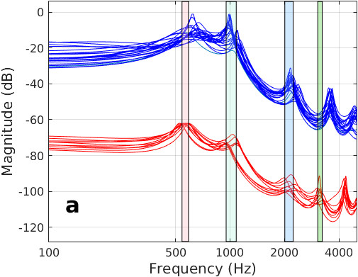
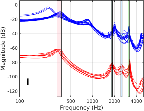
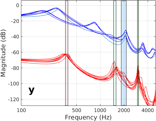
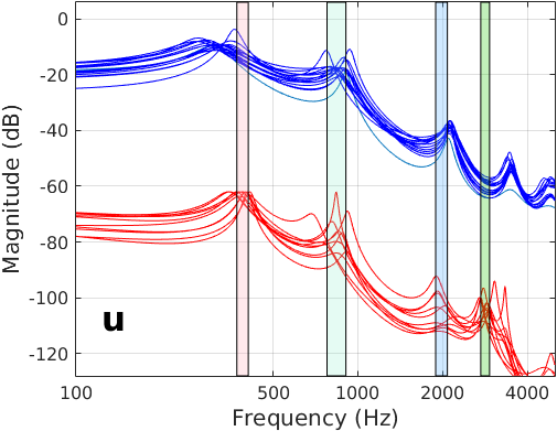
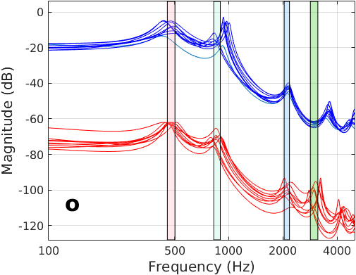
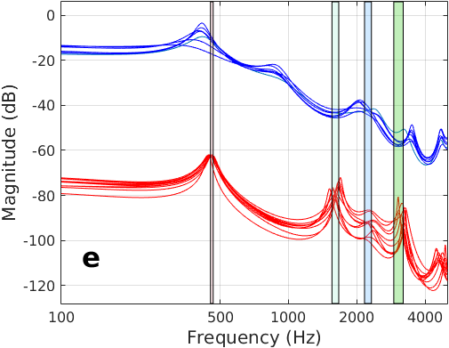
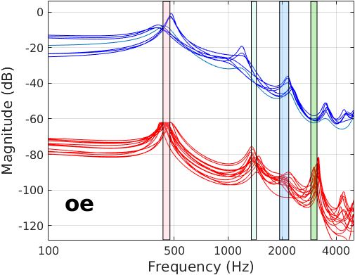
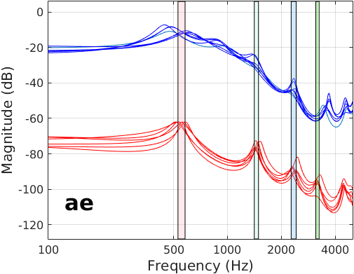
Figure 8: Spectral envelopes of all vowel samples in the dataset. In each panel, the upper curves represent post-processed signals recorded during the MRI experiments. The lower curves are similar envelopes without any post-processing of signals, obtained from the same test subject in the anechoic chamber. These two families of curves are comparable to curves given in [2, Figs. 7–8]. The vertical bars are error intervals for formants $F_{1},\ldots,F_{4}$ extracted from the recordings in the anechoic chamber.

In [2], the post-processed speech recordings during MRI were classified with linear discriminant classifier, using the speech recorded in the anechoic chamber as a learning set. This experiment yielded 62% correct classifications. Repeating the experiment using the same speech data, the improved post-processing algorithm, and better accounting for the strong exterior resonance at $\approx 1kHz$ as discussed in Section VI below, the proportion of correctly classified vowels increases to 72%. Further significant improvement in classification accuracy does not seem possible since a strong systematic component is present in classification errors of both classification experiments, reflecting the properties of the speech data. More precisely, many [æ] get classified as [e], and many [e] get classified as [i]. Looking at the spectral envelopes of [æ] in Fig. 8, two different kinds of behaviour can be seen in the upper curves. Based on only $F_{1}$ and $F_{2}$, samples with the lower first peak location (i.e., $F_{1}[$æ$]$) are almost indistinguishable from [e] recorded in the anechoic chamber. This results in the first kind of systematic error. The second type of error is due to the systematic overestimation of $F_{2}[{\tipaencoding e}]\approx 2\,\mathrm{kHz}$ in speech recorded during MRI as can be seen in Fig. 6. This artefact is connected to the acoustics inside the MRI head coil in Sections V and VI.

IV Performance analysis

IV-A Validation through synthetic signals

The formant extraction from noisy speech can validated using artificially noise contaminated speech where the original formant positions are known precisely. Pure vowel signals were taken from comparison data for each vowel in [, e, i, o, u, y, æ, œ], and their formants $F_{1},F_{2}$, and $F_{3}$ were computed. A sample of MRI noise (without any speech content) was recorded using the experimental arrangement detailed in [2, Section 3], and it was mixed with each vowel sample so that the speech and noise components have equal energy contents ($\mathrm{SNR}\approx 0\,\mathrm{dB}$). The post-processing algorithm described in Section III was then applied to these signals, of which an example is shown in Fig. 3.

It was first observed that the post-processing increases the SNR of the artificially noise-contaminated signals by $9\ldots 14\,\mathrm{dB}$ depending on the vowel. The three formants $F_{1},F_{2}$, and $F_{3}$ were extracted from artificially noise contaminated vowels after they had been post-processed. The resulting formant frequencies are within $-0.5\ldots 0.3$ semitones from those measured from the original pure vowels, except for the outlier $F_{2}$[o] where the discrepancy is $1.1$ semitones.

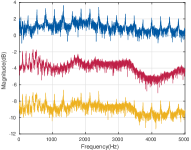
Figure 3: Illustration of the artificially noise-contaminated vowel signal. On the left, MRI noise (upmost), pure vowel signal (middle), and the synthetic signal as their sum (lowest). On the right, synthetic signal (upmost), signal after post-processing using the proposed algorithm (middle), and the reconstructed noise (lowest).

Vowel $F_{1}$ $F_{2}$ $F_{3}$ [] 598 1094 1918 [e] 453 1691 2255 [i] 318 1900 2097 [o] 465 815 2233 [u] 410 898 1934 [y] 379 1535 2034 [æ] 562 1452 2375 [œ] 436 1400 2076 Vowel $F_{1}$ $F_{2}$ $F_{3}$ [] 615 1129 2021 [e] 443 1714 2299 [i] 327 1909 2293 [o] 451 858 2088 [u] 416 921 2041 [y] 390 1533 2015 [æ] 559 1476 2319 [œ] 428 1421 2099

TABLE I: Original formants (left) and formants extracted after the artificial addition of MRI noise and subsequent noise cancellation (right).

The average formant discrepancies of under $2.8$ semitones were reported in [2, Table 3] between speech formants and Helmholtz resonances computed from vocal tract geometries (without any model for the surrounding space) that were obtained by simultaneous MRI. Also, the observations in [14] provide magnitudes for formant error that results from inherent variation in long vowel productions due to test subject adaptation and fatigue. Comparing these values with the results on artificially contaminated speech, we conclude that formant extraction from algorithmically post-processed signals can be regarded as a relatively small error source.

IV-B Comparison of spectral tilts

In addition to formants, another important spectral characteristic of speech signals is the spectral tilt or roll-off. It is a measure of attenuation at higher frequencies that are still relevant to speech. We quantify the spectral tilt by first fitting a low-order rational spectral envelope on the frequency range of speech, and then finding the LSQ regression line to the envelope on the logarithmic frequency range between $465\,\mathrm{Hz}$ and $5\,\mathrm{kHz}$. The bound $465\,\mathrm{Hz}$ is the mean of all $F_{1}$’s present in the dataset.

[] [e] [i] [o] [u] [y] [æ] [œ] Anech 12.2 11.9 9.0 14.5 15.6 12.6 11.3 12.7 MRI 15.7 13.9 9.2 17.9 15.3 13.5 14.0 15.2

TABLE II: Spectral tilts (in $\mathrm{dB}/\mathrm{octave}$) from recordings in the anechoic chamber and from samples recorded during the MRI noise after post-processing.

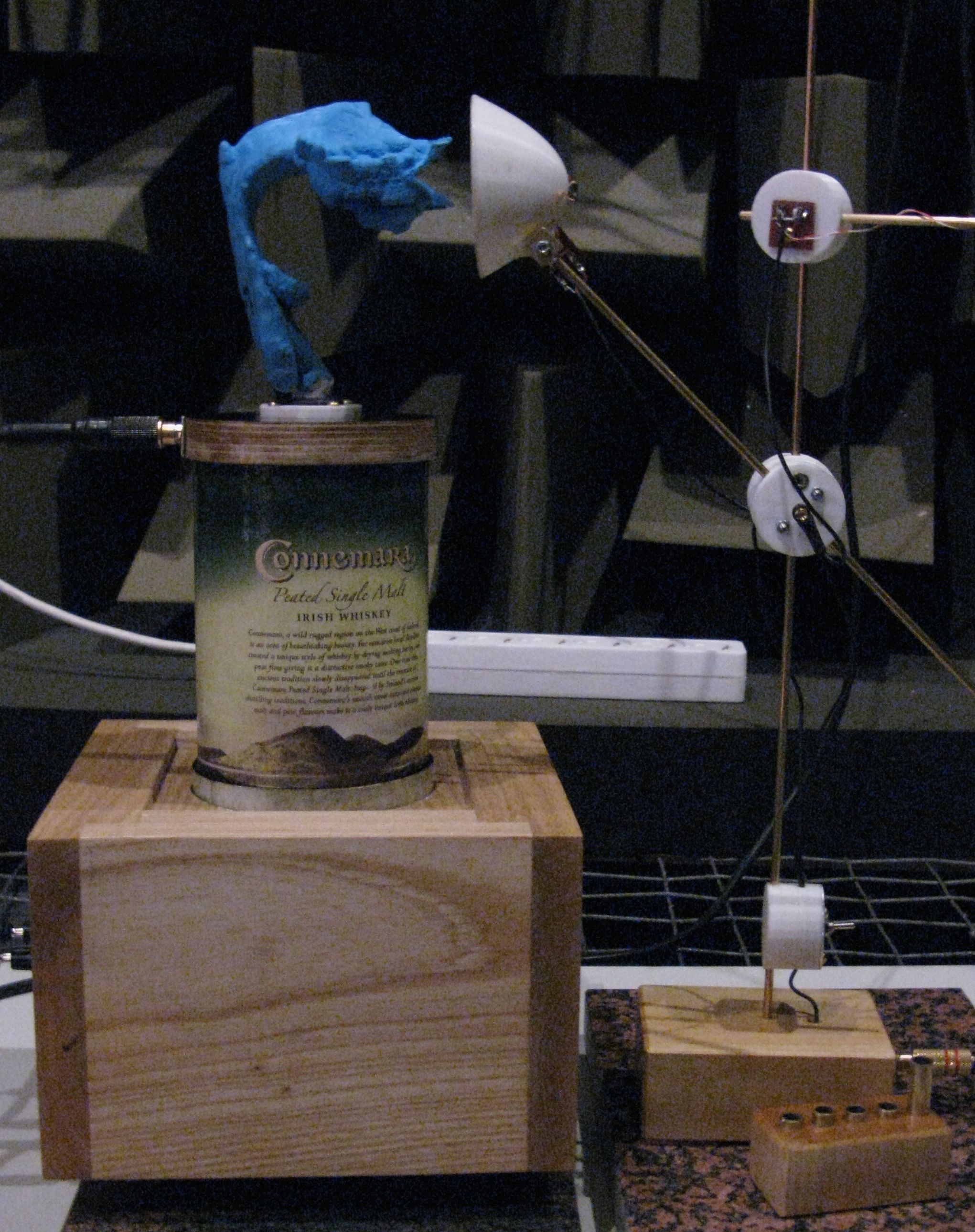
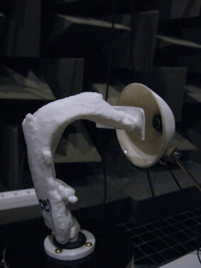
Figure 4: A detail of the sweep measurement arrangement for 3D printed vocal tract configurations of [, œ].

The spectral tilt data is given in Table II. The roll-off in post-processed speech during the MRI is systematically larger than in comparison data (in average by $1.9\,\mathrm{dB}$), the only exception being the vowel [y]. We point out that the two kinds of spectral tilt data in Table II correlate strongly ($R=0.78$). As can be seen from Fig. 5 (last panel), the difference of the average spectral tilts is quite small. The difference is partly explained by the fact that there was a lot of more attenuating material around the test subject in the MRI scanner, compared to experiments in the anechoic chamber.

IV-C Comparison to sweeps in physical models

Three of the MR images corresponding to Finnish quantal vowels [, i, u] were processed into 3D surface models (i.e., STL files) and intersectional area functions for Webster’s equation as explained in [15]. Fast prototyping was used to produce physical models from the STL files in ABS plastic with wall thickness $2\,\mathrm{mm}$. The printed models extend from the glottal position to the lips, and they were coupled to a custom acoustic source (see Fig. 4) whose design resembles the loudspeaker-horn construction shown in [16, Fig. 1]; see also [17].

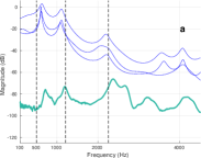
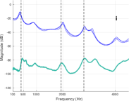
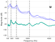
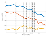
Figure 5: The first three panels: Spectral envelopes and computationally obtained resonances of [, i, u]. The upper curves are power spectral densities of speech recorded during an MRI scan. The lower curves are frequency responses measured from the physical models that have been produced from the MR images. The vertical lines indicate the three lowest resonances computed by Webster’s model from the same VT geometry using the mouth impedance optimisation process introduced in [9]. The last panel: Averages of spectral envelopes of Finnish vowels [, e, i, o, u, y, æ, œ] from two different kind of recordings. Each vowel appears in the averages with the same weight. The topmost curve describes speech recorded during the MRI scan, the middle curve recordings in the anechoic chamber, and the lowest curve is their difference. The averaging highlights the common features (partly due to the exterior acoustics) within both kinds of vowel recordings. The vertical dashed lines represent $k$-means cluster centroids of the Helmholtz resonant frequencies computed using a 3D model of the MRI head coil.

The acoustic source contains an electret (reference) microphone ($\oslash\,9\,\mathrm{mm}$, biased at $5\,\mathrm{V}$) at the glottal position, and another similar (signal) microphone was placed near the lips. A sinusoidal logarithmic sweep was preweighted by the iteratively measured inverse response of the acoustic source in order to obtain a uniform sound pressure level at the reference microphone for all frequencies of interest. The frequency responses of the physical models (and reference resonators with known resonant frequencies were measured using this arrangement between $80\,\mathrm{Hz}\ldots 7\,\textrm{kHz}$.

As can be seen from Fig. 5, there is good correspondence between the spectra of de-noised speech from MRI experiments and the spectra from physical models of the simultaneously imaged vocal tract geometry. There are some extra peaks in both kinds of spectra that correspond to spurious resonances not due to the vocal tract geometry. We point out that the physical models did not contain the face, and the sweep measurements were carried out in an open acoustic environment in the anechoic chamber. This is in contract to the speech recordings that were carried out within MRI head and neck coils [1, 2].

It is worth observing from Fig. 5 that the spectral tilt (as defined in Section IV-B) of the frequency response from physical models is practically $0\,\mathrm{dB}/\mathrm{octave}$. This is due to two reasons: (i) A 3D printed vocal tract is a virtually lossless acoustic system apart from the radiation losses through mouth opening, and (ii) the glottal excitation in natural speech has its characteristic roll-off of $11\ldots 16\,\mathrm{dB}/\mathrm{octave}$ whereas the measurements from the physical models were carried out keeping the sinusoidal sound pressure constant at the glottal position.

IV-D Perceptual evaluation

A listening experiment was carried out to evaluate the effect of post-processing on vowel recognition. In the experiment, $12$ subjects (of which two were female) listened to $48$ recordings of vowel phonation. The recordings consisted of $6$ samples of each Finnish vowel in [, e, i, o, u, æ, œ]; half of the samples were unprocessed recordings from the anechoic chamber ($24$ in total, three for each vowel), while the rest had undergone the MRI noise contamination and de-noising process described in Section IV-A. The duration of each sample was $10\,\mathrm{s}$.

a) Vowel samples from anechoic chamber
categorised as target [] [e] [i] [o] [u] [y] [æ] [œ] $[$ $]$ 36 0 0 0 0 0 0 0 $[$ e $]$ 0 33 0 0 0 0 0 3 $[$ i $]$ 0 0 36 0 0 0 0 0 $[$ o $]$ 6 0 0 30 0 0 0 0 $[$ u $]$ 0 0 0 13 23 0 0 0 $[$ y $]$ 0 0 0 0 0 32 0 4 $[$ æ $]$ 0 1 0 0 0 0 32 1 $[$ oe $]$ 0 3 0 0 0 0 0 33

b) Artificially MRI noise contaminated samples
categorised as target [] [e] [i] [o] [u] [y] [æ] [œ] $[$ $]$ 36 0 0 0 0 0 0 0 $[$ e $]$ 0 30 0 0 0 0 0 6 $[$ i $]$ 0 0 36 0 0 0 0 0 $[$ o $]$ 8 0 0 28 0 0 0 0 $[$ u $]$ 0 0 0 15 21 0 0 0 $[$ y $]$ 0 0 0 0 0 27 0 9 $[$ æ $]$ 0 0 0 0 0 0 36 0 $[$ oe $]$ 0 0 0 1 0 0 0 35

TABLE III: Results of the perceptual comparison experiment on vowels, some of which were artificially contaminated by MRI noise and then de-noised. Quite many target samples of [u] were classified as [o] in both kinds of samples.

The test subjects were allowed to listen each sample as many times as they wanted. Using a computer interface, they reported the vowel that the phonation resembled the most in their opinion. The results of the perceptual experiment are given in Table III. As a conclusion, there is a slight increase in classification mistakes induced by the proposed algorithm, but the increase is a fraction of the classification mistakes due to natural speech variation in the samples used. To draw statistically significant conclusions on such small effects would require a considerably larger data set.

V Formant extraction from noisy speech

After four validation experiments on the post-processing algorithm described in Section III, it is time to apply it on true speech data, recorded during an MRI scan. Our purpose is to show by comparative studies that the acoustic environment in the MRI scanner introduces resonant artefacts to speech signals that are large enough to be clearly quantifiable using the proposed algorithm.

To increase the number of vowel sound samples from MRI experiments, six partial samples of $1\,\mathrm{s}$ were taken from each recording. These partial samples are separated from each other by at least $1\,\textrm{s}$ of time to enhance the independence of the samples. This sixfold increase of the original sample number improves the statistical analysis given in Table IV. Spectral envelopes of all speech samples are shown in Fig. 8 where variance between same vowel productions in different MRI scans (or different parts of the same scan) can be observed.

We proceed to show that some of the extracted formant means of samples from the anechoic chamber and the MRI laboratory are significantly nonequal. The estimated formant means $\mu_{ac}$ and $\mu_{mri}$ are compared using Student’s t-distribution where the degrees-of-freedom is determined by the Smith-Satterwaithe procedure; see the unequal variance test statistics in, e.g., [19, Section 10.4]. In case of the vowel formant $F_{j}$[] for $j=1,2,3$, our null hypothesis is that

$$H_{0}:\mu_{ac}\left(F_{j}\text{[{\tipaencoding\textscripta}]}\right)=\mu_{mri}\left(F_{j}[\text{{\tipaencoding\textscripta}]}\right)$$

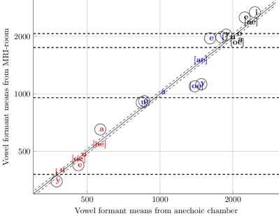
Figure 6: Estimates of formants $F_{1}$, $F_{2}$, and $F_{3}$ that have been extracted from the vowel samples of [, e, i, o, u, y, æ, œ] recorded during the MRI. They are plotted against the comparable data recorded in the anechoic chamber from the same test subject. The diagonal dashed lines describe the error bounds of $\pm 0.5$ semitones as obtained in Section IV-A. Where the formant discrepancy is statistically significant at $p\geq 0.95$, the vowel has been encircled; see Table IV. The horizontal dashed lines show peaks of the spectral envelopes in Fig 5 (last panel) that were identified as resonances external to the vocal tract.

We try to reject $H_{0}$ by showing that its converse $H_{1}$ is true with high probability, say $p>0.95$, in which case the experiment indicates that the formant extraction from the two data sources is not consistent. The results of the experiments are given in Table IV where the $p$-values are given. We conclude that $H_{0}$ gets typically rejected for $F_{2}$ in all vowels except [, o, æ] and for all formants in vowels [e, i].

The formant means from post-processed speech during the MRI are plotted in Fig. 6 against their counterparts recorded in the anechoic chamber from the same test subject. If these two datasets were perfectly consistent, all data points would be expected to appear between the two diagonal dashed lines, representing the maximum error of formant extraction from noisy speech as discussed in Section IV-A. We conclude that (at least) 12 of the discrepancies shown in Fig. 6 reflect actual differences of the speech data recorded in MRI laboratory, compared to similar data from the anechoic chamber.

It is worth observing that the formant discrepancy in Fig. 6 shows a peculiar staircase pattern where two plateaus appear near $1\,\textrm{kHz}$ and $2\,\textrm{kHz}$. More precisely, we observe that in samples recorded during the MRI, we have $F_{2}$[y], $F_{2}$[œ] $\to 1\,\mathrm{kHz}$ from above and $F_{2}$[e], $F_{2}$[i] $\to 2\,\mathrm{kHz}$ from below. The vertical level at $1\,\textrm{kHz}$ coincides with an extra peak appearing in Fig. 8 in most of spectral envelopes of signals recorded during the MRI; notable exceptions are the vowels [,u,o] where $F_{2}\approx 1\,\textrm{kHz}$ would conceal any extra peak. These extra peaks can also be seen in Fig. 5 (last panel) where the spectral envelopes of all vowel recordings in the MRI laboratory (in the anechoic chamber, respectively) have been averaged to downplay the vowel specific formant peaks. It has been excluded by frequency response measurements and ensuing equalisation that these peaks could be an artefact of the speech recording instrumentation.

[] [e] [i] [o] [u] [y] [æ] [œ] $F_{1}$ 0.99 0.98 0.84 0.14 0.70 0.95 0.25 0.07 $F_{2}$ 0.21 0.99 0.99 0.99 0.98 0.99 0.81 0.98 $F_{3}$ 0.82 0.99 0.99 0.60 0.17 0.99 0.61 0.75

TABLE IV: The $p$-values computed with Smith-Satterwaith procedure for distributions with unequal variances. Formant samples that reject the null hypothesis $H_{0}$ at $p>0.95$ are written in bold.

A similar staircase pattern to Fig. 6 near frequencies $1\,\textrm{kHz}$ and $2\,\textrm{kHz}$ has been observed in [20, Chapter 5, Fig. 5.4] where measured formant and computed resonance pairs have been plotted against each other. The vocal tract resonances in [20] have been computed by the Helmholtz equation from MRI data without exterior space modelling, and the formants have extracted from recordings during the MRI as explained in [2, Section 5].

VI Identification of exterior resonances

The statistically significant discrepancy in Fig. 6 is expected to be a combination of three different sources: (i) Perturbation of the vocal tract resonances by the adjacent exterior space resonances, caused by reflections from test subject’s face and MRI head coil surfaces; (ii) Lombard speech due to the acoustic noise during the MRI (see [21, 22]); and (iii) active adaptation of the test subject to the constrained space acoustics inside the MRI head coil. Of these three possible partial explanations, only the first can be studied without carrying out extensive experiments with test subjects. Instead, we can use the simultaneously obtained MR image of the vocal tract for numerical resonance computations in order to investigate the acoustic artefacts in speech caused by the MRI coil.

We extract the vocal tract geometries from the MR images by custom software as explained in [20]. The vocal tract geometries are joined with an idealised geometric model of the head coil as well as a head geometry as shown in Fig. 7. The head geometry was purchased from TurboSquid [18]. The computational domain $\Omega$ is split into the interior part $\Omega_{1}$, the exterior part $\Omega_{2}$, and the spherical interface $\Gamma=\partial\Omega_{1}\cap\partial\Omega_{2}$ as shown in Fig. 7. Both $\Omega_{2}$ and $\Gamma$ are same in all computations but $\Omega_{1}$ (containing the vowel dependent vocal tract) changes.

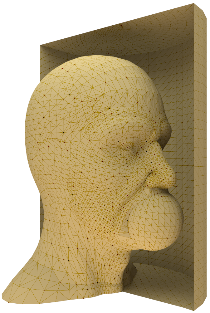
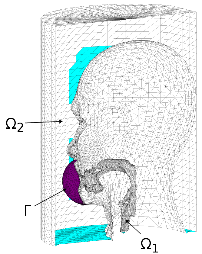
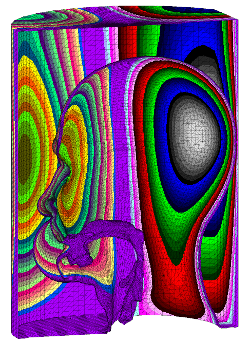
Figure 7: Top panels: An illustration of the computational domains used for identifying the acoustic resonances within MRI head coil. The computational domains $\Omega_{1}$, $\Omega_{2}$, and the interface $\Gamma$ are shown on the right. Bottom panel: The modal pressure distribution at the domain boundary at the resonant frequency $1062\,\mathrm{Hz}$.

We use the finite element method (FEM with piecewise linear elements on a tetrahedral mesh with discretisation parameter $h>0$) to solve the Helmholtz equation $\Delta u=\kappa^{2}u$ in $\Omega$ and identify those resonances that have strong excitations in $\Omega_{2}$. Here $\kappa=\omega/c$ where $c$ is the speed of sound, and $\omega$ is the complex angular velocity. Using FEM and Nitsche’s method (see [25]) on the interface $\Gamma$, the Helmholtz equation takes the variational form

$$a(u,v)=\kappa^{2}b(u,v)\quad\textrm{for all }v\in V$$ (1)

where the bilinear form $a(\cdot,\cdot)$ is defined as

$$a(u,v) =\sum_{i=1}^{2}(\nabla u,\nabla v)_{\Omega_{i}}-\left<\left\{\frac{\partial u}{\partial n}\right\},\llbracket v\rrbracket\right>_{\Gamma}$$

$$-\left<\llbracket u\rrbracket,\left\{\frac{\partial v}{\partial n}\right\}\right>_{\Gamma}+\nu_{h}\left<\llbracket u\rrbracket,\llbracket v\rrbracket\right>_{\Gamma}.$$

Here $\{u\}$ ($\llbracket u\rrbracket$) is the average (respectively, the jump) of $u$ over the interface $\Gamma$, and $\nu_{h}$ is a mesh size dependent parameter. The bilinear form $b(\cdot,\cdot)$ in (1) is the inner product of $L^{2}(\Omega)$. Using Nitsche’s method on interface $\Gamma$ makes it possible to use the same discretisation of $\Omega_{2}$ for all vowel geometries. For a similar kind of numerical experiment, see [26].

The resonance structures of each of the $51$ vowel geometries in the data set were computed on $\Omega$ by FEM as explained above. The resulting $3060$ complex angular velocities $\omega$ were processed as follows:

1. Depending on the vowel, three or four $\omega$’s, corresponding obviously to the lowest formants of the vocal tract volume $\Omega_{1}$, were excluded. This was based on comparing the energy densities in $\Omega_{1}$ and $\Omega_{2}$ of the respective eigenfunctions $u$. A total of $2866$ $\omega$’s remain that indicate significant acoustic excitation in the exterior domain $\Omega_{2}$.

2. Next, $1075$ of the $2866$ eigenfunctions $u$ having largest $\mathop{Re}{\omega}$ (i.e., being least attenuated) were identified, with frequencies between $300\,\textrm{Hz}\ldots 3\,\textrm{kHz}$.

3. Eight frequency clusters were formed by the $k$-means algorithm (see [24]) from the remaining $1075$ complex wavenumbers $\omega$ based on the resonant frequencies $f=\mathop{Im}{\omega}/2\pi$.

The cluster centroids indicate concentrations of acoustic energy around the eight frequencies, shown by vertical dashed lines in Fig 5. The energy concentrations coincide quite well with the peaks of the topmost curve in Fig. 5 (last panel), produced from speech during the MRI. There is much less match with the middle curve in the same figure, produced from speech in the anechoic chamber. We conclude that some effects of the MRI coil reflections are, indeed, present in speech recorded during the MRI. The corresponding artefact peaks in speech spectrograms occur at the frequencies $380\,\mathrm{Hz}$, $955\,\mathrm{Hz}$, $1750\,\mathrm{Hz}$, $2070\,\mathrm{Hz}$, $3230\,\mathrm{Hz}$, $3970\,\mathrm{Hz}$, and $5090\,\mathrm{Hz}$, of which the four lowest are displayed as horizontal lines in Fig. 6.

VII Conclusions

When trying to match a computational model of speech to true speech biophysics, some sort of paired data is necessary. For example, if the acoustic modelling is based on vocal tract geometries acquired by MRI, then the most suitable accompanying data consists of speech samples recorded during the same MRI scan. Unfortunately, these samples are always contaminated by high levels of scanner noise and other acoustic artefacts that must be eliminated before a reliable extraction of desired features (such as the formant positions and the spectral tilt) is possible. Applications related to, e.g., modelling of oral and maxillofacial surgery require extreme precision that is feasible in model computations only by careful parameter estimation and validation of model components. Such models can only be as reliable as their validation data.

A post-processing algorithm was proposed for removing acoustic noise from speech that has been recorded during the MRI using special MRI-proof instrumentation. It is one of the salient features of MRI scanner noise that it mainly consists of few strong fundamental frequencies accompanied by their harmonic overtones. The algorithm outlined in Section III first identifies such harmonic structure and then adapts a collection of notch filters to the detected frequencies. The algorithm is realised as MATLAB code.

The proposed algorithm is significantly different from the approaches presented in [5, 6, 7, 8]. Many of these differences are motivated by dissimilarities in experimental arrangements for data acquisition. Scanners with lower magnetic field intensity (such as used in [6, 7]) typically have an open construction where speech may be recorded rather successfully by directional microphones, located at a safe distance from the scanner. Low-field scanners unfortunately produce worse image resolution, and they require longer scanning durations which are undesirable features in speech studies. Here, the recording setup is built around a Siemens Magnetom Avanto 1.5T MRI scanner having higher magnetic field intensity but a closed construction. Using the arrangement detailed in Fig. 2, we are able to obtain an accurate estimate of the scanner noise near the test subject’s mouth since the MRI coil surfaces act as an additional acoustic shield between the speech and the noise channels. Thus, the spectral peaks of noise can be extracted quite accurately, and a set of comb filters can be designed to precisely and economically remove these frequency bands from speech recordings. This makes it unnecessary to resort to methods such as the spectral noise gating [8] or the cepstral transformation [6] that affect the entire frequency range. Moreover, the proposed algorithm can make good use of the fact that our main interest lies in long vowel utterances at a fixed $f_{0}$, chosen not to coincide with the dominant spectral peaks of the scanner noise. The zeroes of the comb filters are chosen adaptively for each recording which makes it possible to apply the proposed algorithm to different MRI sequences.

In our measurement setting, speech and noise samples are collected essentially at the same point (see Fig. 2 and [2]) although from opposite directions. Issues related to delays and multiway propagation are less serious compared to settings where the sound is collected further away as was done in [5, 6]. Hence, it is not necessary to develop a high-order noise model as in [5], but a computationally less intensive and a more tractable post-processing of speech can be used.

The proposed algorithm operates almost entirely in frequency domain which is necessary, regardless of all other aspects, for compensating the frequency response of the recording system. We point out that also a real-time, time-domain, analogue subtraction of MRI noise from recorded speech is used during the experiment to provide instant feedback to patient’s earphones. The analogue circuit removes low frequency noise very effectively but is useless at higher frequencies where noise arrives to the sound collector channels in different phase.

The post-processing algorithm was validated by using artificially noise-contaminated vowels where the noise has been recorded from the MRI scanner running the same MRI sequence as in the prolonged vowel experiments. Such artificially MRI noise contaminated vowels have known formant positions and predetermined SNR’s which makes it possible to assess the achievable noise reduction in post-processing. In the proposed approach, we observe that $9\ldots 14\,\textrm{dB}$ reduction of MRI scanner noise is attainable for prolonged vowel signals, and the formant extraction error due to post-processing is less than half a semitone. This is an adequate level of performance for the validation and the parameter estimation of a computational speech model such as proposed in [3].

The algorithm was applied on real speech data. A set of prolonged vowels was recorded during the MRI, and this data was post-processed. Comparison measurements were recorded in optimal conditions from the same test subject. Vowel formants were extracted from both types of data, and it was observed that the formant discrepancy between the two kinds of data has a strongly frequency dependent behaviour. Particularly large deviations were observed near $1\,\textrm{kHz}$ and $2\,\textrm{kHz}$. At these frequencies, the formant discrepancy is several times as large as the formant estimation error due to the post-processing algorithm, and the deviations are statistically significant (Student’s t-test with $p>0.95$). We presented computational evidence that the deviant frequencies are related to the acoustic resonances of the space between test subject’s face and MRI coils. However, some of the formant error may also be due to test subject’s adaptation to his acoustic environment during the MRI scan.

The notch filtering adds a large number of transmission zeros to processed signals which causes the phase response of the algorithm to be non-linear. This may be a showstopper if the post-processed signal is to be used as an input for another speech processing algorithm such as the Glottal Inverse Filtering (GIF) for glottal pulse extraction, see [27, 28]. To produce signals with linear phase response, one should use, e.g., non-causal spectral filtering (see [23]) instead of notch filters.

Even though the algorithm has been designed for the main purpose of formant extraction, it gives audibly quite satisfactory results from natural speech that has been recorded during dynamic MRI of mid-sagittal sections.

References

- [1] D. Aalto, O. Aaltonen, R.-P. Happonen, J. Malinen, P. Palo, R. Parkkola, J. Saunavaara, and M. Vainio, “Recording speech sound and articulation in MRI,” in Proceedings of BIODEVICES, 2011, pp. 168–173.
- [2] D. Aalto, O. Aaltonen, R.-P. Happonen, P. Jääsaari, A. Kivelä, J. Kuortti, J. M. Luukinen, J. Malinen, T. Murtola, R. Parkkola, J. Saunavaara, and M. Vainio, “Large scale data acquisition of simultaneous MRI and speech,” Applied Acoustics, vol. 83, no. 1, pp. 64–75, 2014.
- [3] A. Aalto, T. Murtola, J. Malinen, D. Aalto, and M. Vainio, “Modal locking between vocal fold and vocal tract oscillations: Simulations in time domain,” arXiv:1506.01395, 2015, submitted.
- [4] A. Hyvärinen and E. Oja, “Independent Component Analysis: Algorithms and Applications,” Neural Networks, vol. 13, no. 4–5, pp. 411–430, 2000.
- [5] E. Bresch, K. Nielsen, K. Nayak, and S. Narayanan, “Synchronized and noise-robust audio recordings during realtime magnetic resonance imaging scans,” Journal of the Acoustical Society of America, vol. 120, no. 4, pp. 1791–1794, 2006.
- [6] J. Přibil, J. Horáček, and P. Horák, “Two methods of mechanical noise reduction of recorded speech during phonation in an MRI device,” Measurement science review, vol. 11, no. 3, pp. 92–99, 2011.
- [7] J. Přibil, A. Přibilová, and I. Frollo, “Analysis of spectral properties of acoustic noise produced during magnetic resonance imaging,” Applied Acoustics, vol. 73, no. 8, pp. 687–697, 2012.
- [8] J. Inouye, S. Blemker, and D. Inouye, “Towards undistorted and noise-free speech in an MRI scanner: correlation subtraction followed by spectral noise gating,” Journal of the Acoustical Society of America, vol. 135, no. 3, pp. 1019–1022, 2014.
- [9] J. Kuortti, J. Kivi, J. Malinen, and A. Ojalammi, “Mouth impedance optimisation for vocal tract resonances of vowels,” in Proceedings of 27th Nordic Seminar on Computational Mechanics, 2015, pp. 93–96.
- [10] J. Palo, D. Aalto, O. Aaltonen, R.-P. Happonen, J. Malinen, J. Saunavaara, and M. Vainio, “Articulating Finnish vowels: Results from MRI and sound data,” Linguistica Uralica, vol. 48, no. 3, pp. 194–199, 2012.
- [11] J. Palo, “A wave equation model for vowels: Measurements for validation.” Licentiate Thesis, Aalto University School of Science, Department of Mathematics and Systems Analysis, 2011.
- [12] S. Boll, “Suppression of acoustic noise in speech using spectral subtraction,” Acoustics, Speech and Signal Processing, IEEE Transactions on, vol. 27, no. 2, pp. 113 – 120, 1979.
- [13] X. Shou, X. Chen, J. Derakhsan, T. Eagan, T. Baig, S. Shvartsman, J. Duerk, and R. Brown, “The suppression of selected acoustic frequencies in MRI,” Applied Acoustics, vol. 71, pp. 191–200, 2010.
- [14] D. Aalto, J. Malinen, M. Vainio, J. Saunavaara, and J. Palo, “Estimates for the measurement and articulatory error in MRI data from sustained vowel phonation,” in Proceedings of the International Congress of Phonetic Sciences, 2011, pp. 180–183.
- [15] D. Aalto, J. Helle, A. Huhtala, A. Kivelä, J. Malinen, J. Saunavaara, and T. Ronkka, “Algorithmic surface extraction from MRI data: modelling the human vocal tract,” in Proceedings of BIODEVICES, 2013, pp. 257–260.
- [16] D. Tze Wei Chu, K. Li, J. Epps, J. Smith, and J. Wolfe, “Experimental evaluation of inverse filtering using physical systems with known glottal flow and tract characteristics,” Journal of the Acoustical Society of America, vol. 133, no. 5, 2013.
- [17] H. Takemoto, P. Mokhtari, and T. Kitamura, “Acoustic analysis of the vocal tract during vowel production by finite-difference time-domain method,” Journal of the Acoustical Society of America, vol. 128, no. 6, pp. 3724–3738, 2010.
- [18] “Head + morph targets 3D model,” Turbosquid, New Orleans, LA, available online at http://www.turbosquid.com/3d-models/ 3d-model-male-head-morph-targets/261694, 2005 (Last viewed 9 June 2016).
- [19] J. Milton and J. Arnold, Introduction to probability and statistics, 4th ed. McGraw-Hill, 2003.
- [20] A. Kivelä, “Acoustics of the vocal tract: MR image segmentation for modelling,” Master’s thesis, Aalto University School of Science, Department of Mathematics and Systems Analysis, 2015.
- [21] V. Hazan, J. Grynpas, and R. Baker, “Is clear speech tailored to counter the effect of specific adverse listening conditions?” Journal of the Acoustical Society of America, vol. 132, no. 5, pp. EL371–EL377, 2012.
- [22] M. Vainio, D. Aalto, A. Suni, A. Arnhold, T. Raitio, H. Seijo, J. Järvikivi, and P. Alku, “Effect of noise type and level on focus related fundamental frequency changes,” in INTERSPEECH, 2012, pp. 1–4.
- [23] W. R. Gardner and B. Rao, “Noncausal all-pole modeling of voiced speech,” Speech and Audio Processing, IEEE Transactions on, vol. 5, no. 1, pp. 1–10, 1997.
- [24] J. B. MacQueen, “Some Methods for classification and Analysis of Multivariate Observations,” Proceedings of 5th Berkeley Symposium on Mathematical Statistics and Probability vol. 1 pp. 281–297, 1967.
- [25] R. Becker, P. Hansbo, R. Stenberg, “A finite element method for domain decomposition with non-matching grids,” ESAIM: Mathematical Modelling and Numerical Analysis, vol. 37, no. 2, pp. 209-225, 2003.
- [26] M. Arnela, O. Guasch, F. Alías “Effects of head geometry simplifications on acoustic radiation of vowel sounds based on time-domain finite-element simulations,” Journal of Acoustical Society of America, vol. 134, no. 4, pp. 2946-2954, 2013.
- [27] P. Alku, “Glottal inverse filtering analysis of human voice production - a review of estimation and parameterization methods of the glottal excitation and their applications,” Sadhana, vol. 36, no. 5, pp. 623–650, 2011.
- [28] ——, “Glottal wave analysis with pitch synchronous iterative adaptive inverse filtering,” Speech Communication, vol. 11, no. 2–3, pp. 109–118, 1992.