Rational quintics in the real plane

Abstract

From a topological viewpoint, a rational curve in the real projective plane is generically a smoothly immersed circle and a finite collection of isolated points. We give an isotopy classification of generic rational quintics in $\mathbb{RP}^{2}$ in the spirit of Hilbert’s 16th problem.

1 Introduction

1.1 Smooth real curves in the plane and Hilbert’s 16th problem

Topological classification of smooth real algebraic curves is one of the most classical problems in real algebraic geometry. It was included by D. Hilbert [8] into his famous list of problems made at the dawn of the XXth century. Let us recall this problem as well as the basic conventions related to it.

Problem 1.1 (Modern interpretation of Hilbert’s 16th problem, Part I, cf. [25]).

Given an integer number $d>0$, describe possible topological types of the pair $(\mathbb{RP}^{2},{\mathbb{R}}C)$, where ${\mathbb{R}}C\subset\mathbb{RP}^{2}$ is the real point set of a smooth algebraic curve of degree $d$ in the real projective plane $\mathbb{RP}^{2}$.

By a real algebraic curve $C$ in $\mathbb{RP}^{2}$ we mean a real homogeneous polynomial in $3$ variables which is considered up to multiplication by a non-zero real constant. Such a polynomial has a zero locus ${\mathbb{R}}C\subset\mathbb{RP}^{2}$ (called the real point set of $C$) and a zero locus ${\mathbb{C}}C\subset\mathbb{CP}^{2}$ (called the complex point set of $C$, or complexification of ${\mathbb{R}}C$). By abuse of language, speaking about a real algebraic curve $C$ in $\mathbb{RP}^{2}$, we often mention only the real point set ${\mathbb{R}}C$.

The degree of a real algebraic curve $C$ in $\mathbb{RP}^{2}$ is the degree of a polynomial defining $C$. A real algebraic curve in $\mathbb{RP}^{2}$ is called non-singular or smooth, if a polynomial defining this curve does not have critical points in ${\mathbb{C}}^{3}\setminus\{0\}$. The real point set ${\mathbb{R}}C\subset\mathbb{RP}^{2}$ of a non-singular curve $C$ is either empty or a smooth $1$-dimensional submanifold of $\mathbb{RP}^{2}$, that is, a disjoint union of $l$ copies of the circle $S^{1}$. Furthermore, by Harnack’s inequality [7] we have $l\leq\frac{(d-1)(d-2)}{2}+1$, where $d$ is the degree of $C$. Notice that $\frac{(d-1)(d-2)}{2}$ is the genus of the complexification ${\mathbb{C}}C\subset\mathbb{CP}^{2}$.

If $d$ is even, then every connected component $Z\subset{\mathbb{R}}C$ is homologically trivial in $\mathbb{RP}^{2}$. Such a component is called an oval. The complement $\mathbb{RP}^{2}\setminus Z$ consists of two open domains: the one homeomorphic to a disk is called the interior of $Z$, the one homeomorphic to a Möbius band is called the exterior of $Z$.

If $d$ is odd, then all but one connected components of ${\mathbb{R}}C$ are ovals. The remaining component $Y\subset{\mathbb{R}}C$ is isotopic to a line $\mathbb{RP}^{1}\subset\mathbb{RP}^{2}$ and is called a pseudoline. The complement $\mathbb{RP}^{2}\setminus Y$ is connected, so we cannot talk of interior or exterior of a pseudoline. Thus, for even $d$ the real point set ${\mathbb{R}}C$ of $C$ consists of $l$ ovals, while for odd $d$ we have one pseudoline and $l-1$ ovals.

There is somewhat more than just the number of ovals in the topology of $(\mathbb{RP}^{2},{\mathbb{R}}C)$. Two ovals $Z,Z^{\prime}$ are called disjoint if their interiors are disjoint in the set-theoretical sense. Otherwise, they are called nested. More generally, we say that a collection of ovals is a nest if any pair of ovals in this collection is nested. The depth of a nest is the total number of ovals in the collection. We say that an oval $Z^{\prime}$ is inside of an oval $Z$ if $Z^{\prime}$ is contained in the interior of $Z$. The oval is called empty if there are no ovals inside of it.

The topology of $(\mathbb{RP}^{2},{\mathbb{R}}C)$ is completely determined by the number of ovals together with information on each pair of ovals whether they are disjoint or one is inside of the other. From a combinatorial viewpoint this information is encoded with a rooted tree whose vertices are connected components of $\mathbb{RP}^{2}\setminus{\mathbb{R}}C$ and whose edges are the ovals of ${\mathbb{R}}C$. The root of this tree is placed at the only non-orientable component of $\mathbb{RP}^{2}\setminus{\mathbb{R}}C$ if $d$ is even and the only component adjacent to the pseudoline if $d$ is odd.

These rooted trees, and thus the topology of $(\mathbb{RP}^{2},{\mathbb{R}}C)$, are traditionally encoded with the following system of notations introduced in [22]. The symbol $J$ stands for a pseudoline. An oval is denoted with $1$. Each rooted tree is bordered with brackets $<>$. E.g. the topological type of a line $\mathbb{RP}^{1}\subset\mathbb{RP}^{2}$ is denoted with $<J>$, and the topological type of an ellipse is denoted with $<1>$.

The notations are built inductively. Let $Z_{1},\dots,Z_{m}$ be the non-empty ovals adjacent to the rooted component of the complement of $\mathbb{RP}^{2}\setminus{\mathbb{R}}C$. The intersection of ${\mathbb{R}}C$ with the interior of $Z_{k}$ can itself be considered as an arrangement of ovals which is already encoded by $<x_{k}>$ with some symbolic notations $<x_{k}>$ by induction.

The topological type of $(\mathbb{RP}^{2},{\mathbb{R}}C)$ is denoted with

$$<J\sqcup a\sqcup 1<x_{1}>\sqcup\dots\sqcup 1<x_{m}>>\quad\text{or}\quad<a\sqcup 1<x_{1}>\sqcup\dots\sqcup 1<x_{m}>>,$$

depending whether ${\mathbb{R}}C$ contains a pseudoline or not (i.e., whether $d$ is odd or even). Here, $a$ is the number of empty ovals adjacent to the rooted component of $\mathbb{RP}^{2}\setminus{\mathbb{R}}C$. The symbol $\sqcup$ is interpreted as a commutative operation, i.e., we do not distinguish $<x_{1}>\sqcup<x_{2}>$ from $<x_{2}>\sqcup<x_{1}>$. The empty curve is denoted with $<0>$.

The following two examples were the starting point for the classification quest known already in the XIXth century.

Example 1.2.

There are $6$ topological types of non-singular curves of degree 4 in $\mathbb{RP}^{2}$. These are $<\alpha>$, where $0\leq\alpha\leq 4$, and $<1<1>>$.

Example 1.3.

There are $8$ topological types of non-singular curves of degree 5 in $\mathbb{RP}^{2}$. These are $<J\ \sqcup\alpha>$, where $0\leq\alpha\leq 6$, and $<J\ \sqcup 1<1>>$.

Real algebraic curves of degree $d$ in $\mathbb{RP}^{2}$ with maximal number of ovals allowed by Harnack’s inequality, i.e., with $\frac{(d-1)(d-2)}{2}+1$ connected components of the real point set, are called $M$-curves, cf. [14]. Note that in degrees 4 and 5 there are unique topological arrangements of $M$-curves: $<4>$ and $<J\sqcup 6>$, respectively.

Definition 1.4 (F. Klein).

A real algebraic curve $C$ in $\mathbb{RP}^{2}$ is said to be of type I if ${\mathbb{R}}C$ is null-homologous in $H_{1}({\mathbb{C}}C;{\mathbb{Z}}_{2})$.

Note that the involution $\operatorname{conj}:{\mathbb{C}}C\to{\mathbb{C}}C$ of complex conjugation has ${\mathbb{R}}C$ as its fixed point set. Therefore, a non-singular real algebraic curve $C$ in $\mathbb{RP}^{2}$ is of type I if and only if ${\mathbb{C}}C\setminus{\mathbb{R}}C$ is disconnected.

It is easy to show that any $M$-curve must have type I. Furthermore, for each degree $d$ there is a curve of type I that has only $[\frac{d}{2}]$ (the integer part of $\frac{d}{2}$) ovals.

Definition 1.5.

A real curve $C$ of degree $d$ in $\mathbb{RP}^{2}$ is called hyperbolic if ${\mathbb{R}}C$ has a nest of depth $[\frac{d}{2}]$.

The Bézout theorem implies that the topological arrangement of the hyperbolic curve is unique: there are no other ovals except for those from the nest of depth $[\frac{d}{2}]$. Indeed, if there is any other oval, then we may draw a straight line through that oval and the innermost oval in the nest. Such a line would intersect all ovals from the nest and the additional oval at least in two points each. This gives $2+2[\frac{d}{2}]>d$ points of intersection between a curve of degree $d$ and a line. In particular, $[\frac{d}{2}]$ is the maximal possible depth of a nest for a curve of degree $d$ in $\mathbb{RP}^{2}$.

It can be shown that all hyperbolic curves are of type I. The complex orientation formula [15] (which is reviewed in Section 3.1) implies the following classical statement which was known already to Klein.

Theorem 1.6.

There are two possible topological types of non-singular curves of degree 4 and type I in $\mathbb{RP}^{2}$: $<4>$ (the $M$-quartic) and $<1<1>>$ (the hyperbolic quartic).

There are three possible topological types of non-singular curves of degree 5 and type I in $\mathbb{RP}^{2}$: $<J\sqcup 6>$ (the M-quintic), $<J\sqcup 1<1>>$ (the hyperbolic quintic), and $<J\sqcup 4>$ (the four-oval quintic of type I).

Currently the classification of topological arrangements of non-singular curves of degree $d$ in $\mathbb{RP}^{2}$ is known up to degree $7$ (Viro [19]). As this classification is rather large, below we list only the possible topological types of $M$-curves. Note that for $d\geq 6$ the topological type of an $M$-curve is no longer unique.

Theorem 1.7 (Gudkov).

There are three possible topological types of non-singular $M$-curves of degree $6$ in $\mathbb{RP}^{2}$: $<9\sqcup 1<1>>$ (the so-called Harnack sextic), $<1\sqcup 1<9>>$ (the so-called Hilbert sextic), and $<5\sqcup 1<5>>$ (the so-called Gudkov sextic).

Theorem 1.8 (Viro).

There are fourteen possible topological types of non-singular $M$-curves of degree $7$ in $\mathbb{RP}^{2}$: $<J\sqcup 15>$ and $<J\sqcup\alpha\sqcup 1<14-\alpha>>$, where $1\leq\alpha\leq 13$.

1.2 Generic rational curves in the plane

This paper is mainly devoted to rational curves in $\mathbb{RP}^{2}$. The complex point set of such a real rational curve of degree $d$ can be described as the image of the map $\varphi:\mathbb{CP}^{1}\to\mathbb{CP}^{2}$ defined by

$$(z_{0}:z_{1})\mapsto(P(z_{0},z_{1}):Q(z_{0},z_{1}):R(z_{0},z_{1})),$$

where $P$, $Q$, $R$ are real homogeneous polynomials of degree $d$ which do not have common zeros in $\mathbb{CP}^{1}$.

A generic rational curve in $\mathbb{RP}^{2}$ is nodal, which means that the only possible singular points of the curve are non-degenerate double points (also called nodes).

We may distinguish three types of nodes of a nodal curve $C$ in $\mathbb{RP}^{2}$: hyperbolic, elliptic and imaginary nodes. Hyperbolic nodes are formed by intersections of pairs of real branches of ${\mathbb{R}}C$. These are points of $\mathbb{RP}^{2}$ such that $C$ is given by $x^{2}-y^{2}=0$ in some local coordinates $(x,y)$ near these points. Elliptic nodes are formed by real intersections of pairs of complex conjugated branches of ${\mathbb{C}}C$. These are points of $\mathbb{RP}^{2}$ such that $C$ is given by $x^{2}+y^{2}=0$ in some local coordinates $(x,y)$ near these points. Finally, imaginary nodes are nodes of $C$ in $\mathbb{CP}^{2}\setminus\mathbb{RP}^{2}$. Such points come in pairs of complex conjugate points. We denote the number of hyperbolic (respectively, elliptic, imaginary) nodes by $h$ (respectively, $e$, $c$).

The following proposition is straightforward.

Proposition 1.9.

The real point set of any nodal rational curve in $\mathbb{RP}^{2}$ is the disjoint union of a circle generically immersed in $\mathbb{RP}^{2}$ and a finite set of elliptic nodes.

Similarly to Hilbert’s 16th problem, one can ask for a topological classification of pairs $(\mathbb{RP}^{2},{\mathbb{R}}C)$, where $C$ is a nodal rational curve of a given degree $d$ in $\mathbb{RP}^{2}$. Since any self-homeomorphism of $\mathbb{RP}^{2}$ is isotopic to the identity, such a topological classification of pairs $(\mathbb{RP}^{2},{\mathbb{R}}C)$ provides an isotopy classification of the real point sets ${\mathbb{R}}C$ of nodal rational curves of a given degree in $\mathbb{RP}^{2}$. The isotopy classification in question is known up to degree $4$ (see [4] and Section 2.5 for details concerning the classification for degree $4$). Among other results related to the isotopy classification of real rational curves, one can mention, for example, the study of maximally inflected real rational curves in the context of the Shapiro-Shapiro conjecture and the real Schubert calculus; see [9]. In this paper we study nodal rational curves of degree $5$ in $\mathbb{RP}^{2}$.

1.3 Classification of generic rational curves of degree $5$

In this section we state our main result, namely the isotopy classification of nodal rational curves of degree $5$ in $\mathbb{RP}^{2}$. The classification is presented below in the form of the list of smoothing diagrams (see Section 2.2 for the precise definitions) of the curves under consideration. Each smoothing diagram describes an isotopy type of a nodal rational curve of degree $5$ in $\mathbb{RP}^{2}$. The isotopy type is obtained by contracting the vanishing cycles (that is, edges) of a smoothing diagram creating a hyperbolic node for each vanishing cycle.

Theorem 1.10.

The isotopy types of nodal rational curves of degree $5$ in $\mathbb{RP}^{2}$ are exactly those listed in the tables 1 – 6.

Remark 1.11.

In tables 2 and 4 we sometimes incorporated several smoothing diagrams in the same picture. The merged smoothing diagrams only differ by the attachment of a single oval by a single edge (drawn with dashed lines). The factor next to these pictures (e.g. $2$x) indicates how many smoothing diagrams are merged.

There are exactly $121$ isotopy types of nodal rational curves of degree $5$ in $\mathbb{RP}^{2}$. With regard to $l,h,e,c$, we get the following numbers of isotopy types:

$c=0$           $l$ $e$ 0 1 2 3 4 5 6 3 13 3 5 24 12 4 1 7 9 9 6 4 2 1 1 $\sum$ 46 24 10 5 2 1 1

$c=2$           $l$ $e$ 0 1 2 3 4 3 7 2 5 8 4 2 1 1 $\sum$ 15 6 2 1 1

$c=4$           $l$ $e$ 0 1 2 3 3 2 1

Additionally, we have exactly one isotopy type for $c=6$ (a non-contractible loop in $\mathbb{RP}^{2}$).

Table 1: Smoothing diagrams of all isotopy types with $c=0,l=3$

Table 2: Smoothing diagrams of all isotopy types with $c=0,l=5$

Table 3: Smoothing diagrams of all isotopy types with $c=0,l=7$

Table 4: Smoothing diagrams of all isotopy types with $c=2,l=3$

Table 5: Smoothing diagrams of all isotopy types with $c=2,l=5$

Table 6: Smoothing diagrams of all isotopy types with $c=4$ (and hence $l=3$) and of the unique isotopy type with $c=6$ (and hence $h=e=0,l=1$)

The parameter $l$ in the above list is the number of connected components of the real part ${\mathbb{R}}C_{\circ}$ of an appropriate small perturbation $C_{\circ}$ of a nodal rational curve $C$ of degree $5$ in $\mathbb{RP}^{2}$ (see Section 5.1). The proof of Theorem 1.10 is presented in Section 5 (restrictions on the topology of nodal rational curves of degree $5$ in $\mathbb{RP}^{2}$) and Section 6 (constructions).

2 Generically immersed curves and their smoothings

2.1 Generically immersed curves instead of smoothly embedded curves

In contrast with smooth curves in the plane, a connected component of an immersed curve may be quite complicated topologically. In the space of all immersions of a circle to the plane (i.e., differentiable maps from $S^{1}$ to the plane such that the differential never vanishes) we may distinguish generic immersions (see below) that only have transverse double points as its self-intersections. This is the only type of singularity of an immersed curve that survives under all small perturbations in the class of smooth maps.

It was noted by V. Arnold [1] that generic immersions of a circle into a plane have some common behaviour with knots in a 3-space, particularly from the viewpoint of finite-type invariants. In conventional knot theory a knot is an embedding of a circle $K\approx S^{1}$ to the 3-space ${\mathbb{R}}^{3}$. Such a knot is commonly depicted with the help of a linear projection $\pi:{\mathbb{R}}^{3}\to{\mathbb{R}}^{2}$ (normally referred to as a vertical projection). The image $\pi(K)$ is immersed to ${\mathbb{R}}^{2}$ and all of its self-crossing points are non-degenerate double points (often called crossings in this context) if the projection $\pi$ is chosen generically. Once we specify at every crossing which of the two branches is above and which is below we get a presentation of a knot by the so-called knot diagram. Different knot diagrams may give the same knot if they are connected with a sequence of the Reidemeister moves for knot diagrams.

Definition 2.1.

Let $X$ be a smooth surface. An immersion $i:S^{1}\to X$ is called generic if all its self-crossing points are non-degenerate double points (called nodes here). Here $S^{1}$ is an oriented circle (e.g. the unit circle in ${\mathbb{C}}$ oriented counterclockwise).

A knot diagram, after forgetting which branch is above and which is below at the nodes, is an example of a generic immersion of a circle in ${\mathbb{R}}^{2}$.

We consider two generic immersions to be equivalent if they are homotopic in the class of generic immersions. Obviously, such equivalence classes are uniquely determined by the isotopy type of $i(S^{1})\subset X$. By abuse of language, we often identify a generic immersion $i:S^{1}\to X$ with its image $K=i(S^{1})$.

Let $T_{1}(X)$ denote the unit tangent bundle of $X$. Using the standard orientation of $S^{1}$ we may lift the immersion $K\subset\ X$ to $\tilde{K}\subset T_{1}(X)$ by associating to each point of the circle $S^{1}$ parameterizing $K$ the unit tangent vector to $K$ according to the orientation. Thus, $\tilde{K}$ is the image of the Gauss-type map $\tilde{i}:S^{1}\to T_{1}(X)$.

Definition 2.2.

The homology class $[\tilde{K}]\in H_{1}(T_{1}(X);{\mathbb{Z}})$ is called the rotation number of $K$ and is denoted with $\operatorname{rot}(K)$.

Example 2.3.

Let us fix an orientation for ${\mathbb{R}}^{2}$ and let $K$ be a positively oriented embedded circle in ${\mathbb{R}}^{2}$. We have $H_{1}(T_{1}({\mathbb{R}}^{2});{\mathbb{Z}})\cong{\mathbb{Z}}$, and we fix the isomorphism by setting $\operatorname{rot}(K)=+1$.

Example 2.4.

We have $H_{1}(T_{1}(\mathbb{RP}^{2});{\mathbb{Z}})\cong{\mathbb{Z}}_{4}$. We fix the isomorphism by setting $\operatorname{rot}(\mathbb{RP}^{1})=1\in{\mathbb{Z}}_{4}$, where $\mathbb{RP}^{1}\subset\mathbb{RP}^{2}$ is a line. Note that there is no need to specify the orientation of this line as the two choices of orientation are isotopic. Thus, if $X=\mathbb{RP}^{2}$, then $\operatorname{rot}(K)\in{\mathbb{Z}}_{4}$. Furthermore, it is easy to see that if $[K]=0\in H_{1}(\mathbb{RP}^{2};{\mathbb{Z}})={\mathbb{Z}}_{2}$, then $\operatorname{rot}(K)$ is even, while if $[K]\neq 0\in H_{1}(\mathbb{RP}^{2};{\mathbb{Z}})={\mathbb{Z}}_{2}$, then $\operatorname{rot}(K)$ is odd.

The following statement is classical.

Theorem 2.5 (Whitney [24]).

Two immersions are homotopic in the class of (not necessarily generic) immersions if and only if their rotation numbers coincide.

It is easy to see that if two generic immersions are homotopic in the class of (not necessarily generic) immersions, then they are obtained from each other by a series of the following planar immersion counterparts of two of the knot theory Reidemeister moves: namely, the second and the third Reidemeister moves.

The second Reidemeister move corresponds to passing through a generic double tangency point. Here we distinguish two cases: when the orientations of the two tangent branches agree and when they disagree. The first case is called the direct self-tangency perestroika, see Figure 1, while the second one is called the inverse self-tangency perestroika, see Figure 2, cf. [1], [23].

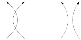
Figure 1: Direct self-tangency perestroika

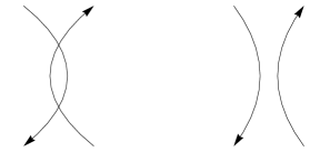
Figure 2: Inverse self-tangency perestroika

The move from Figure 3 corresponds to passing through a triple point. Such a move is called the triple point perestroika.

              

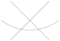
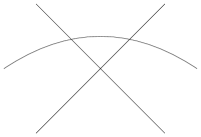
Figure 3: Triple point perestroika

Arnold [1] has shown that in the case $X={\mathbb{R}}^{2}$ there are three degree 1 (in Vassiliev’s sense) invariants corresponding to these moves. We do not specify the orientations at Figure 3 as all such choices combine to a single degree 1 invariant.

The invariant corresponding to the direct self-tangency perestroika is called $J_{+}$. It increases by 2 if such a move is performed in the direction when the number of nodes is increased by 2 and remains invariant if we perform either an inverse self-tangency or a triple point perestroika. (If we perform the direct self-tangency move in the opposite direction, then $J_{+}$ decreases by 2 accordingly.)

Similarly, $J_{-}$ is increased by 2 if an inverse self-tangency perestroika is performed in the direction when the number of nodes is decreased by 2 and remains invariant if we perform a direct self-tangency or a triple point perestroika.

Furthermore, there is a consistent choice of direction for performing the triple point perestroika. This choice allows us to declare that the third invariant (called the strangeness $St$) increases by 1 when the triple point perestroika is performed in this direction and does not change when any of the self-tangency perestroikas is performed. The rule for specifying this direction is indeed quite strange, although it was clarified by Shumakovich in [16] with the help of an explicit formula.

It was shown in [1] that if we start from a generic immersion, perform a number of the moves discussed above and return to the same generic immersion, then the total increment for each of the numbers $J_{+}$, $J_{-}$ and $St$ is zero. Thus, to turn $J_{+}$, $J_{-}$ and $St$ to conventional integer-valued invariants it is sufficient to choose their normalization on one generic immersion for each possible $\operatorname{rot}(K)$. This was done in [1] (in such a way that the resulting invariants are additive with respect to the connected sum).

From the definition, $J_{+}-J_{-}$ equals to the number of nodes of the generic immersion. It was noted by Viro [23] that $J_{-}$ can be easily computed from the complex orientation formula. In the same paper, Viro gave a well-defined adaptation of $J_{-}$ for immersed curves in $\mathbb{RP}^{2}$, the situation we consider in this paper.

2.2 Back to smooth ovals: smoothing of an immersion

Let $K\subset\mathbb{RP}^{2}$ be an immersion to $\mathbb{RP}^{2}$ of a disjoint union of a collection of oriented circles. By Example 2.4 we have $\operatorname{rot}(K)\in{\mathbb{Z}}_{4}$ (if $K$ is multicomponent, then its rotation number is the sum of the rotation numbers of the components of $K$), while the parity of $\operatorname{rot}(K)$ is determined by the parity of the homological class $[K]\in H_{1}(\mathbb{RP}^{2};{\mathbb{Z}})={\mathbb{Z}}_{2}$ which we call the degree $d=d(K)$ of $K$.

Assume that the immersed curve $K$ is generic (as before, it means that all self-crossing points are nodes). Let $n=n(K)$ be the number of nodes of $K$, and let $K_{\circ}\subset\mathbb{RP}^{2}$ be the collection of smoothly embedded oriented circles (defined up to isotopy) obtained from $K$ by smoothing every node of $K$ as shown on Figure 4. Note that to each node $p\in K$ we associate a closed embedded path $I_{p}\subset\mathbb{RP}^{2}$ with two endpoints on the corresponding two arcs of the smoothing and not intersecting $K_{\circ}$ at inner points of the path.

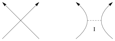
Figure 4: Smoothing according to the orientation and appearance of the vanishing cycle $I$

Definition 2.6.

The oriented curve $K_{\circ}$ is called smoothing of $K$. The intervals $I_{p}$ are called vanishing cycles corresponding to nodes $p$. The diagram

$$\Delta_{K}=(K_{\circ};\bigcup\limits_{p}I_{p}),$$ (1)

where $p$ runs over all nodes of $K$, is called the smoothing diagram of $K$.

Note that all vanishing cycles $I_{p}$ in the diagram $\Delta_{K}$ are disjoint.

Definition 2.7.

Let $L\subset\mathbb{RP}^{2}$ be a collection of disjoint oriented embedded circles. An $L$-membrane $I_{p}\subset\mathbb{RP}^{2}$ is a smoothly embedded interval such that $I_{p}\cap L$ coincides with the two endpoints of $I_{p}$ and at these endpoints the interval $I_{p}$ is transverse to $L$.

We say that an $L$-membrane $I_{p}$ is coherent (with respect to the orientation on $K_{\circ}$) if there exists a deformation of $I_{p}$ in the class of $L$-membranes disjoint from $I_{p}$ so that the endpoints move according to the orientations. In other words, $I_{p}$ is coherent if the orientations of $L$ are as shown on Figure 4.

An (abstract) smoothing diagram $\Delta=(L;I)$ consists of a collection $L\subset\mathbb{RP}^{2}$ of disjoint oriented embedded circles and a collection $I=\bigcup_{p}I_{p}$ of disjoint embedded closed intervals $I_{p}\subset\mathbb{RP}^{2}$ so that the number of intervals $I_{p}$ is finite and each interval $I_{p}$ is a coherent $L$-membrane. We consider such diagrams $(L;I)$ and $(L^{\prime};I^{\prime})$ equivalent if they are isotopic (meaning the existence of an isotopy identifying $L$ and $L^{\prime}$ as well as $I$ and $I^{\prime}$).

Proposition 2.8.

For every smoothing diagram $\Delta$ there exists a generic immersion $K$ of a disjoint union of oriented circles to $\mathbb{RP}^{2}$ such that $\Delta=\Delta_{K}$. Moreover, $K$ is unique up to isotopy.

The proof of this proposition is straightforward. We collapse every coherent membrane by performing the move opposite to the smoothing depicted at Figure 4.

Let $K\subset\mathbb{RP}^{2}$ be a generic immersion of a disjoint union of oriented circles. We have a well defined lift $\tilde{K_{\circ}}\in T_{1}(\mathbb{RP}^{2})$ as well as its homology class $\operatorname{rot}(K_{\circ})=[\tilde{K}_{\circ}]\in H_{1}(T_{1}(\mathbb{RP}^{2}))$. Denote with $l(K)$ the number of connected components of $K_{\circ}$ and with $k$ the number of circles in the immersion $K$ (i.e., the number of connected components of $\tilde{K}$).

Lemma 2.9.

We have

$$\operatorname{rot}(K_{\circ})=\operatorname{rot}(K).$$

Furthermore,

$$l(K)\leq n(K)+k,$$

$$l(K)=n(K)+k\mod 2.$$

Proof.

The homology class in $H_{1}(T_{1}(\mathbb{RP}^{2})$ is preserved under each smoothing. Let us consecutively smooth nodes as in Figure 4, one by one. At each step we increase or decrease the number of components of $\tilde{K}$ by 1, depending on whether the two branches of the node belong to the same or distinct components. ∎

The following statement can be viewed as the $\mathbb{RP}^{2}$-version of the Whitney formula [24]. It determines $\operatorname{rot}(K)$ once we know the degree of $K$ and $n(K)$.

Lemma 2.10.

If the degree $d(K)$ of $K\subset\mathbb{RP}^{2}$ is even, then

$$\operatorname{rot}(K)=2n(K)+2k\in{\mathbb{Z}}_{4}.$$

If $d(K)$ is odd, then

$$\operatorname{rot}(K)=2n(K)+2k-1\in{\mathbb{Z}}_{4}.$$

Proof.

When smoothing, at each step we change the parity of the number of components of $\tilde{K}$ by 1, but preserve its homology class $[\tilde{K}]=\operatorname{rot}(K)$. Once all nodes are smoothed we have $a$ even degree components and $b$ odd degree components. Each such even degree component is isotopic to a small circle and thus its rotation number is 2. Each odd degree component is isotopic to a line and thus its rotation number is 1.

We have $a+b=n(K)+k\mod 2$, $b=d(K)\mod 2$, and $b\leq 1$, while $\operatorname{rot}(K)=2a+b\mod 4$ which implies the statement of the lemma. ∎

Theorem 2.5 implies the following statement.

Corollary 2.11.

Two generic immersions of a circle to $\mathbb{RP}^{2}$ with the same parity of the number $n$ of nodes and the same degree $d$ are homotopic in the class of immersions.

Let $K\subset\mathbb{RP}^{2}$ be a generic immersion of a disjoint union of oriented circles, and let $p\in\mathbb{RP}^{2}\setminus K$ be a point. We choose an isomorphism between the group $H_{1}(\mathbb{RP}^{2}\setminus\{p\};{\mathbb{Z}})$ and $\frac{1}{2}{\mathbb{Z}}$. The only ambiguity in the choice of this isomorphism is the sign. The index $\pm\operatorname{ind}_{K}(p)$ is the half-integer well-defined up to sign given by $[K]\in H_{1}(\mathbb{RP}^{2}\setminus\{p\};{\mathbb{Z}})$. Using half-integers guarantees that the index jumps by one each time we pass a branch of $K$. The absolute value $|\operatorname{ind}_{K}(p)|$ and the square $\operatorname{ind}^{2}_{K}(p)$ are well-defined half- resp. quarter-integer numbers. Hence $|\operatorname{ind}_{K}|$ and $\operatorname{ind}^{2}_{K}$ are locally constant functions on $\mathbb{RP}^{2}\setminus K$.

Given a small neighbourhood $U$ of a node $p$ of $K$, the set $U\setminus K$ consists of four connected components, called quadrants here. When smoothing $K$ to $K_{\circ}$, the two opposite quadrants which stay disconnected are called stable, the other two quadrants which get connected are called unstable. A locally constant function $f:\mathbb{RP}^{2}\setminus K\to{\mathbb{R}}$ which at each node $p$ of $K$ takes the same value on the two unstable quadrants is called smoothable. The functions $|\operatorname{ind}_{K}|$ and $\operatorname{ind}^{2}_{K}$ are of this form. Obviously, in this case $f$ descends to a unique function $f_{\circ}:\mathbb{RP}^{2}\setminus K_{\circ}\to{\mathbb{R}}$ (see Figure 5).

Figure 5: (Un-)stable quadrants and a smoothable function $f$

Let $f:\mathbb{RP}^{2}\setminus K\to{\mathbb{R}}$ be a locally constant function. We extend $f$ to the whole plane $\mathbb{RP}^{2}$ as follows. Suppose that $p\in K$. If $p$ is not one of the nodes of $K$, we define $f(p)$ as the average of the values of $f$ at the two regions of $\mathbb{RP}^{2}\setminus K$ adjacent to $p$. If $p\in K$ is a node, we define $f(p)$ to be the average of the values of $f$ on the two stable quadrants (see Figure 6). Note that when we apply this construction to $|\operatorname{ind}_{K}|$ and $\operatorname{ind}^{2}_{K}$, in general we get $(|\operatorname{ind}_{K}|(p))^{2}\neq\operatorname{ind}^{2}_{K}(p)$ for $p\in K$.

Figure 6: Extension of a function $f$ to $\mathbb{RP}^{2}$

Following [21] we define the integral $\int\limits_{\mathbb{RP}^{2}}fd\chi$ with respect to Euler characteristic for any function $f:\mathbb{RP}^{2}\to{\mathbb{R}}$ with the finite image $f(\mathbb{RP}^{2})\subset{\mathbb{R}}$ and such that there exists a cellular decomposition of $\mathbb{RP}^{2}$, where the inverse image $f^{-1}(j)$ is a finite union of open cells for any $j\in{\mathbb{R}}$. Namely, if a set $A\subset\mathbb{RP}^{2}$ is a finite union of open cells, we set $\chi(A)\in{\mathbb{Z}}$ to be the difference of the number of even-dimensional cells in $A$ with the number of odd-dimensional cells in $A$. This is nothing else but the Euler characteristic of $A$, but if we are to compute it homologically, we have to take homology with closed support. E.g. for a single $n$-dimensional cell $A\approx{\mathbb{R}}^{n}$ we have $\chi(A)=(-1)^{n}$.

Definition 2.12 (Viro, [21]).

We define

$$\int_{\mathbb{RP}^{2}}fd\chi=\sum\limits_{j\in f(\mathbb{RP}^{2})}j\cdot\chi(f^{-1}(j))=\sum\limits_{\sigma\text{ cell}}(-1)^{\dim(\sigma)}f(\sigma).$$

The latter sum is taken over the open cells $\sigma$ such that $f|_{\sigma}$ is constant.

Proposition 2.13.

For any smoothable locally constant function $f:\mathbb{RP}^{2}\setminus K\to{\mathbb{R}}$ we have

$$\int\limits_{\mathbb{RP}^{2}}fd\chi=\int\limits_{\mathbb{RP}^{2}}f_{\circ}d\chi,$$

where the integrals are considered for the extensions of $f$ and $f_{\circ}$ to $\mathbb{RP}^{2}$.

Proof.

We may choose the cellular decompositions of $\mathbb{RP}^{2}$ for $f$ and $f_{\circ}$ so that one decomposition can be obtained from the other by replacing each node $p$ of $K$ with the vanishing cycle $I_{p}$ subdivided into three cells: the two endpoints and the relative interior. The contribution of $I_{p}$ to $\int\limits_{\mathbb{RP}^{2}}f_{\circ}d\chi$ coincides with the contribution of $p$ to $\int\limits_{\mathbb{RP}^{2}}fd\chi$. ∎

The invariants $J_{\pm}$ and $\operatorname{St}$ from [1] also have counterparts for immersions to $\mathbb{RP}^{2}$.

Definition 2.14 (Viro, [23]).

Let $K\subset\mathbb{RP}^{2}$ be a generic immersion of an oriented circle. Put

$$J_{-}(K)=1-\int\limits_{\mathbb{RP}^{2}}\operatorname{ind}^{2}_{K}d\chi.$$

Furthermore, in [23] it was shown that the number $J_{-}(K)$ defined in this way does not change under the direct double tangency perestroika or under the triple point perestroika. It decreases by 2 under the inverse self-tangency perestroika when the number of nodes is increased.

As in the case of immersions in ${\mathbb{R}}^{2}$ we can use the equality $J_{+}(K)-J_{-}(K)=n(K)$ as the definition of $J_{+}(K)$. In our context it is more convenient to use the integral $\int\limits_{\mathbb{RP}^{2}}\operatorname{ind}^{2}_{K}d\chi$ itself as the invariant of an immersion instead of either $J_{+}(K)$ or $J_{-}(K)$. We set up the following definition accordingly.

Definition 2.15.

The complex orientation invariant of $K$ is the number

$$\operatorname{Or}(K)=\int\limits_{\mathbb{RP}^{2}}\operatorname{ind}^{2}_{K}d\chi.$$

Figure 7: An example for $\operatorname{Or}(K)=2-\frac{1}{2}-\frac{5}{2}+1+4=4$ and $\operatorname{St}(K)=-1+\frac{5}{2}-\frac{1}{2}=1$.

An example of this invariant is given in Figure 7. Note that this invariant makes sense not only for generic immersions of single circle, but also for generic immersions of disjoint collections of circles. In particular, it makes sense for $K_{\circ}$ (an embedded collection of circles obtained from $K$).

Corollary 2.16.

We have $\operatorname{Or}(K_{\circ})=\operatorname{Or}(K)$.

Proof.

The corollary follows from Proposition 2.13 since $\operatorname{ind}^{2}_{K_{\circ}}=(\operatorname{ind}^{2}_{K})_{\circ}$. ∎

For the rest of this subsection we assume that $K\subset\mathbb{RP}^{2}$ is an immersion of a single circle. Following [23] we introduce the strangeness invariant for generic immersions in $\mathbb{RP}^{2}$ with the help of the Shumakovich’ formula [16]. Let us choose a base point $q\in K$ that is not a node of $K$. Each node $p\in K$ now gets a canonical local orientation since we have the order on the oriented branches of $K$ as they can be traced from $q$ following the orientation of $K$. This local orientation can be used to fix the sign of $\operatorname{ind}_{K,q}(p)$. Namely, we set $+1$ to represent the class of a small oriented circle around $p$ in $H_{1}(\mathbb{RP}^{2}\setminus\{p\};{\mathbb{Z}})$.

Definition 2.17 (Shumakovich-Viro, [16]).

We set

$$\operatorname{St}(K)=-\sum\limits_{p}\operatorname{ind}_{K,q}(p)+\operatorname{ind}^{2}_{K}(q)-\frac{1}{2},$$

where the sum is taken over all nodes $p\in K$.

The number $\operatorname{St}(K)$ does not depend on the choice of the base point $q\in K$ and stays invariant under both direct and inverse self-tangency perestroikas. It changes by $\pm 1$ under the triple point perestroika and thus provides the counterpart of Arnold’s strangeness for generic immersions of a circle into the projective plane (see Figure 7).

The relative interior of a $K_{\circ}$-membrane $I_{p}$ is contained in a single component of $\mathbb{RP}^{2}\setminus K_{\circ}$. Thus $|\operatorname{ind}_{K_{\circ}}(I_{p})|$ is well-defined. Definition 2.17 may be rewritten as follows in terms of the smoothing diagram $\Delta_{K}$:

$$\operatorname{St}(K)=\operatorname{St}(\Delta_{K})=\sum\limits_{p}\sigma_{q}(I_{p})|\operatorname{ind}_{K_{\circ}}(I_{p})|+\operatorname{ind}^{2}_{K}(q)-\frac{1}{2}.$$ (2)

Here the base point $q$ can be placed anywhere on $K_{\circ}$ outside of the endpoints of the vanishing cycles. To define the signs $\sigma_{q}(I_{p})=\pm 1$ we trace the diagram $\Delta_{K}$ starting from $q$ according to the orientation of $K_{\circ}$ and jump to the other branch of $K_{0}$ at every vanishing cycle $I_{p}$. Note that whenever $|\operatorname{ind}_{K_{\circ}}(I_{p})|\neq 0$ there is a canonical orientation of $I_{p}$ from the arc of $K_{\circ}$ with a smaller $|\operatorname{ind}_{K_{\circ}}|$ to the arc with the larger $|\operatorname{ind}_{K_{\circ}}|$. If the first jump at $I_{p}$ is in the direction of this orientation, then we set $\sigma_{q}(I_{p})=1$, otherwise $\sigma_{q}(I_{p})=-1$. Figure 8 shows why this sign choice agrees with the previous one. On the left hand side, we depicted the local behaviour of $\operatorname{ind}_{K,q}$ around a node $p$. Here, the choice of first and second branch induces the local orientation to be counterclockwise, and this implies that $\operatorname{ind}_{K,q}$ decreases by 1 when we cross a branch from left to right. On the right hand side we depicted the two jumps between the branches of the local smoothing, together with the values of $|\operatorname{ind}_{K_{\circ}}|$. We want to compare the signs of $i=\operatorname{ind}_{K,q}(p)$ and $\sigma_{q}(I_{p})$. Assume $i>0$, then $|i+1|>|i-1|$, and the first jump is from greater to lower value of $|\operatorname{ind}_{K_{\circ}}|$, hence $\sigma_{q}(I_{p})=-1$. It follows $\text{sgn}(i)=-\sigma_{q}(I_{p})$, which shows that definition 2.17 and formula (2) are consistent.

Figure 8: The consistency of the two sign rules, namely $\text{sgn}(i)=-\sigma_{q}(I_{p})$

2.3 The immersion graph $\Gamma(K)$

To classify generic immersions of a disjoint union of circles with a given number of nodes we can list their smoothing diagrams (see Proposition 2.8). In turn, to exhaust such diagrams it is useful to extract a certain graph from the smoothing diagram and study the properties of this graph.

Let $K\subset\mathbb{RP}^{2}$ be a generic immersion of a disjoint union of $k$ oriented circles. We form a graph $\Gamma(K)$ whose vertices are the connected components of $K_{\circ}$ and edges are the vanishing cycles of $\Delta_{K}$.

Lemma 2.18.

If $l(K)=n(K)+k$, then the graph $\Gamma(K)$ is a disjoint union of $k$ trees. If $k=1$, then $\Gamma(K)$ is connected and $b_{1}(\Gamma(K))=n(K)+1-l(K)=0\mod 2$.

As usual, we denote with $b_{1}(\Gamma)$ the first Betti number of a graph $\Gamma$, i.e., the number of independent cycles of $\Gamma$.

Proof.

If $l(K)=n(K)+k$, then each vanishing cycle decreases the number of connected components of the smoothing diagram exactly by one. This implies the first statement of the lemma. If $K$ is connected, the graph $\Gamma(K)$ is also connected. The modulo 2 congruence is provided by Lemma 2.9. ∎

Definition 2.19.

The immersion graph of a generic immersion $K\subset\mathbb{RP}^{2}$ is the graph $\Gamma(K)$ enhanced with the following extra information (so that the smoothing diagram $\Delta_{K}$ can be uniquely recovered from the enhanced graph $\Gamma(K)$). The enhancement of $\Gamma(K)$ consists of

• (1. oriented edges.) the orientation for some of the edges of $\Gamma(K)$,

• (2. ribbon structure.) the ribbon structure for $\Gamma(K)$,

• (3. two-coloring.) a two-coloring of its vertices and

• (4. projective enhancement.) a projective enhancement of $\Gamma(K)$ described below (the treatment is different depending on $d(K)$).

We describe these enhancements in details one by one.

1. Oriented edges. Each edge $E$ of $\Gamma(K)$ connects two components of $K_{\circ}$. If these components are ovals with disjoint interiors then we do not orient $E$. Also we do not orient $E$ if it is a loop-edge, i.e., corresponds to a vanishing cycle connecting an oval to itself.

If the two components are nested ovals, i.e., the interior of one oval contains the other oval, then we orient the edge in the direction from the interior oval to the exterior one.

Recall that all connected components of $K_{\circ}$ except possibly for a single one (which appears if $d(K)\neq 0$) are ovals. If an edge $E\subset\Gamma(K)$ connects an oval to the pseudoline, then we orient $E$ in the direction from the oval to the pseudoline. Note that no vanishing cycle may connect a pseudoline in $\mathbb{RP}^{2}$ to itself by the orientation reasoning.

2. Ribbon structure. As there is some ambiguity in what people call ribbon graphs we start by quoting one of the most commonly accepted definitions of an ribbon graph. It is a finite graph $\Gamma$ with a choice of cyclic order of adjacent half-edges for every vertex $v\in\Gamma$.

Recall that given such a structure on $\Gamma$ we may canonically reconstruct the oriented surface $S_{\Gamma}$ containing the graph $\Gamma$ as its deformational retract as follows. We take a copy of the closed oriented disk $D_{v}$ for each vertex $v\in\Gamma$ of valence $\operatorname{val}(v)$. Then we mark $\operatorname{val}(v)$ points at the boundary $\partial D_{v}$ so that the boundary orientation agrees with the cyclic order from the ribbon structure. Finally, we attach an orientation-preserving ribbon $R_{E}$ connecting the disks $D_{v}$ and $D_{v^{\prime}}$ at the corresponding marked points for each edge $E$ connecting $v$ and $v^{\prime}$.

Recall that our immersion $K$ is oriented and so are all components of $K_{\circ}$. Because of this, the graph $\Gamma(K)$ admits a canonical ribbon structure coming from the cyclic order of vanishing cycles adjacent to a connected component $C_{v}\subset K_{\circ}$ associated to a vertex $v\in\Gamma(K)$.

Nevertheless, the surface $S_{\Gamma}$ (that is conventionally associated to a ribbon graph as we reviewed above) does not have a direct relation to the topology of $K_{\circ}\subset\mathbb{RP}^{2}$. Instead, our goal is to use additional structure that we define on $\Gamma(K)$ so that we may recover the pair $(\mathbb{RP}^{2};\Delta(K))$. We describe this procedure in the next subsection, once we define the remaining part of the enhancement for $\Gamma(K)$.

3. Two-coloring.

The vertices of $\Gamma$ are colored by two colors in the following way. An oriented pseudoline $J\subset\mathbb{RP}^{2}$ defines the orientation of $\mathbb{RP}^{2}\setminus J$. An oriented oval disjoint from $J$ is positive (respectively, negative) if it defines in its interior the orientation opposite to (respectively, the orientation coinciding with) the one given by the orientation of $\mathbb{RP}^{2}\setminus J$. If $d(K)$ is odd we choose $J=C_{u}$, the pseudoline component of $K_{\circ}$. If $d(K)$ is even, we fix some pseudoline $J\subseteq\mathbb{RP}^{2}\setminus K_{\circ}$. We then set the vertices corresponding to all positive ovals to be white vertices, all other vertices (corresponding to negative ovals or the pseudoline) are blue vertices. If $d(K)$ is even, due to the choice of $J$ the colors are only well-defined up the following flip. We say a vertex $v$ dominates a vertex $v^{\prime}$ if they can be connected via an oriented edge leading to $v$. Let $v$ be maximal with respect to this partial order (i.e., $v$ corresponds to an exterior oval). Then the colors are well-defined up to flipping the colors of $v$ and all the vertices dominated by $v$ simultaneously. The colors are a convenient way to describe the following property of $\Gamma(K)$. For every cycle in $\Gamma(K)$, the number of non-oriented edges not contained in the root cluster is even.

Before we describe the projective enhancement, let us collect some properties of the first three enhancements satisfied by immersion graphs $\Gamma=\Gamma(K)$.

Definition 2.20.

A cluster of vertices is a maximal connected subgraph $\Gamma^{\prime}\subset\Gamma$ such that all its edges are unoriented (i.e., any other connected subgraph without oriented edges is either contained in $\Gamma^{\prime}$ or disjoint from it).

Proposition 2.21 (Oriented edges).

If $\Gamma=\Gamma(K)$ is the immersion graph of a generic immersion $K\subset\mathbb{RP}^{2}$, then all oriented outgoing edges from a cluster of vertices $A\subset\Gamma(K)$ lead to the same vertex $v\in\Gamma(K)$.

There is a unique cluster $U$ of vertices of $\Gamma(K)$ such that there are no outgoing edges from $U$. In the case $d(K)\neq 0$ this cluster consists of the vertex associated to the pseudoline component of $K_{\circ}$.

Proof.

An oval $C_{v}\subset K_{\circ}$ might be contained inside several other ovals of $K_{v}$, but all of them are nested. A vanishing cycle may connect $C_{v}$ only with the innermost oval from this collection. The second statement follows from the fact that $K$ and therefore $\Gamma$ are connected. ∎

If all outgoing edges from a cluster of vertices $A\subset\Gamma(K)$ lead to a vertex $v\in\Gamma(K)$, we say that the cluster $A$ is dominated by $v$. The unique cluster $U$ of $\Gamma(K)$ such that there are no outgoing edges from $U$ is called the root cluster of $\Gamma(K)$.

Proposition 2.22.

Let $E$ be an edge connecting vertices $v,v^{\prime}\in\Gamma$. If $E$ is oriented, then $v$ and $v^{\prime}$ are of the same color. If $E$ is non-oriented and not contained in the root cluster, then $v$ and $v^{\prime}$ are of different color.

Proof.

Let $J$ denote the pseudoline used to define the colors. In both cases of the statement, we may assume that the vanishing cycle $I$ corresponding to $E$ does not intersect $J$. The statement than follows from the coherence of $I$ (see 2.7). ∎

For a vertex $v$, we denote with $\operatorname{Ad}(v)$ the set of all edges adjacent to $v$. The sets $\operatorname{Ad}^{+}(v)$ and $\operatorname{Ad}^{-}(v)$ are the subsets of $\operatorname{Ad}(v)$ formed by the edges oriented away from $v$ and towards $v$, respectively.

Let $A$ be a cluster of vertices. Build a surface $\Sigma_{A}$ as follows. Take a disjoint union $\Delta$ of oriented discs $D_{v}$ over all $v\in A$. For each vertex $v\in A$, mark points, indexed by $\operatorname{Ad}(v)\setminus\operatorname{Ad}^{-}(v)$, on $\partial D_{v}$ in the cyclic order provide by the ribbon structure of $A$. For each edge connecting $v,v^{\prime}\in A$ we add a ribbon to $\Delta$ connecting small neighborhoods of the corresponding marked points at $\partial\Delta$ so that the ribbon disrespects the orientations of $D_{v}$ and $D_{v^{\prime}}$. Denote the resulting surface with $\Sigma_{A}$.

Proposition 2.23.

Suppose that $\Gamma=\Gamma(K)$ is an immersion graph. Let $A$ be a cluster which is not the root cluster. Then the surface $\Sigma_{A}$ is homeomorphic to a sphere with holes. Moreover, all the remaining marked points (indexed by $\bigcup_{v}\operatorname{Ad}^{+}(v)$) lie on the same boundary component of $\Sigma_{A}$.

The latter component is called the exterior boundary component.

Proof.

The surface $\Sigma_{A}$ is homeomorphic to a regular neighborhood $N$ of the part of the smoothing diagram formed by the ovals and vanishing cycles from $A$. All remaining marks sit on the exterior boundary component of $N$ (the boundary of the non-oriented component in $\mathbb{RP}^{2}\setminus N$). ∎

Remark 2.24.

The previous proposition can also be expressed more combinatorially. Let $A$ be a cluster of $\Gamma$ which is not the root cluster. A ribbon cycle in $A$ is an oriented closed path $p$ in $A$ such at each white (resp. blue) vertex $v$ the outgoing edge is the successor (resp. predecessor) of the incoming edge (according to the cyclic order given by the ribbon structure). The oriented edges $e\in\operatorname{Ad}^{+}(v)$ lying between the incoming and outgoing edge are said to lie on $p$. Let $V,E,B$ be the number of vertices of $A$, edges of $A$, ribbon cycles of $A$, respectively. Then the proposition can be reformulated as

$$V-E+B=2$$

and the condition that all edges in $\bigcup_{v\in A}\operatorname{Ad}^{+}(v)$ lie on the same ribbon cycle.

Let us finally discuss the fourth enhancement.

4. Projective enhancement.

If $d(K)=0$, consider the surface $\Sigma_{A}$, where $A$ is the root cluster. If $\Sigma_{A}$ is oriented, the projective enhancement is a choice of boundary component of $\Sigma_{A}$, namely the exterior one (see the proof of Proposition 2.23). If $\Sigma_{A}$ is non-oriented, no extra information is needed.

If $d(K)=1$, i.e., $[K]\neq 0\in H_{1}(\mathbb{RP}^{2})$, there is a pseudoline component of $K_{\circ}$. We treat the corresponding vertex $u\in\Gamma(K)$ as the root vertex. In figures, we draw the root vertex in a special way, as a horizontal line.

As any other vertex of $\Gamma(K)$ the vertex $u$ comes with a natural cyclic order on the adjacent edges. This order is the cyclic order in which the vanishing cycles appear when we travel along the pseudoline $C_{u}\subset K_{\circ}$.

There is however an extra data we can extract from the way how the vanishing cycles are attached to $C_{u}$. Even though the component $C_{u}\subset\mathbb{RP}^{2}$ is one-sided, locally it has two sides and we can check whether the two consecutive vanishing cycles come to $C_{u}$ from the same side, or from opposite sides. In the latter case we place a cross on the corresponding arc of the circle corresponding to the vertex $u\in\Gamma(K)$. Since $C_{u}$ is one-sided, the total number of crosses on the circle corresponding to $u$ must be odd. This information is the projective enhancement in the case $d(K)=1$.

If $v\neq u$ is not a root vertex, we define the a cyclic order on $\operatorname{Ad}^{-}(v)$ induced by the cyclic order on $\operatorname{Ad}(v)$. For the root vertex $u$ we define the cyclic order on $\operatorname{Ad}^{-}(u)$ by requiring that the edge following $E\in\operatorname{Ad}^{-}(u)$ is the first edge after $E$ (in the order defined by the orientation of the pseudoline $C_{u}$) that is separated from $E$ by an even number of crosses.

Let $A$ be a cluster, and let $\operatorname{Ad}^{+}(A)=\bigcup_{v}\operatorname{Ad}^{+}(v)$ denote the edges adjacent to a cluster $A$ and oriented in the direction outgoing from $A$. (Note that $\operatorname{Ad}^{+}(U)=\emptyset$ for the root cluster $U$.) Due to Proposition 2.23, the orientation on the exterior boundary component of $\Sigma_{A}$ induces a cyclic order on $\operatorname{Ad}^{+}(A)$.

Proposition 2.25.

Let $\Gamma=\Gamma(K)$ be an immersion graph. For any cluster $A\subset\Gamma$ dominated by a vertex $w$ the cyclic order on $\operatorname{Ad}^{+}(A)\subset\operatorname{Ad}^{-}(w)$ agrees with that on $\operatorname{Ad}^{-}(w)$. Furthermore, the sets $\operatorname{Ad}^{+}(A)$ for different clusters dominated by $w$ are unlinked, i.e., if $A$ and $B$ are two clusters dominated by $w$, there is a segment in $\operatorname{Ad}^{-}(w)$ (according to the cyclic order) that contains $\operatorname{Ad}^{+}(A)$ and is disjoint from $\operatorname{Ad}^{+}(B)$.

Proof.

The proposition follows since every component of $\mathbb{RP}^{2}\setminus K_{\circ}$ adjacent to $w$ and $A$ is homeomorphic to an open disk with punctures. ∎

Definition 2.26.

A graph $\Gamma$ enhanced with the a partial orientation of its edges, a ribbon structure, a two-coloring and a projective enhancement as defined in paragraphs 1. – 4. above and satisfying the properties of propositions 2.21, 2.22, 2.23 and 2.25 is called an enhanced graph.

We conclude these considerations with the following elementary statement.

Proposition 2.27.

Let $\Gamma$ be an enhanced graph for odd $d$. Then there exists a generic immersion $K\subset\mathbb{RP}^{2}$ of a collection of disjoint oriented circles with $\Gamma=\Gamma(K)$. The isotopy type of $K$ is determined by $\Gamma$.

Proof.

We construct the smoothing diagram in $\mathbb{RP}^{2}$ by representing the root vertex $u$ with a pseudoline and the other vertices with ovals. Propositions 2.21, 2.25 and 2.23 ensure existence of such diagram while Proposition 2.22 ensures that the orientations are compatible. Then we “unsmooth” $K_{\circ}$, i.e., replace each vanishing cycle with a node as in Figure 4. Topological uniqueness is inductive. ∎

Remark 2.28.

In the case $d=0$, only few changes are necessary. Proposition 2.27 still holds if we add the requirement that the surface $\Sigma_{A}$ for the root cluster $A$ is homeomorphic to either a sphere with holes or $\mathbb{RP}^{2}$ with holes. (In terms of 2.24, we want $V-E+B=1$ or $2$.) Then this surface can be embedded in $\mathbb{RP}^{2}$ by gluing discs to all boundary components, except possibly to the boundary component specified by the projective enhancement, to which we glue a Möbius strip instead. The construction then continues as in the odd case.

Remark 2.29.

Figures 10, 10, 12, 12 show the Reidemeister moves in terms of the graph $\Gamma(K)$. Here and in the following, the edges in the root cluster connecting vertices of the same color are marked with the symbol $\infty$ (which expresses that the corresponding vanishing cycles intersect the pseudoline $J$ “at infinity” which we chose in order to define the colors).

                

                

          

       

                 

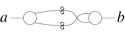
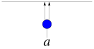
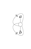
Figure 9: Direct self-tangency perestroika for $\Gamma(K)$

                 

                 

                   

                   

                  

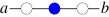
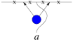
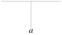
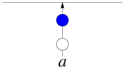
Figure 10: Inverse self-tangency perestroikas for $\Gamma(K)$

         

         

         

         

         

         

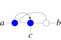
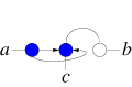
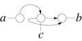
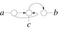
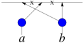
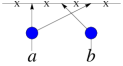
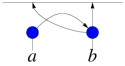
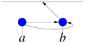
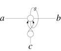
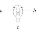
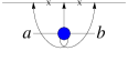
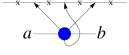
Figure 11: Weak triple point perestroikas $\Gamma(K)$

     

     

     

     

     

     

     

     

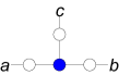
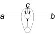
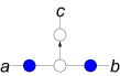
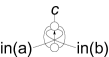
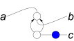
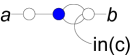
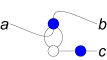
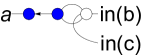
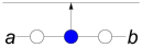
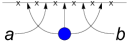
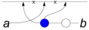
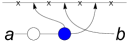
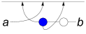
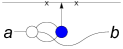
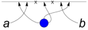
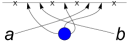
Figure 12: Strong triple point perestroikas $\Gamma(K)$

The following conventions are adopted. Each letter $a$, $b$, $c$ stands for a sequence of edges (one after another in the cyclic order of the ribbon graph) adjacent to a vertex of $\Gamma(K)$. These edges may be oriented or unoriented. The symbol $"in(a)"$ stands for the inversion of the sequence $a$, i.e., inserting it in the reverse order. Such an inversion happens every time the sequence gets attached to a vertex of different color after the move.

Also, some moves in Figure 12 change a sequence ($a$ or $b$) from being adjacent to a non-root vertex (depicted by a blue or white disk) to the root vertex (depicted by the line). Recall that all edges adjacent to the root vertex are oriented towards it. If an edge in a sequence $a$ (or $b$) adjacent to a non-root vertex was unoriented, then it becomes oriented after such a move. If it was already oriented, then it remains oriented, but we add two crosses, one on each side of its adjacency to the line. Recall that this means that the corresponding vanishing cycle is attached from the other (local) side of the non-contractible component of the smoothing diagram.

The third and the fifth move in Figure 10, as well as the fifth move in Figure 12, involve ovals of the same color connected with non-oriented edges. These moves are only applicable to the even $d$ case as the relative interior of the corresponding vanishing cycles must intersect the auxiliary pseudoline $J\subset\mathbb{RP}^{2}$ while being disjoint from $K_{\circ}$.

2.4 Classification of generic immersions of a circle with small $n$

If $n(K)=0$, then our immersion is an embedding. If $d(K)=1\mod 2$, then the embedding is isotopic to the standard embedding $\mathbb{RP}^{1}\subset\mathbb{RP}^{2}$. If $d(K)=0\mod 2$, then $K$ must be the standard embedding of a circle into $\mathbb{RP}^{2}$ as an oval (the one that bounds an embedded disk).

Immersion graphs provide an exhausting way to classify all immersions of a circle with a given number $n$ of nodes. To do that we may list all connected graphs which have $n$ edges and $m$ vertices with $m=n+1\mod 2$ enhanced as in Definition 2.19 and extract those that correspond to immersions of a circle.

If $n=1$, then the graph $\Gamma(K)$ must have two vertices (as the number of vertices is not greater than two and has the same parity). For $d=1\mod 2$ there is a unique graph $\Gamma(K)$, see Figure 15. For $d=0\mod 2$ there are two cases, see Figure 15 for the graphs and corresponding immersions.

In the case $n=2$, $d=1$ the graph $\Gamma(K)$ must have three vertices (as the root vertex can not be adjacent to itself if $\Gamma$ comes from an immersion to $\mathbb{RP}^{2}$). There are three possibilities depicted (along with the corresponding immersions) at Figure 15.

  

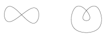
Figure 13: The graph and the corresponding immersion for $n=1$, $d=1$

Figure 14: Graphs and corresponding immersions for $n=1$, $d=0$

     

     

     

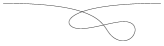
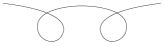
Figure 15: Graphs and corresponding immersions for $n=2$, $d=1$

As the final example of complete classifications of all generic immersions based on graphs $\Gamma(K)$ we consider the case $n=2$, $d=0$. In this case $\Gamma(K)$ may have three vertices or a single vertex. The classification is depicted on Figure 16 together with the smoothing diagrams themselves. Note that in the case of a single vertex, there are a priori two choices for the cyclic order at this vertex, but only the one shown in Figure 16 satisfies to 2.28. For the second choice, $\Sigma_{A}$ is a Klein bottle with holes ($V-E+B=1-2+1=0$, cf. 2.24).

                       

                     

                   

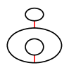
Figure 16: Graphs, diagrams and corresponding immersions for $n=2$, $d=0$

For higher $n$ the classification of generic immersions gets rather complicated fast (cf. [1]). However, there is a class of relatively simple immersions for arbitrary $n$ which we would like to distinguish.

Definition 2.30.

A generic immersion $K\subset\mathbb{RP}^{2}$ of a circle is called arboreal if the corresponding graph $\Gamma(K)$ is a tree.

Proposition 2.31.

If the degree $d$ is odd, then the arboreal immersions are in 1-1 correspondence with the ribbon rooted trees $T$ enhanced with the orientation of some of its edges towards the root as well as the data encoding the side change (denoted by crosses on the horizontal line in our pictures) for the edges adjacent to the root vertex of $T$. We require all edges adjacent to the root to be oriented.

If $d$ is even, then the arboreal immersions are in 1-1 correspondence with the ribbon (unrooted) trees $T$ enhanced with orientations of some of its edges in such a way that there exists at least one vertex to which all the orientations point out.

Proof.

If $d$ is odd, we start by the pseudoline representing the root and add the vanishing cycles adjacent to it according to the side data. To these cycles we attach the (even degree) immersions corresponding to the connected components of $T$ minus the union of its root and the open edges adjacent to the root.

If $d$ is even, the immersion $K$ may be deformed to ${\mathbb{R}}^{2}$ as $\Gamma(K)$ has no cycles. Take the subtree $T^{\prime}\subset T$ formed by the vertices on the headside of all oriented edges. The subtree $T^{\prime}$ also contains all edges between such vertices (which must be non-oriented). The subtree $T^{\prime}$ is represented by a collection of non-nested ovals in ${\mathbb{R}}^{2}$ and vanishing cycles between them. For each oriented edge adjacent to $T^{\prime}$ we take a vanishing cycle adjacent to the corresponding oval from its interior and proceed inductively. ∎

2.5 Classification of generic real rational curves of degree $4$

Here we illustrate how enhanced graphs and related smoothing diagrams can be used for classification of real nodal rational quartic curves in $\mathbb{RP}^{2}$. In this degree the classification is already known (see e.g. [4] for its recently found description in terms of chord diagrams). Let us consider several ways in which this classification can be formulated.

Recall that for a nodal rational curve in $\mathbb{RP}^{2}$, we denote by $h$, $e$, and $c$ the numbers of hyperbolic, elliptic, and imaginary nodes of the curve (see Section 1.2).

Theorem 2.32 (see [4]).

There are $13$ isotopy types of nodal rational curves of degree $4$ in $\mathbb{RP}^{2}$. These isotopy types are listed in Table 7. (The table contains each isotopy type on the right together with its “chord diagram”, explained in Proposition 2.33 and Remark 2.34, on the left.)

$h=3$

$e>0,c=0$

$c=2,h=1$

$c=2,e=1$

Table 7: Nodal rational quartics

Proof.

Assume first that $C$ does not have imaginary nodes and that $K={\mathbb{R}}C\setminus E$ (where $E$ is the set of elliptic nodes of $C$) is not an arboreal immersion. Then, we have $n=3-e$ and $l=n-1=2-e$, so $e=0,1$ (as usual, $n$ is the number of edges of $\Gamma(K)$, while $l$ is the number of its vertices; these two numbers have opposite parity for an immersion of a circle).

If $e=1$, then the smoothing diagram $\Delta_{K}$ consists of a single oval with two vanishing cycles. The corresponding immersion is unique by our $n=2$ classification. If the elliptic node sits outside the oval of $\Delta_{K}$ we get a contradiction to the Bézout theorem by tracing a line through an elliptic and one of the two hyperbolic nodes of $C$.

If $e=0$, then the graph $\Gamma(K)$ (which we assumed to be non-arboreal) has two vertices and three edges. Suppose that there is no vanishing cycle intersecting the auxiliary pseudoline $J$. Then, the corresponding two ovals of $\Delta_{K}$ must be nested. Otherwise, the line $L$ connecting any two of the three hyperbolic nodes must intersect ${\mathbb{R}}C$ also somewhere else by topological reasons. We get a contradiction with the Bézout theorem as each node already contributes two to the intersection number of $L$ and $C$.

If there is a vanishing cycle intersecting $J$, then each such vanishing cycle must correspond to a loop of $\Gamma(K)$. Indeed, if the two ovals of $\Delta_{K}$ are nested, then only the exterior oval may be adjacent to a vanishing cycle intersecting $J$. The unnested components correspond to vertices of different color, so a vanishing cycle intersecting $J$ cannot connect them in a way coherent with the orientation.

If we have a single loop at a vertex $v\in\Gamma(K)$, then there are two edges $e_{1},e_{2}$ connecting $v$ to a vertex $v^{\prime}$. These are the only edges adjacent to $v^{\prime}$. Therefore, $e_{1}$ and $e_{2}$ must be separated from each other by the two endpoints of the loop edge, as otherwise $K$ would have several components after normalization. Once again this excludes the possibility that the two ovals of $\Delta_{K}$ are unnested. The unique nested configuration is listed in Table 7.

If there are two loops at a vertex $v\in\Gamma(K)$, then we have a single edge connecting $v$ to $v^{\prime}$. As in the $e=1$ case, the cyclic ordering of the loop edges at $v$ is unique by the $n=2$ classification. When inserting the edge connecting $v$ to $v^{\prime}$, there is again only one choice due to symmetries.

We are left to consider the case when $C$ has a pair of imaginary nodes. There is exactly one remaining node. If it is hyperbolic, then the corresponding vanishing cycle connects two ovals that can be either nested or unnested. If the real node is elliptic, then ${\mathbb{R}}C\setminus E$ is an oval. The elliptic node can be either inside or outside this oval. ∎

All thirteen topological types of $(\mathbb{RP}^{2},{\mathbb{R}}C)$ described above can be easily realized by quadratic (Cremona) transformations of conics as specified in the following statement.

Proposition 2.33.

The 13 types of Theorem 2.32 can be obtained from conics by the quadratic transformation

$$[x_{0}:x_{1}:x_{2}]\mapsto[x_{1}x_{2}:x_{0}x_{2}:x_{0}x_{1}].$$ (3)

For each type, we show a suitable arrangement of a conic and the coordinate axes next to the curve in Table 7.

The proof of this proposition is straightforward.

Remark 2.34 (D’Mello, Viro, see [4]).

Nodal rational quartics in $\mathbb{RP}^{2}$ correspond to topological chord diagrams, that is, topological types of embeddings of a disjoint union of zero-dimensional spheres into the circle $S^{1}$ (in the figures, each zero-dimensional sphere is represented by the chord joining the images of the two points of the sphere). The number of chords of a diagram is the number of hyperbolic nodes of the curve.

• The nine classes of nodal rational quartic curves without imaginary nodes (cf. Table 7) correspond to nine possible chord diagrams with no more than three chords.

• The four classes of nodal rational quartic curves with a pair of imaginary nodes (cf. Table 7) correspond to four possible chord diagrams with no more than one chord enhanced with a single imaginary chord data. The latter data says whether the imaginary node corresponds to the intersection of the same or different halves of ${\mathbb{C}}\tilde{C}\setminus{\mathbb{R}}\tilde{C}$, where $\tilde{C}$ is the normalization of $C$ (corresponding to the values $\sigma(C)=0$ and $\sigma(C)=2$ in Proposition 3.3 below).

As it was noticed by Viro, the correspondence with the chord diagrams is provided by the real point set of the conic $Q$ obtained from $C$ by the quadratic transformation centered in the nodes of $C$ (the quadratic transformation of Proposition 2.33) together with the parts of the real axes of $\mathbb{RP}^{2}$ in the interior of the ellipse ${\mathbb{R}}Q$.

The 13 types of Theorem 2.32 can be decomposed into groups according to the topological type of the smoothing ${\mathbb{R}}C_{\circ}$ (see Definition 2.6 for ${\mathbb{R}}C$, plus perturbing each elliptic node into an oval, cf. Proposition 3.6 below).

Lemma 2.35.

The smoothing ${\mathbb{R}}C_{\circ}\subset\mathbb{RP}^{2}$ of the real point set of a nodal rational quartic $C$ in $\mathbb{RP}^{2}$ is isotopic to the real point set of a smooth quartic of type $<4>,<1<1>>$ or $<2>$. If $c=0$, only the first two cases appear.

Proof.

A nodal rational quartic is of type I in the sense of Definition 3.2. By Proposition 3.6, the “oriented” small perturbation $C_{\circ}$ is also of type I. In degree $4$, the genus $g(C_{\circ})$ of $C_{\circ}$ is equal to $3$, and hence the number of connected components of ${\mathbb{R}}C_{\circ}$ is $l=2,4$. Thus, the first statement follows from the classification of smooth quartics in example 1.2. Note that, by the complex orientation formula 3.3 for nodal curves, we have $\sigma(C)=0$ for $<4>,<1<1>>$ and $\sigma(C)=2$ for $<2>$. ∎

The following statement can be checked case by case from Table 7.

Proposition 2.36.

Let $C$ be a nodal rational quartic in $\mathbb{RP}^{2}$, and let ${\mathbb{R}}C_{\circ}$ be the smoothing of the real point set of $C$. Furthermore, let $Q,L_{1},L_{2},L_{3}$ be the arrangement of conic and three lines obtained by the quadratic transformation centered in the nodes of $C$ (cf. Remark 2.34 and Proposition 2.33). Then ${\mathbb{R}}C_{\circ}$ is of type $<1<1>>$ if and only if the interior $\text{Int}({\mathbb{R}}Q)$ of the oval ${\mathbb{R}}Q$ contains at least one of the intersection points of the three lines.

We conclude this section with yet another reformulation (with a help of the $J_{-}$-invariant) of the classification of Theorem 2.32 in the case of three hyperbolic nodes.

Theorem 2.37.

A generic immersion $K$ of a circle $S^{1}\to\mathbb{RP}^{2}$ with $n(K)=3$ is realizable by a real nodal rational curve of degree $4$ if and only if $J_{-}(K)=-3$ and the isotopy type of $K$ is different from the one depicted below:

Proof.

By Definitions 2.14 and 2.15, $J_{-}(K)=-3$ is equivalent to $\operatorname{Or}(K)=4$. If $K$ is realizable by a real nodal rational curve of degree $4$, then by complex orientation formula 3.1 we have $\operatorname{Or}(K)=4$. (Also we can verify this directly from the classification of Theorem 2.32.) Conversely, let $K$ be a generic immersion with three nodes and such that $\operatorname{Or}(K)=4$. The number of connected components of the smoothing $K_{\circ}$ is $l(K)=4$ or $l(K)=2$. It easy to check that in order to have $\operatorname{Or}(K)=4$, the smoothing $K_{\circ}$ must be of type $<4>$, $<1<1>>$ (a negative injective pair) or $<1\sqcup 1<2>>$ (with opposite orientations on the two interior ovals). For $<4>$ there are two possible smoothing diagrams, for $<1<1>>$ there are three, and all of them appear in Table 7. For $<1\sqcup 1<2>>$, the orientations only allow for a single smoothing diagram. The corresponding immersed circle is depicted above. ∎

3 Several restrictions on the topology of real algebraic curves

3.1 Complex orientations

Recall that a real curve is a pair $(\Sigma,\varphi)$, where $\Sigma$ is a Riemann surface and $\varphi:\Sigma\to\Sigma$ is an antiholomorphic involution. The curve is irreducible if $\Sigma$ is connected. The fixed point set of $\varphi$ is called the real part of $\Sigma$ and is denoted by ${\mathbb{R}}\Sigma$. An example of real curves is provided by nonsingular algebraic curves ${\mathbb{R}}C\subset\mathbb{RP}^{2}$: the restriction of the involution of complex conjugation $\operatorname{conj}:\mathbb{CP}^{2}\to\mathbb{CP}^{2}$ to the complex point set ${\mathbb{C}}C$ of such a curve $C$ is an antiholomorphic involution on the Riemann surface ${\mathbb{C}}C$.

If $(\Sigma,\varphi)$ is an irreducible real curve, then either $\Sigma\setminus{\mathbb{R}}\Sigma$ consists of two connected components exchanged by $\varphi$, or $\Sigma\setminus{\mathbb{R}}\Sigma$ is connected. In the first case, $\Sigma$ is said to be of type I (or separating); in the latter case, $\Sigma$ is said to be of type II. If $\Sigma$ is of type I, the two halves of $\Sigma\setminus{\mathbb{R}}\Sigma$ induce two opposite orientations of ${\mathbb{R}}\Sigma$. These orientations are called complex orientations.

The complex scheme of a nonsingular algebraic curve $C$ in $\mathbb{RP}^{2}$ is the topological type of the pair $(\mathbb{RP}^{2},{\mathbb{R}}C)$ enhanced with the information of the type (I or II) of the curve and, in the case of type I, with one of two complex orientations of ${\mathbb{R}}C$. Namely, we say that two nonsingular algebraic curves $C$ and $C^{\prime}$ in $\mathbb{RP}^{2}$ have the same complex scheme if they have the same type and there exists a homeomorphism of pairs $(\mathbb{RP}^{2},{\mathbb{R}}C)$ and $(\mathbb{RP}^{2},{\mathbb{R}}C^{\prime})$ that is consistent with complex orientations in the case of type I.

A powerful restriction on complex orientations of a nonsingular curve of type I in $\mathbb{RP}^{2}$ is provided by Rokhlin’s complex orientation formula. We present here this formula in the form proposed by O. Viro. Choose a complex orientation of ${\mathbb{R}}C$. Then the invariant $\operatorname{Or}({\mathbb{R}}C)=\int\limits_{\mathbb{RP}^{2}}\operatorname{ind}^{2}_{{\mathbb{R}}C}d\chi$ from Definition 2.15 is well-defined. Note that if we choose the opposite complex orientation of ${\mathbb{R}}C$ then $\operatorname{Or}({\mathbb{R}}C)$ stays the same. Thus, $\operatorname{Or}({\mathbb{R}}C)$ is an invariant of the complex scheme of ${\mathbb{R}}C$.

Theorem 3.1 (Rokhlin’s complex orientation formula, cf. [21]).

Let $C$ be a nonsingular curve of degree $d$ and type I in $\mathbb{RP}^{2}$. Then,

$$\operatorname{Or}({\mathbb{R}}C)=\frac{d^{2}}{4}.$$

For curves of odd degree, the statement of Theorem 3.1 can be reformulated in the following way. Let $C$ be a nonsingular curve of odd degree and type I in $\mathbb{RP}^{2}$. Denote by $J$ the pseudoline of ${\mathbb{R}}C$, and equip $J$ with an orientation. This determines one of the two complex orientations of ${\mathbb{R}}C$. Let $O$ be an oval of ${\mathbb{R}}C$. Denote by $[O]$ and $[J]$ the classes in $H_{1}(\mathbb{RP}^{2}\setminus Int(O);{\mathbb{Z}})$ (where $Int(O)$ is the interior of $O$) which are realized by $O$ and $J$, respectively. One has $2[J]=\pm[O]$. Recall that the oval $O$ is positive (respectively, negative) if $2[J]=-[O]$ (respectively, $2[J]=[O]$). Notice that positivity or negativity of an oval does not depend on the choice of a complex orientation of ${\mathbb{R}}C$. A pair of ovals of ${\mathbb{R}}C$ is called injective if one of these ovals is contained in the interior of the other one. An injective pair of ovals is called positive if some orientation of the annulus bounded by these ovals induces a complex orientation of the ovals; otherwise, the injective pair is called negative. For a nonsingular curve $C$ of degree $2k+1$ and type I in $\mathbb{RP}^{2}$, Rokhlin’s complex orientation formula is equivalent to the equality

$$2(\Pi_{+}-\Pi_{-})+\Lambda_{+}-\Lambda_{-}=l-1-k(k+1),$$

where $\Pi_{+}$ (respectively, $\Pi_{-}$) is the number of positive (respectively, negative) injective pairs, $\Lambda_{+}$ (respectively, $\Lambda_{-}$) is the number of positive (respectively, negative) ovals, and $l$ is the total number of connected components of ${\mathbb{R}}C$.

Definition 3.2.

An irreducible nodal algebraic curve in $\mathbb{RP}^{2}$ is said to be of type I, if its normalization is of type I.

Theorem 3.1 can be generalized to the case of nodal real curves, including those with imaginary nodes. Consider a nodal curve $C$ in $\mathbb{RP}^{2}$ such that all the nodes of $C$ are imaginary and $C$ is of type I. Denote by $\widehat{C}$ the normalization of $C$, and denote by $\widehat{C}_{\pm}$ the two connected components of ${\mathbb{C}}\widehat{C}\setminus{\mathbb{R}}{\widehat{C}}$. Denote by

$$\sigma(C)=\#(C_{-}\cap C_{+})$$ (4)

the number of nodes of $C$ resulted as the intersection of the images $C_{\pm}\subset{\mathbb{C}}C$ of $\widehat{C}_{\pm}$ under the restriction $\widehat{C}_{\pm}\to{\mathbb{C}}C$ of the normalization map ${\mathbb{C}}\widehat{C}\to{\mathbb{C}}C$.

The following statement is a slight generalization of Rokhlin’s complex orientation formula, cf. [15, 20, 21, 23]. The proof literally coincides with Rokhlin’s proof of the complex orientation formula (see [15]).

Theorem 3.3 (Rokhlin’s complex orientation formula for nodal curves).

Let $C$ be a nodal curve in $\mathbb{RP}^{2}$ such that all the nodes of $C$ are imaginary and $C$ is of type I. Then,

$$\operatorname{Or}({\mathbb{R}}C)=\frac{d^{2}}{4}-\sigma(C).$$

Consider the pencil of real lines passing through the intersection point of two distinct real lines $L_{0}$ and $L_{1}$ in $\mathbb{RP}^{2}$. This pencil is divided by $L_{0}$ and $L_{1}$ into two segments of the form $\{L_{t}\}$, $t\in[0,1]$, where $L_{t}$ is defined by the linear form

$$(1-t)\ell_{0}+t\ell_{1}=0$$

under certain choice of linear forms $\ell_{0}$ and $\ell_{1}$ defining $L_{0}$ and $L_{1}$, respectively. A point of tangency of two oriented curves is said to be positive if the orientations of the curves define the same orientation of the common tangent line at the point, and negative otherwise.

Theorem 3.4 (Fiedler’s alternation of orientations, cf. [5]).

Let $C$ be a nonsingular curve of type I in $\mathbb{RP}^{2}$. Let $L_{0}$ and $L_{1}$ be real lines tangent to ${\mathbb{R}}C$ at points $p_{0}$ and $p_{1}$, respectively, which are not points of inflection of $C$. Let $\{L_{t}\}$, $t\in[0,1]$, be a segment of the line pencil, connecting $L_{0}$ with $L_{1}$. Orient the lines ${\mathbb{R}}L_{0}$ and ${\mathbb{R}}L_{1}$ coherently in $\{L_{t}\}$. If there exists a path $f:[0,1]\to{\mathbb{C}}C$ connecting the points $p_{0}$ and $p_{1}$, such that for any $t\in(0,1)$, the point $f(t)$ belongs to ${\mathbb{C}}C\setminus{\mathbb{R}}C$ and is a point of transversal intersection of ${\mathbb{C}}L_{t}$ with ${\mathbb{C}}C$, then the points $p_{0}$ and $p_{1}$ are either both positive or both negative points of tangency of ${\mathbb{R}}C$ with ${\mathbb{R}}L_{0}$ and ${\mathbb{R}}L_{1}$, respectively.

3.2 Small perturbations

Let $p$ be a real node of a nodal algebraic curve $C$ in $\mathbb{RP}^{2}$. For a small disk $D(p)$ centered at $p$, the intersection ${\mathbb{R}}C\cap D(p)$ consists either of two intersecting arcs (in the case of hyperbolic node), or of the point $p$ (in the case of elliptic node). A topological type of smoothing of $p$ is given by a topological type of a pair $(D(p),S)$ for an appropriate subset $S\subset D(p)$. If $p$ is hyperbolic, the subset $S$ is formed by two non-intersecting arcs whose extremal points coincide with the four points of ${\mathbb{R}}C$ on the boundary of $D(p)$; there are two such topological types of smoothing of $p$. If $p$ is elliptic, there are also two topological types of smoothing of $p$: for one of them, $S$ is empty, for the other one, $S$ is an oval entirely contained in $D(p)$.

The following statement is known in topology of real algebraic curves under the name of classical small perturbation.

Theorem 3.5 (Brusotti theorem, cf. [3]).

Let $C$ be a nodal curve (not necessarily irreducible) of degree $d$ in $\mathbb{RP}^{2}$. Let $U$ be a regular neighborhood of ${\mathbb{C}}C$ in $\mathbb{CP}^{2}$, represented as the union of a neighborhood $U_{0}$ of the set of singular points of $C$ and a tubular neighborhood $U_{1}$ of the submanifold ${\mathbb{C}}C\setminus U_{0}$ in $\mathbb{CP}^{2}\setminus U_{0}$. Assume that $U_{0}\cap\mathbb{RP}^{2}=\cup_{p}D(p)$, where the union is taken over all real nodes of $C$ and $D(p)$ is a small disk centered at $p$. For each real node $p$ of $C$, choose either to keep $p$, or to smooth it; in the second case, choose one of the two possible topological types of smoothing of $p$ in $D(p)$. For each pair of imaginary conjugate points $C$, choose either to keep them, or to smooth both of them. Then, for any neighborhood ${\cal U}_{C}$ of $C$ in the space ${\mathbb{R}}{\cal C}_{d}$ of all curves of degree $d$ in $\mathbb{RP}^{2}$, there exists a nodal curve $\widetilde{C}\in{\cal U}_{C}$ of degree $d$ in $\mathbb{RP}^{2}$ such that

1. ${\mathbb{C}}{\widetilde{C}}\subset U$;

2. for each connected component $u$ of $U_{0}$, the intersection ${\mathbb{C}}{\widetilde{C}}\cap u$ is embedded in $u$ according to the choice made for the corresponding nodal point of $C$;

3. ${\mathbb{C}}{\widetilde{C}}\setminus U_{0}$ is a section of the tubular fibration $U_{1}\to({\mathbb{C}}C\setminus U_{0})$.

A curve $\widetilde{C}$ as in Theorem 3.5 is called a small perturbation of $C$.

The following two statements concern the relation between the type (I or II) of a nodal curve in $\mathbb{RP}^{2}$ and the type of small perturbations of this curve. They are proved by local considerations at neighborhoods of the nodes.

Proposition 3.6 (cf. [15, 11]).

Let $C$ be an irreducible nodal curve of type I in $\mathbb{RP}^{2}$. Let ${\widetilde{C}}$ be a curve obtained by a small perturbation of $C$ such that each imaginary node of $C$ is kept, each elliptic node of $C$ is turned to an oval of ${\widetilde{C}}$, and each hyperbolic node of $C$ is perturbed according to the complex orientations (see Figure 17). Then, ${\widetilde{C}}$ is of type I.

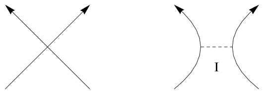
Figure 17: Smoothing according to a complex orientation

Proposition 3.7 (cf. [15, 11]).

Let $C_{1}$, $\ldots$, $C_{n}$ be nonsingular curves of degrees $d_{1}$, $\ldots$, $d_{n}$ in $\mathbb{RP}^{2}$ such that no three of them pass through the same point, and $C_{i}$ intersects transversally $C_{j}$ in $d_{i}d_{j}$ points for any $1\leq i<j\leq n$. Let ${\widetilde{C}}$ be a curve obtained by a small perturbation of the union $C_{1}\cup\ldots\cup C_{n}$ in such a way that all the imaginary intersection points of the curves $C_{1}$, $\ldots$, $C_{n}$ are kept, and all the real intersection points of these curves are smoothed. Assume that ${\widetilde{C}}$ is irreducible. Then, ${\widetilde{C}}$ is of type I if and only if all the curves $C_{1}$, $\ldots$, $C_{n}$ are of type I and there exists an orientation of ${\mathbb{R}}{\widetilde{C}}$ which agrees with some complex orientations of ${\mathbb{R}}C_{1}$, $\ldots$, ${\mathbb{R}}C_{n}$ (it means that the deformation turning $C_{1}\cup\ldots\cup C_{n}$ into ${\widetilde{C}}$ brings the chosen complex orientations of $C_{i}$ to the orientations of the corresponding pieces of ${\mathbb{R}}{\widetilde{C}}$ induced by a single orientation of the whole ${\mathbb{R}}{\widetilde{C}}$). In such case this orientation of ${\mathbb{R}}{\widetilde{C}}$ is one of the complex orientations of ${\widetilde{C}}$.

3.3 Rigid isotopies of nonsingular curves of degree $5$

Any curve of degree $5$ in $\mathbb{RP}^{2}$ is defined by a homogeneous real polynomial in three variables of degree $5$. The multiplication of this polynomial by a non-zero real constant gives rise to a polynomial defining the same curve. Thus, the space ${\mathbb{R}}{\mathcal{C}}_{5}$ of all curves of degree $5$ in $\mathbb{RP}^{2}$ can be identified with the real projective space of dimension $20$. The discriminant $\Delta\subset{\mathbb{R}}{\mathcal{C}}_{5}$ is formed by the points of ${\mathbb{R}}{\mathcal{C}}_{5}$ which correspond to singular curves. Two nonsingular curves of degree $5$ in $\mathbb{RP}^{2}$ are rigidly isotopic if the corresponding points belong to the same connected component of ${\mathbb{R}}{\mathcal{C}}_{5}\setminus\Delta$. It turns out that the rigid isotopy type of a nonsingular curve $C$ of degree $5$ in $\mathbb{RP}^{2}$ is determined by the topological arrangement of components of ${\mathbb{R}}C$ and the type (I or II) of $C$.

Theorem 3.8 (Kharlamov, see [10]).

There are nine rigid isotopy types of nonsingular curves of degree $5$ in $\mathbb{RP}^{2}$: $<J\sqcup 6>_{I}$, $<J\sqcup 5>_{II}$, $<J\sqcup 4>_{I}$, $<J\sqcup 4>_{II}$, $<J\sqcup 3>_{II}$, $<J\sqcup 2>_{II}$, $<J\sqcup 1>_{II}$, $<J>_{II}$, and $<J\sqcup 1<1>>_{I}$, where the subscript I or II indicates the type of curves.

We will need a more detailed information concerning the position of ovals of nonsingular curves of degree $5$ and type I. Let $C$ be a nonsingular curve of degree $5$ in $\mathbb{RP}^{2}$. Let $x_{1}$ and $x_{2}$ be two distinct points in $\mathbb{RP}^{2}\setminus J$, where $J$ is the pseudoline of ${\mathbb{R}}C$. The line passing through $x_{1}$ and $x_{2}$ intersects $J$ in odd number of points (if the line is not transversal to $J$, we count intersection points with multiplicities). Thus, exactly one of the two segments with endpoints $x_{1}$ and $x_{2}$ intersects $J$ in even number of points; we denote this segment by $[x_{1},x_{2}]_{C}$. A subset $S\subset(\mathbb{RP}^{2}\setminus J)$ is convex with respect to $C$ (or just convex if $C$ is understood), if for any two distinct points $x_{1}$ and $x_{2}$ belonging to $S$ the segment $[x_{1},x_{2}]_{C}$ is contained in $S$. If a subset $S^{\prime}\subset(\mathbb{RP}^{2}\setminus J)$ is contained in a convex subset of $\mathbb{RP}^{2}\setminus J$, then we can consider the convex hull of $S^{\prime}$, that is, the smallest convex set containing $S^{\prime}$.

Proposition 3.9.

Let $C$ be a nonsingular curve of degree $5$ in $\mathbb{RP}^{2}$ such that ${\mathbb{R}}C$ has at least three ovals. Let $x_{1}$, $x_{2}$, and $x_{3}$ be points in the interiors of three distinct ovals of ${\mathbb{R}}C$. Then, the union of the segments $[x_{1},x_{2}]_{C}$, $[x_{1},x_{3}]_{C}$, and $[x_{2},x_{3}]_{C}$ bounds a disc in $\mathbb{RP}^{2}\setminus J$. This disc is the convex hull of $x_{1}$, $x_{2}$, and $x_{3}$.

Proof.

The line passing through $x_{i}$ and $x_{j}$ (where $1\leq i<j\leq 3$) intersects ${\mathbb{R}}C$ transversally in $5$ points: two points of the oval whose interior contains $x_{i}$, two points of the oval whose interior contains $x_{j}$, and one point of $J$. Thus, the segment $[x_{i},x_{j}]_{C}$ does not intersect $J$. Since the union of our three segments does not intersect $J$, this union bounds a disc in $\mathbb{RP}^{2}\setminus J$. This disc coincides with one of the four triangles defined by the straight lines passing through $x_{1}$ and $x_{2}$, $x_{1}$ and $x_{3}$, $x_{2}$ and $x_{3}$. Clearly, it is convex and is contained in any convex set containing $x_{1}$, $x_{2}$, and $x_{3}$. ∎

The disc of Proposition 3.9 is called the triangle with vertices $x_{1}$, $x_{2}$, and $x_{3}$. Let $O_{1}$, $\ldots$, $O_{n}$, $n\geq 3$, be a collection of ovals of a nonsingular curve $C$ of degree $5$ in $\mathbb{RP}^{2}$, and let $x_{1}$, $\ldots$, $x_{n}$ be points in the interior of $O_{1}$, $\ldots$, $O_{n}$, respectively. We say that the ovals $O_{1}$, $\ldots$, $O_{n}$ are in convex position if for any choice of indices $1\leq i<j<k\leq n$, the triangle with vertices $x_{i}$, $x_{j}$, and $x_{k}$ does not contain in its interior any point $x_{1}$, $\ldots$, $x_{n}$. (Bézout theorem implies that the notion of convex position depends only on ovals $O_{1}$, $\ldots$, $O_{n}$ and not on the choice of points $x_{1}$, $\ldots$, $x_{n}$ inside these ovals.)

Proposition 3.10.

Let $C$ be a nonsingular curve of degree $5$ in $\mathbb{RP}^{2}$ such that ${\mathbb{R}}C$ has exactly four ovals. Then, these ovals are in convex position if and only if $C$ is of type II.

Proof.

The convexity of the position of four ovals of $C$ is invariant under rigid isotopies by Bézout theorem. Thus, Theorem 3.8 implies that, to prove the statement of the proposition, it is enough to construct

• a nonsingular curve $C_{1}$ of degree $5$ and type I in $\mathbb{RP}^{2}$ such that ${\mathbb{R}}C_{1}$ has exactly four ovals and these ovals are not in convex position, and

• a nonsingular curve $C_{2}$ of degree $5$ and type II in $\mathbb{RP}^{2}$ such that ${\mathbb{R}}C_{2}$ has exactly four ovals and these ovals are in convex position.

A construction of such curves is presented on Figure 18. The fact that the first curve is of type I and the second curve is of type II follows from Proposition 3.7. ∎

Figure 18: The construction of type I and II curves with 4 ovals from two ellipses and a line

Proposition 3.11.

Let $C$ be a nonsingular curve of degree $5$ in $\mathbb{RP}^{2}$ such that ${\mathbb{R}}C$ has at least five ovals. Then, the ovals of $C$ are in convex position.

Proof.

Let $x_{1}$, $\ldots$, $x_{5}$ be points in the interiors of five distinct ovals of ${\mathbb{R}}C$. There exists a unique conic $A$ which passes through the five points $x_{1}$, $\ldots$, $x_{5}$. Bézout theorem implies that this conic does not intersect $J$. The real part of $A$ is an oval, and the disc bounded by it is convex with respect to $C$. Thus, this disc contains the triangle with vertices $x_{i}$, $x_{j}$, and $x_{k}$ for any $1\leq i<j<k\leq 5$. In particular, the conic $A$ does not have points inside the triangle. ∎

Let $C$ be a nonsingular $M$-curve of degree $5$ in $\mathbb{RP}^{2}$, and let $O_{1}$, $\ldots$, $O_{6}$ be the ovals of ${\mathbb{R}}C$. Pick a point $x_{i}$ inside each oval $O_{i}$, $i=1$, $\ldots$, $6$. Points $x_{i}$ and $x_{j}$ are neighbors viewed from $x_{k}$ (where $O_{i}$ and $O_{j}$ are two distinct ovals of ${\mathbb{R}}C$, and $O_{k}$ is another oval of ${\mathbb{R}}C$) if

• one of the segments of the line pencil ${\cal L}^{k}_{i,j}$ connecting the lines $x_{k}x_{i}$ and $x_{k}x_{j}$ does not contain any line which intersects an oval different from $O_{i}$, $O_{j}$, $O_{k}$; denote this segment by ${\cal S}^{k}_{i,j}$;

• there is a path $\sigma^{k}_{i,j}\subset\mathbb{RP}^{2}$ connecting $x_{i}$ and $x_{j}$ such that any point of intersection of $\sigma^{k}_{i,j}$ with ${\mathbb{R}}C$ belongs either to $O_{i}$ or to $O_{j}$, each line of ${\cal S}^{k}_{i,j}$ intersects $\sigma^{k}_{i,j}$ in one point, and each line of ${\cal L}^{k}_{i,j}\setminus{\cal S}^{k}_{i,j}$ does not intersect $\sigma^{k}_{i,j}$.

Bézout theorem implies that, if $x_{i}$ and $x_{j}$ are neighbors viewed from $x_{k}$, then for any choice of points $x^{\prime}_{i}$, $x^{\prime}_{j}$, and $x^{\prime}_{k}$ inside the ovals $O_{i}$, $O_{j}$, and $O_{k}$, respectively, the points $x^{\prime}_{i}$ and $x^{\prime}_{j}$ are neighbors viewed from $x^{\prime}_{k}$. In this case, we say that the ovals $O_{i}$ and $O_{j}$ are neighbors viewed from $O_{k}$.

Lemma 3.12.

Let $C$ be a nonsingular $M$-curve of degree $5$ in $\mathbb{RP}^{2}$, and let $O_{1}$, $\ldots$, $O_{6}$ be the six ovals of ${\mathbb{R}}C$. Assume that $O_{i}$ and $O_{j}$ are neighbors viewed from $O_{k}$. Let $O_{n}$ and $O_{m}$ be two ovals different from $O_{i}$, $O_{j}$, and $O_{k}$. Then, the real part ${\mathbb{R}}A$ of the conic $A$ which passes through the points $x_{i}$, $x_{j}$, $x_{k}$, $x_{m}$, and $x_{n}$ contains an arc which have endpoints $x_{i}$, $x_{j}$ and does not contain any of the points $x_{k}$, $x_{m}$, $x_{n}$.

Proof.

The conic $A$ does not intersect $J$, and the points of ${\mathbb{R}}A$ are in a natural bijection with the lines of the pencil ${\cal L}^{k}$ centered at $x_{k}$. Thus, ${\mathbb{R}}A$ contains an arc $a$ with endpoints $x_{i}$, $x_{j}$ and such that $a$ does not contain any of the points $x_{m}$, $x_{n}$. Assume that $a$ contains the point $x_{k}$, and denote by $c_{i,j}$ the chord connecting $x_{i}$ and $x_{j}$ in the interior of ${\mathbb{R}}A$. There exists a path $\sigma^{k}_{i,j}\subset\mathbb{RP}^{2}$ connecting $x_{i}$ and $x_{j}$ and certifying that $O_{i}$ and $O_{j}$ are neighbors viewed from $O_{k}$. The union of $\sigma$ and $c_{i,j}$ is a cycle that intersects once each line of ${\cal L}^{k}$. Thus, this cycle is not homologous to $0\in H_{1}(\mathbb{RP}^{2};{\mathbb{Z}})$. Hence, the cycle constructed intersects $J$, which gives a contradiction. ∎

A reversible linear order (respectively, reversible cyclic order) on some collection of ovals is a pair of opposite linear (respectively, cyclic) orders on this collection.

Proposition 3.13.

Let $C$ be a nonsingular $M$-curve of degree $5$ in $\mathbb{RP}^{2}$, and let $O_{1}$, $\ldots$, $O_{6}$ be the six ovals of ${\mathbb{R}}C$.

1. For any oval $O_{k}$ of ${\mathbb{R}}C$, there exists a reversible linear order on the other five ovals of ${\mathbb{R}}C$ such that two ovals neighboring with respect to this reversible linear order are necessarily neighbors viewed from $O_{k}$.

2. If $O_{i}$ and $O_{j}$ are neighbors viewed from $O_{k}$, then $O_{i}$ and $O_{j}$ are neighbors viewed from any oval $O_{m}$ such that $m$ is different from $i$ and $j$.

3. If $O_{i}$ and $O_{j}$ are neighbors viewed from $O_{k}$, then one of the ovals $O_{i}$ and $O_{j}$ is positive, and the other one is negative.

Proof.

Pick a point $x_{i}$ inside each oval $O_{i}$, $i=1$, $\ldots$, $6$. The pseudoline $J$ of ${\mathbb{R}}C$ intersect each of the lines $x_{k}x_{i}$, $i=1$, $\ldots$, $6$, $i\neq k$, at exactly one point; denote this point by $y^{k}_{i}$. To prove the statement (a), notice that the line pencil ${\cal L}^{k}$ centered at $x_{k}$ provides a reversible cyclic order on the five ovals different from $O_{k}$. This pencil is formed by $5$ segments (with pairwise non-intersecting interiors), indexed by pairs of ovals $(O_{i},O_{j})$ which are neighbors with respect to this order; the segment $S^{k}_{i,j}$ indexed by $(O_{i},O_{j})$ connects the lines $x_{k}x_{i}$ and $x_{k}x_{i}$. For such a segment $S^{k}_{i,j}$, the ovals $O_{i}$ and $O_{j}$ are neighbors viewed from $O_{k}$ if and only if the orientations of the lines $x_{k}x_{i}$ and $x_{k}x_{j}$ provided by the triples of points $(x_{k},x_{i},y^{k}_{i})$ and $(x_{k},x_{j},y^{k}_{j})$, respectively, turn one to the one another through the segment $S^{k}_{i,j}$. Our purpose is to prove that, among the five segments $S^{k}_{i,j}$, there exists exactly one segment such that the corresponding ovals are not neighbors viewed from $O_{k}$. First, assume that there are two such segments $S^{k}_{i,j}$ and $S^{k}_{i^{\prime},j^{\prime}}$. Denote by $A$ the conic which passes through $x_{k}$, $x_{i}$, $x_{j}$, $x_{i^{\prime}}$, $x_{j^{\prime}}$ (in the case where the indices $i$, $j$, $i^{\prime}$, $j^{\prime}$ are not pairwise distinct, we choose an oval $O_{m}$ different from $O_{i}$, $O_{j}$, $O_{i^{\prime}}$, $O_{j^{\prime}}$, and suppose that $A$ passes through $x_{m}$). The five marked points divide the real part ${\mathbb{R}}A$ of $A$ into five arcs. Either $x_{i}$, $x_{j}$ or $x_{i^{\prime}}$, $x_{j^{\prime}}$ are endpoints of such an arc which contradicts the fact that $O_{i}$ and $O_{j}$, as well as $O_{i^{\prime}}$ and $O_{j^{\prime}}$, are not neighbors viewed from $O_{k}$. Furthermore, if any pair of ovals which are neighbors with respect to the reversible cyclic order provided by ${\cal L}^{k}$ are neighbors viewed from $O_{k}$, then we get five paths whose union is a cycle $c$ intersecting once each line of ${\cal L}^{k}$; the cycle $c$ is not homologous to $0\in H_{1}(\mathbb{RP}^{2};{\mathbb{Z}})$, thus $c$ intersects $J$.

To prove the statement (b), consider the segment $S$ of the line pencil connecting the lines $x_{m}x_{i}$ and $x_{m}x_{j}$ such that no line of $S$ intersects $O_{k}$, and assume that some line of $S$ intersects an oval $O_{n}$, where $n$ is different from $i$, $j$, $k$, and $m$. Trace a conic $B$ through the points $x_{i}$, $x_{j}$, $x_{k}$, $x_{m}$, and $x_{n}$. Since $O_{i}$ and $O_{j}$ are neighbors viewed from $O_{k}$, the real part ${\mathbb{R}}B$ of $B$ contains an arc $a$ such that its endpoints are $x_{i}$, $x_{j}$, and the interior of $a$ does not contain any of the points $x_{m}$, $x_{n}$, $x_{k}$ (see Lemma 3.12), which gives a contradiction.

To prove the statement (c), consider the segment ${\cal S}^{k}_{i,j}$ of the line pencil ${\cal L}^{k}_{i,j}$ connecting the lines $x_{k}x_{i}$ and $x_{k}x_{j}$ such that any line of ${\cal S}^{k}_{i,j}$ does not intersect any oval different from $O_{i}$, $O_{j}$, $O_{k}$. Orient all the real parts of the lines of the segment in such a way that the orientations turn to one another under the isotopy given by these real parts, and choose a complex orientation of ${\mathbb{R}}C$. Let $\widetilde{\cal S}^{k}_{i,j}$ be a subsegment of ${\cal S}^{k}_{i,j}$ such that the endpoints of $\widetilde{\cal S}^{k}_{i,j}$ correspond to lines tangent, respectively, to $O_{i}$ and $O_{j}$, and the interior points of $\widetilde{\cal S}^{k}_{i,j}$ correspond to lines which do not intersect any oval except $O_{k}$. The points $\widetilde{\cal S}^{k}_{i,j}$ which correspond to lines tangent to ${\mathbb{R}}C$ divide $\widetilde{\cal S}^{k}_{i,j}$ into segments $S_{1}$, $\ldots$, $S_{r}$ (each of these lines is tangent to ${\mathbb{R}}C$ at exactly one point). The endpoints of each of the segments $S_{1}$, $\ldots$, $S_{r}$ correspond to two tangency points $p$, $q$ of ${\mathbb{R}}C$ with lines of $\widetilde{\cal S}^{k}_{i,j}$; these two points are either both positive or both negative. Indeed, if the interior points of a segment $S_{t}$ under consideration correspond to lines intersecting ${\mathbb{R}}C$ at $3$ points, then the statement follows from Theorem 3.4. Assume that the interior points of a segment $S_{t}$ under consideration correspond to lines intersecting ${\mathbb{R}}C$ at $5$ points. Then, for each line corresponding to an interior point of $S_{t}$, either $3$ intersection points with ${\mathbb{R}}C$ belong to $J$ and the other two intersection points belong to $O_{k}$, or one intersection point belongs to $J$ and the other four intersection points belong to $O_{k}$. In the first case, Bézout theorem implies that $p$ and $q$ are connected by an arc $\alpha$ of $J$ such that $\alpha$ has exactly one common point with any line of $\widetilde{\cal S}^{k}_{i,j}$; furthermore, $p$ and $q$ are either both positive or both negative. In the second case, since $x_{k}$ is inside of $O_{k}$, the points $p$ and $q$ are connected by an arc $\beta$ of $O_{k}$ such that $\beta$ has exactly one common point with any line of $\widetilde{\cal S}^{k}_{i,j}$; furthermore, $p$ and $q$ are either both positive or both negative. ∎

Corollary 3.14.

Let $C$ be a nonsingular $M$-curve of degree $5$ in $\mathbb{RP}^{2}$. Then, there exists a reversible cyclic order of the six ovals of ${\mathbb{R}}C$ such that any two ovals which are neighbors with respect to this order are neighbors viewed from any other oval of ${\mathbb{R}}C$. This reversible cyclic order is invariant up to rigid isotopy of the curve; positive and negative ovals alternate with respect to this order. ∎

Remark 3.15.

Corollary 3.14 can as well be deduced from the rigid isotopy classification of nonsingular curves of degree $5$ in $\mathbb{RP}^{2}$ (Theorem 3.8), the fact that the existence of a reversible cyclic order required in the corollary is invariant under rigid isotopies, and a particular construction of a maximal curve of degree $5$ in $\mathbb{RP}^{2}$, for example, a small perturbation of three lines and an ellipse shown on Figure 19.

Figure 19: The construction of a $M$-curve from three lines and an ellipse

4 Tropical constructions

This section is devoted to the combinatorial patchworking and its tropical interpretation. The patchworking technique was invented by O. Viro at the end of the 1970’s. This technique provides a powerful tool to construct real plane algebraic curves (and, more generally, real algebraic hypersurfaces in toric varieties). We discuss here only certain particular cases of the general patchworking theorem.

4.1 Nodal tropical curves

We give here the definitions required for the combinatorial patchworking construction presented below. An introduction to tropical geometry and a detailed information on tropical curves can be found, for example, in [2]. A tropical curve in ${\mathbb{R}}^{2}$ is a finite weighted rectilinear graph $\Gamma$ in ${\mathbb{R}}^{2}$ (some of the edges of $\Gamma$ are not bounded) such that

• each edge $e$ of $\Gamma$ has a rational slope and prescribed a positive integer weight $w(e)$,

• at each vertex $v$ of $\Gamma$ the following balancing condition is satisfied:

  $$\sum_{e\supset v}w(e)u_{v}(e)=0,$$ (5)

  where the sum is taken over all edges $e$ adjacent to $v$, the vector $u_{v}(e)$ is the primitive integer vector (i.e., vector with integer relatively prime coordinates) in the direction of $e$ and pointing outward of $v$.

Consider the collection $\mathcal{C}$ of integer vectors $w(e)u_{v}(e)$ where $e$ runs over all non-bounded edges of $\Gamma$ and $v$ is the vertex adjacent to $e$. By (5) the sum of all vectors in the collection is zero. Thus, there exists a convex polygon $\Delta$ with integer vertices in ${\mathbb{R}}^{2}$ dual to this collection. This means that each vector $w(e)u_{v}(e)\in{\mathcal{C}}$ is an outward normal to a side $E\subset\Delta$ and

$$\#(E\cap{\mathbb{Z}}^{2})-1=\sum w(e),$$

where the sum is taken over all $w(e)u_{v}(e)\in{\mathcal{C}}$ that are outward normal vectors to $E$. The polygon $\Delta$ is called Newton polygon of $\Gamma$. It is defined up to translation. The quantity $\#(E\cap{\mathbb{Z}}^{2})-1$ is called the integer length of the interval $E$ (recall that the endpoints of $E$ are from ${\mathbb{Z}}^{2}$).

If $\Delta$ can be chosen to coincide with the triangle with vertices $(0,0)$, $(d,0)$, $(0,d)$ for some positive integer $d$, then we say that $\Gamma$ is projective of degree $d$. The latter means that each vector $u_{v}(e)$, where $e$ is a non-bounded edge of $\Gamma$, is either $(-1,0)$, or $(0,-1)$, or $(1,1)$, and the number of such vectors (counted with weights $w(e)$) in each direction is equal to $d$.

A tropical curve $\Gamma$ in ${\mathbb{R}}^{2}$ is said to be irreducible, if it cannot be presented as a union of two tropical curves different from $\Gamma$.

The space ${\mathcal{T}}(\Delta)$ of tropical curves with a given Newton polygon $\Delta\subset{\mathbb{R}}^{2}$ is equipped with a natural topology induced by the Hausdorff distance

$$d(\Gamma_{1},\Gamma_{2})=\max\{\sup_{p\in\Gamma_{1}}\inf_{q\in\Gamma_{2}}\text{\rm dist}(p,q),\ \sup_{q\in\Gamma_{2}}\inf_{p\in\Gamma_{1}}\text{\rm dist(p, q)}\},$$

where $\text{\rm dist}(p,q)$ is the Euclidean distance between points $p$ and $q$. The condition that $\Gamma_{1}$ and $\Gamma_{2}$ have the same Newton polygon ensures finiteness of this distance.

A tropical curve $\Gamma$ in ${\mathbb{R}}^{2}$ is said to be nonsingular if

• each edge of $\Gamma$ is of weight $1$,

• each vertex $v$ of $\Gamma$ is $3$-valent and the primitive integer vectors in the directions of three edges adjacent to $v$ generate (over ${\mathbb{Z}}$) the lattice ${\mathbb{Z}}^{2}\subset{\mathbb{R}}^{2}$ of vectors with integer coordinates.

A tropical curve $\Gamma$ in ${\mathbb{R}}^{2}$ is said to be nodal (or simple, cf. [13]) if

• each vertex of $\Gamma$ is either $3$-valent or $4$-valent,

• for each $4$-valent vertex of $\Gamma$, the union of four edges adjacent to this vertex is contained in a union of two straight lines.

For our constructions, we use some particular degenerations of nonsingular tropical curves to nodal ones. These degenerations contract certain edges of nonsingular tropical curves in ${\mathbb{R}}^{2}$, as well as some ”triangles”. A triangle in a nonsingular tropical curve $\Gamma$ in ${\mathbb{R}}^{2}$ is a collection of three edges of $\Gamma$ which form a cycle such that no vertex of $\Gamma$ is inside this cycle.

Let $\Delta\subset{\mathbb{R}}^{2}$ be a convex polygon with integer vertices, and let $\gamma:\to{\mathcal{T}}(\Delta)$ be a path such that

• $\gamma(t)$ is a nonsingular tropical curve for any $t\in(0,1]$;

• $\gamma(0)$ is a nodal tropical curve;

• the underlying graph of the tropical curve $\gamma(0)$ can be obtained from the underlying graph of $\gamma(t)$ for any $t\in(0,1]$ by contraction of a collection ${\mathcal{C}}_{\text{\rm edges}}$ of pairwise disjoint edges (i.e., no two edges of ${\mathcal{C}}_{\text{\rm edges}}$ have common endpoint) and a collection ${\mathcal{C}}_{\text{\rm triangles}}$ of pairwise disjoint triangles (i.e., no two edges of different contracted triangles have common endpoint); furthermore, no edge of ${\mathcal{C}}_{\text{\rm edges}}$ has common endpoint with any edge of the contracted triangles.

In this case, we say that the nodal tropical curve $\gamma(0)$ is an immediate degeneration of $\gamma(1)$ (and $\gamma(1)$ is an immediate perturbation of $\gamma(0)$).

4.2 Combinatorial patchworking of real nodal curves

Let $\Gamma$ be a nonsingular tropical curve in ${\mathbb{R}}^{2}$. A real structure on $\Gamma$ is given by a collection $T$ of bounded edges of $\Gamma$ which satisfy the following condition:

• for any cycle of $\Gamma$, denote by $e_{1}$, $\ldots$, $e_{\ell}$ the edges of the cycle that belong to $T$; then, one has

  $$\sum_{i=1}^{\ell}u_{i}=0\quad\text{mod }2,$$ (6)

  where $u_{1},\ldots,u_{\ell}$ are primitive integer vectors in the directions of $e_{1}$, $\ldots$, $e_{\ell}$, respectively.

Such a collection $T$ is called twist-admissible, and the edges of $T$ are called twisted.

To each nonsingular tropical curve $\Gamma$ in ${\mathbb{R}}^{2}$ and each twist-admissible collection $T$ of edges of $\Gamma$ we associate a smooth curve $C(\Gamma,T)\subset({\mathbb{R}}^{\times})^{2}$ using the following procedure.

• At each vertex of $\Gamma$, we draw three arcs as depicted in Figure 20.

  Figure 20: Three arcs at a vertex

• For each bounded edge $e$ of $\Gamma$ we join the two corresponding arcs of one endpoint of $e$ to the two corresponding arcs of the other endpoint of $e$ in the following way: if $e\notin T$, then join these arcs as depicted in Figure 21; if $e\in T$, then join these arcs as depicted in Figure 22. Denote by ${\widetilde{C}}(\Gamma,T)$ the curve obtained.

  Figure 21: Arcs for an edge which does not belong to $T$

  Figure 22: Arcs for an edge which belongs to $T$

• Choose arbitrarily a branch of ${\widetilde{C}}(\Gamma,T)$ and a pair of signs (each sign being $+$ or $-$) for this branch.

• Associate pairs of signs to all branches of ${\widetilde{C}}(\Gamma,T)$: for each edge $e$ with primitive integer direction $(u_{1},u_{2})$, the pairs of signs of the two branches of ${\widetilde{C}}(\Gamma,T)$ corresponding to $e$ differ by the factor $((-1)^{u_{1}},(-1)^{u_{2}})$. The compatibility condition (6) ensures that the rule is consistent.

• Map each branch of ${\widetilde{C}}(\Gamma,T)$ to $({\mathbb{R}}^{\times})^{2}$ by $(x,y)\mapsto(\epsilon_{1}e^{x},\epsilon_{2}e^{y})$, where $(\epsilon_{1},\epsilon_{2})$ is the pair of signs associated to the branch. Denote by $C(\Gamma,T)$ the union of the images of all branches of ${\widetilde{C}}(\Gamma,T)$.

The isotopy type of the curve $C(\Gamma,T)\subset({\mathbb{R}}^{\times})^{2}$ is determined by $\Gamma$ and $T$ up to axial symmetries.

If $\Gamma$ has $\Delta$ as Newton polygon, denote by ${\overline{C}}(\Gamma,T)$ the closure of $C(\Gamma,T)\subset({\mathbb{R}}^{\times})^{2}\subset{\mathbb{R}}Tor(\Delta)$ in the real part ${\mathbb{R}}Tor(\Delta)$ of the toric surface $Tor(\Delta)$ associated with $\Delta$. In particular, if $\Gamma$ is of projective degree $d$, then ${\overline{C}}(\Gamma,T)\subset\mathbb{RP}^{2}$.

An algebraic curve $A$ in $({\mathbb{R}}^{\times})^{2}$ is a real Laurent polynomial in two variables well-defined up to multiplication by a monomial. Such a polynomial has a zero locus in ${\mathbb{R}}A\subset({\mathbb{R}}^{\times})^{2}$. The Newton polygon $\Delta$ of the polynomial is also called the Newton polygon of $A$. Denote with ${\mathbb{R}}\bar{A}$ the closure of ${\mathbb{R}}A$ in $Tor(\Delta)$.

The combinatorial patchworking (a particular case of the Viro patchworking theorem [22]) can be reformulated in terms of twist-admissible collections as follows.

Theorem 4.1 (cf. [22]).

Let $\Gamma$ be a nonsingular tropical curve in ${\mathbb{R}}^{2}$, and let $\Delta$ be a Newton polygon of $\Gamma$. Then, for any twist-admissible collection $T$ of $\Gamma$, there exists a nonsingular real algebraic curve $A$ in $({\mathbb{R}}^{\times})^{2}$ of Newton polygon $\Delta$ such that the pairs $(({\mathbb{R}}^{\times})^{2},{\mathbb{R}}A)$ and $(({\mathbb{R}}^{\times})^{2},C(\Gamma,T))$ are homeomorphic. Furthermore, the pairs $({\mathbb{R}}Tor(\Delta),{\mathbb{R}}\bar{A})$ and $({\mathbb{R}}Tor(\Delta),{\overline{C}}(\Gamma,T))$ are also homeomorphic.

E.g. if $\Gamma$ is projective degree $d$, then there exists a nonsingular curve ${\mathbb{R}}{\overline{A}}$ of degree $d$ in $\mathbb{RP}^{2}$ such that the topological pairs $(\mathbb{RP}^{2},{\mathbb{R}}{\overline{A}})$ and $(\mathbb{RP}^{2},{\overline{C}}(\Gamma,T))$ are homeomorphic. A reformulation similar to Theorem 4.1 was used by B. Haas in [6] for characterization of M-curves obtained by combinatorial patchworking.

Notice that the empty collection of edges is always twist-admissible. The resulting nonsingular real algebraic curves are called simple Harnack curves. They were introduced in [12].

Let $\Gamma$ be a nonsingular tropical curve in ${\mathbb{R}}^{2}$, and let $\Gamma^{\prime}$ be an immediate degeneration of $\Gamma$ which is a nodal tropical curve. Then, the underlying graph of $\Gamma^{\prime}$ is obtained from the underlying graph of $\Gamma$ by contracting a collection ${\mathcal{C}}_{\text{\rm edges}}=\{e_{1},\ldots,e_{r}\}$ of pairwise-disjoint edges as well as a collection ${\mathcal{C}}_{\text{\rm triangles}}=\{tr_{1},\ldots,tr_{s}\}$ of triangles. Suppose that $\Gamma$ is enhanced with such a real structure that all $e_{j}$, $j=1,\dots,r$, are twisted while all the triangles $tr_{j}$, $j=1,\dots,s$, are composed of non-twisted edges. For each $i=1$, $\ldots$, $r$, the curve $C(\Gamma,T)$ contains two arcs $a_{i}$ and $b_{i}$ which are associated with two endpoints of $e_{i}$ but correspond to edges different from $e_{i}$ (in Figure 22 such arcs are shown in red). The condition (6) implies that these two arcs are contained in the same quadrant of $({\mathbb{R}}^{\times})^{2}$. Furthermore, for each $j=1$, $\ldots$, $s$, the curve $C(\Gamma,T)$ contains an oval $o_{j}$ corresponding to the triangle $tr_{j}$. Denote by $C^{\prime}(\Gamma,T,{\mathcal{C}}_{\text{\rm edges}},{\mathcal{C}}_{\text{\rm triangles}})\subset({\mathbb{R}}^{\times})^{2}$ the subset obtained from the curve $C(\Gamma,T)$ by replacing each pair of arcs $a_{i}$, $b_{i}$ with a ”cross” as in Figure 23 and contracting each oval $o_{j}$ (where $j=1$, $\ldots$, $s$) to a point as in Figure 24. The isotopy type of $C^{\prime}(\Gamma,T,{\mathcal{C}}_{\text{\rm edges}},{\mathcal{C}}_{\text{\rm triangles}})\subset({\mathbb{R}}^{\times})^{2}$ is determined up to axial symmetries by the tropical curve $\Gamma$, the real structure $T$, and the collections ${\mathcal{C}}_{\text{\rm edges}}$ and ${\mathcal{C}}_{\text{\rm triangles}}$. Once again, if $\Gamma$ has $\Delta$ as Newton polygon, denote by ${\overline{C}}^{\prime}(\Gamma,T,{\mathcal{C}}_{\text{\rm edges}},{\mathcal{C}}_{\text{\rm triangles}})$ the closure of $C^{\prime}(\Gamma,T,{\mathcal{C}}_{\text{\rm edges}},{\mathcal{C}}_{\text{\rm triangles}})$ in ${\mathbb{R}}Tor(\Delta)$.

Figure 23: Replacing two arcs by a ”cross”

Figure 24: Contracting an oval

The following theorem is a corollary of the Viro patchworking theorem [22] for an appropriate $(r+s)$-dimensional family of curves. It also can be viewed as a special case of [17].

Theorem 4.2 (cf. [22]).

Let $\Gamma$ be a nonsingular tropical curve of Newton polygon $\Delta$ in ${\mathbb{R}}^{2}$, and let $\Gamma^{\prime}$ be a nodal tropical curve obtained as an immediate degeneration of $\Gamma$. Denote by ${\mathcal{C}}_{\text{\rm edges}}$ (respectively, ${\mathcal{C}}_{\text{\rm triangles}}$) the collection of edges (respectively, of triangles) of $\Gamma$ that are contracted in the degeneration of $\Gamma$ to $\Gamma^{\prime}$.

Then, for any twist-admissible collection $T$ of $\Gamma$ such that ${\mathcal{C}}_{\text{\rm edges}}\subset T$ and no edge of the triangles in ${\mathcal{C}}_{\text{\rm triangles}}$ is in $T$, there exists a nodal real algebraic curve ${\mathbb{R}}A\subset({\mathbb{R}}^{\times})^{2}$ with Newton polygon $\Delta$ and $r+s$ nodes such that the pairs $(({\mathbb{R}}^{\times})^{2},C^{\prime}(\Gamma,T,{\mathcal{C}}_{\text{\rm edges}},{\mathcal{C}}_{\text{\rm triangles}}))$ and $(({\mathbb{R}}^{\times})^{2},{\mathbb{R}}A)$ are homeomorphic. Furthermore, the pairs $({\mathbb{R}}Tor(\Delta),\overline{C}^{\prime}(\Gamma,T,{\mathcal{C}}_{\text{\rm edges}},{\mathcal{C}}_{\text{\rm triangles}}))$ and $({\mathbb{R}}Tor(\Delta),{\mathbb{R}}\bar{A})$ are also homeomorphic; if in addition $\Gamma$ is irreducible, then ${\overline{A}}$ can be chosen irreducible.

5 Restrictions

In this section, we start the proof of theorem 1.10. In fact, we obtain a more detailed classification of nodal rational curves of degree $5$ in $\mathbb{RP}^{2}$: we describe all possible complex schemes of these curves. The complex scheme of a nodal rational curve $C$ in $\mathbb{RP}^{2}$ is the topological type of the pair $(\mathbb{RP}^{2},{\mathbb{R}}C)$ equipped with one of two complex orientations of ${\mathbb{R}}C$. Recall that given a half of the normalization $\psi:\widehat{C}\to C$, we get a complex orientation for each elliptic node $p\in{\mathbb{R}}C$ that is the local orientation of $\mathbb{RP}^{2}$ at $p$ such that the intersection at $p$ of $\mathbb{RP}^{2}$ and the image under $\psi$ of the chosen half is positive.

5.1 Possible complex schemes of small perturbations

Let $C$ be a nodal rational curve of degree 5 in $\mathbb{RP}^{2}$, and let $C_{\circ}$ be a small perturbation of $C$ (see Brusotti’s theorem 3.5), such that all hyperbolic nodes are smoothed according to the complex orientations, each elliptic node is smoothed into an oval, and all complex conjugated nodes are kept. Since $C$ is of type I, the perturbation $C_{\circ}$ is also of type I (see Proposition 3.6). Furthermore, the complex orientations of ${\mathbb{R}}C_{\circ}$ are induced by the complex orientations of ${\mathbb{R}}C$. Denote by $l$ the number of connected components of ${\mathbb{R}}C_{\circ}$. Recall that $\sigma$ stands for the number of imaginary nodes of $C$ resulted as the intersection of the images of ${\widehat{C}}_{+}$ and ${\widehat{C}}_{-}$ under the normalization map $\psi:\widehat{C}\to C$, where ${\widehat{C}}_{\pm}$ are the two connected components of ${\mathbb{C}}\widehat{C}\setminus{\mathbb{R}}{\widehat{C}}$.

Proposition 5.1.

The complex scheme of $C_{\circ}$ is one of the seven schemes listed in the table 5.1. Moreover,

• if $l=7$, then $C_{\circ}$ is a nonsingular $M$-curve, and hence satisfies the convexity properties 3.11, 3.12, 3.13, 3.14,

• if $l=5,\sigma=0$, the single positive oval of ${\mathbb{R}}C_{\circ}$ is contained in the triangle formed by the three negative ovals (in particular, the four ovals are in non-convex position),

• if $l=5,\sigma=2$, then the four ovals of ${\mathbb{R}}C_{\circ}$ are in convex position.

$\sigma$	$l$	7	5	3	1
0

& 2 4 6

Table 8: Seven possible complex schemes of ${\mathbb{R}}C_{\circ}$

Proof.

The numbers $l,h,e,c,\sigma$ satisfy some straightforward relations. First, we have $h+e+c=6$, the total number of nodes of $C$. Second, from lemma 2.9 and the fact that each elliptic node gives rise to an oval of ${\mathbb{R}}C_{\circ}$ we can deduce that $l$ is odd and $1+e\leq l\leq 7-c$ (as $6-c$ is the number of real nodes of $C$). Moreover, we obviously have $0\leq\sigma\leq c$. These inequalities explain the upper-triangular shape of the table. Let us now smooth the complex conjugated nodes of $C_{\circ}$ in order to obtain a nonsingular curve $C^{\prime}$. Note that $C^{\prime}$ is of type I if and only if $\sigma=0$. Therefore, according to the rigid isotopy classification 3.8, the complex scheme of ${\mathbb{R}}C^{\prime}$, and hence also the complex scheme of ${\mathbb{R}}C_{\circ}$, is completely determined by $l$ and $\sigma$, namely $<J\sqcup 6>_{I}$, $<J\sqcup 4>_{I}$ or $<J\sqcup 1<1>>_{I}$ for $\sigma=0$ and $<J\sqcup 4>_{II}$, $<J\sqcup 2>_{II}$ or $<J>_{II}$ for $\sigma\neq 0$. As explained before, $C_{\circ}$ is of type I by Proposition 3.6 and therefore satisfies the complex orientation formula 3.3. Applied to our case, when $l$ and $\sigma$ are fixed, this formula in fact uniquely determines the complex orientations, as depicted in table 5.1. In particular, if $l=1$ the formula implies $\sigma=6$. Finally, the convexity statements follow from the corresponding statements for $C^{\prime}$ (using proposition 3.10). In the non-convex case, we also use Fiedler’s alternation rule 3.4. Consider a triangle spanned by three ovals and containing the fourth one. Applying 3.4 to a pencil of lines with base point in the fourth oval, for example, we see that the three outer ovals must have the same orientation. This finishes the proof. ∎

In what follows, we go through these seven cases and study which smoothing diagrams we can get for each complex scheme.

5.2 General restrictions on smoothing diagrams

Let $\Delta_{C}=(C_{\circ};\;\bigcup_{p}I_{p})$ be a smoothing diagram of real nodal rational curve $C$ of degree $5$ in $\mathbb{RP}^{2}$. As above, $C_{\circ}$ is a type I small perturbation of $C$ and $\bigcup_{p}I_{p}$ is a union of $h$ vanishing cycles. The following pieces of terminology will be useful.

Definition 5.2.

Let $\Delta=(L;I)$ be a smoothing diagram (cf. Definition 2.7). A connected component of $L$ which does not intersect any of the vanishing cycles in $I$ is called an isolated oval. Let $\Delta^{*}$ be the smoothing diagram obtained from $\Delta$ after removing all isolated ovals. We call $\Delta$ irreducible if $\Delta^{*}$ is the smoothing diagram of a single immersed circle (cf. Proposition 2.8).

The following proposition recollects straightforward properties of smoothing diagrams of real rational curves (cf. discussions in subsections 2.2 and 2.3).

Proposition 5.3.

The smoothing diagram $\Delta_{C}$ satisfies the following properties.

1. The underlying graph $\Gamma(\Delta_{c})$ has $e$ isolated vertices and one further connected component with $h+e+1-l=7-c-l$ cycles.

2. All vanishing cycles of $\Delta_{C}$ are coherent (cf. Definition 2.7). This means that a vanishing cycle $I_{p}$ connects either

   • the pseudoline and a negative oval,

   • or a positive and a negative oval, if they are unnested,

   • or a negative injective pair of ovals.

3. The smoothing diagram $\Delta_{C}$ is irreducible (cf. Definition 5.2).

4. The interior of any isolated oval is empty.

In addition to these purely topological properties, further general restrictions in the case of algebraic curves are provided, by the Bézout theorem. To formulate these restrictions, we introduce the concept of a quasiline. Let $\Delta=(C_{\circ};\;\bigcup_{p}I_{p})$ be a smoothing diagram, and let $L$ be a non-contractible smoothly embedded closed 1-submanifold of ${\mathbb{R}}{\mathbb{P}}^{2}$. We say that $L$ is a quasiline with respect to $\Delta$ if the following conditions hold:

• The intersection of $L$ and $C_{\circ}$ is transverse,

• for each (closed) interval $I_{p}$, we have either $|L\cap I_{p}|\leq 1$ or $L\cap I_{p}=I_{p}$, in the former case $L$ and $I_{p}$ intersect transversally, and $L$ is disjoint from the endpoints of $I_{p}$,

• let $r$ be the number of intervals $I_{p}$ with $L\cap I_{p}\neq\emptyset$, and let $s$ be the cardinality of the intersection $L\cap(C_{\circ}\setminus\bigcup_{p}I_{p})$; then

  $$L.\Delta:=2r+s\leq 5.$$ (7)

Lemma 5.4.

Let $\Delta_{C}=(C_{\circ};\;\bigcup_{p}I_{p})$ be a smoothing diagram of real nodal rational curve $C$ of degree $5$ in $\mathbb{RP}^{2}$. Then, for any two points $p_{1},p_{2}\in{\mathbb{R}}{\mathbb{P}}^{2}$, there exists a quasiline with respect to $\Delta_{C}$ passing through the points. If several pairs of points are given, all these quasilines can be chosen in such a way that any two of them intersect either in a single point transversally or along a single interval $I_{p}$.

Proof.

Let $C^{t},t\in[0,1]$ be family of curves such that $C^{0}=C$, $C^{1}=C_{\circ}$, and such that for $t>0$ this family forms an rigid isotopy. Let us fix small discs $D$ around the hyperbolic nodes of $C$. Then there exists $s\in(0,1]$ such that the intersection of any of the discs $D$ with ${\mathbb{R}}C^{t}$ for $t\in(0,s]$ consists of two embedded intervals. Let $I_{p}^{t}$ be a corresponding family of vanishing cycles connecting these intervals such that $I_{p}^{0}=\{p\}$ is a node of $C$. Then, for each $t\in(0,s]$, the tuple $({\mathbb{R}}C^{t};\bigcup_{p}I^{t}_{p})$ is equivalent to $\Delta_{C}$ up to isotopy. For each point $p_{i}$ appearing in the statement, we choose a path $p_{i}^{t}$ such ${\mathbb{R}}C^{t}\cup\bigcup_{p}I_{p}\cup p^{t}_{i}$ is isotopic to $\Delta_{C}\cup p_{i}$ for all $t\in(0,s]$. In particular, if $p_{i}\in I_{p}$, then $p_{i}^{0}$ coincides with the corresponding node $p$ of $C$. Let us now prove the existence of quasilines through $p_{1},p_{2}$. Start with the (honest) lines $L^{t}:=\overline{p_{1}^{t}p_{2}^{t}}$. By Bézout’s theorem, we have $|{\mathbb{R}}L^{0}\cap{\mathbb{R}}C|\leq 5$. We would like to show that $L^{t}.({\mathbb{R}}C^{t};\;\bigcup_{p}I_{p})\leq|{\mathbb{R}}L^{0}\cap{\mathbb{R}}C|$. As we consider small perturbations of $C$ and $L^{0}$, the statement is clear if $L^{0}$ does not contain any hyperbolic node of $C$. Hence, assume that $p\in L^{0}$ is a hyperbolic node of $C$, and let $D$ be the disc around $p$. Suppose first that $L_{0}$ intersects both branches of $C$ at $p$ transversally (so that the local intersection multiplicity is $m_{p}=2$). Depending on whether the two points which form the intersection of $L^{t}$ with the boundary $\partial D$ of $D$ are connected in $D\setminus C^{t}$ or not, we may replace the segment $L^{t}\cap D$ by a path which intersects $I_{p}$ in a single point or a path which contains $I_{p}$. In both cases, the local contribution to (7) is $2$, so we constructed a quasiline with the required properties. For $m_{p}>2$, note that any two points in $\partial D\setminus C_{t}$ can be joined via a path traversing or containing $I_{p}$ with local contribution to (7) less than $3$. Finally, the statement about several lines obviously follows from the fact that two (honest) lines intersect in a single point. Indeed, even if this intersection point is a node of $C$, the above procedure can be performed such that the two paths intersect either in a single point or in the interval $I_{p}$. ∎

Remark 5.5.

Similarly, we can show the following statement: Given an interval $I_{p}$, there exists

• a quasiline intersecting the interval $I_{p}$ transversally in a single interior point,

• a quasiline containing the interval.

This corresponds to choosing $L_{0}$ to be a line intersecting the corresponding node transversally and lying in the corresponding “quadrants of the node”. Clearly, we may assume that the pairwise intersections of such quasilines are also either single points or the interval $I_{p}$ itself.

5.3 $M$-curve case ($l=7$)

In the M-curve case $l=7$, we have $\sigma=c=0$, and all necessary further restrictions can be summarized in Proposition 5.6 below. Let $\Delta$ be the following diagram (in the sense of definition 2.7):

A subdiagram of $\Delta$ is a diagram obtained from $\Delta$ by removing some of the (dashed) intervals. A diagram $\Delta^{\prime}$ is called a tree (or arboreal cf. Definition 2.30) if the underlying graph $\Gamma(\Delta)$ is a (connected) tree plus possibly some isolated points.

Proposition 5.6.

If $l=7$ (i.e. if $C_{\circ}$ is a M-curve), then the smoothing diagram $\Delta_{C}$ is (up to isotopy) a subtree of $\Delta$. Moreover, table 3 lists all 32 possible choices of such subtrees.

Proof.

We will prove the following properties of $\Delta_{C}$ which, together with corollary 3.14, imply the statement.

1. $\Delta_{C}$ is a tree (in particular, it does not have double edges or loops).

2. Two ovals connected by a vanishing cycle must be neighbors in the sense of subsection 3.3.

3. An oval connected to the pseudoline of $C_{\circ}$ by a vanishing cycle must be negative.

4. Assume that there are three vanishing cycles attached to the pseudoline of $C_{\circ}$. Then when moving along $J$, the vanishing cycles lie on alternating sides.

Part (a) follows from Proposition 5.3 (a). For (b), let us consider two ovals $O_{1}$ and $O_{2}$ connected by a vanishing cycle. Let $O_{3}$ be an arbitrary third oval of $C_{\circ}$, and let $x_{1},x_{2},x_{3}$ be points in their respective interiors. We want to show that $x_{1}$ and $x_{2}$ are neighbors viewed from $x_{3}$ according to the definition on page 3.3. To do so, we define the path $\sigma_{1,2}^{3}$ to be the line segment $[x_{1},x_{2}]_{C_{\circ}}$ and we define ${\cal S}^{k}_{i,j}$ to be the segment of the pencil of lines through $x_{3}$ which intersect $[x_{1},x_{2}]_{C_{\circ}}$. With these choices, the second condition for being neighbors is obviously satisfied, and it remains to show that the lines in ${\cal S}^{k}_{i,j}$ do not intersect any other oval than $O_{1},O_{2},O_{3}$. For this we might have to replace $C_{\circ}$ by a deformation which is sufficiently close to $C$. More precisely, let $C^{t},t\in[0,1]$ be family of curves such that $C^{0}=C$, $C^{1}=C_{\circ}$, and such that for $t>0$ this family forms an rigid isotopy. We can proceed as above for each $t$, with the additional assumption that the chosen points $x^{t}_{1},x^{t}_{2}$ converge to the node $p$ when $t$ goes to $0$. We now want to show that the lines in the segment ${\cal S}^{k,t}_{i,j}$ do not intersect any other oval of $C^{t}$ for sufficiently small $t$. If this was not true, when $t$ goes to $0$ this would imply the existence of a line passing through $p$ and at least two other ovals/nodes of $C$, which contradicts the Bézout theorem. Part (c) immediately follows from Proposition 5.3 (b). For (d), let us choose a point in the interior of each positive oval of $C_{\circ}$, and consider the three straight lines passing each through two of the chosen points. These three lines divide $\mathbb{RP}^{2}$ in four regions. One of these regions is the convex triangle with vertices at the chosen points. Propositions 3.11 and 3.13 imply that each of the three other regions contains a negative oval of $C_{\circ}$. Furthermore, each of these three regions is cut by the pseudoline of $C_{\circ}$ into two sub-regions. We call such a sub-region triangular (respectively, quadrangular) if it is adjacent to two (respectively, three) straight lines passing through the chosen points. Proposition 3.13 implies that each negative oval of $C_{\circ}$ is contained in a quadrangular sub-region. As in the proof of part (b) the vanishing cycles must be disjoint from our three straight lines. Thus the three quadrangular sub-regions are adjacent to the pseudoline from alternating sides, which finishes the proof.

∎

5.4 The Hyperbolic Curve ($l=3,\sigma=0$)

Let us now consider smoothing diagrams which are based on a hyperbolic curve (i.e. $l=3,\sigma=0$). By Proposition 5.3 (b), such a smoothing diagrams has vanishing cycles of two types, connecting the pseudoline and the outer oval or connecting the nested ovals. For now, let us remove the latter ones and classify the remaining diagrams up to isotopy. For this it is useful to use the language of immersion graphs from Definition 2.19 (even though for visual convenience we stick to more intuitive smoothing diagrams in the pictures). In our situation (after removing the inner oval and adjacent vanishing cycles), we are left with immersion graphs $\Gamma$ on two vertices: the root vertex $w$ and a second vertex $v$. All edges are directed from $v$ to $w$. The number of edges is $1\leq t\leq 5$. The ribbon structure of $\Gamma$ gives us two cyclic orderings of the edges. Finally, the projective enhancement of $\Gamma$ (the crosses on the segments of $w$) can be encoded in a vector $T\in{\mathbb{Z}}_{2}^{t}$, which contains an entry $1$ for each crossed segment. This vector $T$ is well-defined up to cyclic reordering and if $|T|$ denotes the sum of the entries of $T$, we have

$$|T|\equiv 1\mod 2.$$ (8)

From the compatibility property of the two cyclic orderings in proposition 2.25 it follows that $\Gamma$ is in fact completely determined by $T$. Moreover, by proposition 2.27 the isotopy type of the reduced smoothing diagram is determined by $\Gamma$. Hence the list of possible reduced smoothing diagrams corresponds to the list of possible vectors $T$ and looks as follows.

Given such a reduced diagram, the outer oval is subdivided into $t$ segments. Again by proposition 2.25, the isotopy type of the full diagram is determined by the data to which segments the $h-t$ “inner” vanishing cycles are attached.

Many of the choices for attaching the vanishing cycles are prohibited by the irreducibility condition of Proposition 5.3 (c). The typical situation is depicted in the following picture.

It shows a component $K$ together with a sequence $p_{0},p_{1},\ldots,p_{n}=p_{0}$ of pairs of vanishing cycles $p_{i}=\{I_{i},I^{\prime}_{i}\}$ attached to it. Each pair $p_{i}$ connects $K$ to the same component $K_{i}$. Moreover, the vanishing cycles following $I^{\prime}_{i}$ with respect to the cyclic ordering on $K$ is $I_{i+1}$, and the vanishing cycles following $I_{i}$ with respect to the cyclic ordering on $K_{i}$ is $I^{\prime}_{i}$ (as indicated by the bold segments here). Such a diagram violates Proposition 5.3 (c), as the bold segments together with the vanishing cycles form an embedded circle which does not cover the whole curve. We refer to this situation by $(Red)$. Note that $K$ can be any component of $C_{\circ}$, even though we depicted it as an oval in the picture.

We now list all diagrams which satisfy to the properties listed in Proposition 5.3 (in particular, to the $(Red)$-rule). As explained above, given a reduced diagram from the above the list, we need to specify to which segments the “inner” vanishing cycles are attached. Of course, it suffices to consider these choices up to symmetries of the reduced diagram. For example, for $T=(0,0,1)$, the two “lower” segments of the outer oval are symmetric. Note that by Proposition 5.3 (d) we have $e=0,1$ (only the inner oval can correspond to an elliptic node). Let us start with $e=0$.

We start with the case $e=0$ and go through all possible choices for $T$. For $T=(1)$, there is only one segment to choose, so we get the following three types.

&

For $T=(0,1)$, there are two segments to choose from. Note that assigning an even number of vanishing cycles to each of the segments is forbidden $(Red)$. All other options are depicted below.

&

For $T=(0,0,1)$, we get three segments, two of which are symmetric. All choices satisfy to Proposition 5.3, except for attaching one vanishing cycle to each segment (such a smoothing diagram violates the irreducibility condition (c)).

& $c=2$

For $T=(1,1,1)$, all three segments are symmetric. Note also that in this case, the reduced diagram itself is not irreducible in the sense of Proposition 5.3 (c), but consists of three components containing one of the segments each. In particular, the completed diagram can satisfy to the condition (c) only if the additional vanishing cycles are attached to all the three segments. Hence, the only possible type is as follows:

From now on we assume that $t\geq 4$ (hence $c=0$). For $T=(0,0,0,1)$, we get a $(Red)$-situation whenever we attach the two inner vanishing cycles to the same or opposite segments. Two possibilities (up to symmetries) remain:

For $T=(0,1,1,1)$, we have to attach exactly one vanishing cycle to the “lower” segment of the outer oval. In any other case, we get a $(Red)$-situation (if we attach no vanishing cycle to the lower segment, $K$ in $(Red)$ can be chosen to be the pseudoline). Again, only two possibilities remain:

For $t=5$, the inner oval is attached to the reduced diagram via a single vanishing cycle. Hence a diagram is not irreducible if and only if the reduced diagram does. The choice $T=(0,0,1,1,1)$ violates the property and therefore can be ignored. For all other choices of $T$, we get the following list of possibilities (up to symmetries).

So far, we only applied the restrictions given by Proposition 5.3. However, by applying Bézout’s theorem we can prohibit some more diagrams in this list. The following three subdiagrams cannot be contained in the smoothing diagram of a real rational quintic curve by Lemma 5.4. The diagram also specify the points that should be connected by quasilines.

In the first two cases it is impossible to draw a quasiline through the specified pair of points. In the third case, individual quasilines can be drawn, but they violate the second part of Lemma 5.4. Hence, any diagram which is an extension of the three diagrams above is prohibited. This kills the second diagram for $T=(0,1)$ diagrams number 3,4,5 for for $(0,0,1)$, the second diagram for $T=(0,0,0,0,1)$, and finally diagrams number 3 and 6 for $t=5$. The remaining diagrams are contained in tables 1, 4 and 6.

Let us now turn to $e=1$. In this case, there are no inner vanishing cycles (i.e. $t=h$) and diagram’s irreducibility only depends on the choice of $T$. Moreover, $t=h$ must be odd, thus we can ignore $t=2,4$. According to our previous considerations, we are left with $T=(0,0,0,0,1)$, $T=(0,1,0,1,1)$, $T=(1,1,1,1,1)$, $T=(0,0,1)$ and $T=(1)$. The five corresponding diagrams are contained in tables 1, 4 and 6.

5.5 The non-convex 4-Oval Curve ($l=5,\sigma=0$)

Let us, first, collect some restrictions for this case in the following proposition.

Proposition 5.7.

Let $\Delta_{C}$ be a smoothing diagram of $C$ with $l=5,\sigma=0$. Then,

1. the positive oval can be connected to each negative oval by at most one vanishing cycle,

2. if two vanishing cycles connect the same (negative) oval to the pseudoline, then the disc they bound does not contain other ovals.

Proof.

Both statements follow from Lemma 5.4. Indeed, the pairs of points in the following pictures cannot be connected by a quasiline. Here, the blue oval on the right in the second picture is an arbitrarily chosen third oval (which might be contained in the disc as well).

& ∎

Consider the graph $\Gamma^{\prime}$ obtained form $\Gamma(\Delta_{C})$ by subsequently removing all zero- and one-valent vertices until each vertex has valence at least $2$.

Proposition 5.8.

The graph $\Gamma^{\prime}$ is either empty (when $c=2$) or has genus 2 (when $c=0$). In the latter case, there are 5 possible graphs which can occur as $\Gamma^{\prime}$. Moreover, for each $\Gamma^{\prime}$ its immersion to $\mathbb{RP}^{2}$ is topologically unique. The list of corresponding smoothing diagrams is as follows:

Diagram C and E.

Both diagrams are in fact complete, so they corresponds to exactly two smoothing diagram which are contained in table 2.

Diagram D.

Proposition 5.7 (b) provides a restriction on the position of the remaining ovals. Furthermore, the following way of attaching the third negative oval to the pseudoline is forbidden by the convexity rule $(Conv)$:

The following list shows all other possibilities to complete diagram D (note that the two ovals in diagram D are symmetric). All these diagrams are contained in table 2.

Case $c=2$.

In this case, recall that by Proposition 5.8 (or Proposition 5.3 (a)) the smoothing diagram $\Delta_{C}$ is a tree. The possibilities for such trees can be easily listed.

All these diagrams except for the diagrams 3 and 5 are contained in table 5. In order to prohibit diagrams 3 and 5, we need a Bézout type argument similar to Lemma 5.4, but involving a conic. Namely, let $H$ be the conic passing through 5 nodes of $C$, the two complex conjugated nodes and the three hyperbolic nodes corresponding to the vanishing cycles attached to the pseudoline. By Bézout’s theorem, $C$ and $H$ do not have further intersection points and the intersection multiplicity at each node is exactly 2. Thus, there exists a quasiconic (an embedded contractible loop in $\mathbb{RP}^{2}$ intersecting $\Delta_{C}$ only in the three vanishing cycles attached to the pseudoline). The following picture shows such a quasiconic (unique up to isotopy) for diagrams 3 and 5:

In addition, let us now consider the real line $L$ which passes through the two complex conjugated nodes. It intersects $H$ in the two nodes and hence nowhere else. Moreover, $L$ must intersect ${\mathbb{R}}C$ in exactly one point with intersection multiplicity $1$. Now again, after small perturbations, $L$ gives rise to a quasiline in $\mathbb{RP}^{2}$ which does not intersect the quasiconic and intersects $\Delta_{C}$ only in one point on the pseudoline. This is clearly impossible, so diagram 3 and 5 are forbidden.

5.6 The convex 4-Oval Curve ($l=5,\sigma=2$)

Let us collect all necessary restrictions in the following statement.

Proposition 5.9.

If $l=5,\sigma=2$ (i.e. if $C_{\circ}$ is the curve with four ovals in convex position), then the smoothing diagram $\Delta_{C}$ is (up to isotopy) a subtree of the following diagram.

Moreover, all 11 such subtrees are contained in table 5 (as diagrams 5–11 and 13–16).

Proof.

It follows from Proposition 5.3 (a) that $\Delta_{C}$ is tree. Proposition 5.3 (b) implies that $\Gamma(\Delta_{C})$ is a subgraph of the graph underlying the depicted diagram. Since $\Delta_{C}$ is a tree with at most two vanishing cycles attached to the pseudoline, the diagram is completely determined by the underlying graph. ∎

5.7 The remaining cases

In the case $l=3,\sigma=2,c=2$, the two ovals are both negative and therefore cannot be connected by a vanishing cycle. If one oval is connected to the pseudoline by three vanishing cycles, the $T=(1,1,1)$ pattern is prohibited by the irreducibility. The same holds true for the $T=(0,0,0,1)$ pattern when both ovals are connected to the pseudoline by two vanishing cycles each. Hence $T=(0,0,1)$ or $T=(0,1,1,1)$, and by Propositions 2.25 and 2.27 this determines the (reduced) smoothing diagram completely (as in the proof of Proposition 5.8). We get the following cases, contained in table 4:

In all other cases, we have $c\geq 4$ and the combinatorics become very easy. We get the following 5 cases contained in table 6.

6 Constructions

In this section, we show that every smoothing diagram shown in the tables on pages 1 – 6 is the smoothing diagram of some real nodal rational curve of degree $5$ in $\mathbb{RP}^{2}$. This is the final “construction” part of the proof of Theorem 1.10. We start with the construction of curves with only hyperbolic nodes and add elliptic (respectively, complex conjugated) nodes later.

6.1 $M$-curve ($l=7,h=6$)

In the $M$-curve case, constructions are straightforward. We consider the following arrangement of a conic and 3 lines (with the indicated choice of a complex orientation).

Let us smooth all 9 nodes according to these orientations. The resulting smoothing diagram is indicated on the right hand side of the figure. Note that this pattern coincides with the “universal” smoothing diagram from Proposition 5.6. Moreover, note that by Theorem 3.5 instead of smoothing all 9 nodes we may keep some of them, which leads to curves whose smoothing diagram is any subdiagram of the universal one. The irreducibility of these curves is equivalent to the irreducibility of the corresponding smoothing diagram in the sense of Proposition 5.3 (c). Hence we can construct the 9 isotopy types with $l=7,h=6$ in table 3.

6.2 Non-convex 4-Oval Curve ($l=5,h=6$)

In this case we can use the small deformations of five lines. The pictures are equally easily drawn in the classical and tropical world, and so we will give both descriptions. Let us start with tropical pictures and consider the smooth tropical quintic $B\subseteq{\mathbb{T}}{\mathbb{P}}^{2}$ on the left of the following picture.

We equip $B$ with a real structure by twisting all bounded diagonal edges, i.e. $T=\{$diagonal edges$\}$. Note that $T$ is twist-admissible (see condition 6). In the picture, the twists are indicated by small crosses. Note that all twisted edges are pairwise disjoint (i.e. now two of them have endpoints in common). Hence we may degenerate $B$ to a tropical nodal curve by shrinking any collection of pairwise disjoint twisted edges. In particular, if we shrink all twisted edges, we obtain a collection of five tropical lines intersecting transversally, as depicted on the right hand side of the above picture.

The next pictures depict the “real versions” constructed in section 4.2. On the left hand, we see $\widetilde{C}(B,T)\subset{\mathbb{R}}^{2}$, on the right hand side we find $\overline{C}(B,T)\subset\mathbb{RP}^{2}$. Additionally, for each twisted edge we draw the vanishing cycle we obtain by shrinking this edge and creating a hyperbolic node. Note that the smoothing diagram on the right is more or less directly visible from the tropical curve above.

Using an isotopy we may redraw the picture on the right as follows:

Hence, Theorem 4.2 ensures that any irreducible subdiagram of the smoothing diagram above occurs as the smoothing diagram of an irreducible rational nodal curve $\overline{A}$. So it only remains to check that all isotopy types with $l=5,h=6$ in table 2 are indeed subdiagrams of the above one.

Let us also briefly mention the classical construction. Consider $5$ real lines in the real projective plane such that no three among them intersect. The topological type of such a real line arrangement is unique and looks as follows:

There are $4$ possibilities to orient the lines (up to permutation of the lines). Indeed, moving along the sides of the pentagon, at each vertex we can choose to keep or to switch orientation and the total number of switches must be even. This can be described by the four cyclic vectors $T$ of length $5$ which appeared in subsection 5.4 (but with an even number of non-zero coordinates). For three of the choices, the type I small perturbation gives the hyperbolic curve. Only the choice of orientations displayed above leads to the 4-oval curve. Moreover, the smoothing diagram associated to this choice is exactly the “universal” one displayed above.

6.3 Hyperbolic curve

In the case of the hyperbolic curve, we could start from the line arrangement as above and use the three other possible orientations to obtain all the possible topological types. Instead of this, we use the tropical approach, which gives a more elegant and unified construction method in this case. In fact, as for the $4$-oval curve, a single smooth tropical curve will suffice to construct all the possible topological types. The curve is a honeycomb curve $H$ of degree $5$ with all bounded edges being twisted, i.e. with the set $T$ given by the set of all bounded edges, cf. [18].

The following picture shows $\widetilde{C}(H,T)\subset{\mathbb{R}}^{2}$ on the left hand side and $\overline{C}(H,T)\subset\mathbb{RP}^{2}$ on the left hand side. Note that among the $5$ “strings” appearing on the right hand side, the outer two are glued to form the inner oval, the second and fourth are glued to form the outer oval and the middle string represents the pseudoline.

As before, on the right hand side we also draw all the vanishing cycles corresponding to shrinking a twisted edge of $H$ (the directions of the vanishing cycles are identical to those of the corresponding edges). However, in contrast to the $4$-oval curve, some pairs of twisted edges share an endpoint. Hence we cannot realize any subdiagram of the smoothing diagram above automatically. Nevertheless, we may still shrink any collection of pairwise disjoint twisted edges, and Theorem 4.2 ensures that the corresponding subdiagram is the smoothing diagram of a real nodal curve. This is in fact enough to construct any smoothing diagram with $l=3,h=6$ in table 1. Following the ordering of that table, we present corresponding collections of $6$ pairwise disjoint edges in $H$ (note that the choice of collections is, of course, not unique):

6.4 Elliptic Nodes

Let us now include elliptic nodes (still assuming that $c=0$).

6.4.1 $M$-curve

For $e=1$, we can for example use the following constructions. To shrink a positive oval, we start with the union of a rational cubic with elliptic node and two lines as depicted below. Note that this arrangement can be obtained by perturbing the tangent lines of two inflection points of the cubic. When choosing the “upward” orientations for the lines and the “downward” orientation for the cubic, after smoothing according to the orientations we obtain the smoothing diagram on the right hand side.

In order to shrink a negative oval, we use the following union of a rational quartic and a line as depicted below. This arrangement can be obtained by perturbing a line passing through the two hyperbolic nodes of the quartic. When smoothing this reducible curve according to the displayed orientations we obtain the smoothing diagram on the right hand side.

Using these two constructions we get all smoothing diagrams from table 3 with $l=7,e=1$.

For $e=2$, we use again patchworking in the form of Theorem 4.2. In the following picture, the left hand side depicts a tropical quartic $Q$ with a single twisted edge. We choose ${\mathcal{C}}_{\text{\rm edges}}$ to be the single twisted edge and ${\mathcal{C}}_{\text{\rm triangles}}$ to consist of the two triangles disjoint from the twisted edge. The right hand side shows the smoothing diagram of $C^{\prime}(Q,T,{\mathcal{C}}_{\text{\rm edges}},{\mathcal{C}}_{\text{\rm triangles}})$. Theorem 4.2 guarantees that it is the smoothing diagram of a rational nodal quartic $\overline{A}$ in $\mathbb{RP}^{2}$.

We take the union of this quartic with one of the coordinate lines and smooth the hyperbolic nodes. We get the following two pictures of a smooth curve with vanishing cycles. Choosing the axis $x=0$ or $y=0$ leads to the left hand side picture, the line at infinity gives rise to the right hand side picture.

Using these two curves, we can realize all cases in table 3 with $l=7,e=2$.

Finally, let us consider the case $e\geq 3$. We start with a rational quartic and then perform a quadratic (Cremona’s) transformation. If the three base points of the quadratic transformation are smooth points on the quartic, we obtain a curve of degree $2\cdot 4-3=5$, that is, a rational quintic. Moreover, if the a line through two of the base points has no other real intersection with the quartic, the two complex conjugated intersection points are mapped to an elliptic node in the quadratic transform. Applying this strategy we can construct all the curves under consideration as images of the following quartics under the a quadratic transformation which contracts the depicted lines.

A      B      C      D

E      F      G      H

It remains to explain why such arrangements of a quartic and three lines exist. This can easily verified case by case. For the construction of the quartics, we refer to subsection 2.5. The arrangements B and C can be explicitly constructed starting from two ellipses and three lines intersecting correspondingly. The arrangements E,G, and H can be constructed by perturbing lines passing through an elliptic node and the corresponding segment of the curve. Finally, for arrangements A,D and F, it is helpful to recall from subsection 2.5 that the quartic curves can be constructed as quadratic transforms of the corresponding chord diagrams (see Table 7). Via this quadratic transformation, lines not passing through the nodes of the quartic correspond to irreducible conics passing through the three points of indeterminacy of the quadratic transformation. Hence the existence of the arrangements can be translated to the existence of a corresponding arrangement of conics, which can be proven explicitly. (We refer to such arrangements as chord diagram arrangements in the following.) For example, for arrangement A it suffices to construct a line whose only intersection with the quartic is a point of tangency at a loop. The corresponding chord diagram arrangement can be constructed explicitly by starting from two tangent ellipses as depicted in Figure 25 a). Arrangement D can be obtained from the chord diagram arrangement in Figure 25 b), symmetrized with respect to rotation around the chord diagram circle by $120^{\circ}$. Finally, for arrangement F it is enough to construct a line whose only intersection with the quartic is a point of tangency at the middle oval. The two “horizontal” lines can then be obtained by perturbing lines passing through this point of tangency and the elliptic node. The tangent line can be constructed via the chord diagram arrangement Figure 25 c).

a)      b)      c)

Figure 25: Chord diagram arrangements for cases A,D and F

6.4.2 Hyperbolic Curve and non-convex 4-Oval Curve

Consider the union of a singular cubic with an elliptic node with two lines, each intersecting the cubic in three points as it is shown on the figure below:

There are three possibilities (up to symmetries) to orient the components of this reducible quintic and we get the smoothing diagrams on the right hand side. Using the first diagram we can realize all smoothing diagrams with $l=3,h=5,e=1$ (cf. table 1). The remaining two diagrams give rise to all types with with $l=5,h=5,e=1$ (cf. table 2).

Let us consider the remaining 4-oval curve cases. For $e=2$, start with the union of a quartic with 2 elliptic nodes and a line. For $e=3$, we take a quartic with three elliptic nodes instead. The intersection patterns we need look as follows.

Deforming these curves, we can realize all the remaining cases of 4-oval curves with $e=2$ and $e=3$. The reducible curves can be constructed as follows. For the construction of the quartics, we again refer to subsection 2.5. The first reducible curve was already constructed by tropical methods on page 6.4.1. The second one is straightforward. The third one is given by slightly modifying the previous tropical construction by dropping the twisted edge and including the third triangle instead of it as depicted below.

The constructed quartic has three elliptic nodes and its union with with any of the coordinate lines gives the third reducible curve from above.

6.5 Complex-conjugated nodes

Finally, let us consider the case $c>0$. For $c=2$, all isotopy types in tables 4 and 5 except for the last one ($h=0,e=4$) can be obtained from the union of a rational quartic and a line, intersecting in only two real points. For such a reducible curve, we have two possibilities to pick orientations, corresponding to $\sigma=0$ or $\sigma=2$. Furthermore, we can choose which of the two real intersection points we perturb (while keeping the other one) in order to obtain an irreducible rational quintic. The following lists show the reducible curves and the isotopy types realized. We start with the case $e=0$.

& B C D E F G

The reducible curves on the left hand side can be constructed as follows. Again, the construction of the quartics can be found in subsection 2.5. The reducible curves in line A,B,C and D were constructed before at the end of subsection 6.4.1 (on page 6.4.1). Moreover, the same methods apply to the reducible curves E,F and G. They can be obtained explicitly via quadratic transformation from the chord diagram arrangements depicted in Figure LABEL:chorddiagramarrangements2.

The following list deals with the cases $e=1,2,3$.

& B C D E

Again, we should explain the constructions of the reducible curves. The reducible curves A, B, D and E were constructed before at the end of subsection 6.4.1 (on page 6.4.1). The curve C can be obtained by perturbing a line passing through the elliptic and a hyperbolic node of the quartic.

The missing case $c=2,e=4$ can be realized via quadratic transformation from a quartic with one elliptic and a pair of complex conjugated nodes.

Finally, for $c>2$, all isotopy types from table 6 can be easily realized using conics and lines (including complex conjugated pairs of those). The empty set in the last picture stands for a pair of complex conjugated conics without real points.

Remark 6.1.

As mentioned at the beginning of section 5, we actually prove a slightly stronger result than an isotopy classification. We classify complex schemes of nodal rational curves. As explained at loc. cit., after choosing one of the two possible orientations for the immersed circle, the additional information consists of a local orientation of $\mathbb{RP}^{2}$ at each elliptic node. After smoothing, the induced complex orientation of $C_{\circ}$ is such that each oval obtained from an elliptic node is oriented positively with respect to the local orientation. Recalling the list of possible complex schemes for $C_{\circ}$ from Proposition 5.1, we see that there are two pairs of isotopic arrangements which can be equipped with complex orientations in two ways. They can be distinguished by their values of $\sigma$, namely we have the 4-oval curve with $\sigma=0$ or $2$ and the (unnested) 2-oval curve with $\sigma=2$ or $4$. Our claim (which implies the classification of complex schemes of nodal rational curves) is that whenever an isotopy type can be equipped with two different complex orientations, than both complex schemes are realizable by nodal rational curves. This concerns the isotopy types 9, 11, and 13 – 16 in table 5 as well as types 4 and 6 in table 6. Let us explain how to prove this claim. In the table on page LABEL:constructionsccnodes, the claim concerns constructions A, D, and E. In cases A and D, the line in the reducible curve can obtained from perturbing a line which passes through an elliptic node of the quartic. Depending on which perturbation we choose, the elliptic node corresponds to a positive or negative oval in $C_{\circ}$. Both perturbations give the same isotopy type (as long as we do not change the orientation of the line) and hence realize both possible complex schemes in each case. In case E, flipping the orientation of the line obviously switches $\sigma=0$ and $\sigma=2$. In the case $c=2,e=4$, the quadratic transformation of the depicted quartic gives rise to $\sigma=2$, whereas using the quartic with elliptic node inside the oval we get $\sigma=0$. This follows from the fact that the quadratic transformation does not change the value of $\sigma$ (it can be also checked by hands that, in the first case the elliptic nodes end up in a convex position, while in the second case they are in a non-convex position). For type 4 in table 6, we used the union of a real line, a real conic and two complex conjugated lines (see second curve in the last picture above). Let us first perturb the real line and the real conic to a nodal cubic such that the elliptic node lies outside of its oval. Then, each of the complex conjugated lines intersects one half of the cubic in two points and the other half in one point (otherwise, smoothing a pair of these nodes would give a curve with $\sigma=0$, which is impossible for this isotopy type). Hence, depending on which pair of complex conjugated nodes we smooth, we obtain a curve with $\sigma=2$ or $\sigma=4$. Finally, we realize type 6 in table 6 from the union a real line and two pairs of complex conjugated lines. An even simpler argument as before shows that depending on which two pairs of complex conjugated nodes we smooth, we obtain $\sigma=2$ or $\sigma=4$.

Contact

• Ilia Itenberg, Université Pierre et Marie Curie, Institut de Mathématiques de Jussieu - Paris Rive Gauche, 4 place Jussieu, 75252 Paris Cedex 5, France and

Département de Mathématiques et Applications, Ecole Normale Supérieure, 45 rue d’Ulm, 75230 Paris Cedex 5, France; ilia.itenberg AT imj-prg.fr.

Grigory Mikhalkin, Section de Mathématiques, Université de Genève, Battelle Villa, 1227 Carouge, Suisse; grigory.mikhalkin AT unige.ch.

Johannes Rau, Fachrichtung Mathematik, Universität der Saarlandes, Postfach 151150, 66041 Saarbrücken, Germany; johannes.rau AT math.uni-sb.de.

References

- [1] V.I. Arnold “Plane curves, their invariants, perestroikas and classifications” In Singularities and bifurcations, Transl. ed. by A. B. Sossinsky Providence, RI: American Mathematical Society, 1994, pp. 33–91
- [2] Erwan Brugallé, Ilia Itenberg, Grigory Mikhalkin and Kristin Shaw “Brief introduction to tropical geometry” In Proc. Gök. Geom.-Top. C. 2014, 2015, pp. 1–75
- [3] L. Brusotti “Sulla “piccola variazione” di una curva piana algebrica reale” In Rom. Acc. L. Rend. (5) 30.1 Reale Accademia dei Lincei, Rome, 1921, pp. 375–379
- [4] S. D’Mello “Rigid isotopy classification of real degree-4 planar rational curves with only real nodes (An elementary approach)” In ArXiv e-prints, 2013 arXiv:1307.7456
- [5] T. Fiedler “Pencils of lines and the topology of real algebraic curves” In Math. USSR Izv. 21 American Mathematical Society, Providence, RI, 1983, pp. 161–170 DOI: 10.1070/IM1983v021n01ABEH001647
- [6] B. Haas “Real algebraic curves and combinatorial constructions” Thèse doctorale, Université de Strasbourg, 1997
- [7] A. Harnack “Ueber die Vieltheiligkeit der ebenen algebraischen Curven” In Math. Ann. 10 Springer, Berlin/Heidelberg, 1876, pp. 189–199
- [8] D. Hilbert “Mathematische Probleme, Vortrag, gehalten auf dem internationalen Mathematiker-Congress zu Paris 1900” In Nachr. Ges. Wiss. Göttingen, Math.-Phys. Kl. Weidmannsche Buchhandlung, Berlin, 1900, pp. 253–297
- [9] Viatcheslav Kharlamov and Frank Sottile “Maximally inflected real rational curves” In Mosc. Math. J. 3.3 Independent University of Moscow, Moscow; American Mathematical Society (AMS), Providence, RI, 2003, pp. 947–987
- [10] V.M. Kharlamov “Rigid isotopy classification of real plane curves of degree 5” In Funct. Anal. Appl. 15 Springer US, New York, NY, 1981, pp. 73–74 DOI: 10.1007/BF01082389
- [11] A. Marin “Quelques remarques sur les courbes algébriques planes réelles” In Sémin. sur la géométrie algébrique réelle, Publ. Math. Univ. Paris VII 9, 1980, pp. 51–68
- [12] G. Mikhalkin “Real algebraic curves, the moment map and amoebas” In Ann. of Math. (2) 151.1, 2000, pp. 309–326
- [13] Grigory Mikhalkin “Enumerative tropical algebraic geometry in ” In J. Amer. Math. Soc. 18.2, 2005, pp. 313–377 DOI: 10.1090/S0894-0347-05-00477-7
- [14] I. Petrowsky “On the Topology of Real Plane Algebraic Curves” In Ann. Math. 39.1 Annals of Mathematics, 1938, pp. 189–209
- [15] V.A. Rokhlin “Complex topological characteristics of real algebraic curves” In Usp. Mat. Nauk 33.5 Russian Academy of Sciences - RAS (Rossijskaya Akademiya Nauk - RAN), Moscow; Nauka, Moscow, 1978, pp. 77–89
- [16] A.N. Shumakovich “Explicit formulas for the strangeness of a plane curve” In St. Petersbg. Math. J. 7.3 American Mathematical Society (AMS), Providence, RI, 1995, pp. 165–199
- [17] E. Shustin “Gluing of singular and critical points” In Topology 37.1, 1998, pp. 195–217
- [18] David E. Speyer “Horn’s problem, Vinnikov curves, and the hive cone” In Duke Math. J. 127.3, 2005, pp. 395–427 DOI: 10.1215/S0012-7094-04-12731-0
- [19] O.Ya. Viro “Curves of degree 7, curves of degree 8 and Ragsdale’s conjecture” In Sov. Math. Dokl. 22 American Mathematical Society, Providence, RI, 1980, pp. 566–570
- [20] O.Ya. Viro “Progress in the topology of real algebraic varieties over the last six years” In Russ. Math. Surv. 41.3 IOP Publishing, Bristol; London Mathematical Society, London, 1986, pp. 55–82 DOI: 10.1070/RM1986v041n03ABEH003317
- [21] O.Ya. Viro “Some integral calculus based on Euler characteristic” In Topology and geometry, Rohlin Semin. 1984-1986, Lect. Notes Math. 1346, 1988, pp. 127–138
- [22] O.Ya. Viro “Real algebraic plane curves: Constructions with controlled topology” In Leningr. Math. J. 1.5 American Mathematical Society, Providence, RI, 1990, pp. 1059–1134
- [23] O.Ya. Viro “Generic immersions of the circle to surfaces and the complex topology of real algebraic curves” In Topology of real algebraic varieties and related topics, dedicated to the memory of D. A. Gudkov, Transl. ed. by A. B. Sossinsky Providence, RI: American Mathematical Society, 1996, pp. 231–252
- [24] H. Whitney “On regular closed curves in the plane” In Compos. Math. 4 Cambridge University Press, Cambridge; London Mathematical Society, London, 1937, pp. 276–284
- [25] G. Wilson “Hilbert’s sixteenth problem” In Topology 17 Elsevier Science Ltd (Pergamon), Oxford, 1978, pp. 53–73