Pion polarizabilities: Theory vs Experiment

Abstract

The values of charged pion polarizabilities obtained in the framework of chiral perturbation theory at the level of two-loop accuracy are compared with the experimental result recently reported by COMPASS Collaboration. It is found that the calculated value for the dipole polarizabilities $(\alpha-\beta)_{\pi^{\pm}}=(5.7\pm 1.0)\times 10^{-4}\,{\rm fm}^{3}$ fits quite well the experimental result $(\alpha-\beta)_{\pi^{\pm}}=(4.0\pm 1.2_{\rm stat}\pm 1.4_{\rm syst})\times 10^{-4}\,{\rm fm}^{3}$.

PACS numbers:11.30.Rd;12.38.Aw;12.39.Fe;

1 Introduction

Almost ten years ago we have evaluated the amplitude for $\gamma\gamma\rightarrow\pi\pi$ in the framework of chiral perturbation theory (ChPT  ) [1, 2, 3] at two-loop order. It was done for neutral pions [4] as well as for charged piones [5]. The obtained results were found to be in agreement with the only previous calculation performed at this accuracy [6, 7], provided that the same set of low-energy constants (LECs) is used. With updated LECs at order $p^{4}$ [8, 9], we found [5] for the dipole polarizabilities the values

$$(\alpha-\beta)_{\pi^{\pm}} = (5.7\pm 1.0)\times 10^{-4}\,{\rm fm}^{3},$$

$$(\alpha+\beta)_{\pi^{\pm}} = 0.16\times 10^{-4}\,{\rm fm}^{3}.$$ (1)

At that time the MAMI Collaboration [10] has reported the experimental result

$$(\alpha-\beta)_{\pi^{\pm}}=(11.6\pm 1.5_{\rm stat}\pm 3.0_{\rm syst}\pm 0.5_{\rm mod})\times 10^{-4}\,{\rm fm}^{3}\,.$$ (2)

The index “mod” denotes the uncertainty generated by the theoretical models used to analyze the data. The ChPT calculation was clearly in conflict with the MAMI result, see also [11] for a recent discussion.

The COMPASS collaboration at CERN has recently investigated pion Compton scattering by using the Primakoff effect. The pion polarizability has been determined to be [12]

$$(\alpha-\beta)_{\pi^{\pm}}=(4.0\pm 1.2_{\rm stat}\pm 1.4_{\rm syst})\times 10^{-4}\,{\rm fm}^{3}$$ (3)

under the assumption $(\alpha+\beta)_{\pi^{\pm}}=0$. This result is in agreement with the expectation from chiral perturbation theory.

The concept of the polarizability of molecules, atoms and nuclei was applied for the first time to hadrons in Refs. [13, 14, 15]. By using the general properties of quantum field theory it was shown that an expansion of the Compton scattering amplitude for hadrons with spin one half in small photon energy up to the second order contains two structure parameters called the electric and magnetic hadron polarizabilities. The classical sum rule for these quantities has been derived in Ref. [16]. Further theoretical investigation of the pion polarizabilities has been pursued since the early 1970s. In the current algebra + PCAC approach of Terent’ev [17], the fundamental low-energy theorem has been proven which allows one to relate the pion polarizability to the ratio $\gamma=h_{A}(0)/h_{V}(0)$ of the vector and axial form factors in radiative pion decay $\pi\to e\nu\gamma$. By using recent precise measurements of the pion weak form factors by the PIBETA collaboration [18] one finds $\alpha_{\pi^{\pm}}=-\beta_{\pi^{\pm}}=2.78(10)\times 10^{-4}\,{\rm fm}^{3}$.

There were many calculations of the pion polarizabilities by employing various models: the linear $\sigma$-model with quarks [19], the chiral quark model [20], the superconductor quark model [21], some chiral models [22] and so on.

Almost all of them except Terent’ev approach predicted a value of the electric polarizability within the range

$$4.0\times 10^{-4}\,{\rm fm}^{3}\leq\alpha_{\pi^{\pm}}\leq 6.0\times 10^{-4}\,{\rm fm}^{3}$$ (4)

which we call large-valued results. We note that models not based on a chiral Lagrangian, i.e., dispersion relations and finite-energy sum rules, also obtained the polarizability within this range of values [23, 24]. The pion and kaon polarizabilities have been calculated in the quark confinement model [25] in which the emphasis is placed on quark confinement and the composite nature of hadrons. It was found for charged pions $\alpha_{\pi^{\pm}}\sim 3.6\times 10^{-4}\,{\rm fm}^{3}$ which is smaller than the large-valued results but slightly larger than Terent’ev’s prediction.

The first correct calculation of the cross section $\gamma\gamma\to\pi\pi$ within chiral perturbation theory to next-to-leading order (one-loop accuracy) was performed in [26]. It was shown in [27] that chiral symmetry relates the low-energy constants (LECs) appearing in the $\gamma\gamma\to\pi\pi$-amplitude with the axial form factor $h_{A}(0)$. Thus it was shown explicitly that Terent’ev’s low-energy theorem follows from one-loop calculation of the $\gamma\gamma\to\pi\pi$ process within chiral perturbation theory.

Note that the axial form factor $h_{A}(0)$ can be expressed through the dispersion integral of the difference of the vector and axial spectral densities [28]. By using this sum rule the pion polarizability was estimated in [29] and found to be in perfect agreement with chiral perturbation theory.

An actual two-loop ChPT calculation of the $\gamma\gamma\to\pi\pi$ amplitude was done in [6] (neutral pions) and [7] (charged pions). Because the effective Lagrangian at order $p^{6}$ was not available at that time, the ultraviolet divergences were evaluated in the $\overline{\rm MS}\,\,$scheme, then dropped and replaced with a corresponding polynomial in the external momenta. The three new counterterms which enter at this order in the low-energy expansion were estimated with resonance saturation. Whereas such a procedure is legitimate from a technical point of view, it does not make use of the full information provided by chiral symmetry.

Later on, considerable progress has been made in this field, both in theory and experiment. As for theory, the Lagrangian at order $p^{6}$ has been constructed [30, 31], and its divergence structure has been determined [32]. This provides an important check on the above calculations: adding the counterterm contributions from the $p^{6}$ Lagrangian to the $\overline{\rm MS}\,\,$amplitude evaluated in [6] and in [7] must provide a scale independent result. Also in the theory, improved techniques to evaluate the two-loop diagrams that occur in these amplitudes have been developed [33]. The updated calculation of the $\gamma\gamma\to\pi\pi$ amplitude to two loops was then performed in [4] (neutral pions) and [5] (charged pions). The final results for the pion polarizabities were presented in a rather compact algebraic form. By using updated values for the LECs one obtains the values of the pion polarizabilities given in Eq. (1).

A comprehensive review of the modern status of this field maybe found in Refs. [34, 35].

Finally, one has to mention that research on pion polarizabities using lattice simulation is currently conducted by several groups, see, for instance, Refs. [36, 37, 38, 39].

2 Definition of pion polarizabilities

The electric ($\alpha_{H}$) and magnetic ($\beta_{H}$) polarizabilities characterize the response of hadron to two-photon interactions. These quantities must be considered as fundamental as the electromagnetic mean square radii, static magnetic moments, etc. They are defined by the expansion of the Compton scattering amplitude in small photon momenta and energies. Since our interest here is the pion polarizabilities, we plot in Fig. 1 the diagram describing the Compton scattering by charged pion.

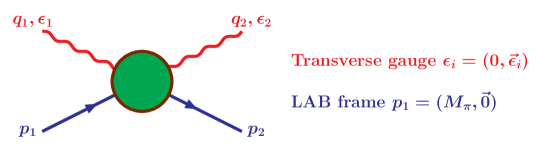
Figure 1: A schematic illustration of Compton scattering by a pion.

Expanding the Compton scattering amplitude in small photon momenta and energies, one finds

$$T_{\gamma\pi^{+}\to\gamma\pi^{+}} = \underbrace{-2\,e^{2}\,\vec{\epsilon}_{1}\cdot\vec{\epsilon}_{2}}_{\mbox{\small\bf Born term}}$$ (5)

$$+ 8\,\pi\,M_{\pi}\underbrace{\Big{\{}\alpha_{\pi}\,\omega_{1}\omega_{2}\,\vec{\epsilon}_{1}\cdot\vec{\epsilon}_{2}+\beta_{\pi}\,(\vec{\epsilon}_{1}\times\vec{q}_{1})\cdot(\vec{\epsilon}_{2}\times\vec{q}_{2})\Big{\}}}_{\mbox{\small\bf el-mag polarizabilities}}+\ldots$$

It is convenient to use the linear combinations of the electric and magnetic polarizabilities: $(\alpha-\beta)_{\pi}$ and $(\alpha+\beta)_{\pi}$ which are obtained from the helicity flip and helicity non-flip amplitudes, respectively.

As follows from the definition, the dipole pion polarizabilities are proportional to $\alpha_{\pi}(\beta_{\pi})\sim\frac{\alpha}{M_{\pi}}\frac{1}{\Lambda^{2}}\approx 4\times 10^{-4}\,{\rm fm}^{3}$ where the hadronic scale $\Lambda\sim 4\pi F_{\pi}\sim 1\,{\rm GeV}$ was used. Then a natural choice of units for the polarizabilities is $10^{-4}\,{\rm fm}^{3}$.

3 Effective Lagrangian

We consider an effective Lagrangian of QCD with two flavors in the isospin symmetry limit $m_{u}=m_{d}=\hat{m}$. At next-to-next-to-leading order (NNLO), one has [2]

$${\mathcal{L}}_{\rm eff}={\mathcal{L}}_{2}+{\mathcal{L}}_{4}+{\mathcal{L}}_{6}\,.$$ (6)

The subscripts refer to the chiral order. The expression for ${\mathcal{L}}_{2}$ is

$${\mathcal{L}}_{\,2} = \frac{F^{2}}{4}\langle D_{\mu}U\,D^{\mu}U^{\dagger}+M^{2}(U+U^{\dagger})\rangle\,,$$

$$D_{\mu}U = \partial_{\mu}U-i(QU-UQ)A_{\mu}\,,\,\ Q=\frac{e}{2}{\rm diag}(1,-1)\,,$$ (7)

where $e$ is the electric charge, and $A_{\mu}$ denotes the electromagnetic field. The quantity $F$ denotes the pion decay constant in the chiral limit, and $M^{2}$ is the leading term in the quark mass expansion of the pion (mass)², $M_{\pi}^{2}=M^{2}(1+O(\hat{m}))$. Further, the brackets $\langle\ldots\rangle$ denote a trace in flavor space. In Eq. (3), we have retained only the terms relevant for the present application, i.e., we have dropped additional external fields. We choose the unitary $2\times 2$ matrix $U$ in the form

$$U = \sigma+i\,\pi/F\,,\hskip 8.5359pt\sigma^{2}+\frac{\pi^{2}}{F^{2}}={\mathbf{1}}_{2\times 2}\,,\hskip 8.5359pt\pi=\left(\mbox{$\begin{array}[]{cc}\pi^{0}&\sqrt{2}\,\pi^{+}\\ \sqrt{2}\,\pi^{-}&-\pi^{0}\end{array}$}\right)\;.$$ (10)

The Lagrangian at NLO has the structure [2]

$${\mathcal{L}}_{4}=\sum_{i=1}^{7}l_{i}K_{i}+\sum_{i=1}^{3}h_{i}\bar{K}_{i}=\frac{l_{1}}{4}\langle D_{\mu}U\,D^{\mu}U^{\dagger}\rangle^{2}+\cdots\,,$$ (11)

where $l_{i},h_{i}$ denote low-energy couplings, not fixed by chiral symmetry. At NNLO, one has [31, 32, 30]

$${\mathcal{L}}_{6}=\sum_{i=1}^{57}c_{i}P_{i}\,.$$ (12)

As was shown in Ref. [40] the number of operators $P_{i}$ can be reduced by at least one from 57 to 56. For the explicit expressions of the polynomials $K_{i},\bar{K}_{i}$ and $P_{i}$, we refer the reader to Refs. [2, 31, 32, 30]. The vertices relevant for $\gamma\gamma\rightarrow\pi^{+}\pi^{-}$ involve $l_{1},\ldots,l_{6}$ from ${\mathcal{L}}_{4}$ and several $c_{i}$’s from ${\mathcal{L}}_{6}$, see below.

The couplings $l_{i}$ and $c_{i}$ absorb the divergences at order $p^{4}$ and $p^{6}$, respectively,

$$l_{i} = (\mu\,c)^{d-4}\left\{l_{i}^{r}(\mu,d)+\gamma_{i}\,\Lambda\right\}\,,$$

$$c_{i} = \frac{(\mu\,c)^{2(d-4)}}{F^{2}}\left\{c_{i}^{r}(\mu,d)-\gamma_{i}^{(2)}\,\Lambda^{2}-(\gamma_{i}^{(1)}+\gamma_{i}^{(L)}(\mu,d))\,\Lambda\right\}\,,$$

$$\Lambda = \frac{1}{16\,\pi^{2}(d-4)}\,,\,\ln c=-\frac{1}{2}\left\{\ln 4\pi+\Gamma^{\prime}(1)+1\right\}\,.$$ (13)

The physical couplings are $l_{i}^{r}(\mu,4)$ and $c_{i}^{r}(\mu,4)$, denoted by $l_{i}^{r},c_{i}^{r}$ in the following. The coefficients $\gamma_{i}$ are given in [2], and $\gamma_{i}^{(1,2,L)}$ are tabulated in [32]. We shall use the scale independent quantities $\bar{l}_{i}$ introduced in [2],

$$l_{i}^{r} = \frac{\gamma_{i}}{32\pi^{2}}\,({\bar{l}}_{i}+l)\,,$$ (14)

where the chiral logarithm is $l=\ln(M^{2}_{\pi}/\mu^{2})$. We shall use [8]

$$\bar{l}_{1}=-0.4\pm 0.6\,,\,\,\bar{l}_{2}=4.3\pm 0.1\,,\,\,\bar{l}_{3}=2.9\pm 2.4\,,\,\,\bar{l}_{4}=4.4\pm 0.2\,,$$ (15)

and

$$\bar{l}_{\Delta}\doteq\bar{l}_{6}-\bar{l}_{5}=3.0\pm 0.3$$ (16)

obtained from radiative pion decay to two loop accuracy [9, 41].

The constants $c_{i}^{r}$ occur in the combinations

$$a_{1}^{r} = -4096\pi^{4}\left(6\,c_{6}^{r}+c_{29}^{r}-c_{30}^{r}-3\,c_{34}^{r}+c_{35}^{r}+2\,c_{46}^{r}-4\,c_{47}^{r}+c_{50}^{r}\right)\,,$$

$$a_{2}^{r} = 256\pi^{4}\left(8\,c_{29}^{r}-8\,c_{30}^{r}+c_{31}^{r}+c_{32}^{r}-2\,c_{33}^{r}+4\,c_{44}^{r}+8\,c_{50}^{r}-4\,c_{51}^{r}\right)\,,$$

$$b^{r} = -128\pi^{4}\left(c_{31}^{r}+c_{32}^{r}-2\,c_{33}^{r}-4\,c_{44}^{r}\right)\,.$$

As follows from the resonance exchange model  [7]

$$\Big{(}a_{1}^{r},a_{2}^{r},b^{r}\Big{)}=\Big{(}-3.2,0.7,0.4\Big{)}\qquad[{\mbox{ present work }}]\,.$$ (17)

The values of these constants were obtained in the ENJL model [42] $(a_{1}^{r},a_{2}^{r},b^{r})=(-8.7,5.9,0.38)$ One can see that only $b^{r}$ agrees in the two approaches. We shall use $b^{r}=0.4\pm 0.4$. The combinations $(\alpha\pm\beta)_{\pi^{\pm}}$ are independent of $a_{2}^{r}$ and are determined precisely by the chiral expansion to two loops, once $a_{1}^{r}$ is fixed. We will then simply display this quantity as a function of $a_{1}^{r}$ - the result turns out to be rather independent of its exact value.

4 Evaluation of the diagrams

The lowest-order contributions to the scattering amplitude are described by tree- and one-loop diagrams. These contributions were calculated in [26]. The two-loop diagrams are displayed in Figs. 2, 4 and 5. The two-loop diagrams in Fig. 2 may be generated according to the scheme indicated in Fig. 3, where the filled in blob denotes the $d$-dimensional elastic $\pi\pi$-scattering amplitude at one-loop accuracy, with two pions off-shell.

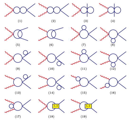
Figure 2: A set of two-loop diagrams generated by ${\mathcal{L}}_{2}$ and one-loop diagrams generated by ${{\mathcal{L}}_{4}.}$

The diagrams shown in Fig. 4 may be reduced to tree-diagrams by using Ward identities. They sum up to the expression

$$2\,Z_{\pi}\,g^{\mu\nu}-\left\{(2p_{1}-q_{1})^{\mu}(2p_{2}-q_{2})^{\nu}\left[\frac{1}{M^{2}_{\pi}-t}-Z_{\pi}R(t)\right]+{\rm crossed}\right\},$$ (18)

where $Z_{\pi}$ is the pion renormalization constant. The function $R(t)$ starts at order $1/F^{4}_{\pi}$ and can be obtained from the full pion propagator.

Two further diagrams are displayed in Fig. 5. The first one - called “acnode” in the literature - may again be evaluated by use of a dispersion relation, see [4] . The second one is trivial to evaluate, because it is a product of one-loop diagrams. The remaining diagrams at order $p^{6}$ are shown in Fig. 6.

The evaluation of the diagrams was done in the manner described in [4, 33] by invoking FORM [43]. In particular, we have verified that the counterterms from the Lagrangian ${\mathcal{L}}_{6}$ [32] remove all ultraviolet divergences, which is a very non-trivial check on our calculation. Furthermore, we have checked that the (ultra-violet finite) amplitude so obtained is scale independent.

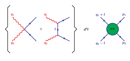
Figure 3: Construction scheme for the diagrams in Fig. 2.

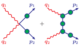
Figure 4: A class of one-particle reducible diagrams. The filled in circles summarize self-energy and vertex corrections.

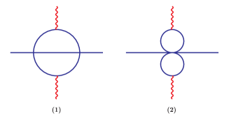
Figure 5: Acnode and butterfly diagrams.

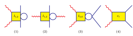
Figure 6: The remaining diagrams at order $p^{6}$: one-loop graphs generated by ${\mathcal{L}}_{4}$, and counterterm contributions from ${\mathcal{L}}_{6}$.

5 Chiral expansion for pion polarizabilities

Using the same notation as in [7], we find for the dipole polarizabilities

$$(\alpha\pm\beta)_{\pi^{+}}=\frac{\alpha}{16\,\pi^{2}\,F_{\pi}^{2}\,M_{\pi}}\,\left\{c_{1\pm}+\frac{M_{\pi}^{2}\,d_{1\pm}}{16\,\pi^{2}\,F_{\pi}^{2}}+O(M^{4}_{\pi})\right\}\,,$$ (19)

where

$$c_{1+} = 0,\qquad c_{1-}=\frac{2}{3}\,\bar{l}_{\Delta}\,,$$

$$d_{1+} = 8\,b^{r}-\frac{4}{9}\left\{l\,\left(l+\frac{1}{2}\,\bar{l}_{1}+\frac{3}{2}\,\bar{l}_{2}\right)-\frac{53}{24}\,l+\frac{1}{2}\,\bar{l}_{1}+\frac{3}{2}\,\bar{l}_{2}+\frac{91}{72}+\Delta_{+}\right\}\;\;,$$

$$d_{1-} = a_{1}^{r}+8\,b^{r}-\frac{4}{3}\left\{l\left(\bar{l}_{1}-\bar{l}_{2}+\bar{l}_{\Delta}-\frac{65}{12}\right)-\frac{1}{3}\,\bar{l}_{1}-\frac{1}{3}\,\bar{l}_{2}+\frac{1}{4}\,\bar{l}_{3}-\bar{l}_{\Delta}\bar{l}_{4}\right.$$ (20)

$$\left.+\frac{187}{108}+\Delta_{-}\right\}\,,$$

with

$$\Delta_{+} = \frac{8105}{576}-\frac{135}{64}\,\pi^{2}\,,\qquad\Delta_{-}=\frac{41}{432}-\frac{53}{64}\,\pi^{2}\,.$$ (21)

It would be interesting to numerically compare the values of $\Delta_{\pm}$ given by Eq. (21) with those obtained in Refs. [7]. One has

$$\Delta_{+}=\left\{\begin{array}[]{l}-6.75\qquad\text{our}\\ -8.69\qquad\text{Burgi}\end{array}\right.\qquad\Delta_{-}=\left\{\begin{array}[]{l}-8.08\qquad\text{our}\\ -8.73\qquad\text{Burgi}\end{array}\right.$$

The results for the polarizabilities evaluated with the central values for the LECs in Eqs. (15)-(17) are shown in Table 5.

Central values of polarizabilities in units of $10^{-4}\,{\rm fm}^{3}$. to one loop to two-loops $(\alpha-\beta)_{\pi^{+}}$   $6.0$   $5.7$ $(\alpha+\beta)_{\pi^{+}}$   $0$   $0.16$

The uncertainty in the prediction for the polarizability has two sources. First, the low-energy constants are not known precisely. Second, we are dealing here with an expansion in powers of the momenta and of the quark masses up to and including terms of order $p^{6}$. The discussion of estimating uncertainties may be found in our paper [5]. It was shown that the value for the dipole polarizability $(\alpha-\beta)_{\pi^{\pm}}$ is rather reliable - there is no sign of any large, uncontrolled correction to the two-loop result. The maximum deviation $1.0$ from the central value $5.7$ has been used as the final theoretical uncertainty for the dipole polarizability:

$$(\alpha-\beta)_{\pi^{\pm}}=(5.7\pm 1.0)\times 10^{-4}\,{\rm fm}^{3}\,.$$ (22)

The chiral expansion for the combination $(\alpha+\beta)_{\pi^{\pm}}$ starts out at order $p^{6}$ so we have determined only its leading order term.

6 Experimental information

There are three types of experiments aiming to measure the pion polarizabilities:

• The scattering of high energy pions off the Coulomb field of heavy nucleus using the Primakoff effect

• Radiative pion photoproduction from the proton

• Pion pair production in photon-photon collisions

Schematically, they are shown in Fig. 7.

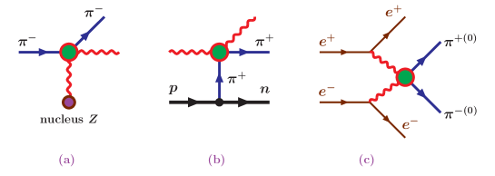
Figure 7: Schematic images of the available experiments.

The possibility to measure the pion polarizability via the Primakoff reaction was proposed in the early 1980s in [44]. The measurement of the pion-photon Compton scattering amplitude by using the Primakoff effect was performed in an experiment at Serpukhov [45] , but the small data sample led to only an imprecise value for the polarizability of $\alpha_{\pi}=(6.8\pm 1.4_{\rm stat}\pm 1.2_{\rm syst})\times 10^{-4}\,{\rm fm}^{3}$. Low statistics made it difficult to evaluate the systematic uncertainty.

COMPASS has now achieved a modern Primakoff experiment, using a 190 GeV pion beam from the Super Proton Synchrotron at CERN directed at a nickel target. It is important that COMPASS was also able to use a muon, which is point-like particle, to calibrate the experiment. The Compton $\pi^{-}\gamma\to\pi^{-}\gamma$ scattering is extracted from the reaction $\pi^{-}\,Ni\to\pi^{-}\gamma\,Ni$ by selecting events from the Coulomb peak at small momentum transfer $Q^{2}<0.0015$ GeV². From the analysis of a sample of 63,000 events, the collaboration obtained a value of the pion electric polarizability of [12] $\alpha_{\pi}=(2.0\pm 0.6_{\rm stat}\pm 0.7_{\rm syst})\times 10^{-4}\,{\rm fm}^{3}$ under assumption $(\alpha+\beta)_{\pi}=0$.

The cross section for the radiative pion photoproduction $\gamma p\to\gamma\pi^{+}n$ has been measured at the Lebedev Institute [46]. By using an extrapolation to the pion pole in the unphysical region the value of the electric polarizability was obtained $\alpha_{\pi^{+}}=-\beta_{\pi^{+}}=(20\pm 12)\times 10^{-4}\,{\rm fm}^{3}$. Similar experiment was performed at the Mainz Microtron MAMI [10] but the pion polarizability has been extracted by a comparison of the data with the predictions of two different models yielding the value $(\alpha-\beta)_{\pi^{+}}=(11.6\pm 1.5_{\rm stat}\pm 3.0_{\rm syst}\pm 0.5_{\rm mod})\times 10^{-4}\,{\rm fm}^{3}$.

Another possibility to obtain the value for the pion polarizability is to extrapolate the data from the pion pair production in photon-photon collisions $\gamma\gamma\to\pi\pi$ to the region of the Compton scattering threshold by using crossing symmetry and analyticity. Normally, the procedure involves the construction of the dispersion relations with one or two subtractions. The most recent analysis preformed in [24] produced the value $(\alpha-\beta)_{\pi^{\pm}}=13.0^{+2.6}_{-1.9}\times 10^{-4}\,{\rm fm}^{3}$ which is close to the MAMI data. There are plenty of previous studies in this direction which give quite a broad region for the value of the pion polarizability. The available experimental information is shown in Table 6.

Experimental information on $(\alpha-\beta)_{\pi^{\pm}}$, in units of $10^{-4}\,{\rm fm}^{3}$. We indicate the reaction and data used. In [52] , [47] and [12] $\alpha_{\pi}$ was determined, using as a constraint $\alpha_{\pi}=-\beta_{\pi}$. To obtain $(\alpha-\beta)_{\pi^{\pm}}$, we multiplied the results by a factor of 2.     Experiments $(\alpha-\beta)_{\pi^{\pm}}$ $\pi^{-}Z\to\gamma\pi^{-}Z$ Serpukhov (1983) [45] $15.6\pm 6.4_{\,\rm stat}\pm 4.4_{\,\rm syst}$ $\gamma p\to\gamma\pi^{+}n$ Lebedev Inst. (1984) [46] $40\pm 24$ D. Babusci et al. (1992)  [47] $\gamma\gamma\to\pi^{+}\pi^{-}$ PLUTO  [48] $38.2\pm 9.6\pm 11.4$ DM 1  [49] $34.4\pm 9.2$ DM 2  [50] $52.6\pm 14.8$ MARK II  [51] $4.4\pm 3.2$ J.F. Donoghue, B. Holstein (1993)  [52] $5.4$ $\gamma\gamma\to\pi^{+}\pi^{-}$ MARK II [51] A. Kaloshin, V. Serebryakov (1994)  [53] $5.25\pm 0.95$ $\gamma\gamma\to\pi^{+}\pi^{-}$ MARK II  [51] Crystal Ball Coll. [54] $\gamma p\to\gamma\pi^{+}n$ Mainz (2005) [10] $11.6\pm 1.5_{\,\rm stat}\pm 3.0_{\,\rm syst}\pm 0.5_{\,\rm mod}$ L. Fil’kov, V. Kashevarov (2005)  [24] $13.0^{+2.6}_{-1.9}$ $\gamma\gamma\to\pi^{+}\pi^{-}$ MARK II  [51] , TPC/2$\gamma$ [55] ,  CELLO  [56] , VENUS  [57] , ALEPH  [58] ,  BELLE [59] $\pi^{-}Z\to\gamma\pi^{-}Z$ COMPASS (2015) [12] $4.0\pm 1.2_{\,\rm stat}\pm 1.4_{\,\rm syst}$

Acknowledgments

I would like to thank Juerg Gasser and Mikko Sainio for their collaboration in which the results for pion polarizabilities at two-loop level accuracy were obtained. It has been a pleasure to discuss many points of this subject with L. V. Fil’kov, S. B. Gerasimov, A. G. Olshevski, V. A. Petrunkin and M. K. Volkov. I am also grateful to Stanislav Dubnička and Zuzana Dubničková for inviting me to give a talk at the conference “Hadron Structure’15” .

References

- [1] S. Weinberg, Physica A 96, 327 (1979).
- [2] J. Gasser and H. Leutwyler, Ann. Phys. 158, 142 (1984).
- [3] J. Gasser and H. Leutwyler, Nucl. Phys. B 250, 465 (1985).
-
[4]
J. Gasser, M. A. Ivanov and M. E. Sainio,
Nucl. Phys. B 728, 31 (2005)
[hep-ph/0506265]. -
[5]
J. Gasser, M. A. Ivanov and M. E. Sainio,
Nucl. Phys. B 745, 84 (2006)
[hep-ph/0602234]. -
[6]
S. Bellucci, J. Gasser and M. E. Sainio,
Nucl. Phys. B 423, 80 (1994)
[Erratum-ibid. B 431, 413 (1994)] [arXiv:hep-ph/9401206]. -
[7]
U. Burgi,
Nucl. Phys. B 479, 392 (1996)
[arXiv:hep-ph/9602429];
U. Burgi, Phys. Lett. B 377, 147 (1996) [arXiv:hep-ph/9602421]. -
[8]
G. Colangelo, J. Gasser and H. Leutwyler,
Nucl. Phys. B 603, 125 (2001)
[arXiv:hep-ph/0103088]. - [9] J. Bijnens and P. Talavera, Nucl. Phys. B 489, 387 (1997) [arXiv:hep-ph/9610269].
- [10] J. Ahrens et al., Eur. Phys. J. A 23, 113 (2005) [arXiv:nucl-ex/0407011].
- [11] S. Scherer, Eur. Phys. J. A 28, 59 (2006) [hep-ph/0512291].
- [12] COMPASS Collab. (C. Adolph et al. ), Phys. Rev. Lett. 114, 062002 (2015) [arXiv:1405.6377 [hep-ex]].
- [13] A. Klein, Phys. Rev. 99, 998 (1955).
- [14] A.M. Baldin, Nucl. Phys. 18, 310 (1960).
- [15] V.A. Petrunkin, JETP 13, 804 (1961).
- [16] V. A. Petrunkin, Nucl. Phys. 55, 197 (1964).
-
[17]
M. V. Terentev,
Sov. J. Nucl. Phys. 16, 87 (1973)
[Yad. Fiz. 16, 162 (1972)];
M. V. Terentev, Sov. J. Nucl. Phys. 19, 664 (1974) [Yad. Fiz. 19, 1298 (1974)]. - [18] M. Bychkov et al., Phys. Rev. Lett. 103, 051802 (2009) [arXiv:0804.1815 [hep-ex]].
- [19] A. I. L’vov, Sov. J. Nucl. Phys. 34, 289 (1981) [Yad. Fiz. 34, 522 (1981)].
-
[20]
M. K. Volkov and D. Ebert,
Sov. J. Nucl. Phys. 34, 104 (1981)
[Yad. Fiz. 34, 182 (1981)]; Phys. Lett. B 101, 252 (1981). -
[21]
M. K. Volkov and A. A. Osipov,
Sov. J. Nucl. Phys. 41, 659 (1985)
Yad. Fiz. 41, 1027 (1985). - [22] V. Bernard, B. Hiller and W. Weise, Phys. Lett. B 205, 16 (1988).
- [23] L. V. Filkov, I. Guiasu and E. E. Radescu, Phys. Rev. D 26, 3146 (1982).
- [24] L. V. Fil’kov and V. L. Kashevarov, Phys. Rev. C 73, 035210 (2006) [nucl-th/0512047].
- [25] M. A. Ivanov and T. Mizutani, Phys. Rev. D 45, 1580 (1992).
- [26] J. Bijnens and F. Cornet, Nucl.Phys. B 296, 557 (1988).
- [27] J. F. Donoghue and B. R. Holstein, Phys. Rev. D 40, 2378 (1989).
- [28] T. Das, V. S. Mathur and S. Okubo, Phys. Rev. Lett. 19, 859 (1967).
- [29] A. E. Dorokhov and W. Broniowski, Eur. Phys. J. C 32, 79 (2003) [hep-ph/0305037].
- [30] H. W. Fearing and S. Scherer, Phys. Rev. D 53, 315 (1996) [arXiv:hep-ph/9408346].
-
[31]
J. Bijnens, G. Colangelo and G. Ecker,
JHEP 9902, 020 (1999)
[arXiv:hep-ph/9902437]. -
[32]
J. Bijnens, G. Colangelo and G. Ecker,
Ann. Phys. 280, 100 (2000)
[arXiv:hep-ph/9907333]. - [33] J. Gasser and M. E. Sainio, Eur. Phys. J. C 6, 297 (1999) [arXiv:hep-ph/9803251].
-
[34]
V. A. Petrunkin,
Sov. J. Part. Nucl. 12, 278 (1981)
[ Fiz. Elem. Chast. Atom. Yadra 12, 692 (1981)]. - [35] B. R. Holstein and S. Scherer, Ann. Rev. Nucl. Part. Sci. 64, 51 (2014) [arXiv:1401.0140 [hep-ph]].
-
[36]
E. V. Luschevskaya, O. E. Solovjeva, O. A. Kochetkov and O. V. Teryaev,
Nucl. Phys. B 898, 627 (2015) [arXiv:1411.4284 [hep-lat]]. - [37] M. Lujan, A. Alexandru, W. Freeman and F. Lee, Phys. Rev. D 89, 074506 (2014) [arXiv:1402.3025 [hep-lat]].
- [38] W. Detmold, B. C. Tiburzi and A. Walker-Loud, Phys. Rev. D 79, 094505 (2009) [arXiv:0904.1586 [hep-lat]].
-
[39]
J. Hu, F. J. Jiang and B. C. Tiburzi,
Phys. Rev. D 77, 014502 (2008)
[arXiv:0709.1955 [hep-lat]]. - [40] C. Haefeli, M. A. Ivanov, M. Schmid and G. Ecker, “On the mesonic Lagrangian of order in chiral SU(2),” arXiv:0705.0576 [hep-ph].
-
[41]
C. Q. Geng, I. L. Ho and T. H. Wu,
Nucl. Phys. B 684, 281 (2004)
[arXiv:hep-ph/0306165]. - [42] J. Bijnens and J. Prades, Nucl. Phys. B 490, 239 (1997) [arXiv:hep-ph/9610360].
- [43] J. A. M. Vermaseren, “New features of FORM,” arXiv:math-ph/0010025.
-
[44]
A. S. Galperin, G. Mitselmakher, A. G. Olszewski and V. N. Pervushin,
Yad. Fiz. 32, 1053 (1980). -
[45]
Y. M. Antipov et al.,
Z. Phys. C 26 (1985) 495;
Y. M. Antipov et al., Phys. Lett. B 121 (1983) 445. - [46] T. A. Aibergenov et al., Czech. J. Phys. B 36, 948 (1986).
- [47] D. Babusci, S. Bellucci, G. Giordano, G. Matone, A. M. Sandorfi and M. A. Moinester, Phys. Lett. B 277, 158 (1992).
- [48] PLUTO Collab. (C. Berger et al.), Z. Phys. C 26, 199 (1984).
- [49] DM1-DM2 Collab. (A. Courau et al.), Nucl. Phys. B 271, 1 (1986).
-
[50]
DM1-DM2 Collab. (Z. Ajaltouni et al.),
Phys. Lett. B 194, 573 (1987)
[Erratum-ibid. Phys. Lett. B 197, 565 (1987)]. - [51] MARK-II Collab. (J. Boyer et al.), Phys. Rev. D 42, 1350 (1990).
-
[52]
J. F. Donoghue and B. R. Holstein,
Phys. Rev. D 48, 137 (1993)
[arXiv:hep-ph/9302203]. -
[53]
A. E. Kaloshin and V. V. Serebryakov,
Z. Phys. C 64, 689 (1994)
[arXiv:hep-ph/9306224]. - [54] Crystal Ball Collab. (H. Marsiske et al.), Phys. Rev. D 41, 3324 (1990).
- [55] TPC/Two-Gamma Collab. (H. Aihara et al.) , Phys. Rev. Lett. 57, 404 (1986).
- [56] CELLO Collab. (H. J. Behrend et al.), Z. Phys. C 56, 381 (1992).
- [57] VENUS Collab. (F. Yabuki et al.), J. Phys. Soc. Jap. 64, 435 (1995).
- [58] ALEPH Collab. (A. Heister et al.), Phys. Lett. B 569, 140 (2003).
-
[59]
BELLE Collab. (H. Nakazawa et al.),
Phys. Lett. B 615, 39 (2005)
[arXiv:hep-ex/0412058].