Spontaneous charge carrier localization in extended one-dimensional systems

Abstract

Charge carrier localization in extended atomic systems has been described previously as being driven by disorder, point defects or distortions of the ionic lattice. Here we show for the first time by means of first-principles computations that charge carriers can spontaneously localize due to a purely electronic effect in otherwise perfectly ordered structures. Optimally-tuned range-separated density functional theory and many-body perturbation calculations within the GW approximation reveal that in trans-polyacetylene and polythiophene the hole density localizes on a length scale of several nanometers. This is due to exchange-induced translational symmetry breaking of the charge density. Ionization potentials, optical absorption peaks, excitonic binding energies and the optimally-tuned range parameter itself all become independent of polymer length as it exceeds the critical localization scale. Moreover, lattice disorder and the formation of a polaron result from the charge localization in contrast to the traditional view that lattice distortions precede charge localization. Our results can explain experimental findings that polarons in conjugated polymers form instantaneously after exposure to ultrafast light pulses.

Spatial localization in extended systems has been a central topic in physics, since the pioneering work of Anderson Anderson (1958) and Mott Mott (1968), and more recently in the context of many-body localization Basko et al. (2006). It also forms an important theme in materials science of extended conjugated systems where the dynamics of charges carrier are described in terms of localized polarons. Friend et al. (1999); Brandes and Kettemann (2003); Scholes and Rumbles (2006); Johns et al. (2010); McMahon and Troisi (2010); Lannoo (2012); Noriega et al. (2013). One way to identify charge localization is through the dependence of its energy (e.g., ionization potential or electron affinity) on the system size $L$. In 1D systems, if the charge remains delocalized, then according to a simple non-interacting picture, its energy converges to the bulk limit as $1/L^{\alpha}$ with $\alpha=1$ for a metal or $\alpha=2$ otherwise. However, if the energy becomes independent of $L$ for $L>\ell_{c}$, it could be due to charge localization within a critical length scale $\ell_{c}$.

Charge localization in conjugated systems can occur in several ways: Attachment by point defects Lannoo (2012), lattice disorder effects Brandes and Kettemann (2003); Noriega et al. (2013), and formation of self-bound charged polarons and neutral solitons by local distortion of the nuclear lattice Kurlancheek et al. (2012); Salzner (2014); Körzdörfer and Brédas (2014); Köhler and Bässler (2015). However, it still remains an open question whether localization can occur in disorder-free transitionally invariant systems. This question has received much attention recently in the context of many-body localization Yao et al. (2014); De Roeck and Huveneers (2014); Hickey et al. (2014); Schiulaz et al. (2015).

In this letter we provide first-principles computational evidence for a new mechanism of localization in 1D conjugated systems, in which the electrons form their own nucleation center without the need to introduce disorder into the Hamiltonian. This challenges the widely accepted picture in which the electronic eigenstates localize only after coupling with the lattice distortion Holstein (1959). To illustrate this mechanism, we study the electronic structure and the charge distribution in large one-dimensional systems with ideal (ordered) geometries. We focus on two representative conjugated polymers, trans-polyacetylene (tPA) and polythiophene (PT), with increasing lengths $L=M\ell_{1}$ up to $M=70$ and $M=20$, respectively ($\ell_{1}$ is the length of the repeat unit). Besides their practical significance Scholes and Rumbles (2006), they also exhibit interesting physical phenomena, in which polarons, bipolarons and solitons affect charge mobility and localization Puschnig and Ambrosch-Draxl (2003); Friend et al. (1999); Nayyar et al. (2011); Hoffmann et al. (2013); Salzner (2014).

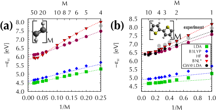
Figure 1: Ionization potentials (estimated using highest occupied eigen-energies $\varepsilon_{H}$) for (a) trans-polyacetylene and (b) polythiophene shown against the inverse number of repeat units $M$ in the respective polymer. The repeat unit for each polymer is illustrated in the corresponding insets (C, H and S are shown by black, white and yellow spheres, respectively). Results obtained from different computational approaches are indicated by colors and labelled in the figure. Experimental data for the ionization potentials (gray circles) were taken from Refs. 23; 24; 25 and references therein. The dashed lines represent a numerical fit to $-\varepsilon_{H}\left(M\right)=-\varepsilon_{H}\left(\infty\right)+\frac{\Delta\varepsilon}{M}$ for LDA and B3LYP ($\varepsilon_{H}\left(\infty\right)$ and $\Delta\varepsilon$ are fitting parameters) and to $-\varepsilon_{H}\left(M\right)=-\varepsilon_{H}\left(\infty\right)+\Delta\varepsilon\exp\left(-\sqrt{M/M_{0}}\right)$ for HF, BNL*, and GW.

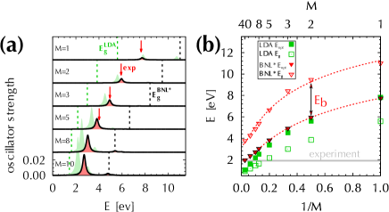
Figure 2: (a) Calculated optical spectra for selected tPA polymers of various lengths (numbers of repeat units $M$). All calculations were performed with the cc-pvTZ basis set using TDDFT within the BNL* functional (solid black line with red fill) and LDA functional (green filled curve). The fundamental band gaps are shown by dashed vertical lines in corresponding colors. Red arrows indicate experimental absorption peak positions (Refs. 26; 27; 28; 29 and references therein). (b) Position of the first maxima of the absorption $E_{opt}$ and the fundamental band gap $E_{g}$ obtained with BNL* and LDA functionals as function of inverse number of repeat units. Results for the two longest polymers were calculated using the 3-21G basis set, other results are obtained using cc-pvTZ. The exciton binding energy is the difference between $E_{g}$ and the peak maximum is illustrated by an arrow. The horizontal full line represents the experimental energy of the maximum absorption for the infinite system (1.9 eV) Feldblum et al. (1982).

In Fig. 1 we plot the ionization potentials (IPs) for both the tPA ( panel a) and PT (panel b) polymers as a function of the number of repeat units, $M$. To illustrate the effect of localization we focus on the ionization potential representing the energy of positive charge carrier (hole) rather than on the electron affinity representing the energy of negative charge carrier (electron), since we find the former to localize on shorter length scales (see below). Several levels of theory are used: Hartree-Fock (HF) theory, density functional theory (DFT) within the local density approximation (LDA) Perdew and Wang (1992), the optimally-tuned BNL* Baer and Neuhauser (2005); Baer et al. (2010); Kronik et al. (2012) range-separated hybrid functional Savin and Flad (1995), and the B3LYP Becke (1993) approximation, and, finally, the $\mbox{G}_{0}\mbox{W}_{0}$ many-body perturbation technique Hybertsen and Louie (1986) (on top of of LDA implemented using stochastic DFT Baer et al. (2013)) within the stochastic formulation (sGW) Neuhauser et al. (2014). The LDA and to some extent the B3LYP lack sufficient exact exchange while HF lacks correlations and screening effects. BNL* provide a systematic description of correlations and exact exchange through the process of optimal tuning Livshits and Baer (2007). $\mbox{G}_{0}\mbox{W}_{0}$ is based on many-body perturbation theory and includes exchange, correlation and screening effects Hybertsen and Louie (1986).

The LDA and B3LYP computations yield IPs that are considerably smaller than the experimental values, consistent with previous computational studies on shorter polymer chains Salzner (2010); Salzner and Aydin (2011) and with general theoretical arguments Salzner and Baer (2009); Stein et al. (2012). These IP values drop to their bulk limit ($I_{\infty}^{tPA}=4.4$ eV for tPA and $I_{\infty}^{PT}=4.6$ eV for PT) asymptotically linearly as $M^{-1}$ for the range of sizes studied (they do not fit the purely non-interacting asymptotic dependence of $M^{-2}$). In contrast, HF IPs are significantly closer to the experimental values, deviating by less than $0.4$ eV. The HF IPs also initially drop as polymer size increases but for a polymer of length exceeding a critical value, they quickly converge to an asymptotic value, hinting at localization of the hole. The asymptotic HF IPs and HF critical length scale are $I_{\infty}^{tPA}=6.1$ eV and $\ell_{c}^{tPA}=4.9$ nm and $I_{\infty}^{PT}=6.4$ eV and $\ell_{c}^{PT}=3.1$ nm (see Supplementary Material for the approach used to determine these quantities). The computational IPs of BNL* and the sGW are in even better agreement with the available experimental data than those of HF. They too show a localization transition with $I_{\infty}^{tPA}=5.9$ eV and $\ell_{c}^{tPA}=7.9$ nm for tPA and $I_{\infty}^{PT}=6.4-6.5$ eV and $\ell_{c}^{PT}=4.2-4.3$ nm for PT. Using the results for intermediate polymers (which do not exhibit localization yet) we can linearly extrapolate to the limit $M\to\infty$ and estimate the value of ionization potential if no localization occurs; this yields IP values smaller by $\approx 0.5$ eV which can be viewed as the energy of spontaneous localization. While the asymptotic values of the ionization potentials predicted by HF, BNL* and sGW are similar, the BNL* and sGW critical length scales $\ell_{c}$ are larger than those predicted by HF. This result is consistent with the tendency of HF to over-localize holes in finite systems Mori-Sánchez et al. (2008); Livshits and Baer (2008).

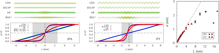
Figure 3: Left panels: The hole densities (top two panels), $\Delta n\left(\mathbf{r}\right)$, for the corresponding labelled methods in long strands of $M=50$ repeat tPA units (left) and $M=20$ repeat PT units (right). The hole is shown as a yellow (aqua) 0.00025$a_{0}^{-3}$ (-0.00025$a_{0}^{-3}$) density isosurface. In the two bottom left panels we plot the cumulative density, $\rho\left(z\right)$, for different functionals. The cumulative curve for a shorter tPA polymer with $M=40$ (black line) is practically indistinguishable from $M=50$. Gray areas in the plots show the value of the second cumulant ($\sigma$) for the corresponding BNL* hole density, which are plotted in the right panel for different polymer lengths. The dashed straight line in the right panel is the fully delocalized result ($\sigma=L/\sqrt{12}$). Note that for the larger system we used a smaller basis (3-21G, black symbols) which closely follow the results using a larger basis (cc-pvTZ, red symbols).

To further strengthen the validity of the BNL* treatment (and indirectly the $\mbox{G}_{0}\mbox{W}_{0}$ which agrees with the BNL*), we compare its predicted optical excitations $E_{opt}$ and fundamental gaps $E_{g}=\varepsilon_{L}-\varepsilon_{H}$ in tPA to experimental results, where available McDiarmid (1976); Flicker et al. (1977); D’Amico et al. (1980); Bredas et al. (1983) (see Table II of the Supplementary material). The absorption spectra shown in the left panel of Fig. 2 were calculated using time-dependent LDA (ALDA) and BNL* (ABNL*) functionals Stein et al. (2009); Baer et al. (2010). It is seen that the ABNL* approach provides excellent agreement for the optical gaps $E_{opt}^{ABNL*}$ in comparison to experimental data. The optical gaps $E_{opt}$ are also plotted as a function of $1/M$ on the right panel of Fig. 2 and it is seen that for the largest system studied the ABNL* optical gap is in excellent agreement with the experimental value Feldblum et al. (1982); Leising (1988). This is in contrast to the ALDA results which underestimate this limit by $\approx 1$ eV, and consistently deviate from the ABNL* results as the system size increases. In the right panel of Fig. 2 we also plot the fundamental gap $E_{g}^{BNL*}$. The values of $E_{g}^{BNL*}$ for small systems yields excellent agreement with previous $\mbox{G}_{0}\mbox{W}_{0}$ results Pinheiro et al. (2015). Furthermore, $E_{g}^{BNL*}$ does not localize for the tPA lengths studied. Since, $\varepsilon_{H}^{BNL*}$ localizes within a length scale of $\ell_{c}=7.9$ nm the continued change in $E_{g}^{BNL*}$ for larger polymers must result from a continued change in the electron energy $\varepsilon_{L}^{BNL*}$. This suggests that negative added charge does not yet localize for the tPA sizes studied and may explain why the finite size gaps are larger than the $\mbox{G}_{0}\mbox{W}_{0}$ gap of 2.1 eV for $L\rightarrow\infty$ Rohlfing and Louie (1999); Puschnig and Ambrosch-Draxl (2003); Rohra et al. (2006). Note, however, that the $\mbox{G}_{0}\mbox{W}_{0}$ gaps are rather sensitive to the size of the unit cell and small changes of 0.005 nm in the position of the atoms can lead to significant fluctuation of $2.0$ to $4.2$ eV in the gaps Ferretti et al. (2012). Since there are no experimental measurements of the fundamental gap when $L\rightarrow\infty$, it still remains an open question as to the length scale at which electrons localize (as opposed to hole localization, which already occurs at the system sizes studied). To reach system sizes at which the electron localizes will probably require using a stochastic approach for BNL* Neuhauser et al. (2015). Finally, panel a of Fig. 2 shows that the exciton binding energy $E_{b}=E_{g}-E_{opt}$ is on the order of $E_{g}/2$ for the larger systems, a value typical of other 1D conjugated systems Wang et al. (2005), indicating that neutral excitations are dominated by electron-hole interactions.

Up to now we have studied localization only from the point of view of energy changes. It is instructive to also study localization in terms of the hole density, which is the difference $\Delta n\left(\mathbf{r}\right)=n^{N}\left(\mathbf{r}\right)-n^{N-1}\left(\mathbf{r}\right)$ between the ground state density of the neutral ($N$) and the ground state density of the positively charged ($N-1$) systems. For non-interacting electrons this quantity equals the density of the highest occupied eigenstate, which is not localized. However, for interacting electrons $\Delta n\left(\mathbf{r}\right)$ must be calculated as the difference of densities obtained from two separate self-consistent field DFT calculations and can thus exhibits a different behavior. We have also ascertained that the same localization pattern emerges even when an infinitesimal charge $q\to 0$ is removed, showing that localization of the hole density occurs even also in the linear response regime.

The isosurface plots of the hole densities are given in the upper left and middle panels of Fig. 3 for the various methods (excluding sGW). In the lower left and middle panels we show the cumulative hole densities $\rho\left(z\right)=\int_{-\infty}^{z}{\rm d}z^{\prime}\int_{-\infty}^{\infty}{\rm d}y^{\prime}\int_{-\infty}^{\infty}{\rm d}x^{\prime}\Delta n\left(\mathbf{r^{\prime}}\right)$. In both types of plots it is evident that LDA and B3LYP do not show localization of the hole density in any of the systems studied and in $\rho\left(z\right)$ they show a linear monotonic increase. Contrarily, the HF and BNL* charge distributions localize as observed by change of $\rho\left(z\right)$ near the center of the chain. In PT this transition in $\rho\left(z\right)$ occurs around one of the S atoms closest to the center of the polymer, due to the lack of mirror plane symmetry. For long polymers exceeding $\ell_{c}$, the BNL* hole density hardly changes as seen by the overlapping $\rho\left(z\right)$ of polymers with $M=40$ and $M=50$. This implies that the size of the hole is no longer influenced by the polymer terminal points and is thus independent of system size.

The extent of hole localization can be described by the second cumulant $\sigma=\sqrt{\int\Delta n\left(\mathbf{r}^{\prime}\right)\left(z^{\prime}-\bar{z}\right)^{2}d\mathbf{r}^{\prime}}$ (where $\bar{z}=\int\Delta n\left(\mathbf{r}^{\prime}\right)z^{\prime}d\mathbf{r}^{\prime}$). This is shown in the right panel of Fig. 3 for BNL*. For small sizes $\sigma$ increases as $L/\sqrt{12}$, consistent with a uniform hole density spread over the entire polymer. As $L$ increases beyond $\ell_{c}$, the BNL* $\sigma$ converge to an asymptotic value, $\sigma_{\infty}$, while those of LDA continue to follow the linear $L/\sqrt{12}$ law (not shown).

It is important to note that the hole density $\Delta n\left(\mathbf{r}\right)$ is dominated by the minority-spin density changes: the orbitals having the same spin as the removed electron redistribute such as to localize the hole density near the chain center. On the other hand, the majority-spin orbitals remain nearly unperturbed and thus do not contribute to $\Delta n\left(\mathbf{r}\right)$. This fact reveals that the localization is driven by attractive non-local exchange interactions existing solely between like-spin electrons. This is further supported by the fact that localization only appears in methods that account for non-local exchange (HF, BNL*, and $\mbox{G}_{0}\mbox{W}_{0}$).

One of the interesting ramifications of the IP stabilization as polymer length exceeds a critical length scale is the simultaneous stabilization of the BNL* range-separation parameter $\gamma$. This is because in the absence of hole localization the tuning criterion,Livshits and Baer (2007) $I+\varepsilon_{H}=0$ is expected to become automatically satisfied when (semi)local functionals are used in the limit of infinite system size Godby and White (1998); Öǧüt et al. (1997); Mori-Sánchez et al. (2008); Vlček et al. (2015) forcing $\gamma$ (and with it the non-local exchange part of the functional) to drop eventually to zero. In the systems studied here localization saves the day for tuning and the range parameter attains finite asymptotic values of $\gamma^{tPA}=2.7$ nm^-1 and $\gamma^{PT}=3.1$ nm^-1. The leveling of $\gamma$ with $L$ was reported for PT Körzdörfer et al. (2011), however, it was not previously clear whether $\gamma$ would level-off for tPA. It is worth pointing out that $\gamma$ does not change significantly ($<0.2\,\mbox{nm}^{-1}$) when LYP correlation is used instead of LDA in the BNL* calculation.

While HF supports partial localization, its hole density also exhibits oscillations along the entire polymer length that do not diminish with system size. These indicate a rigid shift of charge between neighboring atoms: From double to single C-C bonds in tPA and from S to nearby C atoms for PT. This is consistent with the tendency of HF to eliminate bond-length alternation in the entire tPA polymer chain Rodrigues-Monge and Larsson (1995) as shown in the left panel of Fig. 4. BNL* on the other hand eliminates the bond-length alternation only in proximity of the localized hole density (right panel of Fig. 4), consistent with a localized polaron model.

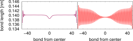
Figure 4: The C-C bond length in the charged $M=50$ tPA polymer as predicted by HF (left panel) and BNL* (right panel) obtained with the 3-21G basis set. In BNL*, a polaron appears as a reduction of the bond-length alternation, while in the region about 40 C-C bonds away from the polaron, the alternation is increased to $0.007$ nm, similar to the experimental value of $0.008\,\mbox{nm}$ for neutral chains Yannoni and Clarke (1983).

In summary, using first principles density functional theory and many-body perturbation theory, we have shown that positive charge carriers can localize in 1D conjugated polymers due to a spontaneous, purely electronic symmetry breaking transition. In this case, localization is driven by non-local exchange interactions and thus cannot occur when (semi)local density functional approximations are used. HF theory, which has non-local exchange, shows a localization transition in a relatively small length-scale but predicts complete annihilation of bond-length alternation upon ionization, irrespective of polymer length. BNL*, which through tuning includes a balanced account of local and non-local exchange effects, provides an accurate description of the optical gap in comparison to experiments and shows a localization transition with a length scale (estimated from the leveling off of the IPs) that agrees well with the sGW approach. Moreover, BNL* predicts a localized disruption of the bond-length alternation.

The localization phenomenon is driven by the same-spin attractive non-local exchange interactions and therefore, cannot be explained in terms of classical electrostatics. There is no reason to assume that the observed emergence of the localization length $\ell_{c}$ in finite systems will not readily occur also in infinite systems, where hole states near the top of the valence band are necessarily infinitely degenerate.

We thank professors Ulrike Salzner and Leeor Kronik for illuminating discussions on polymers and localization in large systems. R.B. and E.R. are supported by The Israel Science Foundation–FIRST Program (Grant No. 1700/14). V.V. is supported by Minerva Stiftung of the Max Planck Society, R.B. gratefully acknowledges support for his sabbatical visit by the Pitzer Center and the Kavli Institute of the University of California, Berkeley. D.N. and E.R. acknowledge support by the NSF, grants CHE-1112500 and CHE-1465064, respectively. This research used resources of the National Energy Research Scientific Computing Center, a DOE Office of Science User Facility supported by the Office of Science of the U.S. Department of Energy under Contract No. DE-AC02-05CH11231, and at the Leibniz Supercomputing Center of the Bavarian Academy of Sciences and the Humanities.

References

- Anderson (1958) P. W. Anderson, Phys. Rev. 109, 1492 (1958).
- Mott (1968) N. F. Mott, Rev. Mod. Phys. 40, 677 (1968).
- Basko et al. (2006) D. Basko, I. Aleiner, and B. Altshuler, Ann. Phys. 321, 1126 (2006).
- Friend et al. (1999) R. H. Friend, R. W. Gymer, A. B. Holmes, J. H. Burroughes, R. N. Marks, C. Taliani, D. D. C. Bradley, D. A. Dos Santos, J. L. Bredas, M. Lögdlund, and Others, Nature 397, 121 (1999).
- Brandes and Kettemann (2003) T. Brandes and S. Kettemann, Anderson Localization and Its Ramifications: Disorder, Phase Coherence, and Electron Correlations, Vol. 630 (Springer Science & Business Media, 2003).
- Scholes and Rumbles (2006) G. D. Scholes and G. Rumbles, Nat. Mater. 5, 683 (2006).
- Johns et al. (2010) J. E. Johns, E. A. Muller, J. M. J. Frechet, and C. B. Harris, J. Am. Chem. Soc. 132, 15720 (2010).
- McMahon and Troisi (2010) D. P. McMahon and A. Troisi, ChemPhysChem 11, 2067 (2010).
- Lannoo (2012) M. Lannoo, Point defects in semiconductors I: theoretical aspects, Vol. 22 (Springer Science & Business Media, 2012).
- Noriega et al. (2013) R. Noriega, J. Rivnay, K. Vandewal, F. P. Koch, N. Stingelin, P. Smith, M. F. Toney, and A. Salleo, Nature materials 12, 1038 (2013).
- Kurlancheek et al. (2012) W. Kurlancheek, R. Lochan, K. Lawler, and M. Head-Gordon, J. Chem. Phys. 136, 054113 (2012).
- Salzner (2014) U. Salzner, Wiley Interdiscip. Rev. Comput. Mol. Sci. 4, 601 (2014).
- Körzdörfer and Brédas (2014) T. Körzdörfer and J.-L. Brédas, Acc. Chem. Res. 47, 3284 (2014).
- Köhler and Bässler (2015) A. Köhler and H. Bässler, Electronic Processes in Organic Semiconductors: An Introduction (John Wiley & Sons, 2015) p. 424.
- Yao et al. (2014) N. Yao, C. Laumann, J. I. Cirac, M. Lukin, and J. Moore, arXiv preprint arXiv:1410.7407 (2014).
- De Roeck and Huveneers (2014) W. De Roeck and F. Huveneers, Phys. Rev. B 90, 165137 (2014).
- Hickey et al. (2014) J. M. Hickey, S. Genway, and J. P. Garrahan, arXiv preprint arXiv:1405.5780 (2014).
- Schiulaz et al. (2015) M. Schiulaz, A. Silva, and M. Müller, Phys. Rev. B 91, 184202 (2015).
- Holstein (1959) T. Holstein, Ann. Phys. (N. Y). 8, 325 (1959).
- Puschnig and Ambrosch-Draxl (2003) P. Puschnig and C. Ambrosch-Draxl, Synth. Met. 135-136, 415 (2003).
- Nayyar et al. (2011) I. H. Nayyar, E. R. Batista, S. Tretiak, A. Saxena, D. L. Smith, and R. L. Martin, J. Phys. Chem. Lett. 2, 566 (2011).
- Hoffmann et al. (2013) S. T. Hoffmann, F. Jaiser, A. Hayer, H. Bässler, T. Unger, S. Athanasopoulos, D. Neher, and A. Köhler, J. Am. Chem. Soc. 135, 1772 (2013).
- Jones et al. (1990) D. Jones, M. Guerra, L. Favaretto, A. Modelli, M. Fabrizio, and G. Distefano, J. Phys. Chem. 94, 5761 (1990).
- Filho et al. (2007) D. A. d. S. Filho, V. Coropceanu, D. Fichou, N. E. Gruhn, T. G. Bill, J. Gierschner, J. Cornil, and J.-L. Brédas, Philos. Trans. A. Math. Phys. Eng. Sci. 365, 1435 (2007).
- Pinheiro et al. (2015) M. Pinheiro, M. J. Caldas, P. Rinke, V. Blum, and M. Scheffler, Phys. Rev. B 92, 195134 (2015), arXiv:1503.03704 .
- McDiarmid (1976) R. McDiarmid, J. Chem. Phys. 64, 514 (1976).
- Flicker et al. (1977) W. M. Flicker, O. A. Mosher, and A. Kuppermann, Chem. Phys. Lett. 45, 492 (1977).
- D’Amico et al. (1980) K. L. D’Amico, C. Manos, and R. L. Christensen, J. Am. Chem. Soc. 102, 1777 (1980).
- Bredas et al. (1983) J. L. Bredas, R. Silbey, D. S. Boudreaux, and R. R. Chance, J. Am. Chem. Soc. 105, 6555 (1983).
- Feldblum et al. (1982) A. Feldblum, J. H. Kaufman, S. Etemad, A. J. Heeger, T. C. Chung, and A. G. MacDiarmid, Phys. Rev. B 26, 815 (1982).
- Perdew and Wang (1992) J. P. Perdew and Y. Wang, Phys. Rev. B 45, 13244 (1992).
- Baer and Neuhauser (2005) R. Baer and D. Neuhauser, Phys. Rev. Lett. 94, 043002 (2005).
- Baer et al. (2010) R. Baer, E. Livshits, and U. Salzner, Annu. Rev. Phys. Chem. 61, 85 (2010).
- Kronik et al. (2012) L. Kronik, T. Stein, S. Refaely-Abramson, and R. Baer, J. Chem. Theory Comput. 8, 1515 (2012).
- Savin and Flad (1995) A. Savin and H.-J. Flad, Int. J. Quantum Chem. 56, 327 (1995).
- Becke (1993) A. D. Becke, J. Chem. Phys. 98, 5648 (1993).
- Hybertsen and Louie (1986) M. S. Hybertsen and S. G. Louie, Phys. Rev. B 34, 5390 (1986).
- Baer et al. (2013) R. Baer, D. Neuhauser, and E. Rabani, Phys. Rev. Lett. 111, 106402 (2013).
- Neuhauser et al. (2014) D. Neuhauser, Y. Gao, C. Arntsen, C. Karshenas, E. Rabani, and R. Baer, Phys. Rev. Lett. 113, 076402 (2014).
- Livshits and Baer (2007) E. Livshits and R. Baer, Phys. Chem. Chem. Phys. 9, 2932 (2007).
- Salzner (2010) U. Salzner, J. Phys. Chem. A 114, 10997 (2010).
- Salzner and Aydin (2011) U. Salzner and A. Aydin, J. Chem. Theory Comput. 7, 2568 (2011).
- Salzner and Baer (2009) U. Salzner and R. Baer, J. Chem. Phys. 131, 231101 (2009).
- Stein et al. (2012) T. Stein, J. Autschbach, N. Govind, L. Kronik, and R. Baer, J. Phys. Chem. Lett. 3, 3740 (2012).
- Mori-Sánchez et al. (2008) P. Mori-Sánchez, A. J. Cohen, and W. Yang, Phys. Rev. Lett. 100 (2008), 10.1103/PhysRevLett.100.146401, arXiv:0708.3688 .
- Livshits and Baer (2008) E. Livshits and R. Baer, J. Phys. Chem. A 112, 12789 (2008).
- Stein et al. (2009) T. Stein, L. Kronik, and R. Baer, J. Am. Chem. Soc. 131, 2818 (2009).
- Leising (1988) G. Leising, Phys. Rev. B 38, 10313 (1988).
- Rohlfing and Louie (1999) M. Rohlfing and S. G. Louie, Phys. Rev. Lett. 82, 1959 (1999).
- Rohra et al. (2006) S. Rohra, E. Engel, and A. Görling, Phys. Rev. B 74, 045119 (2006).
- Ferretti et al. (2012) A. Ferretti, G. Mallia, L. Martin-Samos, G. Bussi, A. Ruini, B. Montanari, and N. M. Harrison, Phys. Rev. B 85, 235105 (2012).
- Neuhauser et al. (2015) D. Neuhauser, E. Rabani, Y. Cytter, and R. Baer, J. Phys. Chem. A (2015).
- Wang et al. (2005) F. Wang, G. Dukovic, L. E. Brus, and T. F. Heinz, Science 308, 838 (2005).
- Godby and White (1998) R. W. Godby and I. D. White, Phys. Rev. Lett. 80, 3161 (1998).
- Öǧüt et al. (1997) S. Öǧüt, J. R. Chelikowsky, and S. G. Louie, Phys. Rev. Lett. 79, 1770 (1997).
- Vlček et al. (2015) V. Vlček, H. R. Eisenberg, G. Steinle-Neumann, L. Kronik, and R. Baer, J. Chem. Phys. 142, 034107 (2015).
- Körzdörfer et al. (2011) T. Körzdörfer, J. S. Sears, C. Sutton, and J.-L. Brédas, J. Chem. Phys. 135, 204107 (2011).
- Rodrigues-Monge and Larsson (1995) L. Rodrigues-Monge and S. Larsson, J. Chem. Phys. 102, 7106 (1995).
- Yannoni and Clarke (1983) C. S. Yannoni and T. C. Clarke, Phys. Rev. Lett. 51, 1191 (1983).