Syzygies in the two center problem

Abstract.

We give a complete symbolic dynamics description of the dynamics of Euler’s problem of two fixed centers. By analogy with the 3-body problem we use the collinearities (or syzygies) of the three bodies as symbols. We show that motion without collision on regular tori of the regularised integrable system are given by so called Sturmian sequences. Sturmian sequences were introduced by Morse and Hedlund in 1940. Our main theorem is that the periodic Sturmian sequences are in one to one correspondence with the periodic orbits of the two center problem. Similarly, finite Sturmian sequences correspond to collision-collision orbits.

1. Introduction

Associating a symbolic dynamics to a smooth flow goes back at least to Hadamard [8] with serious contributions due to Morse and Hedlund [13, 14]. The advent of Smale’s Horseshoe [16] and Anosov flows [1] made symbolic dynamics into an area of study connected to smooth dynamical systems in a central way. In the area of celestial mechanics, a number of partial results have been obtained about a tentative symbolic dynamics for the planar three-body problem. See for example [11], [12], and [10]. The symbols of this symbolic dynamics are the “letters” 1, 2 and 3 with letter $i$ representing an instant during the motion where the three bodies have become collinear with body $i$ in the middle. For historical reasons we call the resulting sequences “syzygy sequences”. A big open question is, for the planar Newtonian three-body problem “what are the possible syzygy sequences realized by motions of the three bodies?” Here, we answer this question for a much simpler integrable system: the planar two-center problem as investigated by Euler [7]. Classical reference on this system are Charlier [4] and Whittaker [18], and a modern treatment is given in [17]. The symbols here have precisely the same meaning as for the full planar three-body problem but the system is completely integrable, hence we can completely solve the question. We hope that this full solution in the integrable limit may shed light on the honest three-body problem.

2. Symbolic dynamics

Consider a flow $\phi^{t}:M\to M$ on a manifold $M$. Fix a finite collection of co-dimension one surfaces $S_{i}\subset M$, $i=1,\dots,n$ (possibly with boundary) which we call windows. Attach symbol $s_{i}$ to window $S_{i}$. Associate a finite symbol sequence to each finite orbit segment by recording the windows in the order in which they are hit. Thus orbit segment $\phi^{t}(x_{0}),0\leq t\leq T$ has symbol sequence $s_{i_{1}},s_{i_{2}},\ldots s_{i_{N}}$. provided $\phi^{t_{a}}(x_{0})\in S_{i_{a}}$, $a=1,\ldots,N$ where $0\leq t_{1}<t_{2}<\ldots t_{N}\leq T$ are the times at which the orbit hits some window. (The sequence is empty if no window is hit.) This finite symbol sequence is unique provided the orbit avoids the intersections of the windows. The sequence is stable with respect to small deformations of the initial condition $x_{0}$ provided the orbit $\phi^{t}(x_{0})$ is transverse to the windows. Letting $T\to\infty$ generally gives an infinite sequence. Running time backwards gives a bi-infinite sequence of symbols.

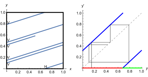
Figure 1. Left: Linear flow on the torus with initial condition $(0,0.15)$ and slope $W=1/\pi$. The symbol sequence of the shown orbit segment is $VVVHVV$. Right: Corresponding Poincaré map from $x=0$ to $x=1\equiv 0$ giving the exponents $n_{i}=0,0,1,0$.

2.1. Symbolic dynamics for integrable systems

Suppose now that our flow on $M$ is a Liouville integrable system with $2$ degrees of freedom. Then $M$ is a symplectic manifold $M$ of dimension $4$ endowed with $2$ smooth functions $G,H:M\to\mathbb{R}$ in involution, independent almost everywhere, one of which, $H$, we take to be the energy of the system. The pair $F=(G,H):M\to\mathbb{R}^{2}$ is called the integral map. The Liouville-Arnold theorem states that if $c$ is a regular value of the integral map, then every compact connected component of the pre image $F^{-1}(c)$ is a $2$-torus. Denote one of these tori by $\mathbb{T}_{c}$. Then in a neighbourhood $U$ of $\mathbb{T}_{c}$ one can introduce action-angle variables $(I_{1},I_{2},\theta_{1},\theta_{2})$, such that the dynamics is given by

$$\dot{\theta}_{j}=\omega_{j}(I_{1},I_{2}),\quad\dot{I}_{j}=0,\qquad j=1,2\,.$$

The tori are labelled by the value of the action $I=(I_{1},I_{2})$. On each torus the dynamics is straight line motion when viewed from the covering space $\mathbb{R}^{2}$ of that torus: $\theta_{i}(t)=\theta_{i}(0)+\omega_{i}(I)t$. When changing from one torus to another, $I$ and in general $\omega_{i}(I)$ will change, and hence the slope of the lines changes.

If the windows $S_{i}\subset M$ intersect the torus $\mathbb{T}_{c}$ transversally then they form a system of windows $\mathbb{T}_{c}\cap S_{i}$ (possibly empty) for the restricted linear dynamics on $\mathbb{T}_{c}$. In our situation of the planar two-center problem the windows will be horizontal or vertical lines: $\theta_{1}=const$ or $\theta_{2}=const$. With this in mind, the following example which goes back to Morse and Hedlund [14] is central to our work.

Example: Consider a linear flow on $\mathbb{T}^{2}=\mathbb{R}^{2}\mod\mathbb{Z}^{2}$ with positive slope $m=\omega_{2}/\omega_{1}$. As windows take the two two circles obtained by projecting the x-axis and the y-axis of $\mathbb{R}^{2}$ onto the torus. Denote their symbols ‘H’ for horizontal and ‘V’ for vertical. Lifted to the $xy$ plane, the windows yield the lines of graph paper intersecting at the lattice points. The lifted orbits are the lines

(1) $$y=mx+b.$$

Every such orbit has a unique symbol sequence as long as it stays away from lattice points.

The ratio of $H$’s to $V$’s in the symbol sequence of an orbit tends to the slope $m$ as the length of the orbit tends to infinity. The precise sequence of $H$’s and $V$’s depends on the initial condition $y_{0}$, i.e., on $b$. The resulting sequences are called “Sturnian sequences” after Morse and Hedlund coined this term in [14]. To describe this sequence let $\lfloor y\rfloor\in\mathbb{Z}$ denote the greatest integer less than or equal to $y$, for $y$ a real number. A bit of experimentation drawing lines on graph paper suggests that the associated symbol sequence always has the form

(2) $$\ldots VH^{n_{1}}VH^{n_{2}}VH^{n_{3}}\ldots$$

where each nonnegative integer $n_{i}$ is either $\lfloor m\rfloor$ or $\lfloor m\rfloor+1$. Which one though? To describe the $n_{i}$, let $\{y\}$ denote the fractional part of a real number $y$ so that $y=\lfloor y\rfloor+\{y\}$ with $0\leq\{y\}<1$. Use the Poincare map associated to cutting across the vertical circle: $y\mapsto y+m$ so as to obtain a sequence of points $y_{i}\mod 1$ on the circle, these being the orbit of $y_{0}$ uder the Poincare map, and their associated fractional parts. $\{y_{k}\}=\{y_{0}+km\}$. Then

(3) $$n_{k}=\begin{cases}\lfloor m\rfloor,&\text{if }\{y_{k-1}\}+\{m\}<1\\ \lfloor m\rfloor+1,&\text{if }\{y_{k-1}\}+\{m\}>1\\ \end{cases}\,.$$

Here we have started with the point at $(0,y_{0})$ and marked the initial ‘$V$’ in equation (2) as corresponding to “$s_{0}$” accordingly. An equivalent formula for the exponents is $n_{k}=\lfloor m+\{y_{k-1}\}\rfloor$.

Definition 1.

The sequence of integers $\{n_{k}\}_{k\in\mathbb{Z}}$ defined by equation (3), or the corresponding symbol sequence of $H$’s and $V$’s will be called the “Sturmian sequence for rotation number $m$ and intercept $y_{0}$”, assuming that the line $y=mx+y_{0}$ does not hit any lattice points.

Lemma 1.

Suppose that the slope $m$ is rational. Then when viewed as a periodic word, the Sturmian sequence associated to rotation number $m$ and intercept $y_{0}$ is independent of the choice of intercept. Thus we can speak of “the Sturmian word for $m$” in case $m$ is rational.

Proof. Suppose that $m=p/q$ is rational, with $p,q$ relatively prime. Then the initial conditions $(0,b)$, $0<b<1$ which pass thru the lattice points are those for which $b=i/q,i=1,2,\ldots,q-1$ and they cut the basic interval into $q$ equal intervals. Within any one of these intervals the sequence is constant, since the associated line $y=mx+b$ can be translated without hitting lattice points. What about when we move our initial condition $(0,b)$ to a different interval? Use the lattice translations to decompose all the vertical unit intervals between vertically adjacent lattice points into these $q$ equal segments. Because $p$ and $q$ are relatively prime, any line starting in the interval $0<y<1/q$ eventually hits all of the $q$ other segments. We can thus imagine starting at any one of these $q$ segments, but at a later time along the line, so arriving at a shifted version of the same sequence which corresponds to $b$ lying in this other segment. QED

Remark.

When $m$ is irrational the Sturmian word depends on the intercept $y_{0}$ in an interesting and nontrivial manner.

Remark.

Sturmian sequences arise in billiards [5], in the Henon map [6], and in twist maps of the cylinder [2].

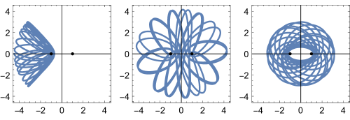
Figure 2. Orbits in the $(x,y)$-plane for the symmetric case $m_{1}=m_{2}=1/2$, $d=1$, and $h=-0.23$. Type Satellite (left) intersects the $x$-axis near one of the centers only. Type Lemniscate (middle) intersects the $x$-axis near both centers. Type Planetary (right) does not intersect the segment between the centers.

3. The Two Center Problem and its tori.

We consider a unit test particle moving in the $xy$ plane $\mathbb{R}^{2}$ attracted by two fixed masses of mass $m_{1}$ and $m_{2}$ called “centers” and located at the points $(-d,0)$ and $(d,0)$. The Hamiltonian in canonical coordinates $x,y,p_{x},p_{y}$ with symplectic form $dx\wedge dp_{x}+dy\wedge dp_{y}$ is

(4) $$H=\frac{1}{2}(p_{x}^{2}+p_{y}^{2})-\frac{m_{1}}{\sqrt{(x+d)^{2}+y^{2}}}-\frac{m_{2}}{\sqrt{(x-d)^{2}+y^{2}}}.$$

Euler [7] proved that the system is integrable with independent second integral

(5) $$G=\frac{1}{2}(xp_{y}-yp_{x})^{2}+\frac{1}{2}d^{2}p_{x}^{2}+dx\left(\frac{m_{1}}{\sqrt{(x+d)^{2}+y^{2}}}-\frac{m_{2}}{\sqrt{(x-d)^{2}+y^{2}}}\right)\,.$$

$(G,H)$ form our “integral map”, a map from phase space to the space of values of these two integrals.

Integration involves switching to regularizing variables for configuration space which are denoted $\lambda,\nu$ below. For details see section 7 below. These variables have the local effect of a Levi-Civita regularization about each of the two centers.

Definition 2.

By a regular torus $\mathbb{T}$ we mean a compact connected component of an inverse image of a regular value of the integral map, expressed in regularizing variables. By a regular periodic orbit we mean a periodic orbit without collisions lying on a regular torus.

Excluding the critical values of the integral map, there are precisely three topological types of tori, denoted by S, L and P. The projection of a torus of each type onto configuration space are as shown in figure 2. After regularization we can define “action-angle” variables with angles $\theta_{1}$, $\theta_{2}$. These angles identify a regular torus with $\mathbb{R}^{2}/\mathbb{Z}^{2}$. We will say a torus, expressed in these variables, has been “flattened”.

3.1. Windows, Syzygies

The phase space is $T^{*}(\mathbb{R}^{2}\setminus\Delta)$ where $\Delta=\{(-d,0),(d,0)\}$ are the collisions. When the test particle crosses the $x$-axis the three masses become collinear. The centers divide the $x$-axis into three intervals, labelled “1” for the right infinite interval $(-\infty,d)$, “2” for for the left infinite interval $(d,\infty)$. and “3” for the central finite interval $-d<x<d$. This labelling corresponds precisely to the syzygy sequence labelling of the references [12] and [10] mentioned above provided the test particle is labelled “3”, the right center as “1” and left center as “2”.

The inverse image of the collinear locus, with its three windows, drawn on the flattened torus is shown for each type in figure 3. These pictures are at the heart of our analysis. We continue to denote the inverse image of our syzygy windows 1, 2, and 3, under the regularization map, intersected with the torus, and flattened by the symbols 1, 2, or 3. These windows are a collection of orthogonal lines. How did a decomposition of a straight line – the $x$-axis – into intervals become a system of orthogonal lines? A regularization, qualitatively similar to the the Levi-Civita regularization, is needed to write down the action angle variables and hence express the torus. At the core of Levi-Civita regularization is the squaring map, the conformal map $\xi+i\eta\mapsto(x+iy)=(\xi+i\eta)^{2}$ under which the inverse image of a straight line through the origin becomes a “cross”: a pair of orthogonal lines, and this fact explains how the $x$-axis turned into a collection of orthogonal lines. See section 7 for details.

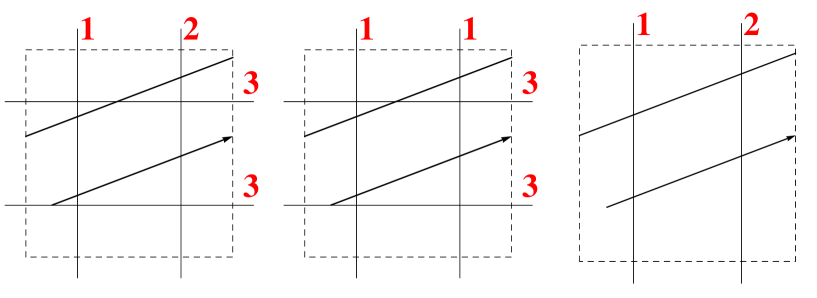
Figure 3. The torus (dashed) in angle variables $\theta_{1},\theta_{2}$ with a trajectory and windows with corresponding symbols for type L (Lemniscate), S, (Satellite), P (Planetary). The corresponding symbol sequences for the orbit segment shown (line with an arrow, continued with periodic boundary conditions) are 312132, 311131, 1212, respectively.

4. Main results: syzygy sequences for the two center problem

The main result is

Theorem 1.

The periodic syzygy sequences for regular periodic orbits of the two center problem are of the form: L type: $13^{n_{1}}23^{n_{2}}13^{n_{3}}2\ldots 3^{n_{s}}$ (1’s and 2’s alternating) S type: $13^{n_{1}}13^{n_{2}}13^{n_{3}}1\ldots 3^{n_{s}}\,\,\,$ or $\,\,\,23^{n_{1}}23^{n_{2}}23^{n_{3}}\ldots 23^{n_{s}}$ P type: $(12)^{q}$ where the exponents $n_{i}$ are those of the Sturmian sequence (3) associated to the rational rotation number $W$ for that orbit’s torus (Definition 1). The length of the fundamental sequence is $2(p+q)$ where $W=p/q>0$. (For the range of possible rotation numbers see the final sentence of the next theorem.)

See figure 4 for examples of periodic type L orbits, their rotation numbers and syzygy sequences for equal masses. See figure 5 for examples of periodic type S orbits, their rotation numbers and syzygy sequences in a case of distinct masses.

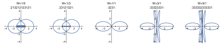
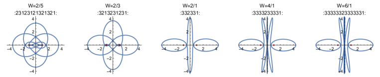
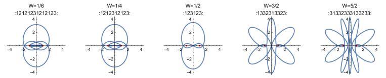
Figure 4. Periodic orbits of Lemniscate type in the $(x,y)$ plane for the equal mass case $m_{1}=m_{2}=1/2$, $d=1$, $h=-0.23$ with various rotation numbers $W$. To the right more oscillations along the $y$-axis are added, to the left more oscillations along the $x$-axis are added, keeping the parity of $W$ the same along each row.

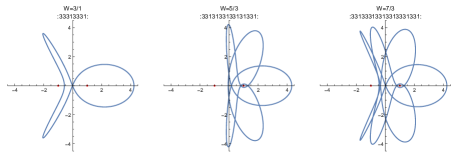
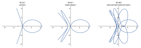
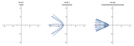
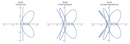
Figure 5. Periodic orbits of Satellite type in the $(x,y)$ plane for the asymmetric case $m_{1}=1/3$, $m_{2}=2/3$, $d=1$, $h=-0.23$ with various rotation numbers $W$. Parity if the same along each row. The third row shows tori of type S1, all other of type S2.

Missing periodic orbits. The only periodic orbits whose sequences are not represented in the theorem above are those on non-regular level sets of the integral map. There are five such families of periodic orbits corresponding to critical values of the integral map, see figure 11. Three of these five correspond to periodic orbits that are collinear, i.e. they move along the axis $y=0$ that contains the two centers, and as such don’t have well define syzygy sequences. The other two families have either syzygy sequence 3 (separating type L from type S, orbit is on the symmetry axis $x=0$ when then masses are equal), or syzygy sequence 12 repeated (orbit encircling both centers, the outer boundary of type P).

Our main result is a corollary of the next theorem which includes the infinite aperiodic orbits – the dense windings on the tori.

Theorem 2.

The syzygy sequences realized by regular non-collision orbits for the two-center problem are precisely one of the following possibilities:

$$\ldots 121212\ldots,\text{in the P case,}$$

$$\dots 13^{n_{1}}23^{n_{2}}13^{n_{3}}2\dots,\text{ in the L case,}$$

$$\dots 13^{n_{1}}13^{n_{2}}13^{n_{3}}1\dots,\text{ or }\dots 23^{n_{1}}23^{n_{2}}23^{n_{3}}2\dots\text{ in the S case}$$

In the last two cases the integer sequence $n_{i}$ occurring is the Sturmian sequence (Definition 1) associated to the rotation number $W=W(g,h)$ of that orbit’s torus $\mathbb{T}(g,h)$, and any possible intercepts $y_{0}$. The range of rotation numbers $W$ determining the $n_{i}$ can be read off from tables 10 and 11 below.

Remark.

The rotation number $W$ only depends on the regular values $g,h$ and not on the choice of torus when $F^{-1}(g,h)$ consists of more than one torus. This “coincidence” is a consequence of the fact that the two-center problem is integrable in elliptic functions, and moreover that the differentials that define the rotation numbers are of first kind.

The main theorem has some simple consequences.

Corollary 3.

In any orbit on a regular torus of type L or S the number of consecutive 3s is either $n$ or $n+1$ where $n$ is the integer part of $W$.

Proof.

This follows directly from the definition of the Sturmian sequence. ∎

Corollary 4.

In all cases symbol 1 and 2 never appear adjacent to each other (“no 1 or 2 stutters”). Lemniscate orbits with $W<1$ have no stutters, while for $W>1$ they have 3-stutters. Every Satellite orbit has at least one 3-stutter.

Proof.

For type L the symbols 1 and 2 alternate, so there cannot be stutters of these symbols. For type S there would be 1- or 2-stutters if any $n_{i}=0$, however we have numerically verified that $W>1$ for type S, so by equation (3) we have $n_{i}>0$. At least one 3-stutter, i.e. one $n_{i}=2$, must occur when $W>1$, because then the line in figure 3 with slope $>1$ must intersect the vertical lines of symbol 3 at least once. ∎

5. Guts of the proof.

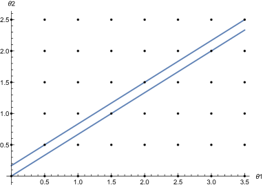
Figure 6. Two solution curves with $W=2/3$ bounding a region of orbits without collisions. Half-lattice points correspond to collisions.

Each regularized Liouville torus $\mathbb{T}=\mathbb{T}(g,h)$ maps to configuration space by composing its inclusion into regularized $\lambda,\nu,p_{\lambda},p_{\nu}$-phase space and projecting the regularized phase space onto the usual $xy$ configuration space. The windows on $\mathbb{T}$ are the inverse image of the collinear locus (the $x$-axis) with respect to this map. We will show in sections 7 and 8 that these windows are a finite collection of horizontal and vertical lines, positioned as indicated in figure 3 according to the cases S, L or P. Here “horizontal” or “vertical” mean that when we coordinatize $\mathbb{T}$ in standard angle variables $\theta_{1}\theta_{2}$ of “action-angle” as $\mathbb{R}^{2}/\mathbb{Z}^{2}$, then these lines are parallel to the $\theta_{1}$ or the $\theta_{2}$ axes. Lifted to the universal cover, then we get almost exactly the ‘graph paper picture’ used for writing Sturmian words. In the S and L cases we have 4 lines in all, a horizontal pair and a vertical pair, see figure 3. The parallel lines in each pair are separated by 1/2 a lattice unit. In the P case we have only the two vertical lines separated by 1/2 a unit. The intersections of the lines represent collisions of our test particle with the appropriate primary. This pattern is represented on the plane as a doubly periodic pattern of parallel lines.

On a fixed torus $\mathbb{T}=\mathbb{T}(g,h)$ the solution curves are a family of parallel straight lines $y=Wx+b$ with $W=W(\mathbb{T})$ constant, and $b$ varying. Here we have changed variables so $x=\theta_{1}$, $y=\theta_{2}$ so as to conform to the discusion of subsection 2.1. The torus supports periodic solutions if and only if $W$ is rational. A finite number of these solutions will have collisions. Those remaining have a syzygy sequence.

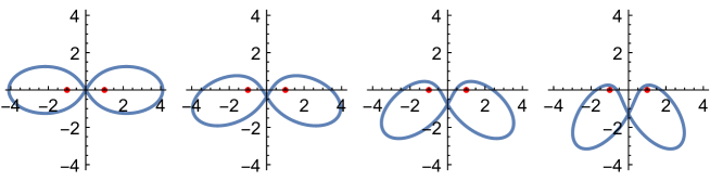
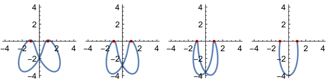
Figure 7. Orbits of type L with $W=1$ and syzygy sequence $1323$ for $h=-0.23$ and $m_{1}=m_{2}=1/2$ for a sequence of initial conditions with different $\nu_{0}=i\pi/14$, $i=0,\dots,7$ and the same $\lambda_{0}=0$ on the same torus. For $\nu_{0}=0$ the orbit has additional discrete symmetry, while for $\nu_{0}=\pi/2$ it is a collision-collision orbit.

The following is essentially a restatement of theorem 2:

Lemma 2.

On a fixed regular rational torus $\mathbb{T}=\mathbb{T}(g,h)$ all collision-free solutions have the same periodic syzygy sequence. This sequence is as described in theorem 2, where $W=W(g,h)$ is the rotation number of $\mathbb{T}$. If $W=p/q$ then the length of this common syzygy sequence is $2(p+q)$ in the S and L cases, and $2q$ in the $P$ case.

Proof.

Let $W=p/q$ be given, and the labelled set of vertical and (possibly) horizontal lines be given. Each solution is a straight line of slope $p/q$, see figure 6

P case. There are no horizontal lines, so no collisions. Vertical lines marked with 1 and 2 alternate. The only possible sequence is $(12)^{s}$ for some power $s$. Each straight line cuts across $q$ basic units in the horizontal direction before closing, so that we have $s=q$.

S and L cases. Fix attention on one of the 4 collision points: these being the intersection of the vertical and horizontal lines. Shift the fundamental domain describing the torus so that this point is at the origin. Collision solutions are those passing through a lattice point and we throw these out. Because the line pairs are half a unit a part, it makes sense to magnify the lattice. Consider the new lattice $((1/2)\mathbb{Z})^{2}$ in the plane, the torus’s universal cover, whose points represent collisions. We are now in a situation identical to that of subsection 2.1, except that the lines have different labellings! The independence of the sequence on the initial condition of the torus follows from lemma 1 of subsection 2.1. Keeping track of the labelling leads to the sequences described in theorem 2. Everything has already been done by Morse and Hedlund, as described in section 2.1, with the exception of the counting of sequence length. For this count, observe that there are 2 horizontal lines per vertical unit and 2 vertical lines per horizontal unit. Every solution must traverse $q$ horizontal units and $p$ vertical units and so crosses $2q+2p$ lines in all.

∎

Remark.

The fact that the symbol sequences are the same for solutions on a fixed rational torus does not mean that these solutions are the same! Indeed, they sweep out a torus-full of solutions. In figure 7 we show the deformation of the type L orbit with $W=1/1$ when the initial condition on the torus is changed. The orbit undergoes a deformation from a symmetric state all the way to a collision orbit. Note that for a generic non-integrable perturbation one expects that almost all of these periodic orbits will be destroyed.

6. Collision orbits

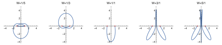
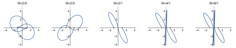
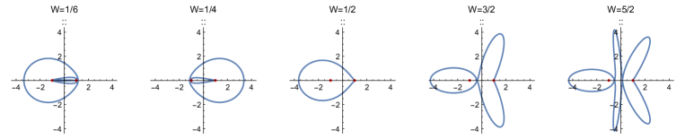
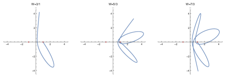
Figure 8. Collision orbits of Lemniscate type in the $(x,y)$ plane for the equal mass case $m_{1}=m_{2}=1/2$, $d=1$, $h=-0.23$ with various rotation numbers $W$. To the right more oscillations along the $y$-axis are added, to the left more oscillations along the $x$-axis are added, keeping the parity of $W$ the same along each row. Collision orbits with $W=odd/even$ visit the same collision twice. The last row shows some brake-collision orbits of Satellite type (same parameters).

In figure 8 we show some collision orbits, which are found on tori with rational $W$ for initial conditions with $\lambda=0$ and $\nu=\pm\pi/2$, as we now show.

Corollary 5.

Orbits that connect two collisions lie on a regular torus with rational rotation number $W$.

Proof.

Collision points are half integer lattice points in the covering plane of the torus. Any line connecting such lattice points has rational slope. ∎

Corollary 6.

Orbits that have a single collision lie on a regular torus with irrational rotation number $W$.

Proof.

A line with rational slope that hits a half integer lattice collision point in forward time, will also hit another such point in backward time. Hence only lines with irrational slope can hit one lattice point (in either forward or backward time). ∎

Corollary 7.

Regular orbits that keep a finite distance from collisions lie on a regular torus with rational rotation number $W$ (unless in the P family, which has no collisions).

Proof.

A line with irrational slope will come arbitrarily close to a half integer lattice point. Hence the only lines that keep a finite distance have rational slope, unless they are collision-collision orbits, as described in the previous corollary. ∎

Corollary 8.

Any regular torus of type S or type L with rational rotation number has exactly two collision-collision orbits.

Proof.

This follows from lemma 2, the fundamental region covered by two copies of the strip shown in figure 6 has exactly two collision-collision orbits, corresponding to the two lines shown in the figure. ∎

7. Euler’s Problem of Two Fixed Centers

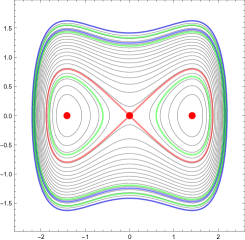
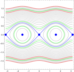
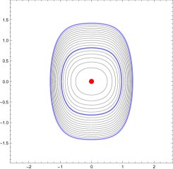
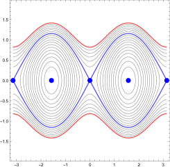
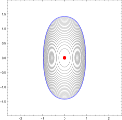
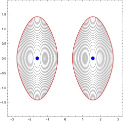
Figure 9. Level lines of $H_{\lambda}$ (left) and $H_{\nu}$ (right) with critical points marked by red and blue dots, respectively, and pre-images of critical values in the corresponding color. Green contours denote the levels corresponding to the three example shown in Fig. 1. Always $m_{1}=m_{2}=1/2$, $d=1$. Top: $h=-1/6>h_{\lambda}$, types S, L, and P occur. Middle: $h=-2/3>h^{*}$, types S, and L occur. Bottom: $h=-6/5<h^{*}$, type S only.

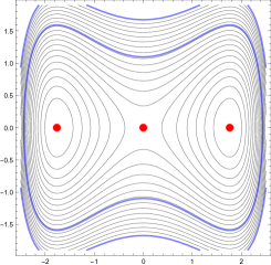
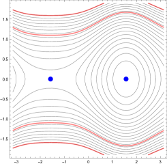
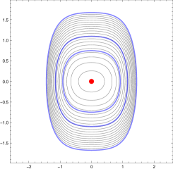
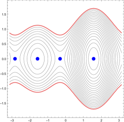
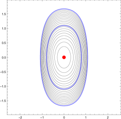
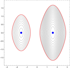
Figure 10. Level lines of $H_{\lambda}$ (left) and $H_{\nu}$ (right) with critical points marked by red and blue dots, respectively, and pre-images of critical values in the corresponding color. Always $m_{1}=3/10$, $m_{2}=7/10$, $d=1$. Top: $h=-1/6>h_{\nu}$, types S’, L, and P occur. Middle: $h=-2/3>h^{*}$, types $\mathrm{S^{\prime}}$, S, and L occur. Bottom: $h=-6/5<h^{*}$, type S and S’ only.

In this section we recall what we need from the detailed description of the solution to the problem of two fixed centers given by [17]. Many of the results here are refered to in theorem 2.

Without loss of generality we set $d=1$ so that the centres are place at $(1,0)$ and (-1,0). Standard confocal elliptic coordinates $(\lambda,\nu)$ are then defined by the relation $x+iy=\cosh(\lambda+i\nu)$. We will slightly alter the standard relation, defining instead

$$x+iy=\sin(\nu+i\lambda)\,.$$

In terms of real and imaginary parts we have

$$(x,y)=(\cosh\lambda\sin\nu,\sinh\lambda\cos\nu)$$

Combined with the time reparameterization $\tau=\tau(t;\lambda,\nu)$ given by $\mathrm{d}t=(\cosh^{2}(\lambda)-\cos^{2}(\nu))\mathrm{d}\tau$, these variables regularize and separate the Hamiltonian at energy $h$:

$$\tilde{H}=\tilde{H}(\lambda,\nu,p_{\lambda},p_{\nu};h):=(H-h)\frac{\mathrm{d}t}{\mathrm{d}\tau}=H_{\lambda}(\lambda,p_{\lambda})+H_{\nu}(\nu,p_{\nu})$$

into two one-degree of freedom Hamiltonians:

$$H_{\lambda}(p,q;h) =\frac{p^{2}}{2}-(m_{1}+m_{2})\cosh q-h\cosh^{2}q,$$

$$H_{\nu}(p,q;h) =\frac{p^{2}}{2}+(m_{1}-m_{2})\sin q+h\sin^{2}q\,.$$

We must take the value of $\tilde{H}$ to be $0$ since we want $H=h$. Then we have that $H_{\lambda}(p,q)=-g$ and $H_{\nu}(p,q)=g$ where $g$ is the value of the separation constant which is also the second integral $G$, see equation (5). (Our $H_{\lambda},H_{\nu}$ differ from those in [17] by $-h\cosh^{2}(\lambda),h\sin^{2}(\nu)$ respectively.)

The map $(\lambda,\nu)\to(x,y)$ defines a branched cover of the $(x,y)$ plane, branched over the two centres. The inverse image of the $x$ axis ($y=0$) consists of the lines $\lambda=0$ and $\nu=\pm\pi/2+2k\pi,k\in\mathbb{Z}$. The intersections of these lines, $(\lambda,\nu)=(0,\pm\pi/2+2k\pi)$ get mapped in an alternating way to the two centres. The inverse image of window 3 (the segment between the two centers) corresponds to the line $\lambda=0$. The inverse image of window 1 corresponds to the lines $\nu=-\pi/2+2k\pi$. The inverse image of window 2 corresponds to the lines $\nu=\pi/2+2k\pi$. It is central to our analysis that the symbols 1, 2 and 3 are defined by coordinate lines in the separating variables.

The energy has a single critical point lying on window 3 corresponding to an unstable equilibrium lying on the $x$-axis at the point where the forces exerted by the two centres balance. The associated critical value of energy is

(6) $$h_{*}=-(\sqrt{m_{1}}+\sqrt{m_{2}})^{2}/2$$

and serves as a bifurcation value. We view $\nu$ as an angular coordinate so that $(\lambda,\nu)\in\mathbb{R}\times S^{1},S^{1}=\mathbb{R}/2\pi\mathbb{Z}$. Then the Hill region for energy $h$ is the domain

$$\text{ Hill}(h)=\{(\lambda,\nu):\exists p_{\lambda},p_{\nu}\text{ such that }\tilde{H}(\lambda,\nu,p_{\lambda},p_{\nu};h)=0\}\subset\mathbb{R}\times S^{1}\,.$$

For $h<h^{*}$ the Hill region consists of two disjoint disks, one disc about each centre. These discs merge at the equilibrium for $h=h^{*}$. For $0>h>h_{*}$ the Hill region is a connected domain, topologically an annulus $S^{1}\times I$, wrapping once around the cylinder.

See Fig. 9 and  10 for phase portraits of the two one-degree of freedom Hamiltonians for various values of the masses. In these figures we make a number of contour plots in order to indicate how the one-degree-of-freedom systems combine to describe the two-degree-of-freedom system.

We now collect known facts about the critical values of the one-degree of freedom Hamiltonians and the implications these facts have for the critical values of the integral map $(G,H)$, see [17] for details.

Throughout we impose the condition $h<0$ since if $h\geq 0$ all motions are unbounded. We set

(7) $$h_{\lambda}=-(m_{1}+m_{2})/2\quad\text{ and }\quad h_{\nu}=-|m_{1}-m_{2}|/2,$$

and

(8) $$\kappa_{\pm\sigma}(h) =h+\sigma|m_{1}\pm m_{2}|,\quad\sigma=\pm$$

$$\chi_{\pm}(h) =-\frac{(m_{1}\pm m_{2})^{2}}{4h}\,.$$

Here the first subscript $+$ refers to critical values of $H_{\lambda}$, and the $-$ to critical values of $H_{\nu}$.

Critical values of $H_{\lambda}$. For $h<h_{\lambda}$ the function $H_{\lambda}(\cdot,\cdot,h)$ has exactly one critical value, $-\kappa_{++}$. For $h_{\lambda}<h$ the function has exactly two critical values $-\kappa_{++}$ and $-\chi_{+}$.

Critical values of $H_{\nu}$. For $h_{\nu}<h$ the function $H_{\nu}(\cdot,\cdot,h)$ has exactly two critical values $\kappa_{--}$ and $\kappa_{-+}$. For $h<h_{\nu}$ the function has three critical values $\kappa_{--}$, $\kappa_{-+}$, and $\chi_{-}$.

Critical and Regular values of the integral map. We can deduce the critical and regular values of the integral map $(G,H):T^{*}(\mathbb{R}\times S^{1})\to\mathbb{R}^{2}$ immediately from the above description of the critical values of the one-degree of freedom Hamiltionians and the separation of variables. The critical values of the map consists of the union of either four or five analytic curves depending on the values of the masses. See figure  11. Two or three of these curves are straight lines with slope 1. The remaining two curves are arcs of hyperbolas. The lines are $g=\kappa_{++}(h)$ , $g=\kappa_{-+}(h)$, and $g=\kappa_{--}(h)$. The arcs of hyperbolas are given by $g=\chi_{+}(h)$ for $h_{\lambda}\leq h$ and $g=\chi_{-}(h)$ for $h^{*}\leq h<h_{\nu}$. The image of the integral map is the region bounded between the leftmost and rightmost of these curves (remember: $h<0$ always!). This image is divided by the curves into three or four simply connected curvilinear domains whose interiors consist of the map’s regular values. These regions, henceforth called the “regular regions” are denoted by the symbols S’, S, L, P as indicated in the figures. The preimage of a point in region S or P is two disjoint 2-dimensional tori, while if the point is in S’ or L this preimage is a single torus. The terminology goes back to Charlier [4] and Pauli [15]. S and S’ stands for satellite, L for Lemniscate, and P for planetary.

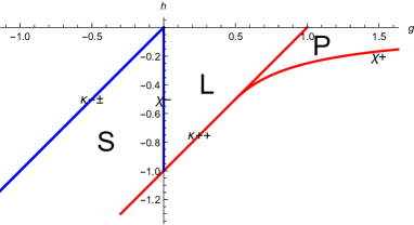
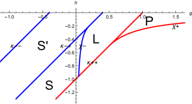
Figure 11. Critical values of the energy momentum map $(G,H)$ in the symmetric case $m_{1}=m_{2}=1/2$ (left) and in the asymmetric case $m_{1}=3/10$, $m_{2}=7/10$ (right). The regions of regular values are marked by S, L, P, for satellite, lemniscate, and planetary type, respectively. Blue lines are critical values of $H_{\nu}$; red lines are critical values of $H_{\lambda}$.

Our one-degree of freedom systems have period functions $T_{\lambda}(g,h)$ and $T_{\nu}(g,h)$ defined by an integral over the curve $H_{\lambda}(\cdot,\cdot,h)=-g$ and $H_{\nu}(\cdot,\cdot,h)=+g$. These period functions are analytic within each regular region of the $(g,h)$ plane. Our tori $\mathbb{T}(g,h)$ admit a natural homology basis, or coordinate system, corresponding to our separation of variables. We always define the rotation number $W$ in terms of this basis. Then our rotation number is

(9) $$W(g,h)=T_{\nu}(g,h)/T_{\lambda}(g,h)$$

which is a piecewise analytic function. We give explict formulae for $W$ further on. One surprise is that $W$ only depends on the value $(g,h)$ of the integral map in the case S where there are two tori for a given $g,h$: the value of the rotation number on these two tori is the same. Another surprise is that $W$ is analytic across the curve separating the region S from S’.

See Fig. 12 (bottom) for a plot of $W$ for energy $h=-1/4$ in the symmetric case. For this energy all three types S, L, and P occur.

The function $T_{\lambda}$ has discontinuity only along the red singular curves of figure 11 so has two ‘branches’ denoted $T_{\lambda 3}$ and $T_{\lambda 0}$ the first having domain formed by the union of S, S’ and L, while the second branch has domain P. (In case S’ is empty the first domain is just S union L.) The function $T_{\nu}$ has its only discontinuity along the blue singular curves of figure 11 so also has two branches, denoted $T_{\nu o}$ and $T_{\nu r}$, the first branch having domain the union of S and S’ and the second branch $T_{\nu r}$ having domain the union of P and L. See figure 13.

Consequently, the three branches of $W_{S,L,P}$ of the rotation number are given by:

$$W_{S}(g,h)=\frac{T_{\nu o}(g,h)}{T_{\lambda 3}(g,h)},\quad W_{L}(g,h)=\frac{T_{\nu r}(g,h)}{T_{\lambda 3}(g,h)},\quad W_{P}(g,h)=\frac{T_{\nu r}(g,h)}{T_{\lambda 0}(g,h)}\,,$$

For us, the crucial property of the rotation number $W$ is its range. If we fix $h$, and let $g$ vary, the rotation numbers sweep out an interval $[W_{min}(h),W_{max}(h)]$ which have the following dependence on energy $h$.
For type L:

(10) $$\begin{array}[]{c|cc}h&W_{min}&W_{max}\\ \hline\cr 0>h>h_{\lambda}&0&\infty\\ h_{\lambda}>h>h^{*}&W_{L}(\kappa_{++},h)&\infty\\ \end{array}$$

For type S:

(11) $$\begin{array}[]{c|cc}h&W_{min}&W_{max}\\ \hline\cr 0>h>h^{*}&W_{S}(\kappa_{--}(h),h)&\infty\\ h^{*}>h&W_{S}(\kappa_{--}(h),h)&W_{S}(\kappa_{++}(h),h)\end{array}$$

where the critical values $\kappa_{++}(h),\kappa_{-+}(h),\kappa_{--}(h)$ and $h_{\nu}$, $h_{\lambda}$ were defined in equations (8) and (7) above.

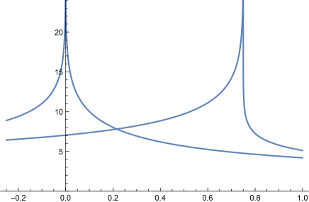
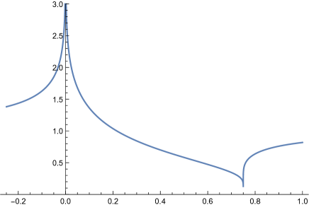
Figure 12. The period $T_{\nu}$ (diverging at 0) and $T_{\lambda}$ (diverging for positive $g$) (both top) and the rotation number $W=T_{\nu}/T_{\lambda}$ (bottom) all for $h=-1/4$, $m_{1}=m_{2}=1/2$, $d=1$. The type of corresponding tori is S, L, P from left to right, separated by singularities.

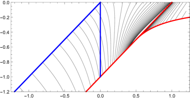
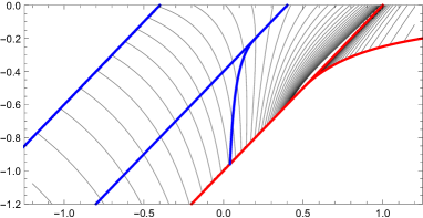
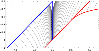
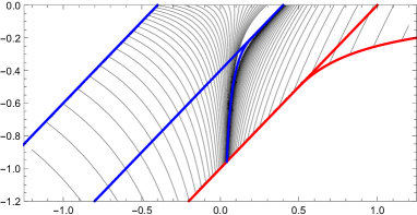
Figure 13. Contours of constant period $T_{\lambda}$ (top) and $T_{\nu}$ (bottom) for the symmetric case $m_{1}=m_{2}=1/2$ (left) and an asymmetric case $m_{1}=3/10$, $m_{2}=7/10$ (right).

We now proceed to determine the functional forms of the period functions, and hence of the rotation number. We have summarized their forms in Fig. 13. We use the standard method of period computation from the classical mechanics of one-degree of freedom systems (e.g. [9]). Let $\Psi(q,p)$ denote either $H_{\nu}(q,p;h)$ or $H_{\lambda}(q,p;h)$. $\Psi$ has the form $\frac{1}{2}p^{2}+V(q,h)$. The first of Hamilton’s two equations reads $dq/d\tau=p$ so that $d\tau=\frac{dq}{p}$. Solutions must lie on energy curves $\{\Psi=c\}$, $c=\pm g$, which consist for us of one or two topological circles. Choose a component $C$ for a given constant $c$. The time $T$ to traverse $C$ is the corresponding period $T$ which we want to compute. This time is given by the integral

$$T=\int_{C}d\tau=\int_{C}\frac{dq}{p}.$$

(One can solve for $p$ in terms of $q$ : $p=\pm\sqrt{2(c-V(q;h)}$ and use the time-reversal symmetry to rewrite this as $T=2\int_{q_{min}}^{q_{max}}\frac{dq}{\sqrt{2(c-V(q;h)}}$.) In our cases the variable $q$ is either $\nu$ or $\lambda$ and the variable $p$ is either $p_{\nu}$ or $p_{\lambda}$ The substitution $z=\sin\nu$ or $z=\cosh\lambda$ converts the integrand $\frac{dq}{p}$ to the integrand $\frac{dz}{P}$ where the integral in the new variables is around the loop corresponding to our choice $C$ which lies on the Riemann surface:

$$P^{2}=\begin{cases}2(1-z^{2})(+g+(m_{1}-m_{2})z+hz^{2}),\qquad\nu\text{ case}\\ 2(1-z^{2})(-g+(m_{1}+m_{2})z+hz^{2}),\qquad\lambda\text{ case }\\ \end{cases}$$

The integral $\int\frac{dz}{P}$ over the closed loop is a complete elliptic integral which can be expressed in terms of Legendre’s complete elliptic integral $\operatorname{K}(k^{2})$ with modulus $k$.

For the symmetric case $m_{1}=m_{2}$ we find

$$T_{\nu o}(g)=\frac{4}{\sqrt{-2h}}\operatorname{K}(k^{2}),\text{ for }g<0,\quad$$

$$T_{\nu r}(g)=\frac{4}{k\sqrt{-2h}}\operatorname{K}(1/k^{2}),\text{ for}g>0,$$

$$\text{ where }\quad k^{2}=1-\frac{g}{h},$$

Expressions of elliptic integrals in terms of Legendre’s standard integrals can, e.g., be found in [3]. Legendre’s $\operatorname{K}$ is a smooth monotonically increasing function that maps $k^{2}\in(-\infty,1)$ to $(0,\infty)$.

To write down the period $T_{\lambda}$ and to treat the asymmetric case $m_{1}\neq m_{2}$ introduce

$$k_{\pm}^{2}=\frac{1}{2}+\frac{g+h}{2\sqrt{4gh+(m_{1}\pm m_{2})^{2}}},\quad f_{\pm\sigma}=\frac{\sqrt{2}}{\sqrt{\sigma(-1-\frac{g}{h})-\frac{\sqrt{4gh+(m_{1}\pm m_{2})^{2}}}{h}}}$$

where $\sigma=0$ or $\sigma=1$. Then the $\lambda$-periods are

$$T_{\lambda 3}(g,h)=\frac{4}{\sqrt{2|h|}}f_{+0}\operatorname{K}(k_{+}^{2}),\text{ for }g<\kappa_{++}(h)$$

$$T_{\lambda 0}(g,h)=\frac{2}{\sqrt{|h|}}f_{+1}\operatorname{K}(1/k_{+}^{2}),\text{ for }\kappa_{++}(h)<g<\chi_{+}(h)$$

When $h>h_{\lambda}$ the modulus $k_{+}^{2}$ is monotone in both cases, increasing and decreasing, respectively. Now $f_{+0}(g)$ is always monotonically increasing, so that $T_{\lambda 3}$ is monotonically increasing in this energy range.

Note that since without loss of generality we can set $m_{1}+m_{2}=1$, the $T_{\lambda}$ periods do not change with parameters, only their domain of definition in the integral image changes. In particular the periods $T_{\lambda}$ in the symmetric case $m_{1}=m_{2}$ and the asymmetric case $m_{1}\not=m_{2}$ are given by the same functions.

For oscillations of $\nu$ (when $m_{1}\not=m_{2}$) the period is

$$T_{\nu o}(g,h)=\frac{4}{\sqrt{2|h|}}f_{-0}\operatorname{K}(k_{-}^{2})$$

where for $h>h_{\nu}$ the domain is $g<\kappa_{-+}(h)$ and the modulus is monotone, while for $h<h_{\nu}$ the domain is $g<\chi_{-}$ and $k_{-}^{2}$ passes through zero at $h\pm(m_{1}-m_{2})$. The formula is valid in region S and in region S’, in region S it gives the period for both tori of type S, around either center.

For rotations of $\nu$ (when $m_{1}\not=m_{2}$) there are two cases depending on whether the elliptic curve has 2 real or 4 real branch points. A formula that is valid in both cases is defined via

$$k_{c}^{2}=\frac{1}{2}-\frac{g+h}{2\sqrt{(g-h)^{2}-(m_{1}-m_{2})^{2}}}$$

and

$$T_{\nu r}(g,h)=\frac{4}{\sqrt{2}((g-h)^{2}-(m_{1}-m_{2})^{2})^{1/4}}K(k_{c}^{2})\,.$$

When there are four real branch points the sign of $k_{c}^{2}$ is negative, otherwise $k_{c}^{2}$ is positive. Moreover, when $h<h_{\nu}$ the modulus $k_{c}^{2}$ is monotonically decreasing. When $h>h_{\nu}$ the modulus is monotonically increasing from $-\infty$ to 0, which occurs at the boundary of the Lemniscate region for $g=\kappa_{++}$.

The functions $T_{\nu o}(g,h)$ and $T_{\nu r}(g,h)$ are monotone functions of $g$, for $h$ fixed, because $K(k^{2})$ is monotonically increasing, and $k^{2}(g)$ is linear in $g$ and increasing for $h<0$. So $T_{\nu o}(g)$ is monotonically increasing and diverges for $g\to 0_{-}$. Now $1/k^{2}(g)$ is monotonically decreasing for $g>0$ and so as a function of $g$, $T_{\nu r}$ is the product of two monotonically decreasing functions, and hence monotonically decreasing. It diverges for $g\to 0_{+}$.

Conjecture. The period function $T_{**}(g,h)$ and rotation function $W_{*}(g,h)$ are monotone functions of $g$ within their domains of analyticity.

Numerical experiments support this conjecture.

Note that in the S-region the modulus $k_{-}^{2}$ is negative, and approaches $-\infty$ at the boundary to L. Similarly, in the upper parts of the L- and P-region the modulus $k_{c}^{2}$ becomes negative, and on the boundary between L and S’ it approaches $-\infty$.

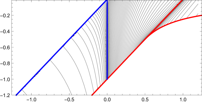
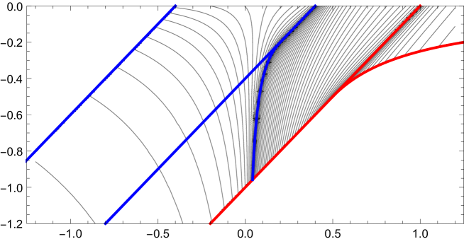
Figure 14. Contours of constant rotation number $W$ for the symmetric case $m_{1}=m_{2}=1/2$ (top) and an asymmetric case $m_{1}=3/10$, $m_{2}=7/10$ (bottom). The spacing of contours is even in $W$ or $1/W$, whichever is smaller.

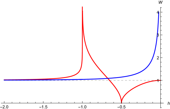
Figure 15. The boundary values of the rotation number $W$ along the leftmost curve of critical values (blue, see Fig. 11) which gives the minimum in S, and along the rightmost curve of critical values (red, see Fig. 11). The three smooth parts of the red curve correspond to the rightmost boundary values of tori of type S, L, and P, in that order. The red curves give the maximum in S, minimum in L, and maximum in P, respectively. Parameters are $m_{1}=m_{2}=1/2$, $d=1$.

The form of the period functions yield the following facts about the rotation number $W$. For $h_{\lambda}<h<h_{\nu}$ the rotation number $W_{L}(g)$ is a monotonically decreasing function. At the left boundary of the L region $W_{L}$ diverges to $+\infty$, while at the right boundary of the L region for $h>h_{\lambda}$ the rotation number $W_{L}$ approaches 0. For $m_{1}=m_{2}$ the limiting values of $W$ at the other families of critical values are as follows, see figure 15 for graphs of these functions.

To obtain tables 10 and 11 we need the minimum and maximum of $W(\cdot,h)$ within its various intervals of analyticity. For simplicity, in the following formulas we have set $m_{1}=m_{2}=1/2$). We compute that

• the minimum of $W_{S}(\cdot,h)$ is :

  $$W_{S}(\kappa_{--}(h),h)=\frac{\pi\sqrt[4]{4h^{2}+1}}{2\sqrt{-2h}\,\operatorname{K}\left(\frac{1}{2}+\frac{h}{\sqrt{4h^{2}+1}}\right)}$$

• the maximum of $W_{S}(\cdot,h)$ is, if finite, for $h<h^{*}$:

  $$W_{S}(\kappa_{++}(h),h)=\frac{1}{\pi}\sqrt{\frac{4h+2}{h}}\,\operatorname{K}\left(-\frac{1}{h}\right)$$

• the minimum of $W_{L}(\cdot,h)$ for $h^{*}<h<h_{\lambda}$ occurs at

  $$W_{L}(\kappa_{++}(h),h)=\frac{1}{\pi}\sqrt{-4h-2}\,\operatorname{K}(-h)$$

• the maximum of $W_{P}(\cdot,h)$ for $h_{\lambda}<h<0$ is:

  $$W_{P}(\chi_{+}(h),h)=\frac{2}{\pi}\sqrt{\frac{1-4h^{2}}{1+4h^{2}}}\,\operatorname{K}\left(\frac{1}{1+\frac{1}{4h^{2}}}\right)$$

In arriving at these facts we used that for the Lemniscate case $T_{\nu r}(g,h)$ is increasing with $g$ and that $T_{\lambda 3}(g,h)$ is decreasing with $g$, so that $W_{L}(g,h)$ is decreasing with $g$. We also used that the period $T_{\nu}$ diverges at the left boundary of the L-region, while the period $T_{\lambda}$ diverges at the right boundary of the L-region when $h>h_{\lambda}$, hence we arrive at the limiting behaviour of $W_{L}$. For a periodic orbit of type L or S with rational $W=p/q$ with co-prime $p$ and $q$ the period of the periodic orbit in original coordinates is $(pT_{\lambda}+qT_{\nu})/2$ where the factor $1/2$ accounts for the double cover.

8. Finishing up the proof of theorem 2.

We have established the range of the rotation numbers in the previous section. We established almost all of the proof in section 5. All that remains to prove is that the windows are situated as in figure 3. In particular, we have not yet shown that the line pairs are spaced $1/2$ a unit apart.

We saw that the two-center system separates into two one degree of freedom systems, that the separate torus coordinates correspond to these separate systems, with $\lambda,p_{\lambda}$ corresponding to the the $\theta_{2}$ motion and $\nu,p_{\nu}$ to $\theta_{1}$-motion. The windows on a given torus are vertical or horizonatl lines in the angle coordinaes since the collinear line $x=0$ corresponds to $\lambda=0$ or $\nu=const$ and since the axes of the torus correspond to one or the other of the separating coordinates: $\theta_{1}=\theta_{1}(\nu,p_{\nu};g,h)$, $\theta_{2}=\theta_{2}(\lambda,p_{\lambda};g,h)$. It follows that windows have the form $\theta_{1}=const$ or $\theta_{2}=const$. What constants? In other words, upon being projected onto either one-degree of freedom system, the windows correspond to points (or the empty set). But which points and how are they separated?

The explicit maps $\theta_{1},\theta_{2}$ as functions of mapping from the regularised coordinates $(\nu,\lambda,p_{\nu},p_{\lambda})$ are complicated expressions in terms of elliptic functions. Fortunately, this detailed information is not needed to answer our question due to the presence discrete symmetries for the separated Hamiltonians.

The symplectic involution $R_{\lambda}(\lambda,p_{\lambda})=(-\lambda,-p_{\lambda})$ leaves $H_{\lambda}$ invariant and hence commutes with the time evolution for that flow. The symplectic involution $R_{\nu}(\nu,p_{\nu})=(\pi-\nu,-p_{\nu})$ leaves $H_{\nu}$ invariant and so commutes with its time evolution (If $\tilde{R}_{\lambda},\tilde{R}_{\nu}$ denotes the extension of these involutions to the full regularized plane: for example, $\tilde{R}_{\nu}(\lambda,\nu,p_{\lambda},p_{\nu})=(\lambda,\pi-\nu,p_{\lambda},-p_{\nu})$ then the composition of the two involutions $\tilde{R}=\tilde{R}_{\nu}\circ\tilde{R}_{\lambda}$ is an involution on the double cover that leaves the original point $(x,y,p_{x},p_{y})$ fixed.) Rewritten in terms of angle coordinate, $\theta=\theta_{1}$ or $\theta_{2}$, either $R$ must commute with translation (since it commutes with its Hamiltonian flow) and thus is of the form $R(\theta)=\theta+p$ for some constant $p$. But since each $R$ is a nontrivial involution we must have that $p=1/2$.

For the $\lambda$ motion these window points are

• the two points $(0,p_{\lambda})$, $(0,-p_{\lambda})$ for the symbol 3. exchanged under $R_{\lambda}$. (Note that $p_{\lambda}=0$ above corresponds to the purely linear motion, and a degenerate torus, which we have exculded from considerations.)

• No symbol occurs.

As we just saw, $R_{\lambda}$ has the form $R_{\lambda}(\theta_{2})=\theta_{2}+1/2$, proving that the corresponding window points a half a unit apart, and so the corresponding lines are half a unit apart. In other words, the window for the symbol ‘3’ consists of two horizontal lines separated by half a lattice unit.

For the $\nu$ motion the window points are

• two points of the form $(\pi/2,\pm p_{\nu})$ for the symbol 1, exchanged by $R_{\nu}$.

• two points of the form $(-\pi/2,\pm p_{\nu})$ for the symbol 2, exchanged by $R_{\nu}$.

• a point $(\pi/2,p_{\nu})$ for symbol 1 and a point $(-\pi/2,\tilde{p}_{\nu})$ for symbol 2, where $p_{\nu}>0$ and $\tilde{p}_{\nu}>0$. There are two more such points with negative momenta which belong to a disjoint orbit of $H_{\nu}$ (“prograde” or “retrograde” motion) The two groups of points are mapped into each other by $R_{\nu}$.

By an argument identical to the $\lambda$-case, the two window points in each case are separated by a half, and so the corresponding vertical lines on the torus are separated by half a unit.

The resulting windows on the flattened torus for the three case L, S, P are thus as shown in figure 3.

The location of the windows relative to the origin of the flattened torus depends on the choice of origin of the two angles $\theta_{1}$ and $\theta_{2}$ and is irrelevant. The intersection of windows correspond to collisions, each of which appears twice since the regularisation led to a double cover of configuration space.

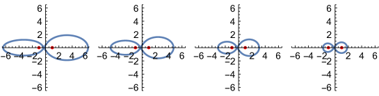
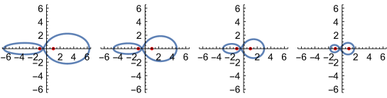
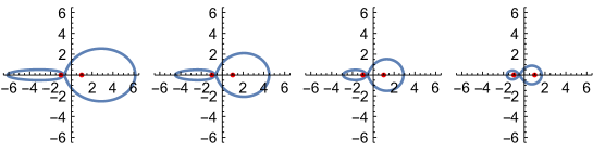
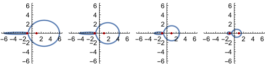
Figure 16. Orbit of type L with $W=1$ and syzygy sequence $1323$ for various values of $h=-0.15,-0.2,-0.3,-0.5$ from left to right and values of $m_{1}/m_{2}=0.5,0.4,0.3,0.2,0.1$ from top to bottom all with $m_{1}+m_{2}=d=1$. For type $L$ and $h>h_{\lambda}=-1/2$ all orbits exist in such 2-parameter families.

9. Additional Remarks

Remark: When $W=p/q$ with $q$ even the symbol sequence of type L repeats after $p+q$ symbols. When $q$ is odd the 2nd half of the symbol sequence is like the first with symbols 1 and 2 exchanged. For periodic orbits of type S the two halves of the symbol sequence are always identical.

Remark: There are no break-orbits of type L, since for these $p_{\nu}$ is always non-zero. For type S there are break-break orbits for $W=p/q$ with $p$ or $q$ even. When both $p$ and $q$ are odd the corresponding symmetric periodic orbit has reflection symmetry about the $x$-axis (but no break points), and the corresponding collision orbit is a break-collision orbit.

Remark: Discrete symmetry of periodic orbits. Let $W=p/q$.
Type L, arbitrary masses: If $q$ is odd, there is an orbit that has a crossing of the $x$-axis with a right angle. If $p$ is odd, there is an orbit that crosses the origin. In addition, if the masses are equal and $p$ or $q$ are even, there is an orbit that has a crossing of the $y$-axis with a right angle.

Type S, arbitrary masses: If $p$ or $q$ are even, there is a break-orbit. If $q$ is odd there is an orbit that has a crossing of the $x$-axis with a right angle.

Remark: A non-obvious consequence of the proof and the description from section 7 is that there are no bifurcations in the orbit structure and the symbol sequences of the L-region when changing the mass ratios or the energy within the range $(h_{\lambda},0)$. In particular all periodic orbits persists without bifurcations in this 2-parameter family. This strong resilience of orbits for sufficiently large energy is quite astonishing. It is illustrated for the $W=1/1$ orbit shown for various energies and various masses in figure 16. For smaller energies this is not true and orbits bifurcate away on the right boundary of region L.

Remark: Decreasing $h$ from $h_{\lambda}$ to $h^{*}$ (of the saddle equilibrium point) removes more and more rotation numbers by increasing the minimum value of the range $W\in(W_{L}^{min},\infty)$, thus only allowing orbits with more and more consecutive symbols 3, which describe close approaches to the isolated hyperbolic periodic orbit above the saddle. It is interesting to note that for any $h>h^{*}$ (even arbitrarily close), the whole complexity of orbits generated by $\{W\}$ passing through $[0,1)$ is still present, in fact there are always infinitely many such intervals.

Remark: For tori of type P the standard syzygy sequences do not separate tori, because symbol 3 does not occur and symbols 1 and 2 simply alternate for all allowed rotation numbers $W$. Instead of insisting on the usual symbols of the 3-body problem we can turn the construction around and choose a window on the torus so that we get similar symbol sequences with a different physical interpretation. As we already pointed out for separable integrable system the windows are best chosen as coordinate lines of the separating coordinate system. We choose an ellipsoidal coordinate line $\lambda=\lambda^{*}(h)=const$ such that all type P tori for the given energy intersect this line. When approaching the left boundary of the P-region the torus shrinks to an ellipse with $\cosh\lambda^{*}(h)=-(m_{1}+m_{2})/(2h)=h_{\lambda}/h>1$. Considering the phase portrait of $H_{\lambda}$ it is clear that all type P tori intersect the corresponding window. However, the intersection points are not spaced half-way around the torus, and hence would give a more complicated description. An alternative is to use $p_{\lambda}=0$ which does cut the torus twice with equal spacing. The physical meaning of this is to assign a symbol to the tangency with the caustic.

10. Conclusion

We have described all syzygy sequences which are realized in the two centre problem. They are encoded by Sturmian words as per theorem 1 and 2.

11. Some Open Problems.

Orbit Counts. This work began as a warm-up for understanding the syzygy sequences arising in the full planar three-body problems. Does it shed light on that problem, or on restricted versions of it? We take a peek at this question from the perspective of orbit counting.

Let $N(L)$ be the number of periodic orbits of length less than $L$ in a dynamical system. For chaotic systems such as Axiom A systems $N(L)$ grows exponentially with $L$, while for integrable systems one expects $N(L)$ to grow polynomially. Various theorems have been established relating $N(L)$ to the topological entropy of a system. In planar three-body problems we will instead let $N(L)$ be the number of distinct syzygy sequences of length $L$ which are suffered by some periodic orbit during one period. (The original $N(L)$, the number of orbits themselves is uncountably infinite since the orbits of a particular topological type, forms a continuum in an integrable system, sweeping out all of a torus, or a torus minus collisions. So we do not want to count individual orbits.) Being integrable, we expect that $N(L)$ grows polynomially for the two centre problem. Indeed, $N(L)$ grows like $L^{2}$. To estimate this growth, recall that altogether P orbits yield a single syzygy sequence $1212\ldots$. To count the number of sequences due to L and S orbits, recall that these sequences are encoded by their rational rotation number $W=p/q$, $W>0$ with the length $L$ of the sequence being $2(p+q)$. So $N(L)$ is bounded by the number of lattice points $(p,q)$ inside the diamond $|x|+|y|\leq\frac{1/2}{L}$, which is $\frac{1}{8}L^{2}$. We count both the S and L type, yielding the bound $N(L)\leq\frac{1}{4}L^{2}+1$.

On the other hand, if we use the strong force potential $-m_{1}/r_{1}^{2}-m_{2}/r_{2}^{2}$, then one can prove using variationally methods, that all syzygy sequences are realized in the two centre problem except for those with “stutters”, meaning two of the same type of symbols adjacent to each other. One estimates $N(L)\geq 3*2^{L-2}$ for the number of such symbols.

The two-centre problem fits within various one-parameter families of 2-degree of freedom Hamiltonian systems $H_{\lambda}(x,y,p_{x},p_{y})$. For example, by “spinning” the primaries we can fit it into a one-parameter family, parameterized by the spin rate of the primaries, which at the other endpoint becomes the restricted three-body problem. Or, by changing the potential, we can fit the problem into a one-parameter family which includes strong-force two center problem. How does $N_{\lambda}(L)$ depend on $\lambda$ for these other problems?

Sturn and twist As remarked above, Sturmian words arise generically in twist maps [2]. This “Sturmian thread” connecting the two centre problem to general twist maps gives us hope that enough twist-map structure persists as we turn on the spin parameter so that many of the periodic orbits or quasi-periodic irrational Sturmian type orbits will persist all the way to the restricted three body problem.

12. Acknowledgment

We thank Rick Moeckel (U. Minnesota, US) and Ivan Sterling (St Mary’s College, Maryland, US) for accompanying us on the initial leg of this journey. We thank Michael Magee (Princeton) for alerting us to the long history of “Sturmian words” going back to Morse and Hedlund. RM thanks the support of the NSF DMS1305844 grant and HD the Australian ARC DP110102001 grant. HRD would like to thank the UC Santa Cruz Department of Mathematics for their hospitality.

References

- [1] D. V. Anosov. Geodesic flows on closed Riemannian manifolds of negative curvature. Proc. Stekhlov Institute of Math., 90, 1967.
- [2] S. Aubry and P.Y Le Daeron. The discrete Frenkel-Kontorova model and its extensions. Physica, 8D:381–422, 1983.
- [3] P. F. Byrd and M. D. Friedman. Handbook of Elliptic Integrals for Engineers and Physicists. Springer, Berlin, 1971.
- [4] C. L. Charlier. Die Mechanik des Himmels. Veit & Comp., Leipzig, 1902.
- [5] H. R. Dullin and A. Bäcker. About ergodicity in the family of Limaçon billiards. Nonlinearity, 14:1673–1687, 2001.
- [6] H. R. Dullin, J. D. Meiss, and D. G. Sterling. Symbolic codes for rotational orbits. SIAM J. Appl. Dyn. Syst., 4(3):515–562, 2005.
- [7] Leonhard Euler. De motu corporis ad duo centra virium fixa attracti. In Opera Omnia: Series 2, volume 6, pages 209 – 246, 247 – 273. 1760.
- [8] J. Hadamard. Les surfaces á courbure opposées et leur lignes géodésiques. J. de Math. pures et appl., 4:27–73, 1898.
- [9] L.D. Landau and E.M. Lifshitz Classical Mechanics (Course of Theoretical Physics, volume 1 translated by J.B. Sykes and J.S. Bell Pergamom Press, 3rd edition, Oxford, 1976.
- [10] Richard Moeckel and Richard Montgomery. Realizing all reduced syzygy sequences in the planar three-body problem. Nonlinearity, 28(6):1919, 2015.
- [11] Richard Montgomery. Action spectrum and collisions in the planar three-body problem. Contemporary Mathematics, 292:173–184, 2002.
- [12] Richard Montgomery. Infinitely many syzygies. Archive for rational mechanics and analysis, 164(4):311–340, 2002.
- [13] M. Morse and G.A. Hedlund. Symbolic dynamics. Am. J. of Math., 60:815–866, 1938.
- [14] M. Morse and G.A. Hedlund. Symbolic dynamics II: Sturmian trajectories. Am. J. of Math., 62:1–42, 1940.
- [15] W. Pauli. Über das Modell des Wasserstoffmolekülions. Ann. Phys. (Leipzig), 68:177–240, 1922.
- [16] S. Smale. Diffeomorphisms with many periodic points. In S. S. Cairns, editor, Differential and Combinatorial Topology, pages 63–80. Princeton Univ. Press, 1963.
- [17] H. Waalkens, H. R. Dullin, and P. H. Richter. The problem of two fixed centers: bifurcations, actions, monodromy. Physica D, 196:265–310, 2004.
- [18] E. T. Whittaker. A Treatise on the Analytical Dynamics of Particles and Rigid Bodies. Cambridge University Press, Cambridge, 4 edition, 1937.