Deterministic approaches for solving practical black-box global optimization problems

Abstract

In many important design problems, some decisions should be made by finding the global optimum of a multiextremal objective function subject to a set of constrains. Frequently, especially in engineering applications, the functions involved in optimization process are black-box with unknown analytical representations and hard to evaluate. Such computationally challenging decision-making problems often cannot be solved by traditional optimization techniques based on strong suppositions about the problem (convexity, differentiability, etc.). Nature and evolutionary inspired metaheuristics are also not always successful in finding global solutions to these problems due to their multiextremal character. In this paper, some innovative and powerful deterministic approaches developed by the authors to construct numerical methods for solving the mentioned problems are surveyed. Their efficiency is shown on solving both the classes of random test problems and some practical engineering tasks.

Key Words.Global optimization, black-box functions, derivative-free methods, Lipschitz condition, applied problems.

1 Introduction

Numerical approaches to efficiently find optimal parameters of mathematical models arising from different real-life design problems are nowadays becoming more and more significant in industrial processes. Optimization models characterized by the functions with several local optima (typically, their number is unknown and can be very high) have a particular importance for practical applications. When the best set of parameters should be determined for these multiextremal models, traditional local optimization techniques, including many heuristic approaches, can be insufficient and, therefore, global optimization methods are used. Moreover, the objective functions and constraints to be examined are often black-box and hard to evaluate functions with unknown analytical representations. For example, their values can be obtained by executing some computationally expensive simulation, by performing a set of experiments, and so on. Such a kind of functions is frequently met in various fields of human activity (as, e.g., automatics and robotics, structural optimization, safety verification problems, engineering design, network and transportation problems, mechanical design, chemistry and molecular biology, economics and finance, data classification, etc.) and corresponds to computationally challenging global optimization problems, being actively studied around the world (see, e.g., [3, 17, 25, 28, 52, 53, 55, 56, 59, 72, 73, 80, 85] and the references given therein).

This paper is based upon the work [43] presented at the Eleventh International Conference on Computational Structures Technology (Dubrovnik, Croatia, 4–7 September 2012) and extends the previous research in both the theoretical and the experimental directions, thus offering to the optimal design community competitive tools to tackle real-life engineering decision-making tasks.

The paper is structured as follows. In the next Section, an insight into black-box global optimization problems is given and some approaches for their solution are briefly discussed. One of these approaches are based on a quite natural (from the physical viewpoint) assumption that the objective function and constraints have bounded slopes, i.e., they satisfy the Lipschitz condition. Such a problem statement is formalized and examined more in detail in Section 3. Some approaches proposed by the authors to construct efficient numerical methods for solving the mentioned problems are briefly presented in Section 4. Section 5 illustrates the theoretical considerations of the paper with some numerical experiments. Finally, conclusions and future research directions are drawn.

2 Black-box global optimization

To illustrate real-world global optimization problems we deal with, let us consider the field of geomechanics and geophysics where one has to work with different mechanical-mathematical optimization models. Generally, these models are very complex since they can involve multidimensional linear or nonlinear partial differential equations with multiple contact boundaries, regions with sharp changes in functions values, ill-posedness, and so on. Knowledge of the properties and types of geological rocks lying at a depth of several kilometers is of great interest, e.g., for prospecting seismology, which determines the location of oil fields by means of acoustic waves. Prospecting seismology techniques allow one both to avoid the costly exploration methods (e.g., well drilling) and to accelerate the process of pinpointing oil resources. Among these techniques, numerical methods for solving inverse problems are of fundamental importance in prospecting seismology. They aim at estimating parameters of the Earth’s structure and material properties (e.g., location of the inhomogeneities as cracks/cavities in the crust) based on data measured on the surface.

To give a concrete example of the resulting global optimization problem, a simplified version of the prospecting seismology inverse problem can be taken: namely, let us suppose that there is a fluid-filled crack (or a number of such cracks) of a given length located in the host rock with known elastic properties (see, e.g., [21, 38]). Then, the vector $x$ of unknown parameters defining the region geometry contains only two components: the depth of the crack occurrence $h$, $h_{1}\leq h\leq h_{2}$, and the crack inclination angle $\alpha$, $\alpha_{1}\leq\alpha\leq\alpha_{2}$ ($h_{1}$, $h_{2}$, $\alpha_{1}$, and $\alpha_{2}$ are known constants).

One of the peculiarities of the stated problem is that information can be obtained only from experimental measurements with the usage of acoustic sounding (see, e.g., [49]). A number of seismic detectors are located at points $d_{i}$ on the surface of the Earth, which record the vertical components $\tilde{V_{y}}(d_{i},t_{j})$ of particles velocity in the reflected wave at time instances $t_{j}$. We look for such a value of $x$ that best fits the numerically simulated response ${V_{y}}(x,d_{i},t_{j})$ to a measured one. Computational simulation can be performed by some numerical integration algorithm: for example, the grid-characteristic method (see, e.g., [58, 46]) can be used for this scope, thus taking into account the physical features of the problem and allowing one to set correctly the boundary and contact conditions.

Hereby, this particular problem can be formulated as the following least squares optimization problem (see, e.g., [80, 85, 51, 62, 64, 77]):

$$\min f(x),\hskip 8.53581ptx\in D=[h_{1},h_{2}]\times[\alpha_{1},\alpha_{2}],$$ (1)

$$f(x)=\sum_{i}\sum_{j}[V_{y}(x,d_{i},t_{j})-\tilde{V_{y}}(d_{i},t_{j})]^{2}.$$ (2)

Function (2) is essentially multiextremal, it has no analytical representation and its evaluation (sometimes called trial) is associated with performing computationally expensive numerical experiments. Therefore, the usage of fast and robust global optimization methods aimed at tackling this class of complex multiextremal problems is required for solving efficiently problem (1)–(2).

Because of the computational costs involved, typically a small number of functions evaluations are available for a decision-maker (engineer, physicist, chemist, economist, etc.) when optimizing such costly functions. Thus, the main goal is to develop fast global optimization methods that produce acceptable solutions with a limited number of functions evaluations. But to obtain this goal, there are still a lot of difficulties that are mainly related either to the lack of information about the objective function (and constraints, if any) or to the impossibility to adequately represent the available information about the functions.

For example, gradient-based algorithms (see, e.g., [17, 28, 55]) cannot be used in many applications because black-box functions are often non-differentiable or derivatives are not available and their finite-difference approximations are too expensive to obtain. Automatic differentiation (see, e.g., [7]), as well as interval-based approaches (see, e.g., [8, 33]), cannot be appropriately used in cases of black-box functions when their source codes are not available. A simple alternative could be the usage of the so-called direct (or derivative-free) search methods (see, e.g., [34, 6, 35, 50, 9, 61]), frequently used now for solving engineering design problems (see, e.g., the DIRECT method [17, 34, 30], the response surface, or surrogate model methods [31, 60], pattern search methods [81, 10, 1, 2], etc.). But unfortunately (see, e.g., [71, 11, 44, 57]), these methods either are designed to find only stationary points or can require too high computational effort for their work.

Therefore, solving the described global optimization problems is actually a real challenge both for the theoretical and the applied scientists. In this context, deterministic global optimization is a well developed mathematical theory which has many important applications (see, e.g., [17, 28, 59, 72, 80, 16]). One of its main advantages is the possibility to obtain guaranteed estimations of global solutions and to demonstrate (under certain analytical conditions) rigorous global convergence properties. However, the currently available deterministic models can still require too large number of functions evaluations to obtain adequately good solutions for these problems.

Stochastic approaches (see, e.g., [17, 28, 53, 55, 85, 84]) can often deal with the stated problems in a simpler manner than the deterministic algorithms (being also suitable for the problems where the evaluations of the functions are corrupted by noise). However, there can be difficulties with these methods, as well (e.g., in studying their convergence properties). Several restarts can also be involved, requiring even more functions evaluations. Moreover, solutions found by many stochastic algorithms (especially, by popular heuristic methods like evolutionary algorithms, simulated annealing, etc.; see, e.g., [52, 55, 27, 63, 83, 26, 32, 82]) can be only local solutions to the problems, far from the global ones. This can preclude such methods from their usage in practice, especially when an accurate estimate of the global solution is required. That is why we concentrate, hereafter, on deterministic approaches.

The possibility to outperform the ‘brute-force computation’ techniques in solving global optimization problems is fundamentally based on the availability of some realistic a priori assumptions characterizing the objective function and eventual constraints (see, e.g., [28, 55, 59, 72, 80, 85]). They serve as mathematical tools for obtaining estimates of the global solution related to a finite number of function trials and, therefore, play a crucial role in the construction of any efficient global search algorithm. As observed, e.g., in [28, 78], if no particular assumptions are made on the objective function and constraints, any finite number of function evaluations cannot guarantee getting close to the global minimum value, since this function may have very high and narrow peaks.

One of the natural and powerful (from both the theoretical and the applied points of view) assumptions on the global optimization problem is that the objective function (and constraints) has (have) bounded slopes. In other words, any limited change in the object parameters yields limited changes in the characteristics of the objective performance. This assumption can be justified by the fact that in technical systems the energy of change is always limited (see the related discussion in [80]). One of the most popular mathematical formulations of this property is the Lipschitz continuity condition, which assumes that the difference (in the sense of a chosen norm) of any two function values is majorized by the difference of the corresponding function arguments, multiplied by a positive factor $L<\infty$. In this case, the function is said to be Lipschitz and the corresponding factor $L$ is said to be the Lipschitz constant. The problem involving Lipschitz functions (the objective function and constraints) is said to be the Lipschitz global optimization problem (see, e.g., [28, 59, 72, 73, 80, 85, 45, 14] and the references given therein).

The Lipschitz continuity assumption, being quite realistic for many practical black-box problems, is also an effective tool for obtaining accurate global optimum estimates after performing a limited number of functions evaluations. It is used by the authors to develop efficient and reliable deterministic methods for solving multidimensional constrained global optimization problems from different real-life applied areas (as, e.g., the problem (1)–(2)), which are characterized by black-box multiextremal and hard to evaluate functions. In the next Section, the Lipschitz global optimization is examined more in detail.

3 Lipschitz global optimization problem

A general Lipschitz global optimization problem can be formalized as follows (see, e.g., [59, 72, 80, 85, 14]):

$$f^{*}=f(x^{*})=\min f(x),\hskip 14.22636ptx\in\Omega\subset\mathbb{R}^{N},$$ (3)

where $\Omega$ is a bounded set defined as

$$\Omega=\{x\in D:\,\zeta_{i}(x)\leq 0,\,1\leq i\leq p\},$$ (4)

$$D=[a,b\,]=\{x\in\mathbb{R}^{N}:a(j)\leq x(j)\leq b(j),\,1\leq j\leq N\},\hskip 8.53581pta,b\in\mathbb{R}^{N},$$ (5)

with $N$ being the problem dimension. In (3)–(5), the objective function $f(x)$ and the constraints $\zeta_{i}(x)$, $1\leq i\leq p$, are multiextremal, non necessarily differentiable, black-box and hard to evaluate functions that satisfy the Lipschitz condition over the search hyperinterval $D$:

$$|f(x^{\prime})-f(x^{\prime\prime})|\leq L\|x^{\prime}-x^{\prime\prime}\|,\hskip 14.22636ptx^{\prime},x^{\prime\prime}\in D,$$ (6)

$$|\zeta_{i}(x^{\prime})-\zeta_{i}(x^{\prime\prime})|\leq L_{i}\|x^{\prime}-x^{\prime\prime}\|,\hskip 14.22636ptx^{\prime},x^{\prime\prime}\in D,\hskip 14.22636pt1\leq i\leq p,$$ (7)

where $\|\cdot\|$ denotes, usually, the Euclidean norm, $L$ and $L_{i}$, $1\leq i\leq p$, are the (unknown) Lipschitz constants such that $0<L<\infty$, $0<L_{i}<\infty$, $1\leq i\leq p$. If $p=0$ in (4), the problem is said to be box-constrained.

The admissible region $\Omega$ can consist of disjoint, non-convex subregions because of the multiextremality of the constraints $\zeta_{i}(x)$. Moreover, these constraints can be partially defined, i.e., a constraint $\zeta_{i+1}(x)$ (or the objective function $f(x)$) can be defined only over subregions where $\zeta_{i}(x)\leq 0$, $1\leq i\leq p$ (see, e.g., [73, 80] for more details and applied examples).

Problem (3), (5), (6) with a differentiable objective function having the Lipschitz (with an unknown Lipschitz constant) gradient $f^{\prime}(x)$ (which could be itself a multiextremal black-box function) is sometimes included in the same class of Lipschitz global optimization problems (see, e.g., the references given in [80, 44, 42]).

As evidenced, e.g., in [73, 80], it is not easy to manage multiextremal constraints (4) within the context of Lipschitz global optimization. For example, the traditional penalty approach (see, e.g., the references in [17, 28, 50]) can lead to extremely high Lipschitz constants, thus forcing degeneration of the methods. In this connection, a promising approach called the index scheme (see, e.g., [80, 4, 70, 74]) can be applied. It does not introduce additional variables and/or parameters by opposition as, e.g., many traditional penalty approaches do, and reduces the general constrained problem (3)–(7) to a box-constrained discontinuous one.

Therefore, in order to give an insight into the principal ideas of the authors’ techniques for solving the stated problem, box-constrained Lipschitz global optimization problem (3), (5), (6) will be considered in the following.

Once a valid estimate of the Lipschitz constant is known and some function trials are performed, the Lipschitz condition (6) allows us to easily find the lower bounds of a Lipschitz function at different subregions of the search domain $D$ from (5). Let us consider, for the sake of example, a one-dimensional objective function $f(x)$ defined over an interval $[a,b]$ (see Figure 1) that satisfies the Lipschitz condition (6) with a known Lipschitz constant $L$. If the function values $z_{i}$ have been obtained at points $x_{i}$, $0\leq i\leq k$ (see black dots on the objective function graph in Figure 1), the following inequality is satisfied over $[a,b]$:

$$f(x)\geq F_{k}(x)=\max_{0\leq i\leq k}\{z_{i}-L|x-x_{i}|\},$$ (8)

where $F_{k}(x)$ is a piecewise linear function (called lower bounding or minorant function, see, e.g., [73, 80, 45]; its graph is drawn by a dashed line in Figure 1).

Figure 1: Lower bounding function $F_{k}(x)$ (dashed line) constructed for a Lipschitz function $f(x)$ (solid line) over $[a,b]$ after having performed $k+1$ function trials (in this case, $k=6$).

A method (e.g., the Piyavskij–Shubert method being one of the first methods in Lipschitz global optimization, see [28, 73, 80, 45, 13]), using in its work this simple but efficient geometric interpretation, iteratively constructs an auxiliary function which bounds the objective function $f(x)$ from below and evaluates $f(x)$ at a point ($\hat{x}_{t}$ in Figure 1) corresponding to a minimum of the bounding function. This point is easy to find (see, e.g., [28, 73, 80, 45]). The methods of this type form the class of geometric algorithms that are based on constructing, updating, and improving auxiliary piecewise functions built by using an estimate of the Lipschitz constant $L$. It should be noted in this connection, that similar ideas are used in many other surrogate-based optimization methods (see, e.g., [76, 5, 29, 18]). As shown, e.g., in [72, 80], there exists a strong relationship between the geometric approach and another possible technique for solving the stated problem — the so-called information-statistical approach (see, e.g., [80, 79] and also [53, 85] for other probabilistic techniques). Together with the geometric ideas of the Piyavskij-Shubert method, it has consolidated foundations of the Lipschitz global optimization.

In order to develop Lipschitz global optimization methods, the Lipschitz constant $L$ from (6) should be estimated. It can be done in several ways. For example, the Lipschitz constant can be given a priori (see, e.g., [28, 13, 15]). More practical approaches are based on an adaptive estimation of $L$ in the course of the search: such algorithms can use either an adaptive global estimate of the Lipschitz constant (see, e.g., [59, 80, 79, 41]) valid for the whole search domain $D$, or adaptive local estimates $L_{i}$ valid only for some subregions $D_{i}\subset D$ (see, e.g., [72, 80, 65, 66, 40]). Estimating local Lipschitz constants during the work of a global optimization algorithm allows one to significantly accelerate the global search. Balancing between local and global information must be performed in an appropriate way (see, e.g., [72, 80, 65]) since an unjustified usage of local information can lead to the loss of the global solution (see, e.g., [78]). Finally, multiple estimates of $L$ can be also used (see, e.g., [72, 34, 30, 71, 19]). We would like to emphasize here that either the Lipschitz constant is given and an algorithm is developed correspondingly, or it is not known but there exist a sufficiently large number of parameters of the considered algorithm ensuring its convergence (convergence properties of the Lipschitz global optimization methods are thoroughly examined, e.g., in [72, 80, 79, 67]).

Considering both the theoretical generality and the application diffusion of the Lipschitz global optimization problem (3), (5), (6), it is used by the authors to mathematically model various real-life optimal design problems (see [72, 80, 21, 39, 38, 69]).

4 Some deterministic tools in Lipschitz global optimization

In this Section, some innovative deterministic approaches developed by the authors for constructing efficient global optimization techniques are briefly presented as in [43]. The consolidated success of these ideas, confirmed by important international publications and presentations around the world, allows the authors’ group, on the one hand, to develop promising optimization approaches over a solid scientific basis, thus eliminating the theoretical faults risks, and, on the other hand, to tackle difficult black-box practical optimization problems (e.g., from control theory, environmental sciences and geological mechanics, electrical engineering and telecommunications, gravitational physics, etc.) with more efficiency with respect to the techniques traditionally used by the optimal design engineers.

4.1 ‘Divide-the-Best’ algorithms

Many global optimization algorithms (of both deterministic and stochastic types) have a similar structure. Therefore, several attempts aiming to construct a general framework for describing computational schemes and providing their convergence conditions in a unified manner have been made (see, e.g., [17, 28, 59, 24]). One of the more flexible and robust among such unifying schemes is the ‘Divide-the-Best’ approach (see [72, 67]), which generalizes both the schemes of adaptive partition [59] and characteristic [72, 80, 24] algorithms, widely used for describing and studying numerical global optimization methods.

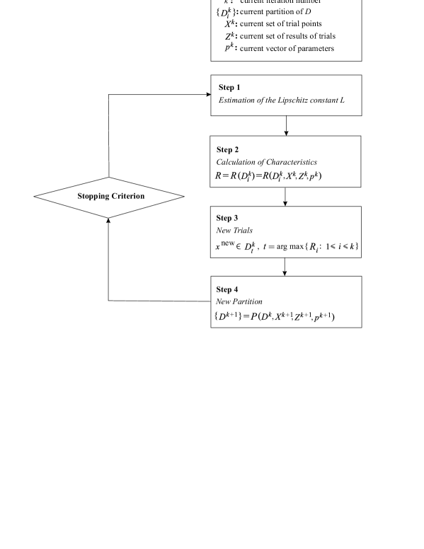
Figure 2: Flow chart of ‘Divide-the-Best’ scheme.

In this scheme (the flow chart of its generic iteration is reported in Figure 2), given a vector $p$ of the method parameters, an adaptive partition of the admissible region $D$ from (5) into a collection $\{D^{k}_{i}\}$ of the finite number of robust subsets $D^{k}_{i}$ is considered at each iteration $k$. The ‘merit’ (called characteristic) $R_{i}$ of each subset (see Step 2 in Figure 2) for performing a subsequent, more detailed, investigation (see Steps 3 and 4 in Figure 2) is estimated on the basis of the obtained information $X^{k}$, $Z^{k}$ about the objective function. The best (in some predefined sense) characteristic obtained over some hyperinterval $D^{k}_{t}$ corresponds to a higher possibility to find the global minimizer within $D^{k}_{t}$ (see Step 3). This hyperinterval is subdivided at the next iteration of the algorithm. Naturally, more than one ‘promising’ hyperinterval can be partitioned at every iteration.

Several strategies (mainly, in the context of the geometric approach) for selection of a subset for further partitioning (see Step 3 in Figure 2) and for performing this partitioning (by means of an operator $P$, see Step 4 in Figure 2 and the next subsection 4.2) are proposed by the authors from a general viewpoint and successfully used for solving practical applications (see, e.g., the references in [72, 73]).

Regarding the stopping criteria, one can constantly check, e.g., the volume of a hyperinterval with the best characteristic or depletion of computing resources such as the maximum number of trials. The verification of a stopping criterion can be performed at any step of the current iteration of the algorithm.

Convergence properties of the ‘Divide-the-Best’ family for different types of characteristic values and partition operators are studied in [72, 67]. Great attention is given to situations (very important in practice) when conditions of global (local) convergence are satisfied not in the whole search domain $D$, but only in its small subregion (or a set of subregions). This can correspond, for example, to Lipschitz global optimization algorithms that work underestimating the Lipschitz constant or which are oriented on using local information in subregions of $D$ (see, e.g., [72, 80, 67]). It should be also noted that the described scheme can be successfully applied to constructing parallel multidimensional global optimization algorithms [80, 24].

4.2 Efficient partitioning strategy

Regarding the partitioning strategies (partitioning operator $P$ on Step 4 in Figure 2), the main attention of the authors is focused on the diagonal partition strategies (see the references in [59, 72, 73, 71]).

In this approach, the initial hyperinterval $D$ from (5) is partitioned into a set of smaller hyperintervals, the objective function is evaluated only at two vertices corresponding to the main diagonal of hyperintervals of the current partition of $D$ (see, e.g., points $a_{i}$ and $b_{i}$ of a hyperinterval $D_{i}$ in Figure 3), and the results of these evaluations are used to select a hyperinterval for the further subdivision. The diagonal approach has a number of attractive theoretical properties and has proved to be efficient in solving applied problems.

Figure 3: Lower bounding a Lipschitz function $f(x)$ over a hyperinterval $D_{i}$ in a diagonal algorithm.

First, it allows one to easily perform an extension of efficient univariate global optimization algorithms to the multidimensional case (see, e.g., [72, 73, 71]). In fact, in order to calculate the characteristic $R_{i}$ of a multidimensional subregion $D_{i}$, some one-dimensional characteristics can be used as prototypes. After an appropriate transformation they can be applied to the one-dimensional segment being the main diagonal $[a_{i},b_{i}]$ of the hyperinterval $D_{i}$ (see Lipschitz-based lower bounding functions $H_{1}$ and $H_{2}$ in Figure 3).

Second, the diagonal approach is close from the computational point of view to one of the simplest strategies—centre-sampling technique (see, e.g., [6, 30, 14, 15, 19])—but at the same time, the objective function is evaluated at two points of each subregion, providing in this way more information about the function over the subregion than centre-sampling methods.

Different exploration techniques based on various diagonal adaptive partition strategies are analyzed, e.g., in [72, 73, 68]. It is demonstrated that partition strategies traditionally used in the framework of the diagonal approach do not fulfil the requirements of computational efficiency because of the execution of many redundant trials. Such a redundancy slows down significantly the global search in the case of costly functions.

An efficient diagonal partition strategy is therefore proposed in [72, 68], that allows one to avoid the computational redundancy of traditional diagonal schemes. In contrast to these schemes, the proposed strategy produces regular meshes of the function evaluation points in such a way that one vertex where $f(x)$ is evaluated can belong to several hyperintervals (up to $2^{N}$, $N$ is the problem dimension from (5)). Thus, the time-consuming procedure of the function evaluations is replaced by a significantly faster operation of reading (up to $2^{N}$ times) the function values obtained at the previous iterations and saved in a special database (see, e.g., [37, 36]). Hence, this partition strategy considerably speeds up the search and also leads to saving computer memory. It is particularly important that these advantages become more pronounced when the problem dimension $N$ increases (see, e.g., [72, 71, 41]).

A novel scheme for creating fast Lipschitz global optimization algorithms is, thus, introduced by the authors. It relies on the efficient diagonal partition strategy allowing an efficient extension of popular one-dimensional Lipschitz global optimization algorithms to the multidimensional case. In a sense, this scheme combines the ideas of the diagonal approach and Peano space-filling curves (see, e.g., [80, 79, 75]). Innovative multidimensional diagonal algorithms for solving Lipschitz global optimization problems, based on different ways for obtaining the Lipschitz information and developed in the framework of the efficient diagonal scheme, are proposed by the authors and their convergence properties are analyzed, e.g., in [72, 71, 41].

4.3 Balancing local and global information

Is well known (see, e.g., [17, 28, 72, 80, 78]) that the usage of the only global information on the objective function and constraints during optimization can lead to a slow convergence of algorithms to global minimizers. Therefore, particular attention is paid by the authors to the usage of local information in global optimization methods, as well. One of the traditional ways in this context (see, e.g., [17, 28, 55]) recommends stopping the global procedure and switching to a local optimization method in order to improve the solution and to accelerate the search during its final phase. Unfortunately, applying this technique can lead to some problems related to the combination of global and local phases, the main problem being that of determining when to stop the global procedure and start the local one. A premature arrest can provoke the loss of the global solution whereas a late one can slow down the search.

Theoretical and experimental results obtained by the authors (see, e.g., [72, 80, 65, 40]) confirm that more fruitful approaches can be considered. The first one is the so-called local tuning approach [65] allowing global optimization algorithms to tune their behaviour to the shape of the functions at different parts of the search domain by estimating the local Lipschitz constants.

In fact, the Lipschitz constant $L$ has a significant influence on the convergence speed of the Lipschitz global optimization algorithms and the problem of its specifying is of great importance. Accepting, for instance, too high a value of $L$ for a concrete objective function means assuming that the function has complicated structure with sharp peaks and narrow attraction regions of minimizers within the whole admissible region. Thus, if the value of $L$ does not correspond to the real behaviour of the objective function, it can lead to a slow convergence of the algorithm to the global minimizer. Global optimization algorithms using in their work a global estimate of $L$ (or some values of $L$ given a priori) do not take into account local information about behaviour of the objective function over every small subregion of $D$. Therefore, estimating local Lipschitz constants allows one to significantly accelerate the global search (see, e.g., [72, 80, 66, 40]).

The second technique regards a continual local improvement of the current best solution incorporated in a global search procedure (see, e.g., [72, 71, 47, 48]). Particularly, it forces the global optimization method to make a local improvement of the best approximation of the global minimum immediately after a new approximation better than the current one is found. These techniques become even more efficient when information about the objective function derivatives is available (see, e.g., [44, 42]).

4.4 Computational aspects

A particular attention is paid by the authors to the problem of testing global optimization algorithms. As widely accepted, a set of test functions is usually taken for this purpose, problems from this set are solved by the algorithms to be compared, and a conclusion about the efficiency of these algorithms is made on the basis of the obtained numerical results. This approach, being an important instrument for acquiring a knowledge about the existing and new global optimization algorithms, presents at the same time some limitations since the conclusions made can be valid only for the selected functions, and their propagation to a more wide set of functions requires particular caution. Testing an algorithm on a relatively large set of test functions can, in a sense, diminish these limitations, but it needs, among other things, the coding of the functions, and it is a tedious and time-consuming job. Moreover, the lack of such information as number of local optima, their locations, attraction regions, local and global values, describing global optimization tests taken from real-life applications, creates additional difficulties in verifying validity of the algorithms. Therefore, the global optimizers are very interested in simple and powerful software tools realizing test problems. As observed, e.g., in [72, 80, 85, 61, 23, 12, 54], a well designed testing framework is of the primary importance in identifying the merits of each algorithm and implementation.

To tackle the problem of testing global optimization algorithms systematically, the GKLS-generator described in [20] is proposed by the authors’ group. The generator produces several classes of multidimensional and multiextremal test functions with known local and global minima. Each test class provided by the generator includes 100 functions. By changing the user-defined parameters, classes with different properties can be created. For example, fixed dimension of the functions and number of local minima, a more difficult class can be created either by shrinking the attraction region of the global minimizer, or by moving the global minimizer closer to the domain boundary.

The generator is available on the ACM Collected Algorithms (CALGO) database (the CALGO is part of a family of publications produced by the Association for Computing Machinery) and it is also downloadable for free from http:\\wwwinfo.dimes.unical.it\~yaro\GKLS.html. It has already been downloaded by companies and research organizations from more than 40 countries of the world.

5 Some numerical results

To conclude, we would like to report some numerical results obtained by using a Lipschitz global optimization method proposed by the authors in [71]. In developing this method for solving problem (3), (5), (6), techniques from the previous Section have been applied. Particularly, it is a multidimensional ‘Divide-the-Best’ global optimization method that uses in its work multiple estimates of the Lipschitz constant and based on efficient diagonal partitions.

Numerical results performed on the GKLS-generator to compare this algorithm with two algorithms belonging to the same class of methods for solving problem (3), (5), (6) — the DIRECT algorithm from [30] and its locally-biased modification DIRECTl  from [19] — are presented here, as described in [71]. As known, both of these methods are widely used in solving practical engineering problems (see, e.g., the references in [17, 34, 71]). Moreover, as shown numerically in [22], they often outperform metaheuristic algorithms as, e.g., the Firefly algorithm (see [83]) belonging to the widely used family of Particle Swarm Optimization algorithms (see, e.g., [83, 82]).

Eight GKLS classes of continuously differentiable test functions of dimensions $N=2$, 3, 4, and 5 have been used. For each dimension, both a ‘hard’ and a ‘simple’ classes have been considered. The difficulty of a class was increased either by decreasing the radius of the attraction region of the global minimizer, or by decreasing the distance from the global minimizer $x^{*}$ to the domain boundaries.

The global minimizer $x^{*}\in D$ was considered to be found when the algorithm generated a trial point $x^{\prime}$ inside a hypercube with a vertex $x^{*}$ and the volume smaller than the volume of the initial hypercube $D=[a,b]$ multiplied by an accuracy coefficient $\Delta$, $0<\Delta\leq 1$, i.e.,

$$|x^{\prime}(j)-x^{*}(j)|\leq\sqrt[N]{\Delta}(b(j)-a(j))$$ (9)

for all $i$, $1\leq j\leq N$, where $N$ is from (5). The algorithm stopped either when the maximal number of trials equal to 1 000 000 was reached, or when condition (9) was satisfied.

In view of the high computational complexity of each trial of the objective function, the methods were compared in terms of the number of evaluations of $f(x)$ required to satisfy condition (9). The number of hyperintervals generated until condition (9) is satisfied, was taken as the second criterion for comparison of the methods. This number reflects indirectly degree of qualitative examination of $D$ during the search for a global minimum (see, e.g., [72, 71, 41]).

Results of numerical experiments with eight GKLS tests classes are reported in Tables 2–2. These tables show, respectively, the maximal number of trials and the corresponding number of generated hyperintervals required for satisfying condition (9) for a half of the functions of a particular class (columns “50%”) and for all 100 function of the class (columns “100%”). The notation “$>$ 1 000 000 $(k)$” means that after 1 000 000 trials the method under consideration was not able to solve $k$ problems.

Note that on a half of test functions from each class (which were simple for each method with respect to the other functions of the class) the algorithm from [71] manifested a good performance with respect to DIRECT and DIRECTl in terms of the number of generated trial points (see Table 2). When all functions were taken in consideration, the number of trials produced by the new algorithm was significantly fewer in comparison with two other methods (see columns “100%” of Table 2), providing at the same time a good examination of the admissible region (see Table 2).

Table 1: Number of trial points for 800 GKLS test functions.

$N$	$\Delta$	Class	50%			100%
			DIRECT	DIRECTl	New	DIRECT	DIRECTl	New
2	$10^{-4}$	simple	111	152	166	1159	2318	403
2	$10^{-4}$	hard	1062	1328	613	3201	3414	1809
3	$10^{-6}$	simple	386	591	615	12507	13309	2506
3	$10^{-6}$	hard	1749	1967	1743	$>$1000000 (4)	29233	6006
4	$10^{-6}$	simple	4805	7194	4098	$>$1000000 (4)	118744	14520
4	$10^{-6}$	hard	16114	33147	15064	$>$1000000 (7)	287857	42649
5	$10^{-7}$	simple	1660	9246	3854	$>$1000000 (1)	178217	33533
5	$10^{-7}$	hard	55092	126304	24616	$>$1000000 (16)	$>$1000000 (4)	93745

Table 2: Number of hyperintervals for 800 GKLS test functions.

$N$	$\Delta$	Class	50%			100%
			DIRECT	DIRECTl	New	DIRECT	DIRECTl	New
2	$10^{-4}$	simple	111	152	269	1159	2318	685
2	$10^{-4}$	hard	1062	1328	1075	3201	3414	3307
3	$10^{-6}$	simple	386	591	1545	12507	13309	6815
3	$10^{-6}$	hard	1749	1967	5005	$>$1000000	29233	17555
4	$10^{-6}$	simple	4805	7194	15145	$>$1000000	118744	73037
4	$10^{-6}$	hard	16114	33147	68111	$>$1000000	287857	211973
5	$10^{-7}$	simple	1660	9246	21377	$>$1000000	178217	206323
5	$10^{-7}$	hard	55092	126304	177927	$>$1000000	$>$1000000	735945

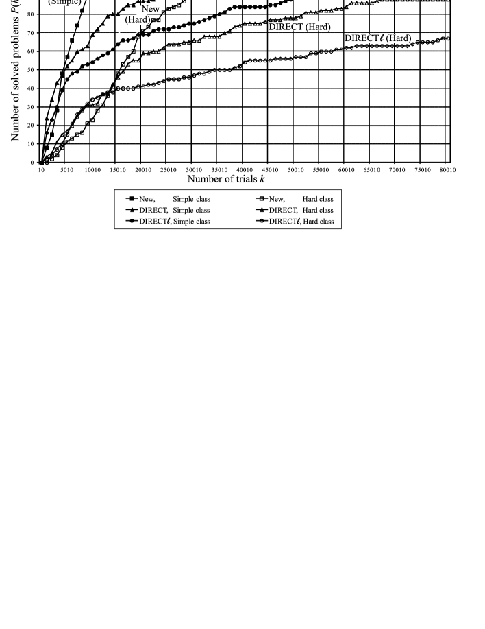
Figure 4: Operating characteristics of the methods New from [71], DIRECT, and DIRECTl on the ‘simple’ and ‘hard’ four-dimensional GKLS test classes

As it can be seen from Tables 2–2, the method [71] demonstrates a quite satisfactory performance with respect to popular DIRECT [30] and DIRECTl [19] methods when multidimensional functions with a really complex structure are minimized. Its superiority can be also confirmed by the so-called operating characteristics (introduced in 1978 in [23], see [80] for their English language description; they can be considered as predecessors of ‘performance profiles’ from [12] and ‘data profiles’ from [54]). The operating characteristics, as an indicator of the efficiency of an optimization method, are formed by the pairs $(k,P(k))$ where $k$ ($k>0$) is the number of trials and $P(k)$ ($0\leq P(k)\leq M$) is the number of test problems (among a set of $M$ tests) solved by the method with less than or equal to $k$ function trials. It is convenient to represent this indicator in a graph where each pair (for increasing values of $k$) corresponds to a point on the plane.

For example, Figure 4 illustrates the operating characteristics for the new method and the DIRECT and DIRECTl methods while solving $M=100$ four-dimensional functions of both ‘simple’ and ‘hard’ GKLS classes. The transition from the ‘simple’ class to the ‘hard’ one can be clearly traced in the diagram: e.g., the new method has solved 50 problems from the ‘simple’ class after 4098 trials while the solution of 50 problems from the ‘hard’ class has required 15064 trials (see the intersection of the horizontal line $P(k)=50$ with graphs labelled ‘New (Simple)’ and ‘New (Hard)’ in Figure 4).

By examining the operating characteristics in Figure 4, it can be seen that for functions with simple structure (up to 50 functions of the ‘simple’ class and up to 40 functions of the ‘hard’ class) all three methods behave similarly. But from the global optimization viewpoint such functions are not interesting because it is possible to successfully minimize them even by very naive methods. The situation is changed when problems with complex structure should be solved: here, both the DIRECT and DIRECTl methods experience serious difficulties. For example, on the ‘hard’ class the new method has solved all 100 problems after about 43000 trials while the DIRECT method has solved 75 problems after the same number of trials and the DIRECTl method — only 55 problems. Note also that even after 80000 trials neither DIRECT nor DIRECTl methods were able to solve all the problems of both the ‘simple’ and ‘hard’ classes of dimension $N=4$ (see the most right vertical line in Figure 4). A similar situation occurs for the operating characteristics on classes of dimensions $N=2$, $3$, and $5$, thus, confirming the efficiency of the proposed method compared with the DIRECT and DIRECTl methods when solving multidimensional multiextremal problems.

This method, as an example of the deterministic techniques mentioned in the previous Sections, not only has manifested a high performance on a large set of tests, but has been also successfully applied for solving real-world global optimization problems. For example, its application to a control theory problem has been considered in [39]. This problem regards global tuning of fuzzy power system stabilizers present in a multi-machine power system in order to damp the power system oscillations. Power system stabilizers with conventional industry structure are extensively used in modern power systems as an efficient means of damping power. Traditionally their parameters are determined by a local tuning procedure based on a single-machine infinite-bus system in which the effects of inter-machine and inter-area dynamics are usually ignored. Heuristic methods (like genetic algorithms) are usually used for their optimizing (as in many other engineering contexts) that often leads to very rough solutions (see, e.g., the references in [39]). To improve overall system dynamic performance, novel global optimization techniques have been therefore applied by the authors’ group in [39].

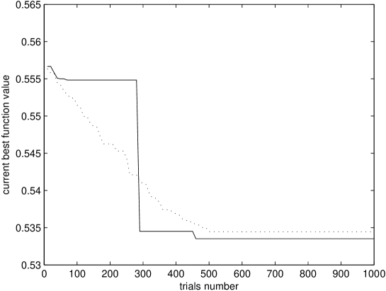
Figure 5: Solutions to the problem of global tuning fuzzy power system stabilizers (see [39]) obtained by applying the method [71] based on the authors’ techniques (solid line) and by a traditionally used genetic approach (dotted line).

In Figure 5, the graph that illustrates the best solution (the axis of ordinates) obtained by a particular genetic algorithm (often used by engineers from the control field) and by the method [71] after a number of simulations (the axis of abscissas) is reported. It can be seen that the global optimization method proposed by the authors spent more function trials (namely, 284 trials) than the genetic algorithm at the initial iterations. This phase corresponds to the initial exploration of the search domain and it is necessary for all global optimization techniques. On the initial phase of the work (less than 300 trials) the genetic algorithm has found local solutions to the problem better than those found by the method [71], but far from the final global solution ($f^{*}\approx 0.533$). However, it is more important and should be underlined that the method [71] has determined a solution to the problem very close to the global optimal one (as demonstrated in [39]) in almost half of the simulations with respect to the genetic algorithm (284 trials for the method [71] and 500 for the genetic algorithm). Moreover, it has found an attraction region of a new minimizer with a much better solution to the problem (see the graph jump in Figure 5 around 450 trials) than that found by the genetic approach. Thus, when a reasonable limit of function trials is given, the considered method [71] can determine a good estimate of the global solution to the studied control theory problem faster than the traditionally used genetic techniques.

Therefore, global optimization techniques briefly presented in this survey can provide the scientists and engineers with comprehensive and powerful tools for successful solving challenging decision-making problems from different real-life application areas, which are characterized by black-box multiextremal and hard to evaluate functions. A more detailed and systematic comparison of the described deterministic approaches with some heuristic nature inspired techniques widely used in engineering applications could be an interesting and useful direction of future research.

References

- [1] C. Audet and J. E. Dennis, Jr. Analysis of generalized pattern searches. SIAM J. Optim., 13(13):889–903, 2003.
- [2] C. Audet and J. E. Dennis, Jr. Mesh adaptive direct search algorithms for constrained optimization. SIAM J. Optim., 17(1):188–217, 2006.
- [3] C. Audet, P. Hansen, and G. Savard, editors. Essays and Surveys in Global Optimization. GERAD 25th Anniversary. Springer, New York, 2005.
- [4] K. A. Barkalov and R. G. Strongin. A global optimization technique with an adaptive order of checking for constraints. Comput. Math. Math. Phys., 42(9):1289–1300, 2002.
- [5] A. J. Booker, J. E. Dennis, Jr., P. D. Frank, D. B. Serafini, V. Torczon, and M. W. Trosset. A rigorous framework for optimization of expensive functions by surrogates. Struct. Optim., 17(1):1–13, 1999.
- [6] A. R. Conn, K. Scheinberg, and L. N. Vicente. Introduction to Derivative-Free Optimization. SIAM, Philadelphia, USA, 2009.
- [7] G. Corliss, C. Faure, A. Griewank, L. Hascoet, and U. Naumann, editors. Automatic Differentiation of Algorithms: From Simulation to Optimization. Springer, New York, 2002.
- [8] T. Csendes, editor. Developments in Reliable Computing. Kluwer Academic Publishers, Dordrecht, 2000.
- [9] A. L. Custódio, J. F. Aguilar Madeira, A. I. F. Vaz, and L. N. Vicente. Direct multisearch for multiobjective optimization. SIAM J. Optim., 21(3):1109–1140, 2011.
- [10] A. L. Custódio and L. N. Vicente. Using sampling and simplex derivatives in pattern search methods. SIAM J. Optim., 18(2):537–555, 2007.
- [11] D. Di Serafino, G. Liuzzi, V. Piccialli, F. Riccio, and G. Toraldo. A modified DIviding RECTangles algorithm for a problem in astrophysics. J. Optim. Theory Appl., 151(1):175–190, 2011.
- [12] E. D. Dolan and J. J. Moré. Benchmarking optimization software with performance profiles. Math. Program., 91:201–213, 2002.
- [13] Yu. G. Evtushenko. Numerical methods for finding global extrema (Case of a non-uniform mesh). USSR Comput. Math. Math. Phys., 11(6):38–54, 1971.
- [14] Yu. G. Evtushenko. Numerical Optimization Techniques. Translations Series in Mathematics and Engineering. Springer–Verlag, Berlin, 1985.
- [15] Yu. G. Evtushenko and M. A. Posypkin. An application of the nonuniform covering method to global optimization of mixed integer nonlinear problems. Comput. Math. Math. Phys., 51(8):1286–1298, 2011.
- [16] C. A. Floudas. Deterministic Global Optimization: Theory, Algorithms, and Applications. Kluwer Academic Publishers, Dordrecht, 2000.
- [17] C. A. Floudas and P. M. Pardalos, editors. Encyclopedia of Optimization (6 Volumes). Springer, 2nd edition, 2009.
- [18] A. I. J. Forrester, A. Sobester, and A. J. Keane. Engineering Design via Surrogate Modelling: A Practical Guide. Wiley, Chichester, USA, 2008.
- [19] J. M. Gablonsky and C. T. Kelley. A locally-biased form of the DIRECT algorithm. J. Global Optim., 21(1):27–37, 2001.
- [20] M. Gaviano, D. E. Kvasov, D. Lera, and Ya. D. Sergeyev. Algorithm 829: Software for generation of classes of test functions with known local and global minima for global optimization. ACM Trans. Math. Software, 29(4):469–480, 2003.
- [21] V. I. Golubev, D. E. Kvasov, and I. E. Kvasov. Identification of seismogeological cracks location by using numerical global optimization methods. In Proc. of the 53rd MIPT Scientific Conference “Recent Advances in Basic and Applied Sciences”, volume VII (2), pages 20–22, Moscow, November 2010. MIPT Press.
- [22] R. Grbić, E. K. Nyarko, and R. Scitovski. A modification of the DIRECT method for Lipschitz global optimization for a symmetric function. J. Global Optim., 57(4):1193–1212, 2013.
- [23] V. A. Grishagin. Operating characteristics of some global search algorithms. In Problems of Stochastic Search, volume 7, pages 198–206. Zinatne, Riga, 1978. In Russian.
- [24] V. A. Grishagin, Ya. D. Sergeyev, and R. G. Strongin. Parallel characteristic algorithms for solving problems of global optimization. J. Global Optim., 10(2):185–206, 1997.
- [25] I. E. Grossmann, editor. Global Optimization in Engineering Design. Kluwer Academic Publishers, Dordrecht, 1996.
- [26] N. Hansen and A. Ostermeier. Completely derandomized self-adaptation in evolution strategies. Evolut. Comput., 9(2):159–195, 2001.
- [27] J. H. Holland. Adaptation in Natural and Artificial Systems. The University of Michigan Press, Ann Arbor, USA, 1975.
- [28] R. Horst and P. M. Pardalos, editors. Handbook of Global Optimization, volume 1. Kluwer Academic Publishers, Dordrecht, 1995.
- [29] D. R. Jones. A taxonomy of global optimization methods based on response surfaces. J. Global Optim., 21(4):345–383, 2001.
- [30] D. R. Jones, C. D. Perttunen, and B. E. Stuckman. Lipschitzian optimization without the Lipschitz constant. J. Optim. Theory Appl., 79(1):157–181, 1993.
- [31] D. R. Jones, M. Schonlau, and W. J. Welch. Efficient global optimization of expensive black-box functions. J. Global Optim., 13(4):455–492, 1998.
- [32] D. Karaboga and B. Akay. A comparative study of Artificial Bee Colony algorithm. Appl. Math. Comput., 214:108–132, 2009.
- [33] R. B. Kearfott. Rigorous Global Search: Continuous Problems. Kluwer Academic Publishers, Dordrecht, 1996.
- [34] C. T. Kelley. Iterative Methods for Optimization. SIAM Publications, Philadelphia, 1999.
- [35] T. G. Kolda, R. M. Lewis, and V. Torczon. Optimization by direct search: New perspectives on some classical and modern methods. SIAM Rev., 45(3):385–482, 2003.
- [36] D. E. Kvasov. Diagonal numerical methods for solving lipschitz global optimization problems. Bollettino U.M.I., I (Serie IX)(3):857–871, 2008.
- [37] D. E. Kvasov. Multidimensional Lipschitz global optimization based on efficient diagonal partitions. 4OR – Quart. J. Oper. Res., 6(4):403–406, 2008.
- [38] D. E. Kvasov, I. E. Kvasov, and M. V. Muratov. The study of an inverse problem of fractured reservoir modeling by using numerical global optimization methods. In Proc. of the 55th MIPT Scientific Conference “Recent Advances in Basic and Applied Sciences”, volume 2, pages 135–136, Moscow, November 2012. MIPT Press.
- [39] D. E. Kvasov, D. Menniti, A. Pinnarelli, Ya. D. Sergeyev, and N. Sorrentino. Tuning fuzzy power-system stabilizers in multi-machine systems by global optimization algorithms based on efficient domain partitions. Electr. Power Syst. Res., 78(7):1217–1229, 2008.
- [40] D. E. Kvasov, C. Pizzuti, and Ya. D. Sergeyev. Local tuning and partition strategies for diagonal GO methods. Numer. Math., 94(1):93–106, 2003.
- [41] D. E. Kvasov and Ya. D. Sergeyev. Multidimensional global optimization algorithm based on adaptive diagonal curves. Comput. Math. Math. Phys., 43(1):40–56, 2003.
- [42] D. E. Kvasov and Ya. D. Sergeyev. A univariate global search working with a set of Lipschitz constants for the first derivative. Optim. Lett., 3(2):303–318, 2009.
- [43] D. E. Kvasov and Ya. D. Sergeyev. Deterministic gobal optimization methods for solving engineering problems. In B. H. V. Topping, editor, Proceedings of the Eleventh International Conference on Computational Structures Technology, page 62, Stirlingshire, United Kingdom, 2012. Civil-Comp Press. doi: 10.4203/ccp.99.62.
- [44] D. E. Kvasov and Ya. D. Sergeyev. Lipschitz gradients for global optimization in a one-point-based partitioning scheme. J. Comput. Appl. Math., 236(16):4042–4054, 2012.
- [45] D. E. Kvasov and Ya. D. Sergeyev. Univariate geometric Lipschitz global optimization algorithms. Numer. Algebra Contr. Optim., 2(1):69–90, 2012.
- [46] I. E. Kvasov and I. B. Petrov. High-performance computer simulation of wave processes in geological media in seismic exploration. Comput. Math. Math. Phys., 52(2):302–313, 2012.
- [47] D. Lera and Ya. D. Sergeyev. An information global minimization algorithm using the local improvement technique. J. Global Optim., 48(1):99–112, 2010.
- [48] D. Lera and Ya. D. Sergeyev. Acceleration of univariate global optimization algorithms working with Lipschitz functions and Lipschitz first derivatives. SIAM J. Optim., 23(1):508–529, 2013.
- [49] V. B. Leviant, I. B. Petrov, F. B. Chelnokov, and I. Y. Antonova. Nature of the scattered seismic response from zones of random clusters of cavities and fractures in a massive rock. Geophysical Prospecting, 55(4):507–524, 2007.
- [50] G. Liuzzi, S. Lucidi, and M. Sciandrone. Sequential penalty derivative-free methods for nonlinear constrained optimization. SIAM J. Optim., 20(5):2614–2635, 2010.
- [51] L. Ljung. System Identification: Theory for the User. PTR Prentice Hall, Upper Saddle River, N.J., 2nd edition, 1999.
- [52] Z. Michalewicz. Genetic Algorithms + Data Structures = Evolution Programs. Springer–Verlag, Berlin, 3rd edition, 1996.
- [53] J. Mockus. A Set of Examples of Global and Discrete Optimization: Applications of Bayesian Heuristic Approach. Kluwer Academic Publishers, Dordrecht, 2000.
- [54] J. J. Moré and S. M. Wild. Benchmarking derivative-free optimization algorithms. SIAM J. Optim., 20(1):172–191, 2009.
- [55] P. M. Pardalos and H. E. Romeijn, editors. Handbook of Global Optimization, volume 2. Kluwer Academic Publishers, Dordrecht, 2002.
- [56] R. Paulavičius and J. Žilinskas. Simplicial Global Optimization. Springer, New York, 2014.
- [57] R. Paulavičius and J. Žilinskas. Simplicial Lipschitz optimization without the Lipschitz constant. J. Global Optim., 59(1):23–40, 2014.
- [58] I. B. Petrov and A. S. Kholodov. Numerical investigation of certain dynamical problems of the mechanics of a deformable solid body by the grid-characteristic method. USSR Comput. Math. Math. Phys., 24(3):61–73, 1984.
- [59] J. D. Pintér. Global Optimization in Action (Continuous and Lipschitz Optimization: Algorithms, Implementations and Applications). Kluwer Academic Publishers, Dordrecht, 1996.
- [60] R. G. Regis and C. A. Shoemaker. Constrained global optimization of expensive black box functions using radial basis functions. J. Global Optim., 31(1):153–171, 2005.
- [61] L. M. Rios and N. V. Sahinidis. Derivative-free optimization: A review of algorithms and comparison of software implementations. J. Global Optim., 56:1247–1293, 2013.
- [62] K. Schittkowski. Numerical Data Fitting in Dynamical Systems: A Practical Introduction with Applications and Software. Kluwer Academic Publishers, Dordrecht, 2002.
- [63] J. J. Schneider and S. Kirkpatrick. Stochastic Optimization. Springer, Berlin, 2006.
- [64] M. K. Sen and P. L. Stoffa. Global Optimization Methods in Geophysical Inversion. Elsevier Science B.V., Amsterdam, 1995.
- [65] Ya. D. Sergeyev. An information global optimization algorithm with local tuning. SIAM J. Optim., 5(4):858–870, 1995.
- [66] Ya. D. Sergeyev. Global one-dimensional optimization using smooth auxiliary functions. Math. Program., 81(1):127–146, 1998.
- [67] Ya. D. Sergeyev. On convergence of “Divide the Best” global optimization algorithms. Optimization, 44(3):303–325, 1998.
- [68] Ya. D. Sergeyev. An efficient strategy for adaptive partition of -dimensional intervals in the framework of diagonal algorithms. J. Optim. Theory Appl., 107(1):145–168, 2000.
- [69] Ya. D. Sergeyev, P. Daponte, D. Grimaldi, and A. Molinaro. Two methods for solving optimization problems arising in electronic measurements and electrical engineering. SIAM J. Optim., 10(1):1–21, 1999.
- [70] Ya. D. Sergeyev, D. Famularo, and P. Pugliese. Index branch-and-bound algorithm for Lipschitz univariate global optimization with multiextremal constraints. J. Global Optim., 21(3):317–341, 2001.
- [71] Ya. D. Sergeyev and D. E. Kvasov. Global search based on efficient diagonal partitions and a set of Lipschitz constants. SIAM J. Optim., 16(3):910–937, 2006.
- [72] Ya. D. Sergeyev and D. E. Kvasov. Diagonal Global Optimization Methods. FizMatLit, Moscow, 2008. In Russian.
- [73] Ya. D. Sergeyev and D. E. Kvasov. Lipschitz global optimization. In J. J. Cochran, editor, Wiley Encyclopedia of Operations Research and Management Science, volume 4, pages 2812–2828. Wiley, New York, 2011.
- [74] Ya. D. Sergeyev, D. E. Kvasov, and F. M. H. Khalaf. A one-dimensional local tuning algorithm for solving GO problems with partially defined constraints. Optim. Lett., 1(1):85–99, 2007.
- [75] Ya. D. Sergeyev, R. G. Strongin, and D. Lera. Introduction to Global Optimization Exploiting Space-Filling Curves. Springer, New York, 2013.
- [76] S. Shan and G. G. Wang. Survey of modeling and optimization strategies to solve high-dimensional design problems with computationally-expensive black-box functions. Struct. Multidiscipl. Optim., 41(2):219–241, 2010.
- [77] G. E. Stavroulakis. Inverse and Crack Identification Problems in Engineering Mechanics. Kluwer Academic Publishers, Dordrecht, 2001.
- [78] C. P. Stephens and W. Baritompa. Global optimization requires global information. J. Optim. Theory Appl., 96(3):575–588, 1998.
- [79] R. G. Strongin. Numerical Methods in Multiextremal Problems (Information-Statistical Algorithms). Nauka, Moscow, 1978. In Russian.
- [80] R. G. Strongin and Ya. D. Sergeyev. Global Optimization with Non-Convex Constraints: Sequential and Parallel Algorithms. Kluwer Academic Publishers, Dordrecht, 2000.
- [81] V. Torczon. On the convergence of pattern search algorithms. SIAM J. Optim., 7(1):1–25, 1997.
- [82] A. I. F. Vaz and L. N. Vicente. A particle swarm pattern search method for bound constrained global optimization. J. Global Optim., 39:197–219, 2007.
- [83] X.-S. Yang. Engineering Optimization: An Introduction with Metaheuristic Applications. Wiley, USA, 2010.
- [84] A. A. Zhigljavsky. Theory of Global Random Search. Kluwer Academic Publishers, Dordrecht, 1991.
- [85] A. A. Zhigljavsky and A. Žilinskas. Stochastic Global Optimization. Springer, New York, 2008.