Solving constrained quadratic binary problems
via quantum adiabatic evolution

Abstract.

Quantum adiabatic evolution is perceived as useful for binary quadratic programming problems that are a priori unconstrained. For constrained problems, it is a common practice to relax linear equality constraints as penalty terms in the objective function. However, there has not yet been proposed a method for efficiently dealing with inequality constraints using the quantum adiabatic approach. In this paper, we give a method for solving the Lagrangian dual of a binary quadratic programming (BQP) problem in the presence of inequality constraints and employ this procedure within a branch-and-bound framework for constrained BQP (CBQP) problems.

1. Introduction

An unconstrained binary quadratic programming (UBQP) problem is defined by

(1) Minimize $$x^{T}Qx$$

subject to $$x\in\{0,1\}^{n},$$

where, without loss of generality, $Q\in\mathbb{Z}^{n\times n}$. Recent advancements in quantum computing technology [10, 28, 31] have raised hopes of the production of computing systems that are capable of solving UBQP problems, and showing quantum speedup. The stochastic nature of such systems, together with extant sources of noise and error, are challenges yet to be overcome in achieving scalable quantum computing systems of this type. This paper is nevertheless motivated by the assumption of the existence of systems that can solve UBQP problems efficiently and to optimality, or at least in conjunction with a framework of noise analysis of the suboptimal results. We call such a computing system a UBQP oracle.

Many NP-hard combinatorial optimization problems arise naturally or can easily be reformulated as UBQP problems, such as the quadratic assignment problem, the maximum cut problem, the maximum clique problem, the set packing problem, and the graph colouring problem (see, for instance, Boros and Prékopa [14], Boros and Hammer [12], Bourjolly et al. [15], Du and Pardalos [20], Pardalos and Rodgers [40, 41], Pardalos and Xue [42], and Kochenberger et al. [33]).

Numerous interesting applications that are expressed naturally in the form of UBQP problems appear in the literature. Barahona et al. [7, 19] formulate and solve the problem of finding exact ground states of spin glasses with magnetic fields. Alidaee et al. [4] study the problem of scheduling $n$ jobs non-preemptively on two parallel identical processors to minimize weighted mean flow time as a UBQP problem. Bomze et al. [11] give a comprehensive discussion of the maximum clique (MC) problem. Included is the UBQP representation of the MC problem and a variety of applications from different domains. UBQP has been used in the prediction of epileptic seizures [27]. Alidaee et al. [3] discuss a number partitioning problem, formulating a special case as a UBQP problem.

In this paper, we consider constrained binary quadratic programming (CBQP) problems with linear constraints, stated formally as

(2) $$\mathrm{(P)} x^{T}Qx$$ Minimize

subject to $$Ax\leq b,$$

$$x\in\{0,1\}^{n}\,,$$

where $Q\in\mathbb{Z}^{n\times n}$ and $A\in\mathbb{Z}^{m\times n}$.

There are many problems which naturally occur as linearly constrained binary quadratic programming problems. To illustrate, consider the well-studied quadratic assignment problem: the problem of assigning facilities to locations where the cost is a function of the distance and flow between facilities plus the cost of assigning a facility to a specific location. The problem requires that each facility be assigned exactly one location, and each location exactly one facility, and is easily expressed in the form of (P) [34]. Other examples include the clique partitioning problem [39], the quadratic minimum spanning tree problem [6], and the quadratic shortest path problem [45].

In the literature, CBQP problems are commonly reformulated as UBQP problems by including quadratic penalties in the objective function as an alternative to explicitly imposing constraints. Although this method has been used very successfully on classical hardware, it is not a viable approach when using quantum adiabatic hardware, as the reformulation dramatically increases the density, range of coefficients, and dimension of the problem.

We present a branch-and-bound approach which uses Lagrangian duality to solve (P) and show that a UBQP oracle can be used to solve the Lagrangian dual (LD) problem with successive applications of linear programming (LP). Throughout this paper, we will refer to this algorithm as the quantum branch-and-bound algorithm. We introduce the notion of quantum annealing leniency, which can be used to compare a classical algorithm running on a Turing machine to an algorithm running on an oracle Turing machine [47] with a quantum annealing oracle. This measure represents the maximum threshold of the average time an oracle query is allowed to take in order to outperform the benchmark algorithm running on a classical Turing machine. In our experiments, we benchmark our quantum branch-and-bound algorithm against the Gurobi Optimizer [24]. The quantum annealing leniency of the quantum branch-and-bound algorithm with respect to the Gurobi Optimizer is measured.

This paper is organized as follows. Section 2 gives an overview of the quantum adiabatic approach to computation and the relationship of the approach to UBQP. Section 3 presents lower- bounding procedures for CBQP. Section 4 presents a local search heuristic for CBQP. Branching strategies are described in Section 5. All of these algorithms are then integrated in the quantum branch-and-bound framework presented in Section 6. Test instances and results of our computational experiments are presented in Section 7. In Section 8, we provide practical instruction for the application of our method to the quantum processors manufactured by D-Wave Systems Inc., and in Section 9, we mention how our method can more generally be used to solve constrained binary programming problems with higher-order polynomial objectives and higher-order polynomial constraints.

2. Computing using quantum adiabatic evolution

Recent advancements in quantum hardware technology have motivated an increase in the study of forms of computation that differ in computational complexity from Turing machines. The quantum gate model is a means of achieving powerful quantum algorithms such as Shor’s well known quantum algorithms for integer factorization and computing discrete logarithms [46]. Aside from the quantum gate model, there are several other paradigms of quantum information technology, each of which would open a new world of possible algorithm designs to be realized on a corresponding practical quantum processor.

Farhi et al. [21, 22] propose quantum adiabatic evolution as a novel paradigm for the design of quantum algorithms. Quantum adiabatic computation is expressed by the Schrödinger equation of a time-dependent Hamiltonian

(3) $$H(t) := \left(1-\mbox{$\frac{t}{T}$}\right)H_{0}+\mbox{$\frac{t}{T}$}H_{f},\quad 0\leq t\leq T\,.$$

Here $T$ is a constant delay factor. The system is evolved according to (3) from an initial Hamiltonian $H_{0}$ at time $t=0$ to a final Hamiltonian $H_{f}$ at time $t=T$. The former Hamiltonian is such that setting the system to its ground state is easy, and the latter Hamiltonian is constructed from a polynomial objective function $f(z)$ in binary variables. $H_{f}$ is associated to $f$ such that the range of $f$ is identical to the eigenvalue spectrum of $H_{f}$. By the quantum adiabatic theorem [38], when the system is initially set to the ground state of $H_{0}$ at time $t=0$, and $T$ is sufficiently large, the system tends to stay in the ground state of $H(t)$ for all $t$.

Van Dam et al. [48] show that it is sufficient to have $T\in O({\Delta_{\mathrm{max}}}/{g_{\mathrm{min}}^{2}}).$ Here $g_{\mathrm{min}}$ is the minimum difference over time $s$ between the smallest two eigenvalues of $H(s)$ and $\Delta_{\mathrm{max}}:=\max_{s}{\|{\mbox{$\frac{d}{ds}$}}H(s)\|_{2}}$. They give an example of an adiabatic quantum algorithm for searching that matches the quadratic speedup obtained by Grover’s search algorithm. This example demonstrates that the “quantum local search,” which is implicit in the adiabatic evolution, is truly non-classical in nature from a computational perspective. Also [48, Theorem 1] explains how the continuous-time evolution of $t\in[0,T]$ can be approximated by a quantum circuit consisting of a sequence of $\mathrm{poly}(nT)$ unitary transformations.

All of the above considerations suggest that practical quantum hardware can yield a significant quantum speedup in certain integer programming problems. Our goal is to design and analyze optimization algorithms that work in conjunction with such integer programming oracles. Specifically, we work under the assumption of the existence of a UBQP oracle, an oracle Turing machine for solving UBQP problems. This assumption is motivated by prototypes of quantum annealers recently manufactured by D-Wave Systems, where couplings connect pairs of quantum bits [28]. Our suggested methods are easily generalizable to take advantage of systems with higher-degree interactions of quantum bits if such systems are implemented in the future (see Section 9).

As a final remark, it is important to mention that quantum annealers are coupled to an environment, and this significantly affects their performance. Albash et al. [2] propose a noise model for D-Wave devices. This model includes the control noise on the local field and couplings of the chip, as well as the effect of the cross-talk between qubits that are not coupled. Eventually [2] concludes that despite the thermal excitations and small value of the ratio of the single-qubit decoherence time to the annealing time, an open-system, quantum-dynamical description of the D-Wave device that starts from a quantized energy level structure is well justified. The design of benchmark instances that can detect quantum speedup or any quantum advantage of a quantum annealer in comparison to state-of-the-art classical algorithms is studied by Katzgraber et al. [30]. Zhu et al. [50] show that increasing the classical energy gap beyond the intrinsic noise level of the machine can improve the success of the D-Wave Two quantum annealer, at the cost of producing considerably easier benchmark instances. We refer the reader to [32] for the practicality and best practices in using D-Wave devices.

3. Lower-bounding procedures

3.1. Linearization relaxation

A standard linearization of (P) involves relaxing the integrality constraint on variables $x_{i},(i=1,\ldots,n)$, and defining continuous variables $y_{ij}$ for every pair $x_{i}x_{j}$ in the objective function with $i<j$, yielding the following linearized problem.

(4) $$\mathrm{(P_{LP})} \sum\limits_{1\leq i<j\leq n}2\,q_{ij}y_{ij}+\sum_{i=1}^{n}q_{ii}x_{i}$$ Minimize

subject to $$Ax\leq b\,,$$

$$y_{ij}\geq x_{i}+x_{j}-1\quad(\forall\,i,j\text{ such that }i<j\text{ and }q_{ij}>0)\,,$$

$$y_{ij}\leq x_{i}\quad(\forall\,i,j\text{ such that }i<j\text{ and }q_{ij}<0)\,,$$

$$y_{ij}\leq x_{j}\quad(\forall\,i,j\text{ such that }i<j\text{ and }q_{ij}<0)\,,$$

$$0\leq x_{i}\leq 1\quad(i=1,\ldots,n)\,,$$

$$y\geq 0$$

A lower bound to (P) can now be obtained by solving $\mathrm{(P_{LP})}$ using linear programming. We employed this linearization in our computational experiments (see Section 7). Note that there are several methods for linearizing (P), many of which have been mentioned in the survey by Floudas and Gounaris [23]; in this paper, however, we consider $\mathrm{(P_{LP})}$ to be the LP relaxation of (P).

3.2. Lagrangian dual

We can give a lower bound for (P) via the LD problem

(5) $$\mathrm{(L)} \max\limits_{\lambda\in\mathbb{R}^{m}_{+}} d(\lambda)\,,$$

where $d(\lambda)$ is evaluated via the Lagrangian relaxation

(6) $$\mathrm{(L_{\lambda})} d(\lambda)=\min\limits_{x\in\{0,1\}^{n}}L(x,\lambda)= x^{T}Qx+\lambda^{T}(Ax-b)\,.$$

The function $d(\lambda)$ is the minimum of a finite set of linear functions of $\lambda$ and hence it is concave and piecewise linear. The following theorem shows that $\mathrm{L_{\lambda}}$ is a lower bound for (P). For any problem $Q$, let $v(Q)$ be the optimal objective value.

Proposition 1 (Weak Duality): For all $\lambda\in\mathbb{R}^{m}_{+}$, we have $v(L_{\lambda})\leq v(P)\,.$

Proof: Since every feasible solution for (P) is feasible for $L_{\lambda}$, then for any $\lambda\in\mathbb{R}^{m}_{+}$ we have

(7) $$v(P)=\min\limits_{x\in\{0,1\}^{n}}\{x^{T}Qx|Ax\leq b\}\geq\min\limits_{x\in\{0,1\}^{n}}\{x^{T}Qx+\lambda^{T}(Ax-b)\}=v(L_{\lambda})\,.\quad\square\,$$

A number of techniques to solve (L) exist in the literature; however, finding this bound is computationally expensive, so looser bounds (for example, the LP relaxation) are typically used. Note that the problem yields a natural solution using the UBQP oracle via the outer Lagrangian linearization method. The book by Li and Sun [36] provides background and several details of this approach in Procedure 3.2.

Recall that (L) can be rewritten as an LP problem in terms of the real variables $\lambda$ and $\mu$:

(8) $$\mathrm{(L_{LP})} \mu$$ Maximize

subject to $$\mu\leq x^{T}Qx+\lambda^{T}(Ax-b)\quad(\forall x\in\{0,1\}^{n})\,,$$

$$\lambda\geq 0\,.$$

This formulation is difficult to solve directly, as there are an exponential number of constraints. In particular, there is one linear constraint (cutting plane) for every binary point $x\in\{0,1\}^{n}$. However, the restriction of the constraints to a much smaller nonempty subset $T\subseteq\{0,1\}^{n}$ of binary vectors is a tractable LP problem:

(9) $$\mathrm{(L_{LP-T})} \mu$$ Maximize

subject to $$\mu\leq x^{T}Qx+\lambda^{T}(Ax-b)\quad(\forall x\in T)\,,$$

$$\lambda\geq 0\,.$$

This LP problem is bounded provided that $T$ contains at least one feasible solution. In some cases, finding at least one feasible solution can be very difficult. In these cases, we impose an upper bound on the vector of Lagrange multipliers, substituting the constraint $\lambda\geq 0$ by $0\leq\lambda\leq u$.

(10) $$\mathrm{(L_{LP-T}^{u})} \mu$$ Maximize

subject to $$\mu\leq x^{T}Qx+\lambda^{T}(Ax-b)\quad(\forall x\in T)\,,$$

$$0\leq\lambda\leq u$$

The vector $u$ of upper bounds may depend on an estimation of the solution to (L). In practical situations, it should also depend on the specifics of the UBQP oracle (for example, the noise and precision of the oracle). Let $(\mu^{\ast},\lambda^{\ast})$ be an optimal solution to $\mathrm{(L_{LP-T})}$. Note that imposing the box constraint $0\leq\lambda\leq u$ might result in not generating an optimal primal-dual pair, but nevertheless $\mathrm{(L_{LP-T}^{u})}$ generates a lower bound for $\mathrm{(P)}$. It is clear that $(\mathrm{L_{\lambda^{\ast}}})$ is a UBQP problem that can be solved using the UBQP oracle. By successively adding the solutions returned by the UBQP oracle as cutting planes and applying the simplex method, we are able to solve $\mathrm{(L_{LP})}$ (see Algorithm 1).

Algorithm 1 Outer Lagrangian linearization

1:problem $(P)$; initial Lagrange multipliers $\lambda^{*}$

2:optimal primal $x^{*}$; optimal dual solution $(\lambda^{*},\mu^{*})$; a strong-duality flag

3:initialize $\mu^{*}=\infty$, $T=\emptyset$

4:solve $\mathrm{L_{\lambda^{*}}}$, obtain the dual value $d(\lambda^{*})$ and optimal solution $x^{*}\subseteq\{0,1\}^{n}$

5:if $(\lambda^{*})^{T}[A(x^{*})-b]=0$ and $A(x^{*})\leq b$ then

6:     stop and return $x^{*}$ and $(\lambda^{*},d(\lambda^{*}))$, with strong-duality flag set to true

7:if $(\mu^{*})\leq d(\lambda^{*})$ then

8:     stop and return $x^{*}$ and $(\lambda^{*},\mu^{*})$

9:update $T$ by adding $x^{*}$, $T\leftarrow T\cup\{x^{*}\}$

10:solve $L_{LP-T}^{u}$ and update $\mu^{*}$ and $\lambda^{*}$

11:go to step 2

4. A local search heuristic

In order to prune a branch-and-bound tree effectively, it is important to quickly obtain a good upper bound. We employ an adaptation of the local search algorithm presented by Bertsimas et al. [9]. The main idea is as follows: beginning with a feasible solution $x$, the solution is iteratively improved by considering solutions in the 1-flip neighbourhood of $x$ (defined as the set of solutions that can be obtained by flipping a single element of $x$) which are feasible, together with “interesting” solutions, until it cannot be improved further. The algorithm takes a parameter $\rho$ which explicitly controls the trade-off between complexity and performance by increasing the size of the neighbourhood. A neighbouring solution $y$ is considered “interesting” if it satisfies the following conditions: (i) no constraint is violated by more than one unit; and (ii) the number of violated constraints in $y$ plus the number of loose constraints which differ from the loose constraints in the current best solution is at most $\rho$.

Algorithm 2 Local search heuristic (LSH)

1:matrices $A$ and $Q$; vector $b$; feasible solution $z_{0}$; scalar parameter $\rho>0$

2:feasible solution $z$ such that $z^{T}Qz\leq z_{0}^{T}Qz_{0}$

3:$z:=z_{0}$; $S:=\{z\}$

4:while $S\neq\emptyset$ do

5:     get a new solution $x$ from $S$

6:     for all $y$ adjacent to $x$ do

7:         if $y$ is feasible and $y^{T}Qy<z^{T}Qz$ then

8:              $z\leftarrow y$ and $S\leftarrow y$

9:              go to step 3

10:         else if $y$ is interesting then

11:              $S\leftarrow S\cup\{y\}$               

Note that the algorithm moves to a better solution as soon as it finds a feasible one, and only when no solutions are found does it consider moving to “interesting” solutions.

5. Branching strategies

In any branch-and-bound scheme, the performance of the algorithm is largely dependent on the number of nodes that are visited in the search tree. As such, it is important to make effective branching decisions, reducing the size of the search tree. Branching heuristics are usually classified as either static variable-ordering (SVO) heuristics or dynamic variable-ordering (DVO) heuristics. All branching heuristics used in this paper are DVO heuristics, as they are generally considered more effective because they allow information obtained during a search to be utilized to guide the search.

It is often quite difficult to find an assignment of values to variables that satisfies all constraints. This has motivated the study of a variety of approaches that attempt to exploit the interplay between variable-value assignments and constraints. Examples include the impact-based heuristics proposed by Refalo [44], the conflict-driven variable-ordering heuristic proposed by Boussemart et al. [16], and the approximated counting-based heuristics proposed by Kask et al. [29], Hsu et al. [26], Bras et al. [35], and Pesant et al. [43].

5.1. Counting the solution density

One branching heuristic used in this paper is a modified implementation of the maxSD heuristic introduced by Pesant et al. [43]. We recall two definitions.

Definition 5.1.

Given a constraint $c(x_{1},\dots,x_{n})$ and respective finite domains $D_{i}$ $(1\leq i\leq n)$, let $\#c(x_{1},\ldots,x_{n})$ denote the number of $n$-tuples in the corresponding relation.

Definition 5.2.

Given a constraint $c(x_{1},\dots,x_{n})$, respective finite domains $D_{i}$ $(1\leq i\leq n)$, a variable $x_{i}$ in the scope of $c$, and a value $d\in D_{i}$, the solution density of a pair $(x_{i},d)$ in $c$ is given by

(11) $$\sigma(x_{i},d,c)=\frac{\#c(x_{1},\ldots,x_{i-1},d,x_{i+1},\ldots,x_{n})}{\#c(x_{1},\ldots,x_{n})}\,.$$

The solution density measures how frequently a certain assignment of a value in the domain of a variable belongs to a solution that satisfies constraint $c$.

The heuristic maxSD iterates over all of the variable-value pairs and chooses the pair that has the highest solution density. If the (approximate) $\sigma(x_{i},d,c)$ are precomputed, the complexity of the modified algorithm is $O(mq)$, where $m$ is the number of constraints, and $q$ is the sum of the number of variables that appear in each constraint. Pesant et al. [43] detail good approximations of the solution densities for knapsack constraints, which can be computed efficiently. They also provide an in-depth experimental analysis that shows that this heuristic is state of the art among counting-based heuristics.

5.2. Constraint satisfaction via an LD solution

In each node $u$ of the branch-and-bound tree, a lower bound is computed by solving the LD problem $\mathrm{(L)}$, and the primal-dual pair $(x^{u},\lambda^{u})$ is obtained. In the standard way, we define the slack of constraint $i$ at a point $x$ as $s_{i}=b_{i}-a_{i}^{T}x$, where $a_{i}$ is the $i$-th row of $A$. Then the set of violated constraints at $x$ is the set $V=\{i:s_{i}<0\}$. If $x^{u}$ is infeasible for the original problem, it must violate one or more constraints. Additionally, we define the change in slack for constraint $i$ resulting from flipping variable $j$ in $x^{u}$ as

(12) $$\delta_{ij}=a_{ij}(2x^{u}_{j}-1)\,.$$

We present two branching strategies which use this information at $x^{u}$ to guide variable and value selection towards feasibility.

The first branching method we propose is to select the variable that maximizes the reduction in violation of the most violated constraint. That is, we select $j=\operatorname*{arg\,max}\limits_{j\in 1,\dots n}\delta_{ij}$ and value $1-x^{u}_{j}$ (see Algorithm 3).

Algorithm 3 Most-violated-constraint satisfaction branching scheme

1:$x^{u}$ is the optimal solution to (L) at the current node.

2:for all constraints $i$ do

3:     compute $s_{i}=b_{i}-a^{T}_{i}x^{u}$

4:$i=\operatorname*{arg\,min}\limits_{i\in\{1,\ldots,m\}}s_{i}$

5:if $s_{i}>0$ then

6:     LD optimal is feasible; abort violation branching

7:for all variables $j$ do

8:     compute $\delta_{ij}=a_{ij}(2x^{u}_{j}-1)$

9:return index $j=\operatorname*{arg\,max}\limits_{j\in 1,\dots,n}\delta_{ij}$ and value $1-x^{u}_{j}$

The next branching method we discuss is more general: instead of looking only at the most violated constraint, we consider all of the violated constraints and select the variable which, when flipped in the LD solution, gives the maximum decrease in the left-hand side of all violated constraints (see Algorithm 4).

Algorithm 4 All-violated-constraints satisfaction branching scheme

1:$x^{u}$ is the optimal solution to (L) at the current node.

2:for all constraints $i$ do

3:     compute $s_{i}=b_{i}-a^{T}_{i}x^{u}$

4:$V:=\{i:s_{i}<0\}$ defines the set of violated constraints.

5:if $V=\emptyset$ then

6:     LD optimal is feasible; abort violation branching

7:for all variables $j$ do

8:     compute $\delta_{ij}=a_{ij}(2x^{u}_{j}-1)$

9:return index $j=\operatorname*{arg\,max}\limits_{j\in 1,\dots,n}\left(\sum_{i\in V}\delta_{ij}\right)$ and value $1-x^{u}_{j}$

5.3. Pseudo-cost branching

Introduced in CPLEX 7.5 [5], the idea of strong branching is to test which fractional variable gives the best bound before branching. The test is performed by temporarily fixing each fractional variable to 0 or 1 and solving the LP relaxation by the dual simplex method. Since the cost of solving several LP subproblems is high, only a fixed number of iterations of the dual simplex algorithm are performed. The variable fixation that provides the strongest bound is chosen as the branching decision.

If the number of fractional variables is large, this process is very time consuming. There are several possible methods to overcome this difficulty. One way is to select a subset of variables, for example, choosing variables with values close to 0.5. Another approach, the $k$-look-ahead branching strategy, requires an integer parameter $k$ and a score assignment on the fractional variable fixations. The variable fixations are then sorted according to their scores, and the above test is performed. If no better bound is found for $k$ successive variable fixations, the test process is stopped.

The sorting of the variable fixations is only applied in later stages of the branch-and-bound process. We use pseudo-costs, which are introduced in [8] and explained in Section 5.3.1, as the score of a variable fixation.

Note that the lower-bound computation by the UBQP oracle can be performed in parallel with either strong branching or the $k$-look-ahead strategy using a digital processor, affording the computational time required to utilize this type of branching without significantly increasing the total running time of the algorithm.

5.3.1. Pseudo-costs

Pseudo-costs keep track of the success of the variable fixations that have already been used in the branch-and-bound process. Different variations of pseudo-costs have been proposed in the literature. We employ the variation discussed in [1, 37]. Let $f_{i}^{+}$ and $f_{i}^{-}$ be the amount that the variable $x_{i}$ is respectively rounded up and down:

(13) $$f_{i}^{+}=\lceil x_{i}\rceil-x_{i}\,,\quad\text{and}\quad f_{i}^{-}=x_{i}-\lfloor x_{i}\rfloor\,.$$

We let $(\mathrm{S})$ denote the subproblem associated to a node in the branch- and-bound tree that has already been visited and branched on. Let $i$ denote the index of the variable $x_{i}$ over which the algorithm branched from $(\mathrm{S})$. We use the notation $\mathrm{S_{i}^{+}}$ and $\mathrm{S_{i}^{-}}$ for the child subproblems of $(\mathrm{S})$ by branching on the variable $x_{i}$ to $1$ and $0$, respectively. We define

(14) $$\Delta_{i}^{+}=v(\mathrm{(S_{i}^{+})_{LP}})-v(\mathrm{S_{LP}})\,,\quad\text{ and }\quad\Delta_{i}^{-}=v(\mathrm{(S_{i}^{-})_{LP}})-v(\mathrm{S_{LP}})\,,$$

as the change in the optimal values of the linear relaxations of problems $\mathrm{(S_{i}^{+})}$ and $\mathrm{(S_{i}^{-})}$ from that of $\mathrm{(S)}$. Let $\mathcal{G}_{i}^{+}$ and $\mathcal{G}_{i}^{-}$ be the above difference per unit of change in variable $x_{i}$ at subproblem $\mathrm{(S)}$:

(15) $$\mathcal{G}_{i}^{+}=\frac{\Delta_{i}^{+}}{f_{i}^{+}}\,,\quad\text{ and }\quad\mathcal{G}_{i}^{-}=\frac{\Delta_{i}^{-}}{f_{i}^{-}}\,.$$

We let $\delta_{i}^{+}$ be the sum of $\mathcal{G}_{i}^{+}$ over all subproblems $\mathrm{S}$ for which fixation of $x_{i}$ to $1$ is selected and the LP-relaxation of the subproblem $\mathrm{(S)_{i}^{+}}$ was feasible. $\mathcal{N}_{i}^{+}$ is the number of all such subproblems. $\delta_{i}^{-}$ and $\mathcal{N}_{i}^{-}$ are defined analogously for the fixation of $x_{i}$ to $0$.

Then the pseudo-cost of upward and downward branching of variable $x_{i}$ are defined as

(16) $$\Upsilon_{i}^{+}=\frac{\delta_{i}^{+}}{\mathcal{N}_{i}^{+}}\,,\quad\text{ and }\quad\Upsilon_{i}^{-}=\frac{\delta_{i}^{-}}{\mathcal{N}_{i}^{-}}\,.$$

Finally, the score assigned to the variable fixations of $x_{i}$ to 0 and 1 is the following convex combination

(17) $$s_{x_{i}}=(1-\mu).\mathrm{min}(f_{i}^{+}\Upsilon_{i}^{+},f_{i}^{-}\Upsilon_{i}^{-})+\mu.\mathrm{max}(f_{i}^{+}\Upsilon_{i}^{+},f_{i}^{-}\Upsilon_{i}^{-})\,.$$

The score factor $\mu$ is a number between 0 and 1. In our experiments, this factor is set to 0.3.

5.4. Frequency-based branching

Motivated by the notion of persistencies as described by Boros and Hammer [12], and observing that the outer Lagrangian linearization method yields a number of high-quality solutions, one can perform $k$-look-ahead branching, selecting variable-value pairs based on their frequency. Here, given a set $S\subseteq\{0,1\}^{n}$ of binary vectors, an index $i\in\{1,\ldots,n\}$, and a binary value $s\in\{0,1\}$, the frequency of the pair $(x_{i},s)$ in $S$ is defined as the number of elements in $S$ with their $i$-th entry equal to $s$. When using a UBQP oracle that performs quantum annealing, the oracle returns a spectrum of solutions and all solutions can be used in the frequency calculation. This branching strategy has not, to our knowledge, previously appeared in the literature.

6. Branch-and-bound framework

We now present our branch-and-bound algorithm in its entirety, before reporting the computational results of its performance. The computation of the Lagrangian dual bound is skipped at every node unless a finite upper bound exists, that is, a feasible solution is known. If a feasible solution is not yet observed, the maxSD heuristic of Section 5.1 is used for branching. Once a feasible solution is observed, the Lagrangian dual bounds are computed and the branching strategy switches from maxSD to one of the bounding methods explained in Sections 5.2, 5.3, and 5.4.

After the first feasible solution is found, the heuristic of Algorithm 2 is executed on another processor core and improves the best upper bound found thus far in parallel to the branch-and-bound algorithm.

Algorithm 5 Branch and bound

1:matrices $A$ and $Q$; vector $b$

2:optimal solution value $z^{*}$; or report there is no optimal solution

3:$z=\infty$ , $k=0$, $\rho=1$ , $L=\{(P)\}$

4:while $L\neq\emptyset$ do

5:     choose a problem $p$ from $L$

6:     if $p$ has no variables then

7:         set $c$ to the constant objective of $p$

8:         if the fixed variables create a feasible solution and $c<z$ then

9:              $z\leftarrow c$ and update optimal solution          

10:     else if $z=\infty$ then

11:         create subproblems $p_{1}$ and $p_{2}$ according to maxSD

12:         update $L\leftarrow L\cup\{p_{1},p_{2}\}$

13:     else

14:         perform outer Lagrangian linearization on $p$

15:         obtain $x^{*}$, $(\lambda^{*},\mu^{*})$ and strong duality flag

16:         if $\mu^{*}\leq z$ then

17:              if $x^{*}$ and fixed variables create a feasible solution and $\mu^{*}<z$ then

18:                  $z\leftarrow\mu^{*}$ and update optimal solution               

19:              if strong duality is false then

20:                  create subproblems $p_{1}$ and $p_{2}$ according to a branching strategy

21:                  update $L\leftarrow L\cup\{p_{1},p_{2}\}$                             

7. Computational experiments

7.1. Generation of test instances

For this paper, we used randomly generated test instances with inequality constraints. For a specific test instance, we let $n$ denote the number of variables and $m$ be the number of inequality constraints. To generate the cost matrix, we constructed an $n\times n$ random symmetric matrix $Q$ of a given density $d$. An $m\times n$ constraint matrix was generated in a similar manner, ensuring that the CBQP problem had at least one feasible solution. Densities of 0.3 and 0.5 were used for the objective functions and the constraint matrices, respectively. The values of $n$ ranged between $36$ and $50$, and $10$ instances were generated for each size. The values of $m$ were chosen as $\frac{n}{2}$ for even $n$. When $n$ was odd, $5$ of the instances had $m=\frac{n-1}{2}$ and the other $5$ instances had $m=\frac{n+1}{2}$ as numbers of constraints.

7.2. Computational results

We now present the details of our computational experiments. The algorithms were programmed in C++ and compiled using GNU GCC on a machine with a 2.5 GHz Intel Core i5-3210M processor and 16 GB of RAM. Linear programming and UBQP problems were solved by the Gurobi Optimizer 5.6, using the Gurobi Optimizer in place of a UBQP oracle and replacing the computational time with 0 milliseconds per solver call. The algorithm was coded to utilize 4 cores and to allow us to accurately report times. All other threads were paused during the solving of the UBQP problems.

Table 1. Branch-and-bound nodes needed to solve each instance.

n m mviol aviol pc4 pc8 freq4 freq8 gurobi $36$ $18$ $35$ $35$ $41$ $37$ $53$ 15 $4336$ $36$ $18$ $59$ $67$ $57$ 39 $315$ 121 $2699$ $36$ $18$ $27$ $27$ $27$ 19 $45$ 45 $2411$ $36$ $18$ 7 7 $67$ 57 $103$ 13 $6381$ $36$ $18$ 3 3 $39$ 31 $5$ 5 $12003$ $36$ $18$ 3 3 $37$ 25 $11$ 5 $11459$ $36$ $18$ 11 13 $49$ 23 $51$ 23 $18004$ $36$ $18$ 5 7 5 5 $27$ 25 $564$ $36$ $18$ 133 109 175 169 $207$ 139 $28216$ $36$ $18$ 21 21 61 31 $23$ 13 $6311$ $37$ $18$ 7 7 13 13 $31$ 41 $2512$ $37$ $18$ 27 23 69 77 $31$ 29 $20452$ $37$ $18$ 13 17 87 63 $161$ 93 $5553$ $37$ $18$ 3 3 7 3 3 3 $20642$ $37$ $18$ 13 7 81 71 5 5 $13490$ $37$ $19$ 49 49 51 55 53 37 $18079$ $37$ $19$ 43 43 19 19 67 43 $5644$ $37$ $19$ 47 33 65 49 71 37 $17504$ $37$ $19$ 9 5 55 55 73 13 $26857$ $37$ $19$ 13 11 17 17 5 5 $16055$ $38$ $19$ 43 41 113 113 201 177 $3754$ $38$ $19$ 5 5 75 43 29 37 $2572$ $38$ $19$ 5 5 51 47 69 45 $13306$ $38$ $19$ 11 7 165 103 105 75 $16847$ $38$ $19$ 13 13 51 29 11 9 $22237$ $38$ $19$ 5 5 73 57 51 11 $13366$ $38$ $19$ 3 3 11 11 9 7 $17339$ $38$ $19$ 71 47 69 75 69 75 $67932$ $38$ $19$ 5 5 81 55 95 45 $13313$ $38$ $19$ 23 23 113 63 21 41 $16600$ $39$ $19$ 19 17 79 57 31 21 $6019$ $39$ $19$ 123 97 231 169 143 135 $64884$ $39$ $19$ 37 37 131 77 253 51 $14214$ $39$ $19$ 25 25 147 85 127 131 $11538$ $39$ $19$ 9 9 41 21 55 29 $7175$ $39$ $20$ 9 17 65 65 23 7 $75381$ $39$ $20$ 45 45 21 39 75 59 $5739$ $39$ $20$ 35 27 15 15 93 63 $1488$ $39$ $20$ 5 5 11 39 9 9 $3518$ $39$ $20$ 7 7 131 31 5 11 $88351$ $40$ $20$ 3 3 95 63 79 11 $39004$ $40$ $20$ 3 3 23 27 11 11 $9917$ $40$ $20$ 17 17 215 103 173 145 $13934$ $40$ $20$ 5 5 9 55 29 29 $7482$ $40$ $20$ 23 43 131 59 221 81 $4481$ $40$ $20$ 9 9 125 61 53 23 $127674$ $40$ $20$ 37 21 111 87 119 15 $19213$ $40$ $20$ 19 19 39 31 25 17 $56666$ $40$ $20$ 47 43 189 115 93 47 $5617$ $40$ $20$ 25 25 179 89 49 115 $32531$ $41$ $20$ 9 9 79 47 25 9 $97004$ $41$ $20$ 3 3 7 19 5 5 $48826$ $41$ $20$ 7 7 43 87 17 17 $48518$ $41$ $20$ 45 39 289 87 281 91 $28629$ $41$ $20$ 23 27 97 43 125 59 $65260$ $41$ $21$ 5 5 75 29 35 5 $37813$ $41$ $21$ 11 11 41 31 99 131 $8861$ $41$ $21$ 15 15 15 33 13 11 $1970$ $41$ $21$ 7 11 61 81 51 43 $40794$ $41$ $21$ 45 55 297 213 531 81 $20526$ $42$ $21$ 21 25 67 125 219 45 $79671$ $42$ $21$ 11 9 51 59 5 53 $15149$ $42$ $21$ 103 103 123 107 229 177 $46238$ $42$ $21$ 5 5 159 155 5 5 $55574$ $42$ $21$ 33 31 231 97 133 103 $8623$ $42$ $21$ 31 27 341 223 125 69 $80136$ $42$ $21$ 17 49 45 37 37 11 $96842$ $42$ $21$ 31 31 61 93 51 47 $59757$ $42$ $21$ 45 45 123 99 175 75 $3605$ $42$ $21$ 35 35 45 29 53 87 $114468$ $43$ $21$ 5 5 103 55 111 5 $52459$ $43$ $21$ 41 41 253 149 67 133 $512973$ $43$ $21$ 37 37 5 31 11 7 $48384$ $43$ $21$ 3 3 53 55 105 67 $15789$ $43$ $21$ 15 25 31 5 31 13 $132226$

n m mviol aviol pc4 pc8 freq4 freq8 gurobi $43$ $22$ 77 61 407 351 387 257 $67229$ $43$ $22$ 9 9 175 179 59 63 $31891$ $43$ $22$ 7 7 85 97 109 111 $10037$ $43$ $22$ 19 17 287 185 29 79 $110101$ $43$ $22$ 5 5 25 35 7 7 $68284$ $44$ $22$ 7 7 89 77 43 23 $123583$ $44$ $22$ 13 13 269 127 87 163 $190688$ $44$ $22$ 5 5 47 67 77 51 $6865$ $44$ $22$ 85 117 223 209 427 375 $169577$ $44$ $22$ 143 117 173 109 245 191 $49607$ $44$ $22$ 89 73 531 263 317 79 $563781$ $44$ $22$ 65 73 195 213 137 61 $805637$ $44$ $22$ 363 391 451 353 681 469 $424882$ $44$ $22$ 21 31 43 23 27 137 $111867$ $44$ $22$ 7 5 95 97 107 13 $11674$ $45$ $22$ 5 5 113 25 73 11 $162930$ $45$ $22$ 491 169 757 545 577 305 $476795$ $45$ $22$ 5 5 149 109 9 9 $85671$ $45$ $22$ 5 7 135 99 45 17 $110672$ $45$ $22$ 5 5 145 33 13 5 $90347$ $45$ $23$ 5 5 97 53 41 23 $576684$ $45$ $23$ 41 41 343 141 191 215 $77693$ $45$ $23$ 15 23 269 145 143 37 $163173$ $45$ $23$ 87 125 289 231 161 133 $10268$ $45$ $23$ 91 95 215 259 599 173 $140421$ $46$ $23$ 11 11 27 201 5 5 $120440$ $46$ $23$ 19 19 243 237 131 117 $53680$ $46$ $23$ 39 39 41 27 39 25 $243014$ $46$ $23$ 113 69 441 297 713 311 $90499$ $46$ $23$ 29 21 161 37 37 43 $63781$ $46$ $23$ 269 105 441 331 869 329 $134925$ $46$ $23$ 13 13 201 165 145 77 $39956$ $46$ $23$ 13 13 163 145 83 49 $249360$ $46$ $23$ 11 11 25 75 15 11 $1082407$ $46$ $23$ 7 7 249 119 193 69 $352602$ $47$ $23$ 9 9 287 181 93 21 $2535458$ $47$ $23$ 9 13 139 97 115 13 $763493$ $47$ $23$ 25 59 725 419 1095 455 $323064$ $47$ $23$ 7 7 3 3 5 5 $526230$ $47$ $23$ 41 57 37 5 223 167 $191022$ $47$ $24$ 31 31 167 97 77 27 $34062$ $47$ $24$ 55 55 75 95 129 137 $181039$ $47$ $24$ 19 19 465 365 305 173 $459243$ $47$ $24$ 53 61 683 373 515 377 $62009$ $47$ $24$ 15 15 57 173 565 133 $187353$ $48$ $24$ 5 5 73 109 29 15 $6302$ $48$ $24$ 33 33 125 99 263 81 $200975$ $48$ $24$ 61 61 175 155 293 235 $304816$ $48$ $24$ 5 5 81 79 137 17 $214248$ $48$ $24$ 59 49 211 271 561 171 $71703$ $48$ $24$ 31 33 91 215 209 97 $47419$ $48$ $24$ 15 15 121 131 31 19 $2977412$ $48$ $24$ 23 23 175 117 23 21 $3685777$ $48$ $24$ 9 13 421 225 469 31 $347306$ $48$ $24$ 11 11 83 69 31 71 $655210$ $49$ $24$ 83 85 841 469 297 337 $244676$ $49$ $24$ 27 19 95 75 63 7 $7137848$ $49$ $24$ 27 19 279 139 109 57 $7261850$ $49$ $24$ 19 19 319 241 39 25 $898477$ $49$ $24$ 15 15 131 79 29 41 $524699$ $49$ $25$ 11 21 421 197 301 31 $5346494$ $49$ $25$ 57 55 215 203 337 369 $439194$ $49$ $25$ 65 31 253 203 73 47 $1092470$ $49$ $25$ 59 35 253 195 107 65 $1014756$ $49$ $25$ 9 9 353 3 19 23 $2586700$ $50$ $25$ 33 37 275 209 131 91 $3286299$ $50$ $25$ 7 7 5 279 61 41 $5763159$ $50$ $25$ 75 75 303 149 139 95 $2763317$ $50$ $25$ 27 39 331 257 207 73 $4654692$ $50$ $25$ 31 31 297 301 387 93 $650421$ $50$ $25$ 11 11 201 111 135 49 $2249101$ $50$ $25$ 7 7 51 55 101 45 $230022$ $50$ $25$ 23 23 83 345 399 319 $322977$ $50$ $25$ 19 33 47 35 15 19 $415582$ $50$ $25$ 37 27 331 261 143 75 $1729174$

Table 2. Time required to solve each instance.

n m mviol aviol pc4 pc8 freq4 freq8 gurobi nq qal $36$ $18$ $1.67$ $1.73$ $0.56$ $0.96$ $0.69$ $0.7$ $0.23$ $75$ $-4$ $36$ $18$ $2.29$ $2.91$ $1.35$ $1.57$ $2.86$ $1.38$ $0.2$ $135$ $-9$ $36$ $18$ $1.57$ $1.64$ $0.73$ $1.07$ $0.67$ $0.92$ $0.18$ $65$ $-8$ $36$ $18$ $0.7$ $0.7$ $1.62$ $1.47$ $1.07$ $0.59$ $0.38$ $27$ $-8$ $36$ $18$ $0.34$ $0.34$ $0.58$ $0.79$ 0.16 $0.19$ $0.67$ $19$ $27$ $36$ $18$ $0.41$ $0.33$ $0.41$ $0.52$ 0.31 0.25 $0.6$ $13$ $27$ $36$ $18$ $0.65$ 0.46 $0.68$ $0.77$ 0.76 1.02 $1.06$ $36$ $17$ $36$ $18$ $0.52$ 0.58 $0.59$ $0.54$ 0.38 0.37 $0.05$ $32$ $-10$ $36$ $18$ $4.11$ 3.89 $2.34$ $2.89$ 3.37 4.26 $1.6$ $660$ $-1$ $36$ $18$ $1.9$ 1.77 $1$ $0.86$ 0.39 0.46 $0.38$ $73$ $-0$ $37$ $18$ $0.72$ 0.77 $1.31$ $1.23$ 0.72 0.86 $0.18$ $45$ $-12$ $37$ $18$ $1.76$ 1.25 $1.12$ $1.5$ 0.67 1.09 $1.27$ $113$ $5$ $37$ $18$ $0.8$ 1.04 $1.41$ $1.68$ 1.63 1.21 $0.39$ $73$ $-6$ $37$ $18$ $0.36$ 0.36 $0.1$ 0.09 0.1 0.11 $1.05$ $11$ $87$ $37$ $18$ $1.38$ 0.8 $1.74$ 1.71 0.2 0.32 $0.73$ $18$ $29$ $37$ $19$ $1.92$ 1.94 0.54 1.21 0.71 0.93 $1$ $119$ $4$ $37$ $19$ $3.29$ 3.39 0.6 0.66 0.69 0.69 $0.35$ $30$ $-8$ $37$ $19$ $1.69$ 1.35 0.93 1.14 1.33 1.42 $1.01$ $148$ $1$ $37$ $19$ $0.44$ 0.4 0.67 1.05 0.9 0.53 $1.6$ $31$ $39$ $37$ $19$ $0.6$ 0.37 0.27 0.42 0.17 0.19 $0.93$ $17$ $45$ $38$ $19$ $2.38$ 2.26 1.86 1.76 2.16 2.21 $0.34$ $373$ $-4$ $38$ $19$ $0.64$ 0.65 1.5 1.28 0.98 0.92 $0.19$ $32$ $-14$ $38$ $19$ $0.77$ 0.78 0.84 1.04 0.9 0.66 $0.77$ $73$ $2$ $38$ $19$ $1.15$ 1.08 3.37 2.46 2.98 1.8 $1.15$ $77$ $1$ $38$ $19$ $0.53$ 0.53 1.3 0.8 0.52 0.48 $1.51$ $37$ $28$ $38$ $19$ $0.7$ 0.69 1.47 1.64 0.57 0.42 $0.83$ $54$ $8$ $38$ $19$ $0.36$ 0.37 0.28 0.24 0.39 0.48 $0.94$ $33$ $21$ $38$ $19$ $2.42$ 1.81 0.96 1.19 1.39 1.75 $3.67$ $182$ $15$ $38$ $19$ 0.79 0.79 2.03 2.03 1.2 1.17 $0.94$ $22$ $7$ $38$ $19$ 0.89 1.29 2.16 1.68 1.13 2.31 $1.38$ $205$ $2$ $39$ $19$ 0.79 0.75 1.32 1.44 1.24 1.27 $0.45$ $130$ $-2$ $39$ $19$ 2.06 3.56 3.72 3.42 2.45 3.02 $3.99$ $482$ $4$ $39$ $19$ 2.42 2.61 2.5 2.45 5.3 2.83 $0.95$ $87$ $-17$ $39$ $19$ 3.23 3.25 4.2 3.16 1.53 1.66 $0.85$ $155$ $-4$ $39$ $19$ 1.8 1.8 3.03 1.66 0.82 0.72 $0.58$ $64$ $-2$ $39$ $20$ 0.94 0.94 0.76 1.19 0.79 0.46 $4.61$ $30$ $138$ $39$ $20$ 2.11 2.1 0.31 0.74 0.66 0.65 $0.38$ $34$ $2$ $39$ $20$ 2.23 2.14 1.02 1.0 0.78 0.76 $0.12$ $58$ $-11$ $39$ $20$ 1.02 1.01 0.21 1.29 0.24 0.26 $0.26$ $20$ $3$ $39$ $20$ 0.77 0.76 2.27 0.27 0.22 0.57 $5.08$ $29$ $168$ $40$ $20$ 0.76 0.76 2.23 1.81 2.05 0.66 $2.62$ $42$ $47$ $40$ $20$ 0.93 0.9 0.95 1.09 0.68 0.92 $0.49$ $17$ $-11$ $40$ $20$ 1.22 1.22 4.54 3.02 1.68 3.76 $0.9$ $63$ $-5$ $40$ $20$ 0.38 0.37 0.81 2.43 1.02 1.16 $0.54$ $11$ $15$ $40$ $20$ 1.94 1.24 3.13 2.32 2.08 1.84 $0.46$ $74$ $-11$ $40$ $20$ 0.82 0.82 1.6 1.03 1.24 1.27 $7.37$ $31$ $211$ $40$ $20$ 2.87 1.91 3.1 6.41 3.45 1.27 $1.35$ $49$ $2$ $40$ $20$ 1.48 1.47 0.57 0.79 0.95 0.98 $3.47$ $230$ $13$ $40$ $20$ 2.61 2.81 3.24 3.34 2.95 2.99 $0.4$ $196$ $-11$ $40$ $20$ 1.74 1.69 4.17 2.84 1.24 2.19 $2.09$ $121$ $7$ $41$ $20$ 0.53 0.54 1.18 1.03 0.59 0.55 $5.69$ $32$ $161$ $41$ $20$ 0.44 0.45 0.12 0.47 0.17 0.25 $2.82$ $15$ $180$ $41$ $20$ 0.5 0.48 0.57 2.24 0.69 0.93 $3.04$ $16$ $160$ $41$ $20$ 2.4 2.48 10.91 4.46 4.0 2.65 $1.78$ $166$ $-4$ $41$ $20$ 1.04 2.04 2.2 1.1 1.9 1.46 $4.03$ $103$ $29$ $41$ $21$ 0.97 0.97 1.69 1.24 0.72 0.31 $2.66$ $17$ $138$ $41$ $21$ 1.64 1.65 0.55 1.47 1.84 2.1 $0.77$ $102$ $2$ $41$ $21$ 1.2 1.36 0.3 0.98 1.43 1.21 $0.12$ $38$ $-5$ $41$ $21$ 0.81 1.13 1.53 3.1 1.36 1.39 $2.26$ $30$ $48$ $41$ $21$ 3.49 3.47 9.35 6.0 6.92 3.81 $1.47$ $243$ $-8$ $42$ $21$ 2.46 2.76 2.29 4.12 3.68 2.65 $5.64$ $163$ $21$ $42$ $21$ 1.18 0.52 0.53 0.87 0.18 1.15 $0.9$ $17$ $42$ $42$ $21$ 5.89 5.86 2.3 3.05 6.19 4.12 $3.71$ $267$ $5$ $42$ $21$ 0.72 0.73 3.0 5.11 0.21 0.29 $3.72$ $16$ $219$ $42$ $21$ 2.76 2.2 4.95 3.75 2.68 3.05 $0.56$ $230$ $-7$ $42$ $21$ 3.31 3.31 7.17 5.41 3.13 3.13 $5.81$ $327$ $8$ $42$ $21$ 0.62 1.21 0.69 0.71 0.81 0.65 $6.84$ $62$ $100$ $42$ $21$ 3.46 3.5 1.21 3.95 1.66 1.38 $4.01$ $129$ $22$ $42$ $21$ 5.0 5.05 3.98 3.12 2.42 1.57 $0.24$ $101$ $-13$ $42$ $21$ 3.36 3.39 0.64 0.46 1.94 2.36 $7.06$ $65$ $102$ $43$ $21$ 0.62 0.61 4.35 1.89 2.45 0.26 $3.84$ $18$ $199$ $43$ $21$ 5.16 5.18 5.17 4.41 1.78 3.36 $31.83$ $161$ $187$ $43$ $21$ 3.06 3.03 0.13 1.26 0.39 0.41 $3.46$ $14$ $238$ $43$ $21$ 0.65 0.65 2.25 2.36 2.01 1.21 $1.42$ $16$ $48$ $43$ $21$ 0.97 1.75 0.86 0.18 1.31 0.82 $9.4$ $12$ $768$

n m mviol aviol pc4 pc8 freq4 freq8 gurobi nq qal $43$ $22$ 4.24 2.65 10.32 12.87 8.33 7.75 $4.87$ $235$ $9$ $43$ $22$ 1.49 1.5 3.41 5.69 1.33 1.46 $2.73$ $67$ $21$ $43$ $22$ 1.31 1.32 3.19 4.27 1.39 1.48 $1.01$ $31$ $-10$ $43$ $22$ 2.98 2.76 7.59 16.77 1.14 3.02 $9.04$ $98$ $81$ $43$ $22$ 1.12 1.12 0.57 0.99 0.31 0.41 $4.83$ $23$ $197$ $44$ $22$ 1.12 1.13 2.96 2.66 2.31 2.07 $8.21$ $26$ $273$ $44$ $22$ 1.96 1.97 4.45 3.21 2.33 3.85 $11.34$ $44$ $213$ $44$ $22$ 1.11 1.12 1.36 2.09 2.43 2.64 $0.44$ $17$ $-39$ $44$ $22$ 2.16 7.15 4.79 4.39 6.04 7.54 $12.29$ $316$ $32$ $44$ $22$ 12.17 8.14 4.0 3.91 4.08 4.92 $4.23$ $483$ $1$ $44$ $22$ 6.85 5.1 13.98 6.5 9.0 7.57 $44.5$ $512$ $77$ $44$ $22$ 5.38 5.81 3.19 6.06 3.76 2.51 $54.8$ $212$ $247$ $44$ $22$ 23.14 12.78 9.75 9.96 16.87 16.65 $33.91$ $1758$ $14$ $44$ $22$ 1.75 3.48 0.7 0.59 0.8 3.04 $6.93$ $39$ $163$ $44$ $22$ 2.55 1.11 3.26 3.8 4.81 3.15 $1.09$ $16$ $-1$ $45$ $22$ 1.14 1.14 2.71 1.05 1.55 1.73 $12.2$ $72$ $155$ $45$ $22$ 17.7 12.29 16.21 14.56 17.54 12.77 $39.59$ $937$ $29$ $45$ $22$ 1.3 1.31 3.56 3.19 0.33 0.44 $7.72$ $31$ $238$ $45$ $22$ 0.77 1.36 3.18 4.96 1.82 1.77 $9.24$ $20$ $424$ $45$ $22$ 1.15 1.15 6.14 2.56 2.24 0.28 $6.93$ $20$ $332$ $45$ $23$ 1.12 1.14 2.4 1.42 1.85 3.7 $37.25$ $21$ $1720$ $45$ $23$ 3.35 7.57 9.57 5.95 6.95 4.47 $6.07$ $216$ $13$ $45$ $23$ 0.8 2.31 8.28 5.03 3.71 2.61 $12.38$ $81$ $143$ $45$ $23$ 8.23 16.88 7.36 7.6 7.09 6.37 $1.02$ $533$ $-10$ $45$ $23$ 11.71 13.73 13.83 23.29 18.24 9.3 $10.72$ $313$ $5$ $46$ $23$ 2.83 2.82 0.81 7.71 0.24 0.3 $10.67$ $24$ $435$ $46$ $23$ 6.13 6.13 10.27 19.55 3.84 7.77 $4.89$ $196$ $5$ $46$ $23$ 5.71 3.6 0.61 0.43 1.62 2.11 $47.42$ $116$ $405$ $46$ $23$ 9.36 2.89 10.26 9.09 14.61 8.6 $6.57$ $216$ $17$ $46$ $23$ 2.18 1.7 4.75 2.27 3.23 3.1 $5.92$ $119$ $35$ $46$ $23$ 11.44 5.14 17.04 14.56 15.62 13.09 $13.48$ $577$ $14$ $46$ $23$ 2.62 2.68 5.92 4.86 5.56 3.06 $3.65$ $50$ $21$ $46$ $23$ 2.48 2.47 4.0 6.3 2.34 1.41 $18.59$ $88$ $195$ $46$ $23$ 2.22 2.2 0.35 1.48 0.57 0.62 $67.97$ $82$ $825$ $46$ $23$ 1.93 1.94 6.88 7.05 4.57 2.69 $28.22$ $36$ $730$ $47$ $23$ 1.7 1.69 6.56 3.68 2.74 1.72 $183.57$ $49$ $3712$ $47$ $23$ 0.96 1.0 3.63 2.13 3.64 1.68 $60.84$ $42$ $1426$ $47$ $23$ 4.93 9.57 25.88 32.14 38.77 38.04 $24.99$ $127$ $158$ $47$ $23$ 1.26 1.27 0.1 0.1 0.23 0.29 $36.9$ $9$ $4089$ $47$ $23$ 10.82 6.06 2.09 0.21 9.57 6.22 $15.56$ $17$ $903$ $47$ $24$ 4.85 4.84 10.89 8.64 5.68 2.3 $3.57$ $57$ $22$ $47$ $24$ 5.84 5.86 3.09 5.85 1.94 4.39 $14.91$ $145$ $89$ $47$ $24$ 1.95 1.95 11.86 11.32 5.99 5.11 $37.78$ $59$ $607$ $47$ $24$ 17.5 14.05 39.38 18.33 18.66 22.22 $5.19$ $139$ $-64$ $47$ $24$ 2.88 2.91 2.85 8.17 11.95 4.41 $17.78$ $123$ $121$ $48$ $24$ 1.63 1.63 2.58 2.53 2.24 1.04 $0.47$ $39$ $-15$ $48$ $24$ 7.85 7.92 9.24 7.17 15.97 4.26 $20.38$ $174$ $93$ $48$ $24$ 10.22 10.48 6.99 7.55 17.15 9.63 $28.7$ $445$ $49$ $48$ $24$ 1.6 1.63 2.13 3.55 3.77 1.26 $19.45$ $43$ $423$ $48$ $24$ 13.47 8.18 13.45 14.14 11.45 8.37 $6.46$ $136$ $-13$ $48$ $24$ 11.0 11.93 5.21 6.9 12.4 7.69 $4.39$ $192$ $-4$ $48$ $24$ 3.0 3.1 2.84 4.48 4.07 1.36 $241.22$ $64$ $3748$ $48$ $24$ 3.52 3.53 2.76 2.46 1.37 2.45 $256.81$ $102$ $2504$ $48$ $24$ 3.69 3.75 11.3 12.38 10.97 5.15 $36.82$ $73$ $454$ $48$ $24$ 2.03 2.03 1.48 1.46 1.12 1.53 $58.25$ $112$ $510$ $49$ $24$ 9.72 11.32 28.36 23.65 10.09 15.96 $25.18$ $286$ $54$ $49$ $24$ 4.51 4.28 2.52 2.75 2.56 0.64 $560.06$ $25$ $22377$ $49$ $24$ 5.06 4.52 10.1 7.95 9.24 8.65 $525.87$ $116$ $4494$ $49$ $24$ 2.96 2.94 6.15 6.65 2.24 1.9 $72.89$ $62$ $1145$ $49$ $24$ 2.32 2.32 10.13 4.23 6.18 4.86 $49.47$ $44$ $1072$ $49$ $25$ 3.43 3.66 13.8 6.77 7.03 3.23 $467.8$ $127$ $3658$ $49$ $25$ 7.34 6.94 5.3 5.83 6.47 8.2 $42.55$ $577$ $65$ $49$ $25$ 9.61 5.13 20.6 8.41 3.98 3.69 $94.45$ $161$ $564$ $49$ $25$ 5.98 2.67 8.96 9.09 7.62 3.98 $89.12$ $95$ $910$ $49$ $25$ 2.79 2.79 8.64 0.21 0.86 1.56 $228.04$ $12$ $18986$ $50$ $25$ 4.34 5.64 7.95 7.04 5.65 6.67 $284.31$ $197$ $1421$ $50$ $25$ 2.11 2.12 0.23 7.31 4.07 3.22 $454.95$ $17$ $26748$ $50$ $25$ 14.14 14.09 31.87 4.3 4.35 3.38 $211.75$ $175$ $1191$ $50$ $25$ 6.49 7.43 9.14 10.86 10.31 10.24 $373.16$ $135$ $2716$ $50$ $25$ 3.76 4.34 17.29 26.28 30.06 10.99 $69.83$ $148$ $446$ $50$ $25$ 1.74 1.74 6.6 5.86 4.63 5.37 $188.75$ $42$ $4453$ $50$ $25$ 1.57 1.58 4.6 4.22 3.61 4.82 $23.5$ $21$ $1044$ $50$ $25$ 4.68 4.72 2.47 41.96 13.16 30.99 $25.32$ $271$ $84$ $50$ $25$ 4.15 6.59 1.91 1.99 1.28 1.31 $41.05$ $43$ $925$ $50$ $25$ 6.46 4.53 27.26 25.81 12.68 12.66 $167.96$ $237$ $690$

In Tables 1 and 2, we report results from computational experiments performed on the group of test instances, evaluating each of the different branching strategies. In these tables the columns mviol and aviol correspond to Algorithms 3 and 4, respectively. The columns pc4 and pc8 correspond respectively to the pseudo-cost $4$-look-ahead and $8$-look-ahead strategies, and freq4 and freq8 correspond respectively to the frequency-based $4$-look-ahead and $8$-look-ahead strategies. Table 1 gives the number of nodes that the branch-and- bound algorithm requires when using each of the branching strategies. The final column reports the number of nodes that the Gurobi Optimizer used when solving the problem directly. In terms of the number of nodes explored in the branch-and-bound tree, the most-violated-constraint and all-violated-constraints satisfaction branching schemes (Algorithm 3 and Algorithm 4, respectively) are clear winners.

Table 2 reports the time taken, in seconds, for each of the branching strategies and the Gurobi Optimizer to solve the problem to optimality. The number of queries to the UBQP oracle and the quantum annealing leniency (QAL) of the quantum branch-and-bound algorithm with respect to the Gurobi Optimizer are respectively given in columns nq and qal. The qal column is computed by taking the difference between the time taken by the best branching strategy and the Gurobi Optimizer, and dividing by the number of queries. The entries in this column can be viewed as the maximum threshold of the average time, in milliseconds, to perform each quantum annealing process in order to solve the original problem faster than the Gurobi Optimizer. Note that the frequency-based branching heuristics terminate in the least amount of computational time. A summary of the results of the comparison of these different branching strategies is provided in Table 3. In this table, the average run time is the geometric mean of the columns of Table 2.

Table 3. Comparison of branching strategies.

branching strategy mviol aviol pc8 pc8 freq4 freq8 average run time 2.088 2.121 2.26 2.345 1.892 1.699 wins in node count 75 78 5 8 8 19 wins in run time 24 13 15 11 20 18

In Figure 1, we graph the QAL values from Table 2 versus problem size using a logarithmic scale. The dotted lines plot the mean values of QAL. One dotted line corresponds to even values of $n$ and the other dotted line corresponds to odd values of $n$.

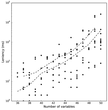
Figure 1. Quantum Annealing Leniency versus Problem Size

This graph suggests an exponential growth in QAL with respect to the problem size. We interpret this as an indication that the difference between the computational time required for our CBQP approach (in conjuction with a scalable UBQP oracle) and the Gurobi Optimizer grows exponentially with the size of the problem.

8. Discussion

In this section we consider the specifics of the D-Wave devices as a physical manifestation of a UBQP oracle. We imagine any implementation of quantum adiabatic computing would have similar limitations, so we expect our algorithms to be beneficial in overcoming them.

Quantum adiabatic devices have not thus far allowed for fully connected systems of quantum bits. Due to this sparsity in the manufactured chips, the use of such quantum computers requires solving a minor-embedding problem, described in the following section, prior to programming the chip according to appropriate couplings and local fields [18].

8.1. Efficient embedding

Given a UBQP instance defined by a matrix $Q$, we define the underlying graph $H$ as follows: for each variable $x_{i}$, we associate a vertex $v_{i}\in V(H)$; and for each nonzero entry $q_{ij}\neq 0$ of $Q$ with $i\neq j$, we let $v_{i}$ and $v_{j}$ be adjacent in $H$. The minor-embedding problem is the problem of finding a function $\phi:V(H)\rightarrow 2^{V(G)}$, where $G$ is the graph defined by the quantum chip (that is, vertices correspond to the quantum bits and edges correspond to the couplings between them), such that

1. for each $x\in V(H)$, the subgraph induced by $\phi(x)$ in $G$ is connected;

2. $\phi(x)$ and $\phi(y)$ are disjoint for all $x\neq y$ in $V(H)$; and,

3. if $x$ and $y$ are adjacent in $H$, there is at least one edge between $\phi(x)$ and $\phi(y)$ in $G$.

Note that for any induced subgraph of $H$, a minor embedding can be found simply by restricting $\phi$ to the vertices of the subgraph. In our CBQP approach, the constraints contribute only to linear terms in the Lagrangian relaxation of the problem, and hence the embedding of a UBQP problem at any node in the branch-and-bound tree can be found from the parent node by restricting the domain of $\phi$. That is, our method requires solving the minor-embedding problem only once, at the root node of the branch-and-bound tree.

8.2. Efficient programming of quantum chips

In every node of the branch-and-bound tree, all Lagrangian relaxations generated have identical quadratic terms and only differ from each other in linear terms. This suggests that if reprogramming the quantum chip can allow for fast updates of previous setups, then the runtime of UBQP oracle queries can also be minimized.

8.3. Error analysis

Quantum bits currently have significant noise. For arbitrary choices of initial and final Hamiltonians, the eigenvalues in the energy spectrum of the evolving Hamiltonian of the system may experience gap closures. Furthermore, the measurement process of the solutions of the quantum adiabatic evolution has a stochastic nature. Each of these obstacles on its own indicates that the solutions read from the quantum system are often very noisy and, even after several repetitions of the process, there is no guarantee of optimality for the corresponding UBQP problem. In order to make our method practical, with a proof of optimality, it is necessary to develop a framework for error analysis for the quantum annealer. Note that for our purposes the solution errors can only propagate to final answers in the branch-and-bound tree if the proposed lower bound $\ell$ obtained at a node is greater than the actual lower bound $\ell-\epsilon$, and the best known upper bound $u$ satisfies $u<\ell$. If this situation occurs, then the proposed method incorrectly prunes the subtree rooted at this node. This motivates the study of a framework of error analysis that can provide a measure of certainty on the optimality of solutions of the UBQP oracle in the above sense.

9. Extension to quadratically constrained problems

It is straightforward to extend the method proposed here to quadratically constrained quadratic programming (QCQP) problems in binary variables. In fact, the Lagrangian relaxations of QCQP problems are also UBQP problems. The minor- embedding problem to be solved at the root node takes the underlying graph $H$ as follows: for each variable $x_{i}$, we associate a vertex $v_{i}\in V(H)$; and for any pair of distinct indices $i\neq j$, we let $(v_{i},v_{j})\in E(H)$ if and only if the term $x_{i}x_{j}$ appears with a nonzero coefficient in the objective function or in any of the quadratic constraints.

Assuming future quantum annealing hardware will allow higher-degree interactions between quantum bits, more-general polynomially constrained binary programming problems could also be solved using a similar approach via Lagrangian duality.

10. Conclusions

Motivated by recent advancements in quantum computing technology, we have provided a method to solve constrained binary programming problems using this technology. Our method is a branch-and-bound algorithm where the lower bounds are computed using Lagrangian duality and queries to an oracle that solves unconstrained binary programming problems.

The conventional branching heuristics for integer programming problems rely on fractional solutions of continuous relaxations of the subproblems at the nodes of the branch-and-bound tree. Our lower-bounding methods are not based on continuous relaxations of the binary variables. In particular, the optimal solutions of the dual problems solved at the nodes of the branch-and-bound tree are not fractional. We proposed several branching strategies that rely on integer solutions and compared their performance both in time and number of nodes visited, and to the conventional branching strategies that rely on fractional solutions.

To compare the performance of our algorithm using quantum hardware against a classical algorithm, we introduced the notion of quantum annealing leniency. This is, roughly speaking, the average time a query to the UBQP oracle would have in order to remain as fast as the benchmark algorithm for solving CBQP problems. In our computational experiments this benchmark algorithm is that of the Gurobi Optimizer.

Finally, although our focus was on quadratic objective functions and linear inequality constraints, in Section 9 we discussed how this method can be generalized to higher-order binary polynomial programming problems.

References

- [1] T. Achterberg, T. Koch and A. Martin (2005), Branching rules revisited, Oper. Res. Lett., Vol. 33(1), pp. 42–54.
- [2] T. Albash, W. Vinci, A. Mishra, P. A. Warburton and D. A. Lidar (2015), Consistency tests of classical and quantum models for a quantum annealer, Phys. Rev. A, Vol. 91, p. 042314.
- [3] B. Alidaee, F. Glover, G. A. Kochenberger and C. Rego (2005), A new modeling and solution approach for the number partitioning problem, J. Appl. Math. Decis. Sci., Vol. 9(2), pp. 113–121.
- [4] B. Alidaee, G. A. Kochenberger and A. Ahmadian (1994), - quadratic programming approach for optimum solutions of two scheduling problems, Internat. J. Systems Sci., Vol. 25(2), pp. 401–408.
- [5] D. Applegate, R. Bixby, V. Chvátal and W. Cook (1995), Finding cuts in the TSP (a preliminary report), Tech. rep., Center for Discrete Mathematics & Theoretical Computer Science.
- [6] A. Assad and W. Xu (1992), The quadratic minimum spanning tree problem, Naval Research Logistics (NRL), Vol. 39(3), pp. 399–417.
- [7] F. Barahona, M. Grötschel, M. Jünger and G. Reinelt (1988), An application of combinatorial optimization to statistical physics and circuit layout design, Oper. Res., Vol. 36(3), pp. 493–513.
- [8] M. Benichou, J. M. Gauthier, P. Girodet, G. Hentges, G. Ribiere and O. Vincent (1971), Experiments in mixed-integer linear programming, Math. Prog., Vol. 1(1), pp. 76–94.
- [9] D. Bertsimas, D. A. Iancu and D. Katz (2013), A new local search algorithm for binary optimization, INFORMS J. Comput., Vol. 25(2), pp. 208–221.
- [10] S. Boixo, V. N. Smelyanskiy, A. Shabani, S. V. Isakov, M. Dykman, V. S. Denchev, M. Amin, A. Smirnov, M. Mohseni and H. Neven (2015), Computational Role of Multiqubit Tunneling in a Quantum Annealer, arXiv:1502.05754.
- [11] I. M. Bomze, M. Budinich, P. M. Pardalos and M. Pelillo (1999), The maximum clique problem, in Handbook of combinatorial optimization, Supplement Vol. A, Kluwer Academic Publishers (Dordrecht), pp. 1–74.
- [12] E. Boros and P. L. Hammer (2002), Pseudo-Boolean optimization, Discrete Appl. Math., Vol. 123(1–3), pp. 155–225.
- [13] E. Boros, P. L. Hammer and G. Tavares (2007), Local search heuristics for quadratic unconstrained binary optimization (QUBO), J. Heuristics, Vol. 13(2), pp. 99–132.
- [14] E. Boros and A. Prékopa (1989), Probabilistic bounds and algorithms for the maximum satisfiability problem, Ann. Oper. Res., Vol. 21(1–4), pp. 109–126.
- [15] J.-M. Bourjolly (1994), A quadratic 0-1 optimization algorithm for the maximum clique and stable set problems, Tech. rep., Univ. of Michigan (Ann Arbor).
- [16] F. Boussemart, F. Hemery, C. Lecoutre and L. Sais (2004), Boosting systematic search by weighting constraints, in ECAI, Vol. 16, p. 146.
- [17] P. I. Bunyk, E. M. Hoskinson, M. W. Johnson, E. Tolkacheva, F. Altomare, A. J. Berkley, R. Harris, J. P. Hilton, T. Lanting, A. J. Przybysz and J. Whittaker (2014), Architectural considerations in the design of a superconducting quantum annealing processor, IEEE Trans. Appl. Supercond., Vol. 24(4), pp. 1–10.
- [18] J. Cai, W. G. Macready and A. Roy (2014), A practical heuristic for finding graph minors, arXiv:1406.2741.
- [19] C. De Simone, M. Diehl, M. Jünger, P. Mutzel, G. Reinelt and G. Rinaldi (1995), Exact ground states of ising spin glasses: New experimental results with a branch-and-cut algorithm, J. Stat. Phys., Vol. 80(1–2), pp. 487–496.
- [20] D.-Z. Du and P. M. Pardalos (Editors) (1999), Handbook of combinatorial optimization. Supplement Vol. A, Kluwer Academic Publishers (Dordrecht).
- [21] E. Farhi, J. Goldstone and S. Gutmann (2000), A Numerical Study of the Performance of a Quantum Adiabatic Evolution Algorithm for Satisfiability, arXiv:quant-ph/0007071.
- [22] E. Farhi, J. Goldstone, S. Gutmann, J. Lapan, A. Lundgren and D. Preda (2001), A quantum adiabatic evolution algorithm applied to random instances of an NP-complete problem, Science, Vol. 292(5516), pp. 472–476.
- [23] C. Floudas and C. Gounaris (2009), A review of recent advances in global optimization, J. Global Optim., Vol. 45(1), pp. 3–38.
- [24] Gurobi Optimization, Inc. (2015), Gurobi Optimizer reference manual.
- [25] R. M. Haralick and G. L. Elliott (1980), Increasing tree search efficiency for constraint satisfaction problems, Artif. Intell., Vol. 14(3), pp. 263–313.
- [26] E. I. Hsu, M. Kitching, F. Bacchus and S. A. McIlraith (2007), Using expectation maximization to find likely assignments for solving CSP’s, in Proceedings of the National Conference on Artificial Intelligence, Vol. 22, American Association for Artificial Intelligence Press (Cambridge MA), p. 224.
- [27] L. D. Iasemidis, P. Pardalos, J. C. Sackellares and D.-S. Shiau (2001), Quadratic binary programming and dynamical system approach to determine the predictability of epileptic seizures, J. Comb. Optim., Vol. 5(1), pp. 9–26.
- [28] M. W. Johnson, M. H. S. Amin, S. Gildert, T. Lanting, F. Hamze, N. Dickson, R. Harris, A. J. Berkley, J. Johansson, P. Bunyk, E. M. Chapple, C. Enderud, J. P. Hilton, K. Karimi, E. Ladizinsky, N. Ladizinsky, T. Oh, I. Perminov, C. Rich, M. C. Thom, E. Tolkacheva, C. J. S. Truncik, S. Uchaikin, J. Wang, B. Wilson and G. Rose (2011), Quantum annealing with manufactured spins, Nature, Vol. 473(7346), pp. 194–198.
- [29] K. Kask, R. Dechter and V. Gogate (2004), Counting-based look-ahead schemes for constraint satisfaction, in Principles and Practice of Constraint Programming–CP 2004, Springer, pp. 317–331.
- [30] H. G. Katzgraber, F. Hamze, Z. Zhu, A. J. Ochoa and H. Munoz-Bauza (2015), Seeking quantum speedup through spin glasses: The good, the bad, and the ugly, Phys. Rev. X, Vol. 5, p. 031026.
- [31] J. Kelly, R. Barends, A. G. Fowler, A. Megrant, E. Jeffrey, T. C. White, D. Sank, J. Y. Mutus, B. Campbell, Y. Chen, Z. Chen, B. Chiaro, A. Dunsworth, I. C. Hoi, C. Neill, P. J. J. O’Malley, C. Quintana, P. Roushan, A. Vainsencher, J. Wenner, A. N. Cleland and J. M. Martinis (2015), State preservation by repetitive error detection in a superconducting quantum circuit, Nature, Vol. 519(7541), pp. 66–69.
- [32] A. D. King and C. C. McGeoch (2014), Algorithm engineering for a quantum annealing platform, arXiv:1410.2628v2.
- [33] G. A. Kochenberger, F. Glover, B. Alidaee and C. Rego (2004), A unified modeling and solution framework for combinatorial optimization problems, OR Spectrum, Vol. 26(2), pp. 237–250.
- [34] E. L. Lawler (1963), The quadratic assignment problem, Management science, Vol. 9(4), pp. 586–599.
- [35] R. Le Bras, A. Zanarini and G. Pesant (2009), Efficient generic search heuristics within the embp framework, in Principles and Practice of Constraint Programming-CP 2009, Springer, pp. 539–553.
- [36] D. Li and X. Sun (2006), Nonlinear integer programming, International Series in Operations Research & Management Science, 84, Springer (New York).
- [37] A. Martin (1998), Integer programs with block structure, Habilitations-Schrift, Technische Universität (Berlin).
- [38] A. Messiah (1962), Quantum mechanics, Vol. II, North-Holland Publishing Co. (Amsterdam).
- [39] M. Oosten, J. H. Rutten and F. C. Spieksma (2001), The clique partitioning problem: facets and patching facets, Networks, Vol. 38(4), pp. 209–226.
- [40] P. M. Pardalos and G. P. Rodgers (1990), Computational aspects of a branch and bound algorithm for quadratic zero-one programming, Computing, Vol. 45(2), pp. 131–144.
- [41] P. M. Pardalos and G. P. Rodgers (1992), A branch and bound algorithm for the maximum clique problem, Comput. Oper. Res., Vol. 19(5), pp. 363–375.
- [42] P. M. Pardalos and J. Xue (1994), The maximum clique problem, J. Global Optim., Vol. 4(3), pp. 301–328.
- [43] G. Pesant, C.-G. Quimper and A. Zanarini (2012), Counting-based search: branching heuristics for constraint satisfaction problems, J. Artif. Intell. Res., Vol. 43, pp. 173–210.
- [44] P. Refalo (2004), Impact-based search strategies for constraint programming, in Principles and Practice of Constraint Programming–CP 2004, Springer, pp. 557–571.
- [45] B. Rostami, F. Malucelli, D. Frey and C. Buchheim (2015), On the quadratic shortest path problem, in Experimental Algorithms, Springer, pp. 379–390.
- [46] P. W. Shor (1994), Algorithms for quantum computation: discrete logarithms and factoring, in 35th Annual Symposium on Foundations of Computer Science, IEEE Comput. Soc. Press (Los Alamitos, CA), pp. 124–134.
- [47] M. Sipser (1996), Introduction to the Theory of Computation, International Thomson Publishing, 1st edn.
- [48] W. van Dam, M. Mosca and U. Vazirani (2001), How powerful is adiabatic quantum computation?, in 42nd IEEE Symposium on Foundations of Computer Science, IEEE Computer Soc. (Los Alamitos, CA), pp. 279–287.
- [49] Y. Wang, Z. Lü, F. Glover and J.-K. Hao (2012), Path relinking for unconstrained binary quadratic programming, European J. Oper. Res., Vol. 223(3), pp. 595–604.
- [50] Z. Zhu, A. J. Ochoa, S. Schnabel, F. Hamze and H. G. Katzgraber (2016), Best-case performance of quantum annealers on native spin-glass benchmarks: How chaos can affect success probabilities, Phys. Rev. A, Vol. 93, p. 012317.