A new model for multi-commodity macroscopic modeling of complex traffic networks

Abstract

We propose a macroscopic modeling framework for a network of roads and multi-commodity traffic. The proposed framework is based on the Lighthill-Whitham-Richards kinematic wave theory; more precisely, on its discretization, the Cell Transmission Model (CTM), adapted for networks and multi-commodity traffic. The resulting model is called the Link-Node CTM (LNCTM).

In the LNCTM, we use the fundamental diagram of an “inverse lambda” shape that allows modeling of the capacity drop and the hysteresis behavior of the traffic state in a link that goes from free flow to congestion and back.

A model of the node with multiple input and multiple output links accepting multi-commodity traffic is a cornerstone of the LNCTM. We present the multi-input-multi-output (MIMO) node model for multi-commodity traffic that supersedes previously developed node models. The analysis and comparison with previous node models are provided.

Sometimes, certain traffic commodities may choose between multiple output links in a node based on the current traffic state of the node’s input and output links. For such situations, we propose a local traffic assignment algorithm that computes how incoming traffic of a certain commodity should be distributed between output links, if this information is not known a priori.

Keywords: macroscopic first order traffic model, first order node model, multi-commodity traffic, dynamic traffic assignment, congestion games, managed lanes

1 Introduction

Traffic simulation models are important tools for traffic engineers and practitioners. As in other disciplines such as climatology, population dynamics, etc., traffic models have helped to deepen our understanding of traffic behavior. They are widely used in transportation planning projects in which capital investments must be justified with simulation-based studies (Caltrans, 2015). Recently, with the increased interest in Integrated Corridor Management (ICM) and Decision Support Systems (DSS), traffic models have found a new role in real-time operations. The requirements for models used in the real-time context, both in terms of execution speed and modeling accuracy, are significantly higher than in the planning context. A model used within an on-line traffic prediction framework, for example, must adapt to incidents, weather changes, special events, as well as to the normal day-to-day variations in demand. It must also be capable of capturing all aspects of the transportation system that are relevant to the operator’s decision making process. These may include arterials as well as freeways, HOV and HOT lanes, ramp meters, variable speed limits, etc. They may also include multiple modes of travel (buses, trains, cars) and their respective emission signatures. Traffic models are also a central component of state estimation (Wright and Horowitz, 2015), in which an entire ensemble of simulations covering a range of possible states must be executed in real time.

The ICM and traffic DSS systems that have been deployed in the U.S. are all driven by microsimulation models. These models simulate the interactions between individual vehicles, and are therefore much more computationally expensive than macroscopic models such as the Cell Transmission Model (Daganzo, 1994, 1995). One of the reasons for this discrepancy is that macroscopic models have lagged behind their commercial microscopic counterparts in their ability to simulate complex configurations such as HOV lanes, arterial/freeway interactions, and multi-commodity flows.

This paper attempts to narrow the gap by introducing some new features for macroscopic models. These features are gathered in a model we call the Link-Node Cell Transmission Model, which, as its name implies, is a generalization of Daganzo’s original CTM. Next we describe each of the new features.

First we introduce a link model that incorporates the notions of capacity drop and hysteresis that have been observed in empirical studies (Srivastava and Gerolimini, 2013). The term “capacity drop” refers to the observation that the maximum flow that can be measured directly downstream of a bottleneck is lower if the bottleneck is active than if it is not (Coifman and Kim, 2010). Hysteresis in traffic dynamics refers to the fact that recovery from congestion usually follows a different path in the flow/density plane than the descent into congestion (Saberi and Mahmassani, 2013). Both of these together can be modeled with a special form of the fundamental diagram commonly referred to as the “inverted lambda” form (Koshi et al., 1983). Of note is that the “inverted lambda” destroys the static functional relationship between flow and density, and therefore requires an extra state, which we will call the “congestion metastate”.

The second contribution of the paper relates to the treatment of network nodes. Node models determine how congestion will travel and distribute from one link to upstream links. For example, the node model determines whether congestion on a freeway will remain on the mainline or spill through the onramps onto the streets. We present a new node model which unifies the existing models of Tampère et al. (2011) and Bliemer (2007). This model uses input link priority parameters and can be applied to multi-commodity traffic. Input link priorities define how output supply should be allocated for incoming flows. In Tampère et al. (2011), input link priorities were assigned implicitly. Our node model admits arbitrary input link priorities.

Third, we propose a relaxation of the first-in-first-out principle (FIFO) that is common to most if not all macroscopic models. The FIFO principle states that all vehicles in a link must travel at the same speed, irrespective of their type or destination. This is not a good approximation in the case of multi-lane traffic, in which each lane is allowed to move at its own speed. Applied to a freeway, it means that congestion backing into the mainline from an offramp will immediately block all lanes. In reality vehicles headed for a congested offramp will tend to queue in the slow lane, while leaving the remaining lanes to continuing traffic. The solution to this problem adopted by authors such as Shiomi et al. (2015) is to assign a state variable to every lane in every link. We propose here a simpler, more computationally efficient scheme in which split ratios are adjusted depending on the downstream availability of space. We allow FIFO to be relaxed across destinations, while preserving FIFO across vehicle types.

The fourth contribution of this article relates to traffic behavior at complex junctions such as access points to managed lanes (e.g., HOV and HOT lanes). Drivers are allowed to choose whether or not to use a managed lane, and they make that choice based on the current observed state of congestion. For example, the incentive to use an HOT lane is greater when the travel time difference between the HOT and the general purpose lanes is large. Thus, a driver’s decision to pay for HOT access will depend on the expected travel times and the price. Split ratios in this situation are not known beforehand – they are endogenous to the model. We develop a split ratio assignment algorithm for this problem in which the split ratios across an HOV or HOT gate are computed by the simulator. This same algorithm may be adapted to other situations in which turning decisions depend on local conditions, as is the case when arterial traffic routes itself around an obstruction.

The paper is organized as follows. Section 2, describes the Link-Node Cell Transmission Model (LNCTM). The main feature of this Section is the “inverse lambda”-shaped fundamental diagram. Section 3 presents our new traffic node model, starting with the analysis of the simpler multiple-input-single-output (MISO) case, then moving to the general multiple-input-multiple-output (MIMO) case. Then, we introduce the relaxed FIFO rule. The proposed node model is used for computing cross-flows into and out of HOV lanes along the freeway. Section 4 describes the split ratio assignment algorithm. Section 5 concludes the paper by summarizing the results. For the convenience of the reader, the notation used in this paper is summarized in the Appendix.

2 Link-Node Cell Transmission Model

The LNCTM models traffic flow in a road network consisting of links ${\cal L}$ and nodes ${\cal N}$, where links represent stretches of roads, and nodes represent junctions that connect links. A node always has at least one input and at least one output link. A link is called ordinary if it has both begin and end nodes. A link with no begin node is called origin, and a link with no end node is called destination. Origins are links through which vehicles enter the system, and destinations are links that let vehicles out.

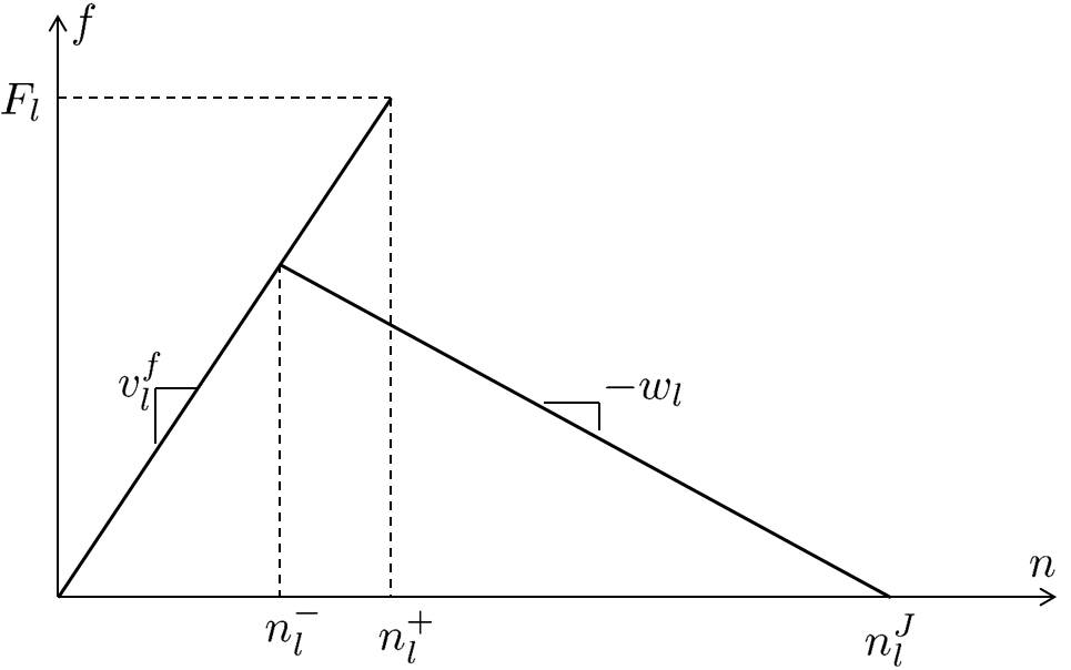
Figure 1: Fundamental diagram.

Each link $l\in{\cal L}$ is characterized by its length and the time dependent fundamental diagram, a flow-density relationship presented in Figure 1. A fundamental diagram may be time-varying and is defined by 4 values: capacity $F_{l}(t)$, free flow speed $v_{l}^{f}(t)$, congestion wave speed $w_{l}(t)$ and the jam density $n^{J}_{l}(t)$. In this paper we assume that densities, flows and speeds are normalized by link lengths and discretization time step; and that free flow speed $v_{l}^{f}(t)$ and congestion wave speed $w_{l}(t)$ satisfy the Courant-Friedrichs-Lewy (CFL) condition (Courant et al., 1928): $0\leq v_{l}^{f}(t),w_{l}(t)\leq 1$. The values $n_{l}^{-}(t)=\frac{w_{l}(t)n_{J}(t)}{v_{l}^{f}(t)+w_{l}(t)}$ and $n_{l}^{+}(t)=\frac{F_{l}(t)}{v_{l}^{f}(t)}$ are called low and high critical density respectively. Unless $n_{l}^{-}(t)=n_{l}^{+}(t)$, when it assumes triangular shape, the fundamental diagram is not a function of density: $n_{l}(t)\in\left(n_{l}^{-}(t),n_{l}^{+}(t)\right]$ admits two possible flow values.

Each node $\nu\in{\cal N}$ with $M$ input and $N$ output links is characterized by time dependent mutual restriction coefficients $\{\eta_{jj^{\prime}}(t)\}^{i}$, input link priorities $\{p_{i}(t)\}$ and partially defined split ratios $\{\beta_{ij}^{c}(t)\}$, where $C$ is the number of vehicle types; $i=1,\dots,M$, $j,j^{\prime}=1,\dots,N$ and $c=1,\dots,C$.

The state of the system at time $t$ is described by the number of vehicles per commodity in each link: $\vec{n}_{l}(t)=\left[n_{l}^{1}(t),\dots,n_{l}^{C}(t)\right]^{T}$, where $n_{l}^{c}(t)$ represents the number of vehicles of type $c$ in link $l$ at time $t$. The state update equation for link $l\in{\cal L}$ is:

$$\vec{n}_{l}(t+1)=\vec{n}_{l}(t)+\left(\vec{f}_{l}^{in}(t)-\vec{f}_{l}^{out}(t)\right),$$ (2.1)

where $\vec{f}_{l}^{in}(t)=\left[f_{l}^{1,in},\dots,f_{l}^{C,in}\right]^{T}$ is the vector of commodity flows coming into link $l$ during this time step, and $\vec{f}_{l}^{out}(t)=\left[f_{l}^{1,out},\dots,f_{l}^{C,out}\right]^{T}$ is the vector of commodity flows leaving link $l$ during this time step.

For ordinary and destination links, $\vec{f}_{l}^{in}(t)$ is obtained from the begin node: given a begin node with $M$ input links,

$$f_{l}^{c,in}(t)=\sum_{i=1}^{M}f_{il}^{c}(t),\;\;\;c=1,\dots,C.$$ (2.2)

For origin links,

$$f_{l}^{c,in}(t)=d_{l}^{c}(t),$$ (2.3)

where $d_{l}^{c}(t)$ denotes commodity demand at time $t$, which is an exogenous input to the model, specified in vehicles per discretization step $\Delta t$.

For ordinary and origin links, $\vec{f}_{l}^{out}(t)$ is obtained from the end node: given an end node with $N$ output links,

$$f_{l}^{c,out}(t)=\sum_{j=1}^{N}f_{lj}^{c}(t),\;\;\;c=1,\dots,C.$$ (2.4)

For destination links,

$$f_{l}^{c,out}(t)=v_{l}^{f}(t)n_{l}^{c}(t)\min\left\{1,\frac{F_{l}(t)}{\sum_{c^{\prime}=1}^{C}v_{l}^{f}(t)n_{l}^{c^{\prime}}(t)}\right\},\;\;\;c=1,\dots,C.$$ (2.5)

The values $f_{il}^{c}(t)$ and $f_{lj}^{c}(t)$ are computed by the node model that is addressed in detail in Section 3.

For each link $l\in{\cal L}$ we will also define a congestion metastate:

$$\theta_{l}(t)=\left\{\begin{array}[]{ll}0&n_{l}(t)\leq n^{-}_{l}(t),\\ 1&n_{l}(t)>n^{+}_{l}(t),\\ \theta_{l}(t-1)&n_{l}^{-}(t)<n_{l}(t)\leq n_{l}^{+}(t),\end{array}\right.$$ (2.6)

where $n_{l}(t)=\sum_{c=1}^{C}n_{l}^{c}(t)$. This metastate helps determining which constraint of the fundamental diagram is activated when we compute the receive function for a link.

Now we can formally describe the LNCTM that runs for $T$ time steps.

1. Initialize:

   $$n_{l}^{c}(0) := n_{l,0}^{c};$$

   $$\theta_{l}(0) := \theta_{l,0};$$

   $$t := 0$$

   for all $l\in{\cal L}$ and $c=1,\dots,C$, where $n_{l,0}^{c}$ and $\theta_{l,0}$ are initial conditions.

2. Apply all the control functions that modify system parameters (fundamental diagrams, input priorities) and/or system state. A control function may represent ramp metering, variable speed limit, managed lane policy, etc. Control functions may be open-loop (if they depend only on time) and closed-loop (if they depend on time and system state). This step is optional.

3. For each link $l\in{\cal L}$ and commodity $c=1,\dots,C$ define the send function:

   $$S_{l}^{c}(t)=\left\{\begin{array}[]{ll}v_{l}^{f}(t)n_{l}^{c}(t)\min\left\{1,\frac{F_{l}(t)}{v_{l}^{f}(t)\sum_{c=1}^{C}n_{l}^{c}(t)}\right\},&l\mbox{ is an ordinary link or a destination},\\ d_{l}^{c}(t)\min\left\{1,\frac{F_{l}(t)}{\sum_{c=1}^{C}d_{l}^{c}(t)}\right\},&l\mbox{ is an origin}.\end{array}\right.$$ (2.7)

4. For each link $l\in{\cal L}$ define the receive function:

   $$R_{l}(t)=\left\{\begin{array}[]{ll}\left(1-\theta_{l}(t)\right)F_{l}(t)+\theta_{l}(t)w_{l}(t)\left(n_{l}^{J}(t)-\sum_{c=1}^{C}n_{l}^{c}(t)\right),&l\mbox{ is an ordinary link or a destination},\\ \infty,&l\mbox{ is an origin}.\end{array}\right.$$ (2.8)

5. For each node $\nu\in{\cal N}$ that has undefined split ratios, given its input link priorities $\{p_{i}(t)\}$, send functions $S_{i}^{c}(t)$ and receive functions $R_{j}(t)$, compute the undefined split ratios $\{\beta_{ij}^{c}(t)\}$ according to the algorithm from Section 4.

6. For each node $\nu\in{\cal N}$, given its mutual restriction coefficients $\{\eta_{jj^{\prime}}^{i}(t)\}$, input link priorities $\{p_{i}(t)\}$ and split ratios $\{\beta_{ij}^{c}(t)\}$, send functions $S_{i}^{c}(t)$ and receive functions $R_{j}(t)$, compute input-output flows $f_{ij}^{c}$ according to the algorithm from Section 3.5.

7. For each link $l\in{\cal L}$, compute $\vec{f}_{l}^{in}(t)$ using expressions (2.2)-(2.3) and $\vec{f}_{l}^{out}(t)$ using expressions (2.4)-(2.5).

8. For each link $l\in{\cal L}$, update the state $\vec{n}_{l}(t+1)$ according to the conservation equation (2.1), and the metastate $\theta_{l}(t+1)$ according to its definition (2.6).

9. If $t=T$, then stop, otherwise set $t:=t+1$ and return to step 2.

Traffic speed for link $l$ is computed as a ratio of total flow leaving this link to the total number of vehicles in this link:

$$v_{l}(t)=\left\{\begin{array}[]{ll}\frac{\sum_{c=1}^{C}f_{l}^{c,out}}{\sum_{c=1}^{C}n_{l}^{c}},&\mbox{ if }\sum_{c=1}^{C}n_{l}^{c}>0,\\ v_{l}^{f}(t),&\mbox{ otherwise}.\end{array}\right.$$ (2.9)

Defined this way, $v_{l}(t)\in[0,v_{l}^{f}(t)]$.

3 Node Model

As mentioned in Section 2, at each timestep of the LNCTM, traffic flows between links are calculated at the node level, such that flows through the node are functions of the state of all links joined at the node (step 5 of the LNCTM algorithm, see Section 2). For nodes with simple link configurations, such as the single-chain case with $M=1,N=1$, these calculations are straightforward, but the present problem requires a node model formulation for computing input-output for general values of $M,N,$ and $C$.

In Tampère et al. (2011), the authors proposed a list of eight requirements for any general node model. With our amendments, this list looks as follows.

1. Applicability to general numbers of input links $M$ and output links $N$. We extend this requirement to include the general number of traffic commodities $C$.

2. Maximization of the total flow coming out of the node. According to Tampère et al. (2011), it means that “each flow should be actively restricted by one of the constraints, otherwise it would increase until it hits some constraint”. When a node model is formulated as a constrained optimization problem, its solution will automatically satisfy this requirement. However, what this requirement really means is that constraints should be stated correctly and not be overly simplified and, thus, overly restrictive for the sake of convenient problem formulation.

3. Non-negativity of all input-output flows.

4. Flow conservation: total flow entering the node must be equal to the total flow exiting. This requirement is automatically satisfied, since we deal directly with input-output flows inside the node.

5. Satisfaction of demand and supply constraints.

6. Satisfaction of the first-in-first-out (FIFO) constraint: if a single destination $j$ for a given $i$ is not able to accept all demand from $i$ to $j$, all flows from $i$ are also constrained.

   We believe that in some situations, the FIFO constraint may be too restrictive. It should not be completely eliminated, however, but must be relaxed through a parametrization. This FIFO relaxation is discribed in Sections 3.4 and 3.5. Parameters that we refer to as mutual restriction coefficients allow configuring each pair of node’s output links to anything between no FIFO at all and fully enforced FIFO.

7. Satisfaction of the invariance principle. If the flow from some input link $i$ is restricted by the available output supply, this input link enters a congested regime. This creates a queue in this input link and causes its demand $S_{i}$ to jump to capacity $F_{i}$ in an infinitesimal time, and therefore, a node model should yield solutions that are invariant to replacing $S_{i}$ with $C_{i}$ when flow from input link $i$ is supply constrained (Lebacque and Khoshyaran, 2005).

   Although the invariance principle is especially important in developing numerical methods for continuous time solutions, whereas our traffic model is discrete in space and time, and its time step $\Delta t$ is not infinitesimal, we retain it in the list of node model requirements and will revisit it in Section 3.3.

8. Satisfaction of the supply constraint interaction rule (SCIR), which is supposed to represent the aggregate driver behavior at congested nodes. Following Gentile et al. (2007), in Tampère et al. (2011) it was proposed to allocate supply for incoming flows proportionally to input link capacities.

   In this paper we propose the concept of input link priorities that can be represented by arbitrary nonnegative values (or functions) as SCIR. Input link priorities will define the allocation of the output supply for incoming flows. It must be noted that the wrong choice of input link priorities may lead to violation of the invariance principle.

We will add the 9th requirement concerning multi-commodity nature of modeled traffic to this list.

1. Supply restriction on a flow from any given input link is imposed on commodity components of this flow proportionally to their presence in this link.

As opposed to the first eight, we do not view requirement 9 as a general principle. Rather, we list it here as a rule that we follow throughout this paper.

Further we will provide the mathematical formulation of the listed requirements and build the node model that satisfies them. This Section is organized as follows. We start by describing the merge problem — the multi-input-multi-output (MISO) node in Section 3.1 to explain the concept of input link priorities. From there we move to the general multi-input-multi-output (MIMO) node in Section 3.2. Then, we discuss the relationship of the proposed node model with the node model of Tampère et al. (2011) and also compare it with the node model presented in Bliemer (2007) in Section 3.3. In Section 3.4 we propose a way of relaxing the FIFO condition and explain it in the case of single-input-multi-output (SIMO) node. Finally, in Section 3.5 we proceed to the general MIMO node with relaxed FIFO condition.

3.1 Multiple-Input-Single-Output (MISO) Node

First, we consider a node with $M$ input links and 1 output link. The number of vehicles of type $c$ that input link $i$ wants to send is $S_{i}^{c}$. The flow entering from input link $i$ has priority $p_{i}\geq 0$. Here $i=1,\dots,M$ and $c=1,\dots,C$. The output link can receive $R$ vehicles.

Casting the computation of input-output flows $f_{i1}^{c}$ as a mathematical programming problem, we arrive at:

$$\max\left(\sum_{i=1}^{M}\sum_{c=1}^{C}f_{i1}^{c}\right),$$ (3.1)

subject to:

$$f_{i1}^{c}\geq 0,\;\;i=1,\dots,M,\;c=1,\dots,C\;\;\mbox{ --- non-negativity constraint};$$ (3.2)

$$f_{i1}^{c}\leq S_{i}^{c},\;\;i=1,\dots,M,\;c=1,\dots,C\;\;\mbox{ --- demand constraint};$$ (3.3)

$$\sum_{i=1}^{M}\sum_{c=1}^{C}f_{i1}^{c}\leq R\;\;\mbox{ --- supply constraint};$$ (3.4)

$$\frac{f_{i1}^{c}}{\sum_{c^{\prime}=1}^{C}f_{i1}^{c^{\prime}}}=\frac{S_{i}^{c}}{\sum_{c^{\prime}=1}^{C}S_{i}^{c^{\prime}}},\;\;i=1,\dots,M,\;c=1,\dots,C,\;\;\mbox{ --- proportionality constraint}$$

$$\mbox{for commodity flows};$$ (3.5)

$$\left.\begin{array}[]{cl}\mbox{(a)}&p_{i^{\prime\prime}}\sum_{c=1}^{C}f_{i^{\prime}1}^{c}=p_{i^{\prime}}\sum_{c=1}^{C}f_{i^{\prime\prime}1}^{c}\;\;\forall i^{\prime},i^{\prime\prime},c,\mbox{ such that }f_{i^{\prime}1}^{c}<S_{i^{\prime}}^{c},\;f_{i^{\prime\prime}1}^{c}<S_{i^{\prime\prime}}^{c},\\ \mbox{(b)}&\mbox{If }\sum_{c=1}^{C}f_{i1}^{c}<\sum_{c=1}^{C}S_{i}^{c},\mbox{ then }\sum_{c=1}^{C}f_{i1}^{c}\geq\frac{p_{i}}{\sum_{i^{\prime}=1}^{M}p_{i^{\prime}}}R.\end{array}\right\}\;\;\mbox{ ---}$$ (3.8)

$$\mbox{priority constraint}.$$ (3.9)

Generally, constraint (3.5) is optional. In this paper, however, we assume that all constraints on input-output flows are imposed on commodity flows proportionally to commodity contributions to total demand. This constraint can be interpreted as a FIFO rule for multi-commodity traffic within a given link; not to be confused with the FIFO rule for multiple output links.

Let us discuss priority constraint (3.9) in more detail. It should be interpreted as follows. Input links $i=1,\dots,M$, fall into two categories: (1) those whose flow is restricted by the allocated supply of the output link; and (2) those whose demand is satisfied by the supply allocated for them in the output link. Priorities define how supply in the output link is allocated for input flows. Condition (3.9)(a) says that flows from input links of category 1 are allocated proportionally to their priorities. Condition (3.9)(b) ensures that input flows of category 2 do not take up more output supply than was allocated for them in cases where category 1 is non-empty. The inequality in Condition (3.9)(b) becomes an equality when category 2 is empty.

There is a special case, when some input link priorities are equal to $0$. If there exists input link $\hat{\imath}$, such that $p_{\hat{\imath}}=0$, while $f_{\hat{\imath}1}>0$, then, due to condition (3.9)(a), all input links with non-zero priorities are in category 2. Thus, if category 1 contains only input links with zero priorities, one should evaluate condition (3.9)(a) with arbitrary positive, but equal, priorities: $p_{i^{\prime}}=p_{i^{\prime\prime}}>0$.

If the priorities $p_{i}$ are proportional to send functions $\sum_{c=1}^{C}S_{i}$, $i=1,\dots,M$, then condition (3.9) can be written as an equality constraint:

$$\frac{\sum_{c=1}^{C}f_{11}^{c}}{\sum_{c=1}^{C}S_{1}^{c}}=\dots=\frac{\sum_{c=1}^{C}f_{i1}^{c}}{\sum_{c=1}^{C}S_{i}^{c}}=\dots=\frac{\sum_{c=1}^{C}f_{M1}^{c}}{\sum_{c=1}^{C}S_{M}^{c}},$$ (3.10)

and the optimization problem (3.1)-(3.9) turns into a linear program (LP).

For arbitrary priorities with $M=2$, condition (3.9) becomes:

$$\sum_{c=1}^{C}f_{11}^{c}\leq\max\left\{\frac{p_{1}}{p_{1}+p_{2}}R,\;R-\sum_{c=1}^{C}S_{2}^{c}\right\};$$ (3.11)

$$\sum_{c=1}^{C}f_{21}^{c}\leq\max\left\{\frac{p_{2}}{p_{1}+p_{2}}R,\;R-\sum_{c=1}^{C}S_{1}^{c}\right\}.$$ (3.12)

To give a hint how more complicated constraint (3.9) becomes as $M$ increases, let us write it out for $M=3$:

$$\sum_{c=1}^{C}f_{11}^{c}\leq\max\left\{\frac{p_{1}}{\sum_{i=1}^{3}p_{i}}R,\frac{p_{1}}{p_{1}+p_{2}}\left(R-\sum_{c=1}^{C}S_{3}^{c}\right),\frac{p_{1}}{p_{1}+p_{3}}\left(R-\sum_{c=1}^{C}S_{2}^{c}\right),R-\sum_{i=2,3}\sum_{c=1}^{C}S_{i}^{c}\right\};\\$$ (3.13)

$$\sum_{c=1}^{C}f_{21}^{c}\leq\max\left\{\frac{p_{2}}{\sum_{i=1}^{3}p_{i}}R,\frac{p_{2}}{p_{1}+p_{2}}\left(R-\sum_{c=1}^{C}S_{3}^{c}\right),\frac{p_{2}}{p_{2}+p_{3}}\left(R-\sum_{c=1}^{C}S_{1}^{c}\right),R-\sum_{i=1,3}\sum_{c=1}^{C}S_{i}^{c}\right\};$$ (3.14)

$$\sum_{c=1}^{C}f_{31}^{c}\leq\max\left\{\frac{p_{3}}{\sum_{i=1}^{3}p_{i}}R,\frac{p_{3}}{p_{1}+p_{3}}\left(R-\sum_{c=1}^{C}S_{2}^{c}\right),\frac{p_{3}}{p_{2}+p_{3}}\left(R-\sum_{c=1}^{C}S_{1}^{c}\right),R-\sum_{i=1,2}\sum_{c=1}^{C}S_{i}^{c}\right\}.$$ (3.15)

As we can see, right hand sides of inequalities (3.13)-(3.15) contain known quantities, and so for arbitrary priorities, problem (3.1)-(3.9) is also an LP. For general $M$, however, building constraint (3.9) requires a somewhat involved algorithm. Instead, we present the algorithm for computing input-output flows $f_{i1}^{c}$ that solves the maximization problem (3.1)-(3.9).

1. Initialize:

   $$\tilde{R}(0) := R;$$

   $$U(0) := \left\{1,\dots,M\right\};$$

   $$k := 0.$$

   $U(k)$ is the set of unprocessed input links: input links whose input-output flows have not been assigned yet.

2. Check that at least one of the unprocessed input links has nonzero priority, otherwise, assign equal positive priorities to all the unprocessed input links:

   $$\tilde{p}_{i}(k)=\left\{\begin{array}[]{ll}p_{i},&\mbox{ if there exists }i^{\prime}\in U(k):\;p_{i^{\prime}}>0,\\ \frac{1}{|U(k)|},&\mbox{ otherwise},\end{array}\right.$$

   where $|U(k)|$ denotes the number of elements in set $U(k)$.

3. Define the set of input links that want to send fewer vehicles than their allocated supply and whose flows are still undetermined:

   $$\tilde{U}(k)=\left\{i\in U(k):\;\sum_{c=1}^{C}S_{i}^{c}\leq\tilde{p}_{i}(k)\frac{\tilde{R}(k)}{\sum_{i^{\prime}\in U(k)}\tilde{p}_{i^{\prime}}(k)}\right\}.$$

   • If $\tilde{U}(k)\neq\emptyset$, assign:

     $$f_{i1}^{c} = S_{i}^{c},\;\;\;i\in\tilde{U}(k);$$

     $$\tilde{R}(k+1) = \tilde{R}(k)-\sum_{i\in\tilde{U}}\sum_{c=1}^{C}f_{i1}^{c};$$

     $$U(k+1) = U(k)\setminus\tilde{U}(k).$$

   • Else, assign:

     $$f_{i1}^{c} = S_{i}^{c}\frac{\tilde{p}_{i}(k)}{\sum_{i^{\prime}\in U(k)}\tilde{p}_{i^{\prime}}(k)}\frac{\tilde{R}(k)}{\sum_{c=1}^{C}S_{i}^{c}},\;\;\;i\in U(k);$$

     $$U(k+1) = \emptyset.$$

4. If $U(k+1)=\emptyset$, then stop.

5. Set $k:=k+1$, and return to step 2.

This algorithm finishes after no more than $M$ iterations, and in the special case of $M=2$ it reduces to

$$f_{11}^{c} = \min\left\{S_{1}^{c},\;\;S_{1}^{c}\frac{\max\left\{\frac{p_{1}}{p_{1}+p_{2}}R,\;\;R-\sum_{c^{\prime}=1}^{C}S_{2}^{c^{\prime}}\right\}}{\sum_{c^{\prime}=1}^{C}S_{1}^{c^{\prime}}}\right\};$$ (3.16)

$$f_{21}^{c} = \min\left\{S_{2}^{c},\;\;S_{2}^{c}\frac{\max\left\{\frac{p_{2}}{p_{1}+p_{2}}R,\;\;R-\sum_{c^{\prime}=1}^{C}S_{1}^{c^{\prime}}\right\}}{\sum_{c^{\prime}=1}^{C}S_{2}^{c^{\prime}}}\right\}.$$ (3.17)

The following theorem can be trivially proved, and we leave the proof to the reader. Further, in Section 3.5, it will become clear that this theorem is a special case of a more general statement.

Theorem 3.1.

The input-output flow computation algorithm constructs the unique solution of the maximization problem (3.1)-(3.9).

Example. Suppose we have three inputs and one output, with parameters:

$C=1$	$R=1000$
$S_{1}=400$	$p_{1}=\nicefrac{{1}}{{3}}$
$S_{2}=500$	$p_{2}=\nicefrac{{2}}{{3}}$
$S_{3}=200$	$p_{3}=0$

Our solution algorithm for finding the resulting flows proceeds as follows:

$$\underline{k=0:}$$

$$1.\qquad U(0)=\{1,2,3\};\quad\tilde{R}(0)=1000;$$

$$2.\qquad\tilde{p}_{1}(0)=\nicefrac{{1}}{{3}},\;\tilde{p}_{2}(0)=\nicefrac{{2}}{{3}},\;\tilde{p}_{3}(0)=0$$

$$3.\qquad\tilde{U}(0)=\{2\};\quad\boldsymbol{f_{2}=500};\quad\tilde{R}(1)=500;\quad U(1)=\{1,3\}$$

$$\underline{k=1:}$$

$$2.\qquad\tilde{p}_{1}(1)=\nicefrac{{1}}{{3}},\;\tilde{p}_{3}(1)=0$$

$$3.\qquad\tilde{U}(1)=\{1\};\quad\boldsymbol{f_{1}=400};\quad\tilde{R}(2)=100;\quad U(2)=\{3\}$$

$$\underline{k=2:}$$

$$2.\qquad\tilde{p}_{3}(2)=1$$

$$3.\qquad\tilde{U}(2)=\emptyset;\quad\boldsymbol{f_{3}=100};\quad U(3)=\emptyset$$

3.2 Multiple-Input-Multiple-Output (MIMO) Node

Now we consider the general case: a node with $M$ input, $N$ output links and $C$ traffic commodities. Given are input demands $S_{i}^{c}$ and split ratios $\beta_{ij}^{c}$ specified per commodity, input priorities $p_{i}\geq 0$, and output supply $R_{j}$.

Define oriented demand:

$$S_{ij}^{c}=\beta_{ij}^{c}S_{i}^{c},$$ (3.18)

and oriented priorities:

$$p_{ij}=p_{i}\frac{\sum_{c=1}^{C}S_{ij}^{c}}{\sum_{c=1}^{C}S_{i}^{c}},$$ (3.19)

where $i=1,\dots,M$, $j=1,\dots,N$ and $c=1,\dots,C$.

As before, we start by casting the allocation of input-output flows $f_{ij}^{c}$ as a constrained optimization problem:

$$\max\left(\sum_{i=1}^{M}\sum_{j=1}^{N}\sum_{c=1}^{C}f_{ij}^{c}\right),$$ (3.20)

subject to:

$$f_{ij}^{c}\geq 0,\;\;i=1,\dots,M,\;j=1,\dots,N,\;c=1,\dots,C\;\mbox{ --- non-negativity constraint};$$ (3.21)

$$f_{ij}^{c}\leq S_{ij}^{c},\;\;i=1,\dots,M,\;j=1,\dots,N,\;c=1,\dots,C\;\mbox{ --- demand constraint};$$ (3.22)

$$\sum_{i=1}^{M}\sum_{c=1}^{C}f_{ij}^{c}\leq R_{j},\;\;j=1,\dots,N\;\mbox{ --- supply constraint};$$ (3.23)

$$\frac{f_{ij}^{c}}{\sum_{c^{\prime}=1}^{C}f_{ij}^{c^{\prime}}}=\frac{S_{ij}^{c}}{\sum_{c^{\prime}=1}^{C}S_{ij}^{c^{\prime}}},\;\;i=1,\dots,M,\;j=1,\dots,N,c=1,\dots,C\;\;\mbox{ --- proportionality}$$

$$\mbox{constraint for commodity flows};$$ (3.24)

$$\frac{\sum_{c=1}^{C}f_{ij}^{c}}{\sum_{j=1}^{N}\sum_{c=1}^{C}f_{ij}^{c}}=\frac{\sum_{c=1}^{C}S_{ij}^{c}}{\sum_{j=1}^{N}\sum_{c=1}^{C}S_{ij}^{c}},\;\;i=1,\dots,M\;\;\mbox{ --- FIFO constraint};$$ (3.25)

$$\left.\begin{array}[]{cl}\mbox{(a)}&\mbox{For each input link $i$, such that }\\ &\sum_{j=1}^{N}\sum_{c=1}^{C}f_{ij}^{c}<\sum_{c=1}^{C}S_{i}^{c},\\ &\mbox{there exists an output link $j^{\ast}$, such that }\\ &p_{i^{\prime}j^{\ast}}\sum_{c=1}^{C}f_{ij^{\ast}}^{c}\geq p_{ij^{\ast}}\sum_{c=1}^{C}f_{i^{\prime}j^{\ast}}^{c}\forall i^{\prime}\neq i,\\ &\mbox{and it is said that output $j^{\ast}$ restricts input flow $i$};\\ \mbox{(b)}&\mbox{For each input link $i$ whose flow is restricted by some output $j$,}\\ &\sum_{c=1}^{C}f_{ij}^{c}\geq\frac{p_{ij}}{\sum_{i^{\prime}=1}^{M}p_{i^{\prime}j}}R_{j}.\end{array}\right\}\mbox{ --- priority constraint}.$$ (3.26)

Here, the objective function (3.20) and constraints (3.21)-(3.24) are straight forward extensions of the objective function (3.20) and constraints (3.2)-(3.5). The FIFO constraint (3.25) ensures that, for a given input link $i$, if any one of the output links is unable to accommodate its allocation of flow, all outflow from $i$ is restricted proportionally (Daganzo, 1994, 1995).

Let us focus the attention on the priority constraint (3.26). Condition (3.26)(a) says that if the flow from a given input link $i$ is reduced by the output supply, there must be the most restrictive output link, which is denoted $j^{\ast}$. If the output $j^{\ast}$ restricts flows from input links $i^{\prime}$ and $i^{\prime\prime}$, then, according to condition (3.26)(a),

$$p_{i^{\prime\prime}j^{\ast}}\sum_{c=1}^{C}f_{i^{\prime}j^{\ast}}^{c}=p_{i^{\prime}j^{\ast}}\sum_{c=1}^{C}f_{i^{\prime\prime}j^{\ast}}^{c}.$$

For each output link $j$, $j=1,\dots,N$, flows $\sum_{c=1}^{C}f_{ij}^{c}$ fall into two categories: (1) restricted by this output link; and (2) not restricted by this output link. Condition (3.26)(a) states that input-output flows of category 1 are allocated proportionally to their priorities. For every output link $j$, $j=1,\dots,N$, condition (3.26)(b) ensures that input-output flows of category 2 do not take up more output supply than was allocated for them when category 1 is non-empty.

Recalling the MISO case, we can see that for $N=1$, formulation (3.20)-(3.26) translates to formulation (3.1)-(3.9).

Remark. It must be noted here that when priorities $p_{i}$ are proportional to send functions $\sum_{c=1}^{C}S_{i}$, $i=1,\dots,M$, and $M>1$, the condition (3.26) cannot be written simply as an extension of (3.10) for any output link $j$, $j=1,\dots,N$, as was done by Bliemer in (2007). He used the constraint

$$\frac{\sum_{c=1}^{C}f_{1j}^{c}}{\sum_{c=1}^{C}S_{1j}^{c}}=\dots=\frac{\sum_{c=1}^{C}f_{ij}^{c}}{\sum_{c=1}^{C}S_{ij}^{c}}=\dots=\frac{\sum_{c=1}^{C}f_{Mj}^{c}}{\sum_{c=1}^{C}S_{Mj}^{c}},\;\;j=1,\dots,N,$$ (3.27)

in the place of (3.26), which reduces the optimization problem (3.20)-(3.26) to an LP. While suitable for $N=1$, expression (3.27) is not an adequate representation of the constraint (3.26) for $N>1$, because it leads to the underutilization of the available supply, as will be shown in Section 3.3.

Next, we present the algorithm for constructing the unique solution of the optimization problem (3.20)-(3.26).

1. Initialize:

   $$\tilde{R}_{j}(0) := R_{j};$$

   $$U_{j}(0) := \left\{i\in\{1,\dots,M\}:\;\sum_{c=1}^{C}S_{ij}^{c}>0\right\};$$

   $$k := 0;$$

   $$i=1,\dots,M,\;\;\;j=1,\dots,N,\;\;\;c=1,\dots,C.$$

   $U_{j}(k)$ is the set of input links contributing traffic to output link $j$, whose input-output flows are still unassigned.

2. Define the set of output links that still need processing:

   $$V(k)=\left\{j\in\{1,\dots,N\}:\;U_{j}(k)\neq\emptyset\right\}.$$

   If $V(k)=\emptyset$, stop.

3. Check that at least one of the unprocessed input links has nonzero priority, otherwise, assign equal positive priorities to all the unprocessed input links:

   $$\tilde{p}_{i}(k)=\left\{\begin{array}[]{ll}p_{i},&\mbox{ if there exists }i^{\prime}\in\bigcup_{j\in V(k)}U_{j}(k):\;p_{i^{\prime}}>0,\\ \frac{1}{\left|\bigcup_{j\in V(k)}U_{j}(k)\right|},&\mbox{ otherwise},\end{array}\right.$$ (3.28)

   where $\left|\bigcup_{j\in V(k)}U_{j}(k)\right|$ denotes the number of elements in the union $\bigcup_{j\in V(k)}U_{j}(k)$; and for each output link $j\in V(k)$ and input link $i\in U_{j}(k)$ compute oriented priority:

   $$\tilde{p}_{ij}(k)=\tilde{p}_{i}(k)\frac{\sum_{c=1}^{C}S_{ij}^{c}}{\sum_{c=1}^{C}S_{i}^{c}}.$$ (3.29)

4. For each $j\in V(k)$, compute factors:

   $$a_{j}(k)=\frac{\tilde{R}_{j}(k)}{\sum_{i\in U_{j}(k)}\tilde{p}_{ij}(k)},$$ (3.30)

   and find the smallest of these factors:

   $$a_{j^{\ast}}(k)=\min_{j\in V(k)}a_{j}(k).$$ (3.31)

   The link $j^{\ast}$ has the most restricted supply of all output links.

5. Define the set of input links, whose demand does not exceed the allocated supply:

   $$\tilde{U}(k)=\left\{i\in U_{j^{\ast}}(k):\;\sum_{c=1}^{C}S_{i}^{c}\leq\tilde{p}_{i}(k)a_{j^{\ast}}(k)\right\}.$$

   • If $\tilde{U}(k)\neq\emptyset$, then for all output links $j\in V(k)$ assign:

     $$f_{ij}^{c} = S_{ij}^{c},\;\;\;i\in\tilde{U}(k),\;\;c=1,\dots,C;$$

     $$\tilde{R}_{j}(k+1) = \tilde{R}_{j}(k)-\sum_{i\in\tilde{U}(k)}\sum_{c=1}^{C}f_{ij}^{c};$$

     $$U_{j}(k+1) = U_{j}(k)\setminus\tilde{U}(k).$$

   • Else, for all input links $i\in U_{j^{\ast}}(k)$ and output links $j\in V(k)$ assign:

     $$f_{ij}^{c} = S_{ij}^{c}\frac{\tilde{p}_{ij}(k)a_{j^{\ast}}(k)}{\sum_{c^{\prime}=1}^{C}S_{ij}^{c^{\prime}}},\;\;\;i\in U_{j}(k)\cap U_{j^{\ast}}(k);$$ (3.32)

     $$\tilde{R}_{j}(k+1) = \tilde{R}_{j}(k)-\sum_{i\in U_{j^{\ast}}(k)}\sum_{c=1}^{C}f_{ij}^{c};$$

     $$U_{j}(k+1) = U_{j}(k)\setminus U_{j^{\ast}}(k),$$

     where, obviously, $U_{j^{\ast}}(k+1)=\emptyset$.

6. Set $k:=k+1$, and return to step 2.

This algorithm takes no more than $M$ iterations to complete.

The following lemma states that in the case of $N=1$, the MIMO algorithm produces exactly the same result as the MISO algorithm described in Section 3.1.

Lemma 3.1.

The MISO algorithm is a special case of the MIMO algorithm with $N=1$.

Proof.

The proof follows from the fact that for $N=1$, formulae (3.30)-(3.31) result in $a_{j^{\ast}}(k)=a_{1}(k)=\frac{\tilde{R}_{1}(k)}{\sum_{i\in U_{1}(k)}\tilde{p}_{i}(k)}$ and $j^{\ast}=1$. ∎

The following theorem is the analog of Theorem 3.1. As in the MISO case, we leave the proof out, since a more general statement will be proved in Section 3.5.

Theorem 3.2.

The input-output flow computation algorithm constructs the unique solution of the maximization problem (3.20)-(3.26).

3.3 Relationship with Tampére Et Al. and Bliemer Node Models

It can be shown that the node model described here is a slight generalization of the Tampére et al. unsignalized node model developed in Tampère et al. (2011), In particular, for a specific choice of priorities, $p_{i}$, the equations of section 3.2 become exactly the equations of this model.

Theorem 3.3.

By setting the priorities for the MIMO model equal to the link capacity, $F$,

$$p_{i}=F_{i},$$

with $F_{i}$ the capacity of link $i$, we obtain the Tampére et al. node model.

Proof.

The Tampére et al. model does not deal with multiple commodities, so first, let $C=1$ and drop the commodity index $c$. Then, our oriented priorities (3.29) become:

$$\tilde{p}_{ij}=F_{i}\frac{S_{ij}}{S_{i}}.$$

Again for simplicity, assume that we do not have any input links whose demands can be wholly met. Then, the smallest $a_{j}(k)$ factor is

$$a_{j^{\ast}}=\min_{j\in V(k)}\frac{\tilde{R}_{j}}{\sum_{i\in U_{j}(k)}F_{i}\frac{S_{ij}}{S_{i}}}$$

and the resulting flows are

$$f_{ij}=S_{ij}\frac{\tilde{p}_{ij}(k)a_{j^{\ast}}(k)}{S_{ij}}=\tilde{p}_{ij}(k)a_{j^{\ast}}(k)=F_{i}\frac{S_{ij}}{S_{i}}\frac{\tilde{R}_{j^{\ast}}}{\sum_{i\in U_{j^{\ast}}}F_{i}\frac{S_{ij^{\ast}}}{S_{i}}}$$ (3.33)

comparing the above development to equations (19), (24), (26), and (28) in Tampère et al. (2011), we have recovered exactly the Tampére et al. node model. ∎

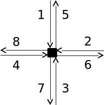
Figure 2: A 4-by-4 example intersection.

Example. This specific example is taken from Tampére et al. (2011), to illustrate both the procedure of our MIMO node algorithm and the equivalence of our node model to the Tampére et al. model proved above.

Consider the 4-by-4 intersection shown in Figure 2. Suppose that our relevant parameters are:

$C=1$
$S_{1}=500$	$S_{2}=2000$	$S_{3}=800$	$S_{4}=1700$
$p_{1}=F_{1}=1000$	$p_{2}=F_{2}=2000$	$p_{3}=F_{3}=1000$	$p_{4}=F_{4}=2000$
$R_{5}=1000$	$R_{6}=2000$	$R_{7}=1000$	$R_{8}=2000$
$\beta_{15}=0$	$\beta_{16}=0.1$	$\beta_{17}=0.3$	$\beta_{18}=0.6$
$\beta_{25}=0.05$	$\beta_{26}=0$	$\beta_{27}=0.15$	$\beta_{28}=0.8$
$\beta_{35}=0.125$	$\beta_{36}=0.125$	$\beta_{37}=0$	$\beta_{38}=0.75$
$\beta_{45}=\nicefrac{{1}}{{17}}$	$\beta_{46}=\nicefrac{{8}}{{17}}$	$\beta_{47}=\nicefrac{{8}}{{17}}$	$\beta_{48}=0$

Our solution algorithm proceeds as follows:

First, compute oriented demands:

$S_{15}=0$	$S_{16}=50$	$S_{17}=150$	$S_{18}=300$
$S_{25}=100$	$S_{26}=0$	$S_{27}=300$	$S_{28}=1600$
$S_{35}=100$	$S_{36}=100$	$S_{37}=0$	$S_{38}=600$
$S_{45}=100$	$S_{46}=800$	$S_{47}=800$	$S_{48}=0.$

$k=0:$

1. $U_{5}(0)=\{2,3,4\};\quad U_{6}(0)=\{1,3,4\};\quad U_{7}(0)=\{1,2,4\};\quad U_{8}(0)=\{1,2,3\}$

2. $V(0)=\{5,6,7,8\}$

3. No adjustments to the $\tilde{p}_{i}$ are made. The oriented priorities are:
   $\tilde{p}_{15}=0$ $\tilde{p}_{16}=100$ $\tilde{p}_{17}=300$ $\tilde{p}_{18}=600$ $\tilde{p}_{25}=100$ $\tilde{p}_{26}=0$ $\tilde{p}_{27}=300$ $\tilde{p}_{28}=1600$ $\tilde{p}_{35}=125$ $\tilde{p}_{36}=125$ $\tilde{p}_{37}=0$ $\tilde{p}_{38}=750$ $\tilde{p}_{45}=118$ $\tilde{p}_{46}=941$ $\tilde{p}_{47}=941$ $\tilde{p}_{48}=0$

4. $a_{5}(0)=2.92;\quad a_{6}(0)=1.72;\quad a_{7}(0)=0.649;\quad a_{8}(0)=0.678$
   $a_{j^{\ast}}(0)=a_{7}(0)=0.649$

5. $\tilde{U}(0)=\{1\},\text{ as }S_{1}=500\leq\tilde{p}_{1}(0)a_{7}(0)=1000\times 0.649$

   • $\boldsymbol{f_{16}=S_{16}=50;}\quad\boldsymbol{f_{17}=S_{17}=150;}\quad\boldsymbol{f_{18}=S_{18}=300;}$

   • $\tilde{R}_{6}(1)=2000-50=1950;\quad\tilde{R}_{7}(1)=1000-150=850;\quad\tilde{R}_{8}(1)=2000-300=1700$

   • $U_{5}(1)=\{2,3,4\};\quad U_{6}(1)=\{3,4\};\quad U_{7}(1)=\{2,4\};\quad U_{8}(1)=\{2,3\}$

$k=1:$

1. $V(1)=\{5,6,7,8\}$

2. No changes are made to priorities or oriented priorities.

3. $a_{5}(1)=2.92;\quad a_{6}(1)=1.83;\quad a_{7}(1)=0.685;\quad a_{8}(0)=0.723$
   $a_{j^{\ast}}(1)=a_{7}(1)=0.685$

4. $\tilde{U}(1)=\emptyset,$ as $S_{2}=2000\nleq\tilde{p}_{2}(1)a_{7}(1)=1370,$ and $S_{4}=1700\nleq\tilde{p}_{4}(1)a_{7}(1)=1370,$

   • $\boldsymbol{f_{25}=\tilde{p}_{25}(1)a_{7}(1)=68.5}$

   • $\boldsymbol{f_{27}=\tilde{p}_{27}(1)a_{7}(1)=205.5}$

   • $\boldsymbol{f_{28}=\tilde{p}_{28}(1)a_{7}(1)=1096}$

   • $\boldsymbol{f_{45}=\tilde{p}_{45}(1)a_{7}(1)=80.6}$

   • $\boldsymbol{f_{46}=\tilde{p}_{46}(1)a_{7}(1)=644.5}$

   • $\boldsymbol{f_{47}=\tilde{p}_{47}(1)a_{7}(1)=644.5}$

   • $\tilde{R}_{5}(2)=1000-68.5-80.6=850.9;\quad\tilde{R}_{6}(2)=1950-644=1305.5;$
     $\tilde{R}_{7}(2)=850-644.5-204.5=0;\quad\tilde{R}_{8}(2)=1700-1096=604$

   • $U_{5}(2)=\{3\};\quad U_{6}(2)=\{3\};\quad U_{7}(2)=\emptyset;\quad U_{8}(2)=\{3\}$

$k=2:$

1. $V(2)=\{5,6,8\}$

2. No changes are made to priorities or oriented priorities.

3. $a_{5}(2)=6.81;\quad a_{6}(2)=10.45;\quad a_{8}(2)=0.805$
   $a_{j^{\ast}}(2)=a_{8}(2)=0.805$

4. $\tilde{U}(2)=\{3\},$ as $S_{3}=800\leq\tilde{p}_{3}(2)a_{8}(2)=805$

   • $\boldsymbol{f_{35}=S_{35}=100;}\quad\boldsymbol{f_{36}=S_{36}=100;}\quad\boldsymbol{f_{38}=S_{38}=600;}$

   • $U_{j}(3)=\emptyset\quad\forall j$

$k=3:$

1. $V(3)=\emptyset$, so the algorithm terminates. All flows have been found.

As discussed in Section 3.2, for $N>1$ the demand-proportional priority node model of Bliemer (2007) cannot be written as a special case of this node model, and that replacing the priority constraint (3.26) with a constraint of the form (3.27) leads to underused supply. Let us consider a simple example:

Example. Suppose we have a 2-by-2 intersection, with parameters

$C=1$		$p_{1}=0.5$	$p_{2}=0.5$
$S_{1}=1000$	$S_{2}=1000$	$R_{1}=600$	$R_{2}=1000$
$\beta_{11}=\nicefrac{{9}}{{10}}$	$\beta_{12}=\nicefrac{{1}}{{10}}$
$\beta_{21}=0$	$\beta_{22}=1$

It should be clear that our algorithm will solve this problem in two iterations. In the first iteration, we will have

$$a_{1}(0) =\nicefrac{{600}}{{900}}=\nicefrac{{2}}{{3}}=a_{j^{\ast}}(0)$$

$$a_{2}(0) =\nicefrac{{1000}}{{1100}}=\nicefrac{{10}}{{11}}$$

and, as $U_{j^{\ast}}(0)=U_{1}(0)=\{1\}$, the flows found will be

$$f_{11} =600$$

$$f_{12} =\nicefrac{{2}}{{3}}\times 100\approx 67.$$

In the second iteration, link $i=2$ will fill up all remaining space in link $j=2$:

$$f_{21} =0$$

$$f_{22} =R_{2}-f_{12}\approx 933,$$

and the total flow passing through the node is

$$f_{11}+f_{12}+f_{21}+f_{22}=1600.$$

On the other hand, in the Bliemer model we first encounter the supply restriction $R_{1}$ that, together with the FIFO constraint (3.25), reduces the flow from input link 1 by the factor $\nicefrac{{2}}{{3}}$, and we get

$$f_{11} =600$$

$$f_{12} =\nicefrac{{2}}{{3}}\times 100\approx 67,$$

just as in our calculation above. There is no flow from input link 2 to output link 1: $f_{21}=0$. Next, condition (3.27) implies that

$$\frac{f_{11}}{S_{11}}=\frac{f_{12}+f_{22}}{S_{12}+S_{22}}=\frac{600}{900},$$

which yields:

$$f_{22}=\frac{2}{3}(S_{12}+S_{22})-f_{21}\approx 667,$$

and so, the total flow through the node is

$$f_{11}+f_{12}+f_{21}+f_{22}=1334.$$

As we see, the Bliemer model violates requirement 2 from the list in the beginning of Section 3: it does not maximize the total flow through the node. Failure to maximize the flow happened in the LP setting of Bliemer (2007) due to the incorrect constraint (3.27) that was imposed in pursuit of an easy formulation of the optimization problem.

It was shown in Tampère et al. (2011) that the Bliemer model also violates the invariance principle — requirement 7 from the list. The violation of the invariance principle happened because supply allocation was governed by the input demand. The input link started to congest, and the demand jumped in infinitely small time, which immediately triggered change in the supply allocation of the output link, ultimately resulting in discontinuous flow. In a discrete time system, such as LNCTM, these considerations may be simply ignored. However, since our proposed node model is generic and can be used outside of the LNCTM, we should note that to avoid violating the invariance principle, input link priorities must not depend on traffic state.

3.4 Single-Input-Multiple-Output (SIMO) Node with Relaxed FIFO Condition

Sometimes the FIFO rule may be too restrictive. An example of such situation is a junction, where a 1-lane off-ramp diverges from a 5-lane freeway, especially, if this off-ramp is relatively short and terminates with a signal. Jammed off-ramp blocks the flow on the whole freeway, which is not realistic. A more realistic behavior would be for this jammed off-ramp to only partially restrict the mainline flow. For instance, one could say that this off-ramp restricts only 40% of the mainline traffic. On the other hand, if the mainline happens to be jammed, we want 100% of the off-ramp traffic to be restricted. Thus, in a given diverge junction FIFO restrictions on outgoing flows are not symmetric. The model of a diverge node with a partial FIFO restriction is described next.

Consider a node with a single input and $N$ output links. Given are the input demand per commodity, $S^{c}$, $c=1,\dots,C$, the output supply $R_{j}$, split ratios $\beta_{1j}^{c}$, $j=1,\dots,N$, and the mutual restriction matrix $\{\eta_{jj^{\prime}}\}\in\mathbb{R}^{N\times N}$, $\eta_{jj^{\prime}}\in[0,1]$, $\eta_{jj}=1$. Element $\eta_{jj^{\prime}}$ of the mutual restriction matrix specifies the portion of the flow in the output link $j^{\prime}$ affected by the restriction of the output link $j$. In the example above, where the mainline output link is identified as 1 and the off-ramp as 2, this matrix assumes the form $\left[\begin{array}[]{cc}1&1\\ 0.4&1\end{array}\right]$.

To formulate the optimization problem for the SIMO case, we can re-use the objective function (3.20) and constraints (3.21)-(3.24) directly, with $M=1$; constraint (3.26) can be dropped, since there is no competition for the output supply between incoming flows; and the FIFO constraint (3.25) has to be replaced.

Using (3.18), we obtain oriented demand:

$$S_{1j}^{c}=\beta_{1j}^{c}S^{c},\;\;\;j=1,\dots,N.$$ (3.34)

The relaxed FIFO constraint can now be written:

$$\sum_{c=1}^{C}f_{1j}^{c}\leq\left(1-\eta_{j^{\prime}j}\right)\sum_{c=1}^{C}S_{1j}^{c}+\eta_{j^{\prime}j}\left(\frac{R_{j^{\prime}}}{\sum_{c=1}^{C}S_{1j^{\prime}}^{c}}\right)\left(\sum_{c=1}^{C}S_{1j}^{c}\right),\;j=1,\dots,N,\;\forall j^{\prime}\neq j.$$ (3.35)

The right hand side of the last inequality consists of two terms. The first term represents the portion of the oriented demand unaffected by a possible supply shortage in the output link $j^{\prime}$. If the full FIFO rule is enforced, that is, $\eta_{j^{\prime}j}=1$, then this term equals 0. The second term represents the portion of the oriented demand influenced by the output $j^{\prime}$. The necessary, but not sufficient, condition for activation of this constraint is $\frac{R_{j^{\prime}}}{\sum_{c=1}^{C}S_{1j^{\prime}}^{c}}<1$ for some $j^{\prime}$. If the FIFO rule is abandoned, that is, $\eta_{j^{\prime}j}=0$, then the second term equals 0.

The algorithm for computing input-output flows $f_{1j}^{c}$ follows.

1. For each output $j$, compute the reduction factor:

   $$\alpha_{j}=\min\left\{1,\frac{R_{j}}{\sum_{c=1}^{C}S_{1j}^{c}}\right\}$$ (3.36)

   The factor $\alpha_{j}$ defines by how much the demand directed to the output link $j$ must be scaled down to satisfy the supply constraint $R_{j}$.

2. For each output $j$, compute the total flow directed to this output link:

   $$f_{1j}=\min\left\{\alpha_{j}\sum_{c=1}^{C}S_{1j}^{c},\;\min_{j^{\prime}\neq j}\left\{(1-\eta_{j^{\prime}j})\sum_{c=1}^{C}S_{1j}^{c}+\eta_{j^{\prime}j}\alpha_{j^{\prime}}\sum_{c=1}^{C}S_{1j}^{c}\right\}\right\}.$$ (3.37)

   Here we pick the term that restricts the flow to output link $j$ the most: the restriction may come from the output link $j$ itself, or from other output links, denoted $j^{\prime}$, that influence link $j$ through mutual restriction coefficients $\eta_{j^{\prime}j}$.

3. Assign input-output flows per commodity:

   $$f_{1j}^{c}=S_{1j}^{c}\frac{f_{1j}}{\sum_{c^{\prime}=1}^{C}S_{1j}^{c^{\prime}}},\;\;\;j=1,\dots,N.$$ (3.38)

Example. Suppose we have one input and three outputs, with parameters:

$C=1$	$S=1000$
$R_{1}=100$	$R_{2}=400$	$R_{3}=300$
$\beta_{11}=0.2$	$\beta_{12}=0.5$	$\beta_{13}=0.3$
$\eta_{12}=0.2$	$\eta_{21}=1$	$\eta_{31}=0$
$\eta_{13}=0$	$\eta_{23}=0.5$	$\eta_{32}=0$

Our solution algorithm for finding the resulting flows proceeds as follows:

$$1.\qquad S_{11}=200;\quad S_{12}=500;\quad S_{13}=300;$$

$$2.\qquad\alpha_{1}=\frac{100}{200}=0.5;\quad\alpha_{2}=\frac{400}{500}=0.8;\quad\alpha_{3}=\frac{300}{300}=1$$

$$3.$$

$$\;\qquad\begin{aligned} f_{11}&=\min\bigg{\{}0.5\cdot 200,\,\min\bigg{\{}(1-1)200+1\cdot 0.8\cdot 200,\,(1-0)200+0\cdot 1\cdot 200\bigg{\}}\bigg{\}}\\ &=\min\bigg{\{}100,\,\min\bigg{\{}160,\,200\bigg{\}}\bigg{\}}\\ \boldsymbol{f_{11}}&=\boldsymbol{100}\\ f_{12}&=\min\bigg{\{}0.8\cdot 500,\,\min\bigg{\{}(1-0.2)500+0.2\cdot 0.5\cdot 500,\,(1-0)500+0\cdot 1\cdot 500\bigg{\}}\bigg{\}}\\ &=\min\bigg{\{}400,\,\min\bigg{\{}450,\,500\bigg{\}}\bigg{\}}\\ \boldsymbol{f_{12}}&=\boldsymbol{400}\\ f_{13}&=\min\bigg{\{}1\cdot 300,\,\min\bigg{\{}(1-0)300+0\cdot 0.2\cdot 300,\,(1-0.5)300+0.5\cdot 0.8\cdot 300\bigg{\}}\bigg{\}}\\ &=\min\bigg{\{}300,\,\min\bigg{\{}300,\,270\bigg{\}}\bigg{\}}\\ \boldsymbol{f_{13}}&=\boldsymbol{270}\\ \end{aligned}$$

Finally, we state the result of this Section as a theorem.

Theorem 3.4.

The SIMO input-output flow computation algorithm constructs the unique solution of the maximization problem (3.20)-(3.24), (3.35) with $M=1$.

3.5 MIMO Node with Relaxed FIFO Condition

For a node with $M$ input and $N$ output links we are given input demands $S_{i}^{c}$ and split ratios $\beta_{ij}$ specified per commodity, input priorities $p_{i}\geq 0$, output supply $R_{j}$ and mutual restriction matrices $\{\eta_{jj^{\prime}}\}^{i}$ ($\eta_{jj^{\prime}}^{i}\in[0,1]$, $\eta_{jj}^{i}=1$), $i=1,\dots,M$, $j=1,\dots,N$ and $c=1,\dots,C$. Oriented demand $S_{ij}^{c}$ and oriented priorities $p_{ij}$ are defined in (3.18).

To formulate the optimization problem for the MIMO case with the relaxed FIFO constraint, we extend the SIMO relaxed FIFO constraint (3.35) to arbitrary $M$:

$$\sum_{c=1}^{C}f_{ij}^{c}\leq\left(1-\eta_{j^{\prime}j}^{i}\right)\sum_{c=1}^{C}S_{ij}^{c}+\eta_{j^{\prime}j}\left(\frac{\sum_{c=1}^{C}f_{ij^{\prime}}^{c}}{\sum_{c=1}^{C}S_{ij^{\prime}}^{c}}\right)\left(\sum_{c=1}^{C}S_{ij}^{c}\right),\;i=1,\dots,M,\;j=1,\dots,N,\;\forall j^{\prime}\neq j.$$ (3.39)

If $\eta_{j^{\prime}j}^{i}=1$ for all $i$, $j$ and $j^{\prime}$, then constraint (3.39) is equivalent to (3.25).

The optimization problem (3.20)-(3.24), (3.26), (3.39) satisfies the requirements listed in the beginning of Section 3. The following algorithm for computing input-output flows $f_{ij}^{c}$ generalizes the MIMO algorithm from Section 3.2 taking into account constraint (3.39).

1. Initialize:

   $$\tilde{R}_{j}(0) := R;$$

   $$U_{j}(0) := U_{j};$$

   $$\tilde{S}_{ij}^{c}(0) := S_{ij}^{c};$$

   $$\tilde{S}_{ij}(0) := \sum_{c=1}^{C}\tilde{S}_{ij}^{c}(0);$$

   $$k := 0;$$

   $$i=1,\dots,M,\;\;\;j=1,\dots,N,\;\;\;c=1,\dots,C.$$

2. Define the set of output links that still need processing:

   $$V(k)=\left\{j:\;U_{j}(k)\neq\emptyset\right\}.$$

   If $V(k)=\emptyset$, stop.

3. For each input link $i\in\bigcup_{j\in V(k)}U_{j}(k)$, calculate input link priority $\tilde{p}_{i}(k)$ according to expression (3.28).

4. For each output link $j\in V(k)$ and input links $i\in U_{j}(k)$, calculate oriented priorities:

   $$\tilde{p}_{ij}(k)=\tilde{p}_{i}(k)\frac{\tilde{S}_{ij}(k)}{\sum_{j^{\prime}\in V(k)}\tilde{S}_{ij^{\prime}}(k)}.$$ (3.40)

5. For each $j\in V(k)$, compute factors $a_{j}(k)$ according to (3.30) and find the most restrictive output link $j^{\ast}$:

   $$j^{\ast}=\arg\min_{j\in V(k)}a_{j}(k).$$

6. Define the set of input links, whose demand does not exceed the allocated supply:

   $$\tilde{U}(k)=\left\{i\in U_{j^{\ast}}(k):\;\left(\sum_{j\in V(k)}\tilde{S}_{ij}(k)\right)\leq\tilde{p}_{i}(k)a_{j^{\ast}}(k)\right\}.$$

   • If $\tilde{U}(k)\neq\emptyset$, then for all output links $j\in V(k)$ assign:

     $$f_{ij}^{c} = \tilde{S}_{ij}^{c}(k),\;\;\;i\in\tilde{U}(k),\;\;c=1,\dots,C;$$ (3.41)

     $$\tilde{R}_{j}(k+1) = \tilde{R}_{j}(k)-\sum_{i\in\tilde{U}(k)}\sum_{c=1}^{C}f_{ij}^{c};$$

     $$U_{j}(k+1) = U_{j}(k)\setminus\tilde{U}(k).$$

   • Else, for all input links $i\in U_{j^{\ast}}(k)$, output links $j\in V(k)$ and commodities $c=1,\dots,C$, assign:

     $$f_{ij}^{c} = \tilde{S}_{ij}^{c}(k)\frac{\tilde{p}_{ij}(k)a_{j^{\ast}}(k)}{\sum_{c^{\prime}=1}^{C}\tilde{S}_{ij}^{c^{\prime}}(k)},\;\;\;j:~{}\eta_{j^{\ast}j}^{i}=1;$$ (3.42)

     $$\tilde{S}_{ij}^{c}(k+1) = \tilde{S}_{ij}^{c}(k)\frac{\tilde{S}_{ij}(k+1)}{\tilde{S}_{ij}(k)},\;\;j:~{}\eta_{j^{\ast}j}^{i}<1,\;\;i\in U_{j}(k)\cap U_{j^{\ast}}(k);$$ (3.43)

     where

     $$\tilde{S}_{ij}(k+1) = \min\left\{\tilde{S}_{ij}(k),\;\left(1-\eta_{j^{\ast}j}^{i}\right)\sum_{c=1}^{C}S_{ij}^{c}+\eta_{j^{\ast}j}^{i}\frac{\sum_{c=1}^{C}f_{ij^{\ast}}^{c}}{\sum_{c=1}^{C}S_{ij^{\ast}}^{c}}\sum_{c=1}^{C}S_{ij}^{c}\right\};$$ (3.44)

     $$\tilde{S}_{ij}^{c}(k+1) = \tilde{S}_{ij}^{c}(k),\;\;\;i\not\in U_{j}(k)\cap U_{j^{\ast}}(k);$$

     $$\tilde{R}_{j}(k+1) = \tilde{R}_{j}(k)-\sum_{i\in U_{j^{\ast}}(k):\eta_{j^{\ast}j}^{i}=1}\;\sum_{c=1}^{C}f_{ij}^{c};$$

     $$U_{j}(k+1) = U_{j}(k)\setminus\left\{i\in U_{j^{\ast}}(k):\;\eta_{j^{\ast}j}^{i}=1\right\}.$$

     Here, the assignment (3.42) reproduces that of the original MIMO algorithm, (3.32), and the expression (3.44) represents the selection of the minimum in the SIMO algorithm, (3.37), where mutual restriction coefficients $\{\eta_{j^{\ast}j}\}^{i}$ are applied. Equation (3.43) is an application of our proportionality constraint for commodity flows, (3.24).

7. Set $k:=k+1$, and return to step 2.

This algorithm takes no more than $(M+N-2)$ iterations to complete.

Remark. An intuition for the composition in (3.44) may be expressed as, “is the currently-considered output $j^{\ast}$ the most restrictive output on the movement $(i,j)$ (RHS of the minimum), or has $j$ already had a greater restriction enforced upon it (LHS of the minimum)?”

The following lemma states that in the case $M=1$, the MIMO algorithm with relaxed FIFO condition produces exactly the same result as the SIMO algorithm with relaxed FIFO condition described in Section 3.4.

Lemma 3.2.

The SIMO algorithm with relaxed FIFO condition is a special case of the MIMO algorithm with relaxed FIFO condition with $M=1$.

Proof.

In the case of $M=1$, factors $a_{j}(k)$, defined in (3.30), reduce to:

$$a_{j}(k)=\frac{R_{j}\sum_{c=1}^{C}\tilde{S}_{1}^{c}(k)}{\sum_{c=1}^{C}\tilde{S}_{1j}^{c}(k)}.$$

Thus,

$$j^{\ast}=\arg\min_{j\in V(k)}\frac{R_{j}\sum_{c=1}^{C}\tilde{S}_{1}^{c}(k)}{\sum_{c=1}^{C}\tilde{S}_{1j}^{c}(k)}=\arg\min_{j\in V(k)}\frac{R_{j}}{\sum_{c=1}^{C}\tilde{S}_{1j}^{c}(k)},$$

MIMO algorithm with $M=1$ goes into iteration $k+1$ only if $\tilde{U}(k)=\emptyset$, which is equivalent to $\frac{R_{j^{\ast}}}{\sum_{c=1}^{C}\tilde{S}_{1j^{\ast}}^{c}(k)}<1$. Then the assignment of input-output flows $f_{1j}^{c}$ for output links $j$, such that $\eta_{j^{\ast}j}^{1}=1$, is given by (3.42) that translates to:

$$f_{1j}^{c}=\alpha_{j^{\ast}}(k)\tilde{S}_{1j}^{c}(k),\;\;\;c=1,\dots,C,$$

where

$$\alpha_{j^{\ast}}(k)=\frac{R_{j^{\ast}}}{\sum_{c=1}^{C}\tilde{S}_{1j^{\ast}}^{c}}=\min\left\{1,\;\frac{R_{j^{\ast}}}{\sum_{c=1}^{C}\tilde{S}_{1j^{\ast}}^{c}(k)}\right\},$$

which is the same as (3.36) for the output link $j^{\ast}$. Obviously, $\sum_{c=1}^{C}f_{1j}^{c}=f_{1j}$ satisfies (3.37) for all $j$, such that $\eta_{j^{\ast}j}^{1}=1$, which always includes $j^{\ast}$. For output links $j$, such that $\eta_{j^{\ast}j}<1$, formula (3.44) achieves the same result as (3.37) through the iterative pairwise comparison. ∎

The next lemma states that the when FIFO condition is fully enforced, that is, $\eta_{jj^{\prime}}^{i}=1$ for all output link pairs $\{j,j^{\prime}\}$ and all input links $i$, the MIMO algorithm with relaxed FIFO condition reduces to the original MIMO algorithm from Section 3.2.

Lemma 3.3.

The original MIMO-with-FIFO algorithm is a special case of the MIMO algorithm with relaxed FIFO condition with mutual restriction coefficients $\eta_{jj^{\prime}}^{i}=1$, $i=1,\dots,M$, $j,j^{\prime}=1,\dots,N$.

Proof.

The proof follows from the fact that steps 6 of the MIMO-with-FIFO and the MIMO-relaxed-FIFO algorithms are equivalent when $\eta_{jj^{\prime}}^{i}=1$ (compare expressions (3.32) and (3.42)). ∎

Remark. Note that in the case of multiple input links mutual restriction coefficients are specified per input link. This can be justified by the following example. In the node representing an intersection with 2 input and 3 output links, shown in Figure 3, consider the influence of the output link 5 on the output link 4. If vehicles enter links 4 and 5 from link 1, then it is reasonable to assume that once link 5 is jammed and cannot accept any vehicles, there is no flow from 1 to 4 either. In other words, $\eta_{54}^{1}=1$. On the other hand, if vehicles arrive from link 2, blockage of the output link 5 may hinder, but not necessarily prevent traffic from flowing into the output link 4, and so $\eta_{54}^{2}<1$.

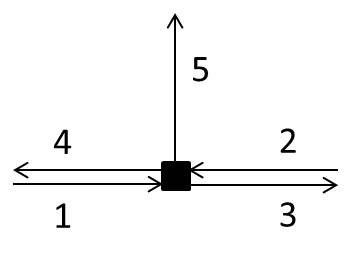
Figure 3: Intersection node.

Remark. As a rule of thumb, we suggest setting the restriction coefficient $\eta_{jj^{\prime}}^{i}$ equal to the portion of lanes serving movement $(i,j^{\prime})$ that also serve movement $(i,j)$. As an example, if movement $(i,j^{\prime})$ is served by four lanes, and of those lanes, one serves movement $(i,j)$, then a reasonable value for $\eta_{jj^{\prime}}^{i}$ is 0.25, as blockage of movement $(i,j)$ will block 25% of $(i,j^{\prime})$’s lanes.

Example. Recall our earlier example for a 4-by-4 junction during our discussion of the MIMO-with-FIFO node model in Section 3.2. Recall that our example supposed that the input links (see Figure 2 for the network topology) had capacity values of $F_{1}=F_{3}=1000$, and $F_{2}=F_{3}=2000$. Say that the links with capacity of 1000 are one-lane roads, while those links with capacity of 2000 are two-lane roads, with left and right turns permitted from one lane each, and the through movement permitted from both lanes. Following our rule of thumb, this would lead to a set of reduced mutual restriction coefficients:

$$\eta_{76}^{4} =\eta_{56}^{4}=0.5\qquad \eta_{75}^{4} =\eta_{57}^{4}=0$$

$$\eta_{58}^{2} =\eta_{78}^{2}=0.5 \eta_{75}^{2} =\eta_{57}^{2}=0$$

with all other restriction coefficients taking a value of 1. Let us examine the effect of our FIFO relaxation on this example. Since $C=1$, we ignore the index $c$ and perform some cancellations to clean up the notation.

$k=0:$ This iteration will proceed exactly as before, with $\tilde{U}(0)=\{1\}$ and flows from link 1 taking the demand value.

$k=1:$

1. $V(1)=\{5,6,7,8\}$

2. No changes are made to priorities for any $i\in\bigcup_{j\in V(1)}U_{j}(1)$.

3. No changes are made to oriented priorities.

4. $a_{5}(1)=2.92;\quad a_{6}(1)=1.83;\quad a_{7}(1)=0.685;\quad a_{8}(0)=0.723$
   $a_{j^{\ast}}(1)=a_{7}(1)=0.685$

5. $\tilde{U}(1)=\emptyset,$ as $\sum_{j}\tilde{S}_{2j}(1)=2000\nleq\tilde{p}_{2}(1)a_{7}(1)=1370$
   and $\sum_{j}\tilde{S}_{4j}(1)=1700\nleq\tilde{p}_{4}(1)a_{7}(1)=1370$

   • $\boldsymbol{f_{47}=\tilde{p}_{47}(1)a_{7}(1)=644.5}$

   • $\boldsymbol{f_{27}=\tilde{p}_{27}(1)a_{7}(1)=205.5}$

   • $\begin{aligned} \tilde{S}_{28}(2)&=(1-\eta_{78}^{2})S_{28}+\eta_{78}^{2}\times\nicefrac{{f_{27}}}{{S_{27}}}\times S_{28}\\ &=(1-0.5)\times 1600+0.5\times\nicefrac{{205.5}}{{300}}\times 1600\\ &=1348\end{aligned}$

   • $\begin{aligned} \tilde{S}_{46}(2)&=(1-\eta_{76}^{4})S_{46}+\eta_{76}^{4}\times\nicefrac{{f_{47}}}{{S_{47}}}\times S_{46}\\ &=(1-0.5)\times 800+0.5\nicefrac{{644.5}}{{800}}\times 800\\ &=722.25\end{aligned}$

   • $\tilde{R}_{7}(2)=850-644.5-204.5=0$

   • $U_{5}(2)=\{2,3,4\};\quad U_{6}(2)=\{3,4\};\quad U_{7}(2)=\emptyset;\quad U_{8}(2)=\{2,3\}$

$k=2:$

1. $V(2)=\{5,6,8\}$

2. No changes are made to priorities $p_{i}$.

3. Due to changes in two oriented demands, the new oriented priorities for input links 2 and 4 must be computed:

   • $\tilde{p}_{25}(2)=2000\times\nicefrac{{100}}{{1448}}=138.12$

   • $\tilde{p}_{28}(2)=2000\times\nicefrac{{1348}}{{1448}}=1861.9$

   • $\tilde{p}_{45}(2)=2000\times\nicefrac{{100}}{{822.25}}=243.24$

   • $\tilde{p}_{46}(2)=2000\times\nicefrac{{722.25}}{{822.25}}=1756.8$

4. The coefficients $a_{j}(2)$ are calculated with the new oriented priorities:

   • $a_{5}(2)=\frac{\tilde{R}_{5}(2)}{\tilde{p}_{25}(2)+\tilde{p}_{35}(2)+\tilde{p}_{45}(2)}=\frac{1000}{138.12+125+243.24}=1.92$

   • $a_{6}(2)=\frac{\tilde{R}_{6}(2)}{+\tilde{p}_{36}(2)+\tilde{p}_{46}(2)}=\frac{1950}{125+1756.8}=1.04$

   • $a_{8}(2)=\frac{\tilde{R}_{8}(2)}{+\tilde{p}_{28}(2)+\tilde{p}_{38}(2)}=\frac{1700}{1861.9+750}=0.651=a_{j^{\ast}}(2)$

5. $\tilde{U}(2)=\emptyset,$ as $\sum_{j}\tilde{S}_{2j}(2)=1448\nleq\tilde{p}_{2}(2)a_{8}(2)=1301$
   and $\sum_{j}\tilde{S}_{3j}(2)=800\nleq\tilde{p}_{3}(2)a_{8}(2)=651,$

   • $\boldsymbol{f_{28}=\tilde{p}_{28}(2)a_{8}(2)=1861.9\times 0.651=1211.75}$

   • $\boldsymbol{f_{38}=\tilde{p}_{38}(2)a_{8}(2)=750\times 0.651=488.25}$

   • $\eta_{85}^{2}=1,$ so $\boldsymbol{f_{25}=\tilde{p}_{25}(2)a_{8}(2)=138.12\times 0.651=89.916}$

   • $\eta_{85}^{3}=1,$ so $\boldsymbol{f_{35}=\tilde{p}_{35}(2)a_{8}(2)=125\times 0.651=81.375}$

   • $\eta_{86}^{3}=1,$ so $\boldsymbol{f_{36}=\tilde{p}_{36}(2)a_{8}(2)=125\times 0.651=81.375}$

   • $\tilde{R}_{5}(3)=1000-89.916-81.375=828.71;\quad\tilde{R}_{6}(3)=1950-81.375=1868.6$
     $\tilde{R}_{8}(3)=1700-1211.75-488.25=0$

   • $U_{5}(3)=\{4\};\quad U_{6}(3)=\{4\};\quad U_{8}(3)=\emptyset$

$k=3:$

1. $V(3)=\{5,6\}$

2. No changes are made to the priorities $p_{4}$, those of the only link $i$ remaining.

3. The oriented demands of link 4 remain the same as calculated in the previous iteration.

4. $a_{5}(3)=\nicefrac{{828.71}}{{258.39}}=3.21$
   $a_{6}(3)=\nicefrac{{1861.6}}{{1741.6}}=1.073=a_{j^{\ast}}(3)$

5. $\tilde{U}(3)=\{4\}$, as $\sum_{j}\tilde{S}_{4j}=774\leq\tilde{p}_{4}(3)a_{6}(3)=2146$
   $\boldsymbol{f_{45}=\tilde{S}_{45}(3)=100;}\quad\boldsymbol{f_{46}=\tilde{S}_{46}(3)=722.25}$
   $U_{j}(4)=\emptyset\quad\forall j$

$k=4:$

1. $V(4)=\emptyset$, so the algorithm terminates. All flows have been found.

Comparison of the resulting flows with those from the non-relaxed FIFO example illustrates several differences caused by this relaxation. Unsurprisingly, the two-lane links (2 and 4) that take advantage of the FIFO relaxation send greater amounts of vehicles to links 5, 6 and 8. Previously, these flows had been cut off by the filling of link 7’s supply. Perhaps more interesting is the effect on the flows of link 3. In the previous example, link 3 was able to send vehicles equal to its demand, since there was enough leftover supply in link 8 after the flow $f_{28}$ was constrained by FIFO. In our example with relaxed FIFO, however, link 8 had more supply consumed by the higher-priority link 2, and it was found that link 3 was unable to send its entire demand. Since we had assumed that link 3 was a one-lane road and thus bounded by FIFO, this restricted its other flows as well.

In both cases, link 3 was lower priority than link 2 and was disadvantaged in claiming link 8’s supply, but qualitatively, permitting a FIFO relaxation for the two-lane roads exacerbated the “advantage” they already had over the one-lane roads (from having priority equal to capacity).

The main result of this Section can be stated as the following theorem.

Theorem 3.5.

Given a set of input links $i\in 1,\dots,M$, output links $j\in 1,\dots,N$, commodities $c\in 1,\dots,C$, priorities $p_{i}$, split ratios $\beta_{i}$, and mutual restriction coefficients $\{\eta_{j,j^{\prime}}^{i}\}$, the algorithm of Section 3.5 obtains the unique solution of the optimization problem (3.20)-(3.24), (3.26), (3.39).

Proof.

The priority constraint (3.26) makes this optimization problem non-convex, except in the above-mentioned special case where $N=1$ and the priorities $p_{i}$ are taken as proportional to the send functions. Recall our discussion in Section 3.2 that the priority constraint must be replaced entirely with the unrealistic constraint 3.27 to obtain an LP. Our priority constraint increases the complexity of the problem significantly. In fact, we conjecture that in the MIMO case, both with and without relaxation of the FIFO constraint, there is no way to verify a solution faster than re-solving the problem (3.20)-(3.24), (3.26), (3.39). Thus, we will prove optimality by showing that as our algorithm proceeds through iterations, it constructs the unique optimal solution.

We may decompose the problem into finding the $M\cdot N\cdot C$ interrelated quantities $\{f_{ij}^{c}\}$. The $C$ flows for each $(i,j)$ are further constrained by our commodity flow proportionality constraint (3.24); solving for one of $\{f_{ij}^{1},\dots,f_{ij}^{C}\}$ also constrains them all. Our task then becomes finding optimal values for each of $M\cdot N$ subsets $\{f_{ij}^{1},\dots,f_{ij}^{C}\}$. Our algorithm finds at least one of these $M\cdot N$ subsets per iteration $k$. The assignments are done by either equation (3.41) or equation (3.42). Over iterations, subsets are assigned to build up the unique optimum solution. We can show that each subset assigned is optimal; that is, at least one of the constraints is tight.

Let us first consider formulae (3.43)-(3.44), our implementation of the relaxed FIFO constraint. In step 5 of our algorithm, we identify a single output link as $j^{\ast}$. The argmin in this step picks out a single link as the most restrictive of all output links. By the relaxed FIFO construction, all $i\in U_{j^{\ast}}$ will feel a relaxed FIFO effect instigated by $j^{\ast}$ as the most restrictive link. For a generic $j\neq j^{\ast}$, equation (3.44) enforces the relaxed FIFO constraint by decaying the oriented demand $\tilde{S}_{ij}$. In fact, this oriented demand acts as a proxy for the restricted FIFO constraint. Since a $f_{ij}^{c}$ that is restricted by relaxed FIFO will, by construction, never obtain $f_{ij}^{c}=S_{ij}^{c}$, the running quantity $S_{ij}^{c}(k)$ represents an “effective” oriented demand after application of restricted FIFO. If it turns out that a flow is found $f_{ij}^{c}=\tilde{S}_{ij}^{c}(k)\leq S_{ij}^{c}$ for some $k$, then this flow value has an active constraint imposed by relaxed FIFO.

Now consider flows assigned by equation (3.42). In the special case where $j=j^{\ast}$, we have

$$\sum_{c=1}^{C}\sum_{i\in U_{j^{\ast}}(k)}f_{ij^{\ast}}^{c} =\sum_{c=1}^{C}\sum_{i\in U_{j^{\ast}}(k)}\tilde{S}_{ij^{\ast}}(k)\frac{\tilde{p}_{ij^{\ast}}(k)a_{j^{\ast}}(k)}{\sum_{c^{\prime}=1}^{C}\tilde{S}_{ij^{\ast}}^{c^{\prime}}(k)}$$

$$=\sum_{i\in U_{j^{\ast}}(k)}\tilde{p}_{ij^{\ast}}(k)a_{j^{\ast}}(k)$$

$$=\left(\sum_{i\in U_{j^{\ast}}(k)}\tilde{p}_{ij^{\ast}}(k)\right)\frac{\tilde{R}_{j^{\ast}}(k)}{\sum_{i\in U_{j^{\ast}}(k)}\tilde{p}_{ij^{\ast}}(k)}$$

$$=\tilde{R}_{j^{\ast}}(k),$$

so all the flows into link $j^{\ast}$ take up all available supply. These flows are thus constrained by the supply constraint, (3.23).

For flows assigned by equation (3.42) in the case of $j\neq j^{\ast}$, we have $i\in U_{j^{\ast}}$, and a restriction coefficient $\eta_{j^{\ast}j}^{i}=1$ that implies a strict FIFO constraint. In other words, we need

$$\frac{\sum_{c=1}^{C}f_{ij}^{c}}{\sum_{c=1}^{C}\left(f_{ij}^{c}+f_{ij^{\ast}}^{c}\right)}=\frac{\sum_{c=1}^{C}\tilde{S}_{ij}^{c}(k)}{\sum_{c=1}^{C}\left(\tilde{S}_{ij}^{c}(k)+\tilde{S}_{ij^{\ast}}^{c}(k)\right)}.$$

Examining the denominator of the LHS, we can write

$$\sum_{c=1}^{C}f_{ij}^{c}+f_{ij^{\ast}}^{c} =\sum_{c=1}^{C}\left(\tilde{p}_{ij}^{c}(k)+\tilde{p}_{ij^{\ast}}^{c}(k)\right)a_{j^{\ast}}(k)$$

$$=\sum_{c=1}^{C}\frac{\tilde{p}_{i}(k)}{\sum_{j\in V(k)}\tilde{S}_{ij}^{c}(k)}\left(\tilde{S}_{ij}(k)+\tilde{S}_{ij^{\ast}}(k)\right)a_{j^{\ast}}(k).$$

Straightforward algebra then gives

$$\frac{\sum_{c=1}^{C}f_{ij}^{c}}{\sum_{c=1}^{C}\left(f_{ij}^{c}+f_{ij^{\ast}}^{c}\right)} =\sum_{c=1}^{C}\frac{\tilde{p}_{i}(k)}{\tilde{p}_{i}(k)}\times\frac{\tilde{S}_{ij}^{c}(k)}{\tilde{S}_{ij}^{c}(k)+\tilde{S}_{ij^{\ast}}^{c}(k)}\times\frac{\sum_{j\in V(k)}\tilde{S}_{ij}^{c}(k)}{\sum_{j\in V(k)}\tilde{S}_{ij}^{c}(k)}\times\frac{a_{j^{\ast}}(k)}{a_{j^{\ast}}(k)}$$

$$=\frac{\sum_{c=1}^{C}\tilde{S}_{ij}^{c}(k)}{\sum_{c=1}^{C}\left(\tilde{S}_{ij}^{c}(k)+\tilde{S}_{ij^{\ast}}^{c}(k)\right)}.$$

as originally required. Thus, flows $\{f_{ij}^{c}\},j\neq j^{\ast}$ assigned in equation (3.42) are constrained by the strict FIFO constraint, (3.39) with $\eta_{j^{\ast}j}^{i}=1$.

For flows assigned by equation (3.41), we have for each flow $i$, $f_{ij}^{c}=\tilde{S}_{ij}^{c}(k)$, so these flows are constrained by (3.22).

Uniqueness of the solution is equivalent to showing that we must assign flows in the order described. That is, that flows for the most restrictive link $j^{\ast}$ should be assigned at iteration $k$. It turns out that setting the flows of any other $j\neq j^{\ast}$ may produce solutions that violate the problem constraints. At iteration $k$, let $j^{\prime}$ be some other constrained outgoing link, with $a_{j^{\ast}}(k)<a_{j^{\prime}}(k)$, and let $i^{\prime}$ be any input link in $U_{j^{\ast}}(k)\cap U_{j^{\prime}}(k)$. Proceeding through our algorithm, we will obtain an upper bound on the sum of flows from $i^{\prime}$ to $j^{\prime}$ through the restriction coefficient:

$$\sum_{c=1}^{C}f_{i^{\prime}j^{\prime}}^{c} \leq\min\left\{\tilde{S}_{i^{\prime}j^{\prime}}(k+1),\tilde{p}_{i^{\prime}}(k+1)a_{j^{\prime}}(k+1)\right\}$$

$$\leq\tilde{S}_{i^{\prime}j^{\prime}}(k+1)$$

$$\leq(1-\eta_{j^{\ast}j^{\prime}}^{i^{\prime}})\sum_{c=1}^{C}S_{i^{\prime}j^{\prime}}^{c}+\eta_{j^{\ast}j^{\prime}}^{i^{\prime}}\frac{\sum_{c=1}^{C}f_{i^{\prime}j^{\ast}}^{c}}{\sum_{c=1}^{C}S_{i^{\prime}j^{\ast}}^{c}}\sum_{c=1}^{C}S_{i^{\prime}j^{\prime}}^{c}\triangleq\overline{f_{i^{\prime}j^{\prime}}}.$$

Suppose instead that we had decided to set flows into $j^{\prime}$ at iteration $k$. Then we would have

$$\sum_{c=1}^{C}f_{i^{\prime}j^{\prime}}^{c} =\tilde{p}_{i^{\prime}j^{\prime}}(k)a_{j^{\ast}}(k)=\frac{\tilde{p}_{i^{\prime}j^{\prime}}(k)}{\sum_{i\in U_{j^{\prime}}(k)}\tilde{p}_{i^{\prime}j^{\prime}}(k)}\tilde{R}_{j^{\prime}}(k).$$ (3.45)

Note that (3.45) does not make use of the restriction coefficient $\eta_{j^{\ast}j^{\prime}}^{i^{\prime}}$, and therefore does not take (relaxed) FIFO into consideration. In fact, for a suitably large $\eta_{j^{\ast}j^{\prime}}^{i^{\prime}}$ and/or small ratio $\frac{\sum_{c=1}^{C}f_{i^{\prime}j^{\ast}}^{c}}{\sum_{c=1}^{C}S_{i^{\prime}j^{\ast}}^{c}}$, we can obtain

$$\frac{\tilde{p}_{i^{\prime}j^{\prime}}(k)}{\sum_{i\in U_{j^{\prime}}(k)}\tilde{p}_{i^{\prime}j^{\prime}}(k)}\tilde{R}_{j^{\prime}}(k) >\left(\eta_{j^{\ast}j^{\prime}}^{i^{\prime}}\frac{\sum_{c=1}^{C}f_{i^{\prime}j^{\ast}}^{c}}{\sum_{c=1}^{C}S_{i^{\prime}j^{\ast}}^{c}}+1-\eta_{j^{\ast}j^{\prime}}^{i^{\prime}}\right)\sum_{c=1}^{C}S_{i^{\prime}j^{\prime}}^{c}$$

$$\sum_{c=1}^{C}f_{i^{\prime}j^{\prime}}^{c} >\overline{f_{i^{\prime}j^{\prime}}},$$

breaking our upper bound imposed by (relaxed) FIFO (3.39). ∎

Corollary 3.1.

Theorems 3.1, 3.2, and 3.4 follow from the Theorem 3.5 as special cases.

Remark. It was discussed above that the Tampére et al. node models are special cases of this node model (with all $\eta^{i}_{jj^{\prime}}=1$ and certain choices of $p_{i}$). The above proof then also applies to the similar theorem for that model.

4 Node with Undefined Split Ratios: Traffic Assignment

In this section we consider a MIMO node with $M$ input links, $N$ output links and $C$ commodities, where some of the split ratios $\beta_{ij}^{c}$ are not defined a priori and must be computed as functions of the input demand $S_{i}^{c}$, priorities $p_{i}$ and the output supply $R_{j}$, $i=1,\dots,M$, $j=1,\dots,N$ and $c=1,\dots,C$. This may occur if the modeler chooses to let drivers at a node select a route to their destination in response to changing conditions; a specific example of such a node is given in an example describing an interchange between a freeway and a managed lane to be discussed after presentation of the algorithm. Here we present the algorithm for computing undefined split ratios based on the following definitions and assumptions:

• Define the set of commodity movements, for which split ratios are known, ${\cal B}=\left\{\left\{i,j,c\right\}:\;\beta_{ij}^{c}\in[0,1]\right\}$, and the set of commodity movements, for which split ratios are to be computed, $\overline{{\cal B}}=\left\{\left\{i,j,c\right\}:\;\beta_{ij}^{c}\mbox{ are unknown}\right\}$.

• For a given input link $i$ and commodity $c$ such that $S_{i}^{c}=0$, assume that all split ratios are known: $\{i,j,c\}\in{\cal B}$.

• Define the set of output links, for which there exist unknown split ratios, $V=\left\{j:\;\exists\left\{i,j,c\right\}\in\overline{{\cal B}}\right\}$.

• Assuming that for a given input link $i$ and commodity $c$ split ratios must sum up to 1, define the unassigned portion of flow $\overline{\beta}_{i}^{c}=1-\sum_{j:\{i,j,c\}\in{\cal B}}\beta_{ij}^{c}$.

• For a given input link $i$ and commodity $c$ such that there exist $\{i,j,c\}\in\overline{{\cal B}}$, assume $\overline{\beta}_{i}^{c}>0$, otherwise the undefined split ratios can be trivially set to 0.

• For every output link $j\in V$, define the set of input links that have an unassigned demand portion directed toward this output link, $U_{j}=\left\{i:\;\exists\left\{i,j,c\right\}\in\overline{{\cal B}}\right\}$.

• For a given input link $i$ and commodity $c$ define the set of output links, split ratios for which are to be computed, $V_{i}^{c}=\left\{j:\;\exists i\in U_{j}\right\}$, and assume that if nonempty, this set contains at least two elements, otherwise a single split ratio can be trivially set to $\overline{\beta}_{i}^{c}$.

• Assume that input link priorities are nonnegative, $p_{i}\geq 0$, $i=1,\dots,M$, and $\sum_{i=1}^{M}p_{i}=1$. Note that, although in section 3 we did not require the input priorities to sum to one, in this section we assume this normalization is done to simplify the notation.

• Define the set of input links with zero priority: $U_{zp}=\left\{i:\;p_{i}=0\right\}$. To avoid dealing with zero input priorities, perform regularization:

  $$\tilde{p}_{i}=p_{i}\left(1-\frac{|U_{zp}|}{M}\right)+\frac{1}{M}\frac{|U_{zp}|}{M}=p_{i}\frac{M-|U_{zp}|}{M}+\frac{|U_{zp}|}{M^{2}},$$ (4.1)

  where $|U_{zp}|$ denotes the number of elements in set $U_{zp}$. Expression (4.1) implies that the regularized input priority $\tilde{p}_{i}$ consists of two parts: (1) the original input priority $p_{i}$ normalized to the portion of input links with nonzero priorities; and (2) uniform distribution among $M$ input links, $\frac{1}{M}$, normalized to the portion of input links with zero priorities.

  Note that $\tilde{p}_{i}\geq 0$, $i=1,\dots,M$, and $\sum_{i=1}^{M}\tilde{p}_{i}=1$.

The algorithm for distributing $\overline{\beta}_{i}^{c}$ among the commodity movements in $\overline{{\cal B}}$, that is assigning values to the a priori unknown split ratios, aims at maintaining output links as uniformly occupied as possible. It is described next.

1. Initialize:

   $$\tilde{\beta}_{ij}^{c}(0) := \left\{\begin{array}[]{ll}\beta_{ij}^{c},&\mbox{ if }\{i,j,c\}\in{\cal B},\\ 0,&\mbox{ otherwise};\end{array}\right.$$

   $$\overline{\beta}_{i}^{c}(0) := \overline{\beta}_{i}^{c};$$

   $$\tilde{U}_{j}(0) = U_{j};$$

   $$\tilde{V}(0) = V;$$

   $$k := 0,$$

   Here $\tilde{U}_{j}(k)$ is the remaining set of input links with some unassigned demand, which may be directed to output link $j$; and $\tilde{V}(k)$ is the remaining set of output links, to which the still unassigned demand may be directed.

2. If $\tilde{V}(k)=\emptyset$, stop. The sought-for split ratios are $\left\{\tilde{\beta}_{ij}^{c}(k)\right\}$, $i=1,\dots,M$, $j=1,\dots,N$, $c=1,\dots,C$.

3. Calculate the remaining unallocated demand:

   $$\overline{S}_{i}^{c}(k)=\overline{\beta}_{i}^{c}(k)S_{i}^{c},\;\;\;i=1,\dots,M,\;\;c=1,\dots,C.$$

4. For all input-output link pairs calculate oriented demand analogously to (3.18):

   $$\tilde{S}_{ij}^{c}(k)=\tilde{\beta}_{ij}^{c}(k)S_{i}^{c}.$$

5. For all input-output link pairs calculate oriented priorities:

   $$\tilde{p}_{ij}(k) = \tilde{p}_{i}\frac{\sum_{c=1}^{C}\gamma_{ij}^{c}S_{i}^{c}}{\sum_{c=1}^{C}S_{i}^{c}}$$ (4.3)

   with

   $$\gamma_{ij}^{c}(k) = \left\{\begin{array}[]{ll}\beta_{ij}^{c},&\mbox{ if split ratio is defined a priori: }\{i,j,c\}\in{\cal B},\\ \tilde{\beta}_{ij}^{c}(k)+\frac{\overline{\beta}_{i}^{c}(k)}{|V_{i}^{c}|},&\mbox{ otherwise},\end{array}\right.$$ (4.6)

   where $|V_{i}^{c}|$ denotes the number of elements in the set $V_{i}^{c}$. Comparing the expression (4.3)-(4.6) with (3.29), one can see that split ratios $\tilde{\beta}_{ij}^{c}(k)$, which are not fully defined yet, are complemented with a fraction of $\overline{\beta}_{i}^{c}(k)$ inversely proportional to the number of output links among which the flow of commodity $c$ from input link $i$ can be distributed.

   Note that in this step we user regularized priorities $\tilde{p}_{i}$ as opposed to the original $p_{i}$, $i=1,\dots,M$. This is done to ensure that inputs with $p_{i}=0$ are not ignored in the split ratio assignment.

6. Find the largest oriented demand-supply ratio:

   $$\mu^{+}(k)=\max_{j}\max_{i}\frac{\sum_{c=1}^{C}\tilde{S}_{ij}^{c}(k)}{\tilde{p}_{ij}(k)R_{j}}\sum_{i\in U_{j}}\tilde{p}_{ij}(k).$$

7. Define the set of all output links, where the minimum of the oriented demand-supply ratio is achieved:

   $$Y(k)=\arg\min_{j\in\tilde{V}(k)}\min_{i\in\tilde{U}_{j}(k)}\frac{\sum_{c=1}^{C}\tilde{S}_{ij}^{c}(k)}{\tilde{p}_{ij}(k)R_{j}}\sum_{i\in U_{j}}\tilde{p}_{ij}(k),$$

   and from this set pick the output link $j^{-}$ with the smallest output demand-supply ratio is minimal (when there are multiple minimizing output links, any of the minimizing output links may be chosen as $j^{-}$):

   $$j^{-}=\arg\min_{j\in Y(k)}\frac{\sum_{i=1}^{M}\sum_{c=1}^{C}\tilde{S}_{ij}^{c}(k)}{R_{j}}.$$

8. Define the set of all input links, where the minimum of the oriented demand-supply ratio for the output link $j^{-}$ is achieved:

   $$W_{j^{-}}(k)=\arg\min_{i\in\tilde{U}_{j^{-}}(k)}\frac{\sum_{c=1}^{C}\tilde{S}_{ij^{-}}^{c}(k)}{\tilde{p}_{ij^{-}}(k)R_{j^{-}}}\sum_{i\in U_{j^{-}}}\tilde{p}_{ij^{-}}(k),$$

   and from this set pick the input link $i^{-}$ and commodity $c^{-}$ with the smallest remaining unallocated demand:

   $$\{i^{-},c^{-}\}=\arg\min_{\begin{array}[]{c}i\in W_{j^{-}}(k),\\ c:\overline{\beta}_{i^{-}}^{c}(k)>0\end{array}}\overline{S}_{i}^{c}(k).$$

9. Define the smallest oriented demand-supply ratio:

   $$\mu^{-}(k)=\frac{\sum_{c=1}^{C}\tilde{S}_{i^{-}j^{-}}^{c}(k)}{\tilde{p}_{i^{-}j^{-}}(k)R_{j^{-}}}\sum_{i\in U_{j^{-}}}\tilde{p}_{ij-}(k).$$

   • If $\mu^{-}(k)=\mu^{+}(k)$, which means that the oriented demand is perfectly balanced among the output links, distribute the unassigned demand proportionally to the allocated supply:

     $$\tilde{\beta}_{i^{-}j}^{c^{-}}(k+1) = \tilde{\beta}_{i^{-}j}^{c^{-}}(k)+\frac{\tilde{p}_{i^{-}j}(k)R_{j}}{\sum_{j^{\prime}\in\tilde{V}_{i^{-}}^{c^{-}}(k)}\tilde{p}_{i^{-}j^{\prime}}(k)R_{j^{\prime}}}\overline{\beta}_{i^{-}}^{c^{-}}(k),\;\;\;j\in\tilde{V}_{i^{-}}^{c^{-}}(k);$$ (4.7)

     $$\tilde{\beta}_{ij}^{c}(k+1) = \tilde{\beta}_{ij}^{c}(k)\mbox{ for }\{i,j,c\}\neq\{i^{-},j,c^{-}\};$$ (4.8)

     $$\overline{\beta}_{i^{-}}^{c^{-}}(k+1) = 0;$$

     $$\overline{\beta}_{i}^{c}(k+1) = \overline{\beta}_{i}^{c}(k)\mbox{ for }\{i,c\}\neq\{i^{-},c^{-}\}.$$

   • Else, assign:

     $$\Delta\tilde{\beta}_{i^{-}j^{-}}^{c^{-}}(k) = \min\left\{\overline{\beta}_{i^{-}}^{c^{-}}(k),\;\;\left(\frac{\mu^{+}(k)\tilde{p}_{i^{-}j^{-}}(k)R_{j^{-}}}{\overline{S}_{i^{-}}^{c^{-}}(k)\sum_{i\in U_{j^{-}}}\tilde{p}_{ij^{-}}(k)}-\frac{\sum_{c=1}^{C}\tilde{S}_{i^{-}j^{-}}^{c}(k)}{\overline{S}_{i^{-}}^{c^{-}}(k)}\right)\right\};$$ (4.9)

     $$\tilde{\beta}_{i^{-}j^{-}}^{c^{-}}(k+1) = \tilde{\beta}_{i^{-}j^{-}}^{c^{-}}(k)+\Delta\tilde{\beta}_{i^{-}j^{-}}^{c^{-}}(k);$$ (4.10)

     $$\tilde{\beta}_{ij}^{c}(k+1) = \tilde{\beta}_{ij}^{c}(k)\mbox{ for }\{i,j,c\}\neq\{i^{-},j^{-},c^{-}\};$$ (4.11)

     $$\overline{\beta}_{i^{-}}^{c^{-}}(k+1) = \overline{\beta}_{i^{-}}^{c^{-}}(k)-\Delta\tilde{\beta}_{i^{-}j^{-}}^{c^{-}}(k);$$

     $$\overline{\beta}_{i}^{c}(k+1) = \overline{\beta}_{i}^{c}(k)\mbox{ for }\{i,c\}\neq\{i^{-},c^{-}\}.$$

10. Update sets $\tilde{U}_{j}(k)$ and $\tilde{V}(k)$:

    $$\tilde{U}_{j}(k+1) = \tilde{U}_{j}(k)\setminus\left\{i^{-}:\;\overline{\beta}_{i^{-}}^{c}(k+1)=0,\;c=1,\dots,C\right\},\;\;\;j\in\tilde{V}(k);$$

    $$\tilde{V}(k+1) = \tilde{V}(k)\setminus\left\{j:\;\tilde{U}_{j}(k+1)=\emptyset\right\}.$$

11. Set $k:=k+1$ and return to step 2.

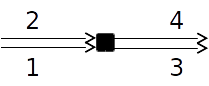
Figure 4: Merge-diverge intersection example.

Example. Consider the node presented in Figure 4. The node represents a junction between two parallel links, or a merge-diverge. Nodes such of these may be used to model locations where drivers can choose to shift between two parallel roads or lane groups; the canonical example is an access point for a managed lane facility adjacent to a freeway, where drivers may choose to enter or exit the managed lane. In this example, we will say that links 1 and 3 represent a freeway’s general purpose (GP) lanes, and links 2 and 4 represent a high-occupancy vehicle (HOV) lane, open only to a select group of vehicles. The Low-Occupancy Vehicles (LOVs) and HOVs will be modeled as separate commodities, with notations of $L$ for LOVs and $H$ for HOVs.

Suppose we have input parameters of:

$\beta_{14}^{L}=0$	$\beta_{13}^{L}=1$
$\beta_{14}^{H}=?$	$\beta_{13}^{H}=?$	$p_{1}=\nicefrac{{3}}{{4}}$
$\beta_{23}^{H}=?$	$\beta_{24}^{H}=?$	$p_{2}=\nicefrac{{1}}{{4}}$
$S_{1}^{L}=500$	$S_{1}^{H}=100$	$R_{3}=600$
$S_{2}^{H}=50$		$R_{4}=200$

In words, the LOVs are not allowed to enter the HOV lane; HOVs are allowed, but individual vehicles may or may not choose to do so: both links can bring them to their eventual downstream destination so the choice of link to take will be made in response to immediate local congestion conditions.

Let us see how algorithm would assign split ratios for the HOVs.

$k=0:$

1. $\tilde{\beta}_{13}^{H}(0)=\tilde{\beta}_{14}^{H}(0)=\tilde{\beta}_{23}^{H}(0)=\tilde{\beta}_{24}^{H}(0)=0$
   $\overline{\beta}_{3}^{H}(0)=\overline{\beta}_{4}^{H}(0)=1$
   $\tilde{U}_{3}(0)=\tilde{U}_{4}(0)=\{1,2\};\qquad\tilde{V}(0)=\{3,4\}$

2. $\tilde{V}(0)=\{3,4\}\neq\emptyset$, the algorithm proceeds.

3. $\overline{S}^{H}_{1}(0)=100,\qquad\overline{S}^{H}_{2}(0)=50,\qquad\overline{S}_{1}^{L}(0)=0$

4. $\tilde{S}_{13}^{L}(0)=500;\qquad\tilde{S}_{13}^{H}(0)=\tilde{S}_{14}^{H}(0)=\tilde{S}_{23}^{H}(0)=\tilde{S}_{24}^{H}(0)=0$

5. $\gamma_{13}^{H}=\gamma_{14}^{H}=\nicefrac{{1}}{{2}};\qquad\gamma_{23}^{H}=\gamma_{24}^{H}=\nicefrac{{1}}{{2}};\qquad\gamma_{13}^{L}=1$

   $\begin{aligned} \tilde{p}_{13}(0)&=\frac{\tilde{p}_{1}\left(\gamma_{13}^{H}S_{1}^{H}+\gamma_{13}^{L}S_{1}^{L}\right)}{S_{1}^{H}+S_{1}^{L}}=\frac{\nicefrac{{3}}{{4}}\left(\nicefrac{{1}}{{2}}\times 100+1\times 500\right)}{100+500}=0.6875\\ \tilde{p}_{14}(0)&=\frac{\nicefrac{{3}}{{4}}\left(\nicefrac{{1}}{{2}}\times 100+0\times 500\right)}{100+500}=0.0625\\ \tilde{p}_{23}(0)&=\frac{\nicefrac{{1}}{{4}}\left(\nicefrac{{1}}{{2}}\times 50\right)}{50}=0.125\\ \tilde{p}_{24}(0)&=0.125\end{aligned}$

6. $\begin{aligned} \mu^{+}(0)=\frac{\tilde{S}_{13}^{L}(0)+\tilde{S}_{13}^{H}(0)}{\tilde{p}_{13}(0)R_{3}}\sum_{i\in U_{3}}\tilde{p}_{i3}(0)=0.9848\end{aligned}$, for all other pairs the ratio equals 0.

7. $Y(0)=\{3,4\};$
   $j^{-}=4$

8. $W_{4}(0)=\{1,2\}$, as there are no oriented demands to link 4 as of yet.
   $(i^{-},c^{-})=(2,H)$

9. $\mu^{-}(0)=0$

   $\begin{aligned} \Delta\tilde{\beta}_{i^{-}j^{-}}^{c^{-}}(0)&=\Delta\tilde{\beta}_{24}^{H}(0)=\min\left\{1,\left(\frac{0.9848\times 0.125\times 200}{50\times 0.1875}-\frac{0}{50}\right)\right\}=\min\left\{1,2.616\right\}=1\\ \tilde{\beta}_{24}^{H}(1)&=0+1=1\\ \overline{\beta}_{2}^{H}(1)&=1-0=0\end{aligned}$

10. $\tilde{U}_{3}(1)=\tilde{U}_{4}(1)=\{1\};\qquad\tilde{V}(1)=\{3,4\}$

$k=1:$

1. $\tilde{V}(1)=\{3,4\}$

2. $\overline{S}_{1}^{H}(1)=100,\qquad\overline{S}^{H}_{2}(1)=0,\qquad\overline{S}_{1}^{L}(1)=0$

3. $\tilde{S}_{13}^{L}(0)=500;\qquad\tilde{S}_{13}^{H}(1)=\tilde{S}_{14}^{H}(1)=\tilde{S}_{23}^{H}(1)=0;\qquad\tilde{S}_{24}^{H}(1)=50$

4. $\gamma_{13}^{H}=\gamma_{14}^{H}=\nicefrac{{1}}{{2}};\qquad\gamma_{23}^{H}=0;\qquad\gamma_{24}^{H}=1;\qquad\gamma_{13}^{L}=1$
   $\tilde{p}_{13}(1)=0.6875;\qquad\tilde{p}_{14}(1)=0.0625;$
   $\tilde{p}_{23}(1)=0;\qquad\tilde{p}_{24}(1)=0.25$

5. $\begin{aligned} &\frac{\tilde{S}_{13}^{L}(1)+\tilde{S}_{13}^{H}(1)}{\tilde{p}_{13}(1)R_{3}}\sum_{i\in U_{3}}\tilde{p}_{i3}(1)=0.8333=\mu^{+}(1)\\ &\frac{\tilde{S}_{24}^{L}(1)+\tilde{S}_{24}^{H}(1)}{\tilde{p}_{24}(1)R_{4}}\sum_{i\in U_{4}}\tilde{p}_{i4}(1)=0.3125\end{aligned}$

   For the two other pairs the ratio equals 0.

6. $Y(1)=\{4\};$
   $j^{-}=4$

7. $W_{4}(1)=\{1\}$
   $(i^{-}c^{-})=(1,H)$

8. $\mu^{-}(1)=0$

   $\begin{aligned} \Delta\tilde{\beta}_{i^{-}j^{-}}^{c^{-}}(1)&=\Delta\tilde{\beta}_{14}^{H}(1)=\min\left\{1,\left(\frac{0.8333\times 0.0625\times 200}{100\times 0.3125}-\frac{0}{100}\right)\right\}=\min\left\{1,\nicefrac{{1}}{{3}}\right\}=\nicefrac{{1}}{{3}}\\ \tilde{\beta}_{14}^{H}(2)&=0+\nicefrac{{1}}{{3}}=\nicefrac{{1}}{{3}}\\ \overline{\beta}_{2}^{H}(2)&=1-\nicefrac{{1}}{{3}}=\nicefrac{{2}}{{3}}\end{aligned}$

9. $\tilde{U}_{3}(2)=\tilde{U}_{4}(2)=\{1\};\qquad\tilde{V}(2)=\{3,4\}$

$k=2:$

1. $\tilde{V}(2)=\{3,4\}$

2. $\overline{S}_{1}^{H}(2)=66.67,\qquad\overline{S}^{H}_{2}(2)=0,\qquad\overline{S}_{1}^{L}(2)=0$

3. $\tilde{S}_{13}^{L}(2)=500;\qquad\tilde{S}_{24}^{H}(2)=50;\qquad\tilde{S}_{14}^{H}(2)=33.33;\qquad\tilde{S}_{13}^{H}(2)=\tilde{S}_{23}^{H}(2)=0$

4. $\gamma_{13}^{H}=\nicefrac{{1}}{{3}};\qquad\gamma_{14}^{H}=\nicefrac{{2}}{{3}};\qquad\gamma_{23}^{H}=0;\qquad\gamma_{24}^{H}=1;\qquad\gamma_{13}^{L}=1$
   $\tilde{p}_{13}(2)=\nicefrac{{2}}{{3}};\qquad\tilde{p}_{14}(2)=\nicefrac{{1}}{{12}};$
   $\tilde{p}_{23}(2)=0;\qquad\tilde{p}_{24}(2)=0.25$

5. $\begin{aligned} &\frac{\tilde{S}_{13}^{L}(2)+\tilde{S}_{13}^{H}(2)}{\tilde{p}_{13}(2)R_{3}}\sum_{i\in U_{3}}\tilde{p}_{i3}(2)=0.8333=\mu^{+}(2)\\ &\frac{\tilde{S}_{14}^{L}(2)+\tilde{S}_{14}^{H}(2)}{\tilde{p}_{14}(2)R_{4}}\sum_{i\in U_{4}}\tilde{p}_{i4}(2)=0.6667\\ &\frac{\tilde{S}_{23}^{L}(2)+\tilde{S}_{23}^{H}(2)}{\tilde{p}_{23}(2)R_{3}}\sum_{i\in U_{3}}\tilde{p}_{i3}(2)=0\\ &\frac{\tilde{S}_{24}^{L}(2)+\tilde{S}_{24}^{H}(2)}{\tilde{p}_{24}(2)R_{4}}\sum_{i\in U_{4}}\tilde{p}_{i4}(2)=0.3333\end{aligned}$

6. $Y(2)=\{3\};$
   $j^{-}=3$

7. $W_{3}(2)=\{1\}$
   $(i^{-}c^{-})=(1,H)$

8. $\mu^{-}(2)=0.8333=\mu^{+}(2)$

   $\begin{aligned} \tilde{\beta}_{13}^{H}(3)&=0+\frac{\nicefrac{{2}}{{3}}\times 600}{\nicefrac{{2}}{{3}}\times 600+\nicefrac{{1}}{{12}}\times 200}\times\nicefrac{{2}}{{3}}=0+0.96\times\nicefrac{{2}}{{3}}=0.64\\ \tilde{\beta}_{23}^{H}(3)&=\nicefrac{{1}}{{3}}+\frac{\nicefrac{{1}}{{12}}\times 200}{\nicefrac{{2}}{{3}}\times 600+\nicefrac{{1}}{{12}}\times 200}\times\nicefrac{{2}}{{3}}=\nicefrac{{1}}{{3}}+0.04\times\nicefrac{{2}}{{3}}=0.36\\ \overline{\beta}_{1}^{H}(3)&=\nicefrac{{2}}{{3}}-0.64-0.0267=0\end{aligned}$

9. $\tilde{U}_{3}(3)=\tilde{U}_{4}(3)=\emptyset;\qquad\tilde{V}(3)=\emptyset$

$k=3:$

1. $\tilde{V}(3)=\emptyset$

The algorithm terminates. The resulting split ratios are $\boldsymbol{\beta_{13}^{H}=0.64,\quad\beta_{23}^{H}=0.36,\quad\beta_{24}^{H}=1,\quad\beta_{23}^{H}=0}$.

5 Conclusion

This paper introduced the first order macroscopic traffic model, LNCTM, for modeling multi-commodity traffic on road networks. An example of the LNCTM application is the freeway network with special lanes, where different vehicle classes have different permissions to enter those special lanes.

One of the features of the LNCTM is the fundamental diagram in the shape of the “inverse lambda” that allows modeling of the capacity drop and a hysteresis behavior of the traffic state in a link that goes from free flow to congestion and back (Section 2).

The cornerstone of the LNCTM is the model of a node with multiple input and multiple output links, which computes traffic flows per commodity from input to output links and is governed by the input demand, output supply, split ratios that define how incoming flows must be distributed between output links, and input link priorities that define the output supply allocation for incoming flows (Sections 3.1-3.2). The proposed node model accepts arbitrary input link priorities, and it is shown that the node model presented in Tampère et al. (2011) is the special case of the proposed node model when input link priorities are proportional to input link capacities (Sections 3.3). We also analyzed the non-convex nature of the node model, showing its difference from the Bliemer node model (Bliemer, 2007) that is formulated as an LP (Section 3.3).

Next, we discussed the overly restrictive nature of the FIFO rule on the output flows and further generalized the node model by relaxing the FIFO condition. Parameters, called mutual restriction coefficients allow tuning the node model from no FIFO when they are set to 0 to full FIFO when they are set to 1 (Section 3.4). Then, it was shown that this generalized node model produces unique input-output flow allocation that maximizes the total output flow of the node, subject to constraints imposed by input demand, output supply, split ratios, mutual restriction coefficients and input link priorities (Section 3.5).

In freeways with activated HOV lane LOVs are confined to the GP lane, whereas HOVs may choose between GP and HOV lanes based on traffic conditions, and so split ratios for commodity representing HOV traffic may not be a priori defined, but must be computed at runtime. Therefore, we introduced the algorithm for local traffic assignment that computes a priori undefined split ratios at nodes based on input demand, output supply and input link priorities (Section 4).

The above mentioned results are presented in the form of constructive computational algorithms that are readily implementable in traffic simulation software.

Appendix A Notation

Symbol	Definition	Used in section(s)
$t$	Timestep index	2
$T$	Final timestep	2
$k$	Iteration index	3,4
$l$	Generic link index	2
$\mathcal{L}$	Set of all links	2
$\nu$	Generic node index	2
$\mathcal{N}$	Set of all nodes	2
$i$	Index of links entering a node	3,4
$M$	Number of links entering a node	3,4
$j$	Index of links exiting a node	3,4
$N$	Number of links exiting a node	3,4
$c$	Vehicle commodity index	2,3,4
$C$	Number of vehicle commodities	2,3,4
$n_{l}^{c}$	Density of vehicle commodity $c$ in link $l$	2
$f_{ij}^{c}$	Flow of vehicle commodity $c$ from link $i$ to link $j$	2,3
$F_{l}$	Capacity of link $l$	2,3
$v_{l}$	Speed of flow in link $l$	2
$v_{l}^{f}$	Freeflow speed of link $l$	2
$w_{l}$	Congestion wave speed of link $l$	2
$n_{l}^{J}$	Jam density of link $l$	2
$n_{l}^{-}$	Low critical density of link $l$	2
$n_{l}^{+}$	High critical density of link $l$	2
$\beta_{ij}^{c}$	Split ratio of $c$ vehicles from link $i$ to link $j$	2,3,4
$\eta_{jj^{\prime}}^{i}$	Mutual restriction coefficient of link $j$ onto link $j^{\prime}$ for link $i$	2,3
$\theta_{l}$	Congestion metastate of link $l$	2
$S_{l}^{c}$	Demand for commodity $c$ of link $l$	2,3
$\tilde{S}_{l}^{c}(k)$	Adjusted demand for commodity $c$ of link $l$ as of iteration $k$	3
$R_{l}$	Supply of link $l$	2,3
$p_{i}$	Priority of input link $i$	3,4
$U(k)$	Set of input links whose flows have yet to be fully determined as of iteration $k$	3
$V(k)$	Set of output links whose flows have yet to be fully determined as of iteration $k$	3
$\tilde{p}_{i}(k)$	Adjusted priority of link $i$ at iteration $k$	3,4
$\tilde{R}_{j}(k)$	Adjusted supply of link $j$ at iteration $k$	3
$U_{j}(k)$	Set of input links contributing to link $j$ whose flows are undetermined as of iteration $k$	3
$\tilde{p}_{ij}(k)$	Oriented priority from link $i$ to $j$ at iteration $k$	3,4
$a_{j}(k)$	Restriction term of link $j$ at iteration $k$	3
$a_{j^{\ast}}(k)$	Smallest (most restrictive) restriction term at iteration $k$	3
$\alpha_{j}(k)$	Reduction factor of link $j$ at iteration $k$	3
$\tilde{U}(k)$	Set of input links whose demand can be fully met by downstream links at iteration $k$	3
${\cal B}$	Set of commodity movement triples $(i,j,c)$ whose split ratios are known	4
$\overline{{\cal B}}$	Set of commodity movement triples $(i,j,c)$ whose split ratios are unknown	4
$\overline{\beta}_{i}^{c}$	Unassigned portion of the split ratios of commodity $c$ from link $i$	4
$\overline{S}_{i}^{c}$	Unassigned demand of commodity $c$ from link $i$	4
$\tilde{V}(k)$	Set of output links to which unassigned demand may still be assigned as of iteration $k$	4
$\mu^{+}(k)$	Largest oriented demand-supply ratio at iteration $k$	4
$\mu^{-}(k)$	Smallest oriented demand-supply ratio at iteration $k$	4

References

• Bliemer (2007) M. Bliemer. Dynamic queueing and spillback in an analytical multiclass dynamic network loading model. Transportation Research Record, 2029:14–21, 2007.
• California Department of Transportation (2015) (Caltrans) California Department of Transportation (Caltrans). Office of System, Freight, & Rail Planning, 2015. URL http://www.dot.ca.gov/hq/tpp/corridor-mobility/.
• Coifman and Kim (2010) B. Coifman and S. Kim. Extended bottlenecks, the fundamental relationship, and capacity drop on freeways. 19th International Symposium of Transportation and Traffic Theory, 2010.
• Courant et al. (1928) R. Courant, K. Friedrichs, and H. Lewy. Über die partiellen Differenzengleichungen der mathematischen Physik. Mathematische Annalen, 100(1):32–74, 1928.
• Daganzo (1994) C. Daganzo. The cell transmission model: A dynamic representation of highway traffic consistent with the hydrodynamic theory. Transportation Research, Part B, 28(4):269–287, 1994.
• Daganzo (1995) C. Daganzo. The cell transmission model, Part II: Network traffic. Transportation Research, Part B, 29(2):79–93, 1995.
• Gentile et al. (2007) G. Gentile, L. Meschini, and N. Papola. Spillback congestion in dynamic traffic assignment: a macroscopic flow model with time-varying bottlenecks. Transportation Research, Part B, 41(10):1114–1138, 2007.
• Koshi et al. (1983) M. Koshi, M. Iwasaki, and I. Ohkura. Some findings and an overview on vehicular flow characteristics. In Proceedings of the 8th International Symposium on Transportation and Traffic Flow Theory, volume 198, pages 403–426, 1983.
• Lebacque and Khoshyaran (2005) J. Lebacque and M. Khoshyaran. First-order macroscopic traffic flow models: intersection modeling, network modeling. In The 16th International Symposium on Transportation and Traffic Theory (ISTTT), pages 365–386, 2005.
• Saberi and Mahmassani (2013) M. Saberi and H. Mahmassani. Hysteresis and capacity drop phenomena in freeway networks: Empirical characterization and interpretation. Transportation Research Record: Journal of the Transportation Research Board, 2391:44–55, 2013.
• Shiomi et al. (2015) Y. Shiomi, T. Taniguchi, N. Uno, H. Shimamoto, and T. Nakamura. Multilane first-order traffic flow model with endogenous representation of lane-flow equilibrium. Transportation Research Part C: Emerging Technologies, In press:–, 2015. ISSN 0968-090X. doi: http://dx.doi.org/10.1016/j.trc.2015.07.002.
• Srivastava and Gerolimini (2013) A. Srivastava and N. Gerolimini. Empirical observations of capacity drop in freeway merges with ramp control and integration in a first-order model. Transportation Research Part C: Emerging Technologies, 30:161–177, 2013.
• Tampère et al. (2011) C. M. J. Tampère, R. Corthout, D. Cattrysse, and L. H. Immers. A generic class of first order node models for dynamic macroscopic simulation of traffic flows. Transportation Research, Part B, 45(1):289–309, 2011.
• Wright and Horowitz (2015) M. Wright and R. Horowitz. Fusing loop and GPS probe measurements to estimate freeway density, 2015. To be submitted to IEEE Transactions on Intelligent Transportation Systems.