Topological self-dual configurations in a Maxwell–Higgs model with a CPT-odd and Lorentz-violating nonminimal coupling

Abstract

We have studied the existence of topological self-dual configurations in a nonminimal CPT-odd and Lorentz-violating (LV) Maxwell–Higgs model, where the LV interaction is introduced by modifying the minimal covariant derivative. The Bogomol’nyi–Prasad–Sommerfield formalism has been implemented, revealing that the scalar self-interaction implying self-dual equations contains a derivative coupling. The CPT-odd self-dual equations describe electrically neutral configurations with finite total energy proportional to the total magnetic flux, which differ from the charged solutions of other CPT-odd and LV models previously studied. In particular, we have investigated the axially symmetrical self-dual vortex solutions altered by the LV parameter. For large distances, the profiles possess general behavior similar to the vortices of Abrikosov–Nielsen–Olesen. However, within the vortex core, the profiles of the magnetic field and energy can differ substantially from ones of the Maxwell–Higgs model depending if the LV parameter is negative or positive.

I Introduction

The study of magnetic vortices in condensed matter physics was established by the seminal work of Abrikosov on superconductivity Abrikosov , based on the Ginzburg–Landau theory GLT . The magnetic field in Type II superconductors forms a bidimensional periodic structure known as Abrikosov’s vortex because of its great similarity with the Onsager and Feynman vortices appearing in superfluid helium II Onsager . In the field theory context, magnetic vortex solutions were studied initially in the Maxwell–Higgs electrodynamics by Nielsen and Olesen NOlesen and by Schaposnik and de Vega Vega . The Abelian Higgs model, a relativistic generalization of the Ginzburg–Landau theory of superconductivity, provides vortex solutions endowed with quantized magnetic flux. From the 1980s, the topological Chern–Simons (CS) term has played an important role in gauge field theories and condensed matter physics, with its effects being investigated both at the classical and the quantum level. This way, the inclusion of the Chern–Simons term in models, where the gauge field is minimally coupled to fermionic fields Hyun or to Higgs fields SV ; HKJ , allows to describe magnetic and electrically charged vortices. Further, in many cases these vortices are self-dual configurations saturating the Bogomol’nyi–Prasad–Sommerfield (BPS) bound BPS .

Since 1998 Lorentz symmetry breaking investigations have been considered mainly in the framework of the standard model extension (SME) SME1 . The SME is an extension of the usual standard model including new terms or couplings between the LV backgrounds and the standard model fields. The LV backgrounds arise as vacuum expectation values of tensor fields due to a spontaneous Lorentz-symmetry breaking occurring in a theory at very high energy scale SME1 ; SME2 . The study of the Lorentz-violating effects on the formation of topological defects was firstly considered in the solitonic solutions generated by scalar fields in Refs. Bazeia1 ; Dutra1 ; Gomes1 ; Dutra2 . Topological defects arising in scenarios with spontaneous Lorentz-symmetry breaking triggered by tensor fields were reported in Ref. Seifert . The preliminary study about vortex solutions in a Maxwell–Higgs electrodynamics with the Carroll–Field–Jackiw CPT-odd term was reported in Ref. Baeta and the verification of the existence of BPS and charged vortices was shown in Ref. Lazar . The existence of BPS vortices in a Maxwell–Higgs model in the presence of CPT-even and LV gauge terms was performed in Refs. Miller1 ; Miller2 , being shown that LV coefficients provide some characteristics which are not shared by the usual Maxwell–Higgs vortices. Other studies about vortex configurations were developed in the Maxwell–Higgs CPT-even LV model Hott ; Belich ; Sourrou1 and in the context of the CPT-odd LV term Sourrou2 ; Alyson . Recently, new effects of LV terms on different kind of defects have been also investigated in the context of oscillons and breathers generated in systems of coupled scalar fields Correa1 , traveling solitons in Lorentz and CPT-odd models Correa2 , and long-living, time-dependent and spatially localized field oscillons configurations Correa3 .

Vortex configurations were also investigated in the context of the Maxwell–Chern–Simons theories with nonminimal interactions. One of the first studies Torres with a nonminimal coupling was introduced by means of the derivative,

$$D_{\mu}\phi=\left(\partial_{\mu}-ieA_{\mu}-i(g/4)\epsilon_{\mu\nu\rho}F^{\nu\rho}\right)\phi\mathbf{,}$$ (1)

which implied BPS and nontopological solutions. An altered version of this model, with a dielectric function $G(\left|\phi\right|)$ inserted in the derivative (1), was also considered Ghosh , besides other investigations in nonminimal models involving other distinct aspects LM .

It is well known that the inclusion of CPT-odd and/or CPT-even Lorentz-violating terms in a determined field model can provide new features, altering its properties. One way to include Lorentz violation is modifying the kinetic sector of the fields. Another way is to introduce the Lorentz violation factor via nonminimal couplings, that is, the new interactions involving the fixed LV backgrounds and the fields. Up to the moment, however, there is no investigation about self-dual configurations in field theories endowed with nonminimal couplings containing a 4-vector yielding a preferred direction in spacetime. Our aim is to investigate such a possibility in a Maxwell–Higgs model modified by a CPT-odd nonminimal covariant derivative (introduced in Refs. petrov1 ; petrov2 ), which includes a Lorentz-violating vector background. The manuscript is organized as follows: In Sec. II, the theoretical framework is established and its relevant equations are presented. In Sec. III, we implement the BPS formalism with the aim at finding self-dual or BPS equations describing electrically neutral topological configurations possessing finite energy proportional to the magnetic flux. By using the axially symmetric vortex Ansatz it is shown the BPS vortices behave like the Abrikosov–Nielsen–Olesen ones. In Sec. IV, we perform the numerical solution of the self-dual equations and we do a detailed analysis of the solutions by comparing the effects of the Lorentz-violation on the Maxwell–Higgs self-dual solution. In Sec. V, we finalize with our remarks and conclusions.

II A CPT-odd and Lorentz-violating nonminimal Maxwell–Higgs model

Lorentz-violating nonminimal couplings have been examined in an extended version of the minimal SME embracing higher order derivative terms in the photon sector KMNM1 and in the fermion sector KMNM2 . Other types of Lorentz-violating nonminimal couplings, representing new interactions between photons and fermions and not contained in these latter nonminimal extensions, were proposed as well. A CPT-odd nonminimal coupling of this kind was first considered in Ref. NM1 in the context of the Dirac equation, by means of the following extended covariant derivative:

$$\mathcal{D}_{\mu}=\partial_{\mu}-ieA_{\mu}+i\frac{g}{2}\epsilon_{\mu\nu\alpha\beta}V^{\nu}F^{\alpha\beta},$$ (2)

where $A_{\mu}$ is an Abelian gauge field and $F_{\mu\nu}=\partial_{\mu}A_{\nu}-\partial_{\nu}A_{\mu}$ is the respective strength tensor. Here, the four-vector $V^{\mu}$ is a fixed background which breaks both the CPT and Lorentz symmetry. The implications of this nonminimal coupling on fermionic fields have been intensively examined in several aspects, including the fermion–fermion ultrarelativistic scattering Charneski , generation of radiative corrections Petrov , the induction of several types of topological and geometrical phases Bakke , and the dynamics of the Aharonov–Casher–Bohm problem NMACB .

Recently, it was proposed another CPT-odd and Lorentz-violating nonminimal covariant derivative petrov1 ; petrov2 ,

$$\mathcal{D}_{\mu}=\partial_{\mu}-ieA_{\mu}+iF_{\mu\nu}\xi^{\nu},$$ (3)

where $\xi^{\mu}$ is the fixed four-vector background responsible for violating the CPT and Lorentz symmetries. The nonminimal coupling (3) has been considered to analyze some aspects of the physics of light pseudoscalars or axionlike particles petrov1 and to generate higher-derivative LV contributions to the photonic effective action in a Quantum Electrodynamics scenario petrov2 .

Up to now, all investigations about solitonic configurations in Lorentz-violating field models have been made by means of the modification of the kinetic terms of the fields or by dimensional reduction. On other side, our purpose is to analyze the effects of a CPT-odd and LV nonminimal coupling in the self-dual configurations of (1+2)-dimensional Abelian Higgs models. In this context, the LV nonminimal covariant derivative (2), when projected in planar configurations, becomes equivalent to the Lorentz-invariant one given in Eq. (1), whose solitonic configurations have been already investigated in the literature. In order to turn this model interesting, one could add CPT-even and LV terms to the Higgs sector, which is not our aim now. On the other hand, the nonminimal coupling (3) yields a distinct scenario whose features were not studied yet, being this the reason to be addressed here.

The CPT-odd and Lorentz-violating $(1+3)$-dimensional model, in which our investigation is based, is defined by the following Lagrangian density:

$$\mathcal{L}=-\frac{1}{4}F_{\mu\nu}F^{\mu\nu}+\left|\mathcal{D}_{\mu}\phi\right|^{2}-{U\left(\left|\phi\right|,\partial_{\mu}\left|\phi\right|\right)},$$ (4)

where

$$\mathcal{D}_{\mu}\phi=\partial_{\mu}\phi-ieA_{\mu}\phi+iF_{\mu\nu}\xi^{\nu}\phi,$$ (5)

is the nonminimal covariant derivative of the Abelian Higgs field, $\xi^{\nu}$ is a CPT-odd Lorentz-violating vector and ${{U\left(\left|\phi\right|,\partial_{\mu}\left|\phi\right|\right)}}$ is an appropriate positive-definite interaction to be determined.

The gauge field equation of motion is

$$\partial_{\nu}F^{\nu\mu}+\xi^{\nu}\partial_{\nu}\mathcal{J}^{\mu}=e\mathcal{J}^{\mu},$$ (6)

whose current density,

$$\mathcal{J}^{\mu}=i\left(\phi\partial^{\mu}\phi^{\ast}-\phi^{\ast}\partial^{\mu}\phi\right)-2eA^{\mu}\left|\phi\right|^{2}+2F^{\mu\rho}\xi_{\rho}\left|\phi\right|^{2},$$

is conserved, that is, $\partial_{\mu}J^{\mu}=0$.

The Higgs field equation is given by

$$\mathcal{D}_{\mu}\mathcal{D}^{\mu}\phi-\partial_{\mu}\frac{\partial U}{\partial\partial_{\mu}\phi^{\ast}}+\frac{\partial U}{\partial\phi^{\ast}}=0.$$ (7)

III Planar and topological self-dual configurations

In order to study the planar configuration of the Lorentz-violating model (4), we adopt the following projection: $\partial_{3}\phi=0$, $A_{3}=0$, $\partial_{3}A_{\mu}=0$. The Greek indexes denote $\mu,\nu=0,1,2,$ while the Latin indexes, $j,k=1,2$.

In the static regime, Eq. (6) provides the following planar Gauss law:

$$\partial_{k}\partial_{k}A_{0}+\xi_{k}\partial_{k}\mathcal{J}_{0}=-e\mathcal{J}_{0},$$ (8)

with $J_{0}$ given by

$$\mathcal{J}_{0}=-2eA_{0}\left|\phi\right|^{2}+2\xi_{j}\left(\partial_{j}A_{0}\right)\left|\phi\right|^{2}.$$ (9)

Similarly, the planar Ampere law reads

$$\epsilon_{kj}\partial_{j}B-\xi_{j}\partial_{j}\mathcal{J}_{k}=e\mathcal{J}_{k},$$ (10)

where $\epsilon_{kj}$ is the two-dimensional Levi–Civita symbol ($\epsilon_{12}=1=-\epsilon_{21}$). Here, the planar magnetic field is defined by $B=F_{12}$, and $J_{k}$ reads as

$$\mathcal{J}_{k} =i(\phi\partial_{k}\phi^{\ast}-\phi^{\ast}\partial_{k}\phi)-2eA_{k}|\phi|^{2}$$ (11)

$$+\xi_{0}\left|\phi\right|^{2}\partial_{k}A_{0}-2\epsilon_{kj}\xi_{j}B|\phi|^{2}.$$

It is clear from the Gauss law that $eJ_{0}$ stands for the electric charge density, so that the total electric charge of the configurations is

$$Q=e\int d^{2}x\,\mathcal{J}_{0}.$$ (12)

which is shown to be null ($Q=0$) by integration of the Gauss law under suitable boundary conditions for the fields at infinity, i.e., $A_{0}\rightarrow 0$ and $\phi\rightarrow cte$. Therefore, the field configurations will be electrically neutral, like it happens in the usual Maxwell–Higgs model.

The fact the configurations are electrically neutral is compatible with the gauge condition, $A_{0}=0$, which satisfies identically the Gauss law (8). With the choice $A_{0}=0$, the static and electrically neutral configurations are described by two equations. The first one is the planar Ampere law

$$\epsilon_{kj}\partial_{j}B-\xi_{j}\partial_{j}J_{k}=eJ_{k},$$ (13)

where $J_{k}$ obtained from (11) is

$$J_{k}=i(\phi\partial_{k}\phi^{\ast}-\phi^{\ast}\partial_{k}\phi)-2eA_{k}|\phi|^{2}-2\epsilon_{kj}\xi_{j}B|\phi|^{2},$$ (14)

and we observe that the dependence in the LV parameter $\xi_{0}$ has disappeared.

The second equation is the Higgs field one, which becomes

$$\mathcal{D}_{k}\mathcal{D}_{k}\phi+\partial_{k}\frac{\partial U}{\partial\partial_{k}\phi^{\ast}}-\frac{\partial U}{\partial\phi^{\ast}}=0,$$ (15)

where the nonminimal covariant derivative $D_{k}\phi$ is written as

$$\mathcal{D}_{k}\phi=\partial_{k}\phi-ieA_{k}\phi-i\epsilon_{kj}B\xi_{j}\phi.$$ (16)

By carefully observing Eqs. (13) and (15), we clearly note that the LV components $\xi_{0}$, $\xi_{3}$ do not participate in the formation of the electrically neutral configurations.

In order to implement the BPS formalism, we write the energy for the static and electrically neutral configurations, $E=\int d^{2}x~{}(-\mathcal{L})$, by considering the gauge $A_{0}=0$, that is,

$$E=\int d^{2}x\left(\frac{1}{2}B^{2}+\left|\mathcal{D}_{k}\phi\right|^{2}+U\right).$$ (17)

After some algebraic manipulations, it is possible to establish the following identity:

$$\left|\mathcal{D}_{k}\phi\right|^{2}=\left|\mathcal{D}_{\pm}\phi\right|^{2}\pm eB\left|\phi\right|^{2}\pm B\xi_{j}\partial_{j}\left|\phi\right|^{2}\pm\partial_{i}\mathbb{J}_{i},$$ (18)

where we have defined

$$\mathcal{D}_{\pm}\phi =\mathcal{D}_{1}\phi\pm i\mathcal{D}_{2}\phi,$$ (19)

$$\mathbb{J}_{i} =\frac{1}{2}\epsilon_{ik}J_{k}-\xi_{i}B\left|\phi\right|^{2},$$ (20)

with $\mathcal{D}_{k}\phi$ given by Eq. (16). Such an identity allows to obtain the expression for the energy,

$$E =\int d^{2}x\left[\frac{1}{2}\left(B\mp\sqrt{2U}\right)^{2}+\left|\mathcal{D}_{\pm}\phi\right|^{2}\pm\partial_{i}\mathbb{J}_{i}\right.$$

$$~{}\ \ \ \ \left.\frac{{}}{{}}\pm B\left(\sqrt{2U}+e\left|\phi\right|^{2}+\xi_{j}\partial_{j}\left|\phi\right|^{2}\right)\right].$$

At this point, we choose the interaction $U$ with the purpose of achieving self-dual or first-order differential equations. The interaction satisfying this requirement is

$${U\left(\left|\phi\right|,\partial_{\mu}\left|\phi\right|\right)}=\frac{1}{2}\left(ev^{2}-e\left|\phi\right|^{2}-\xi_{j}\partial_{j}\left|\phi\right|^{2}\right)^{2}.$$ (22)

We see that the Lorentz violation induces the presence of derivative terms in the interaction providing self-dual configurations. This pattern was already observed in other Maxwell–Higgs models supporting Lorentz violation Lazar ; Miller2 .

Then, the energy may be rewritten as follows

$$E =\int d^{2}x\left[\frac{1}{2}\left[B\mp\left(ev^{2}-e\left|\phi\right|^{2}-\xi_{j}\partial_{j}\left|\phi\right|^{2}\right)\right]^{2}\right.$$

$$~{}\ \ \ \ \left.\frac{{}}{{}}+\left|\mathcal{D}_{\pm}\phi\right|^{2}\pm ev^{2}B\pm\partial_{i}\mathbb{J}_{i}\right].$$

Under appropriate boundary conditions, the contribution stemming from the term $\partial_{i}\mathbb{J}_{i}$ to the total energy is null. In such a way, the energy possesses a lower bound or BPS limit

$$E\geq\pm ev^{2}\int d^{2}xB=\pm ev^{2}\Phi,$$ (24)

which relates the total energy proportional to the magnetic flux. This bound is saturated by the fields fulfilling the BPS or self-dual equations,

$$\displaystyle{\mathcal{D}_{\pm}\phi=0,}$$ (25)

$$\displaystyle{B=\pm\left(ev^{2}-e\left|\phi\right|^{2}-\xi_{j}\partial_{j}\left|\phi\right|^{2}\right).}$$ (26)

We can see that the second BPS equation depends of the LV vector background (magnitude and direction). Similar dependence has been also reported for other LV electrically charged configurations Miller2 ; Lazar ; claudio1 . However, there is a difference between these cases: in the present model, the Higgs field and magnetic field solutions for $-\xi_{j}$ are different from the ones engendered by $\xi_{j}$. On the other hand, in the the electrically charged solutions of Ref. Miller2 ; Lazar ; claudio1 , when the fixed LV background, $V_{i}$, is changed to $-V_{i}$, no modifications are reported for the Higgs field and magnetic field solutions, while the electric sector is affected: the scalar potential $A_{0}$ changes to $-A_{0}$ for $-V_{i}$, that is, the direction of the electric field is inverted.

Finally, we affirm that the first-order differential equations reproduce the second order Euler-Lagrange equations given by Eqs. (13) and (15), with the interaction $U$ given by Eq. (22).

IV The self-dual vortex solutions

In the present section, the purpose is to study self-dual vortex solutions of the BPS equations (25) and (26). The vortices are naturally described in polar coordinates $(r,\theta)$ by using the following Ansatz:

$${\phi} =vg(r)e^{in\theta}, A_{\theta} =-\frac{a(r)-n}{er}, A_{r} =0,$$ (27)

where $n=\pm 1,\pm 2,\pm 3{,\ldots}$ is the winding number characterizing the vortex solution. The Ansatz provides a simple expression for the magnetic field,

$$B(r)=-\frac{a^{\prime}}{er},$$ (28)

with ${}^{\prime}\equiv d/dr$, a derivative in relation to the variable $r$. The profile functions $g(r)$ and $a(r)$ are well behaved functions satisfying the boundary conditions

$$g(0) =0, a(0)=n,$$ (29)

$$g(\infty) =1, a(\infty)=0,$$ (30)

providing finite energy configurations. In the next subsection (IV.1), we will explicitly show the compatibility of them with the BPS equations.

Now, we come back to the BPS energy (24), which can be easily computed by using the expression (28) for the magnetic field, that is

$$E_{bps}=2\pi v^{2}\left|n\right|,$$ (31)

which reveals that the energy is quantized, i. e., proportional to $n$, the winding number characterizing the vortex solution.

In the Ansatz (27), both the current conservation $\partial_{k}{J}_{k}=0$ and the BPS equation (25) provide

$$\xi_{\theta}=0,$$ (32)

as a consistency condition. Thus, the BPS equations (25)–(26) for the self-dual vortices become

$$\displaystyle{g^{\prime}=\pm g\left(\frac{a}{r}-\xi_{r}\frac{a^{\prime}}{er}\right),}$$ (33)

$$\displaystyle{B=-\frac{a^{\prime}}{er}=\pm ev^{2}\left(1-g^{2}\right)\mp 2v^{2}\xi_{r}gg^{\prime},}$$ (34)

with the upper (lower) signal standing for $n>0$ ($n<0$). Such as pointed out in the previous section, the solutions $g(r)$ and $a(r)$ will be different for $\xi_{r}$ and $-\xi_{r}$. However, the connection between the solutions for $n>0$ and $n<0$ is maintained: $g^{<}(r)=g^{>}(r)$ and $a^{<}(r)=-a^{>}(r)$, independently of the $\xi_{r}$ signal.

The BPS energy density for the vortices, in the Ansatz (27), obtained from Eq. (17), is

$${\varepsilon}_{bps}=B^{2}+2v^{2}g^{2}\left(\frac{a}{r}+\xi_{r}B\right)^{2}.$$ (35)

It is positive-definite for all values of the Lorentz-violating parameter, $\xi_{r}$.

IV.1 Checking the boundary conditions

We proceed to check if the boundary conditions (29) and (30) are compatible with the BPS equations (33) and (34) in its dimensionless form. The behavior of the solutions near to the origin ($r\rightarrow 0$) is computed by using power-series method, yielding

$$g(r) =G_{n}r^{n}+\xi_{r}ev^{2}G_{n}r^{n+1}+{\cdots},$$ (36)

$$a(r) =n-\frac{e^{2}v^{2}}{2}r^{2}+\frac{2nev^{2}}{2n+1}\xi_{r}(G_{n})^{2}r^{2n+1}+{\cdots},$$ (37)

where $G_{n}$ is a fixed constant for every $n$, determined numerically. These expansions confirm the boundary conditions imposed in (29).

For $r\rightarrow\infty$, we are looking for field profiles whose behavior is similar to Abrikosov–Nielsen–Olesen’s ones, so we attain

$$g(r) \sim 1-G_{{}_{\!\infty}}r^{-1/2}e^{-\beta r},$$

(38)

$$a(r) \sim\frac{2G_{{}_{\!\infty}}\beta e}{e+\beta{\xi_{r}}}r^{1/2}e^{-\beta r},$$

where $G_{{}_{\!\infty}}$ can be determined numerically and $\beta$, the mass of the bosonic fields, is given by

$$\beta=\frac{\sqrt{2}ev}{\sqrt{1+2v^{2}\left({\xi_{r}}\right)^{2}}}.$$ (39)

We observe that Maxwell–Higgs’s scale is recuperated when Lorentz-violating parameter, $\xi_{r},$ is null, i. e., ${\xi_{r}}=0$.

IV.2 Numerical analysis

For such a purpose, we do the rescaling $\rho\rightarrow evr$ and the following redefinitions:

$$g(r) \rightarrow g(\rho), a(r) \rightarrow a(\rho),$$

$$B(r) \rightarrow ev^{2}B(\rho), \varepsilon_{bps}(r) \rightarrow v^{2}{\varepsilon}_{bps}(\rho),$$ (40)

$$\xi_{r} \rightarrow\frac{\delta}{v},$$

which lead to the dimensionless version of the BPS equations,

$$g^{\prime} =\pm g\left(\frac{a}{\rho}-\delta\frac{a^{\prime}}{\rho}\right),$$ (41)

$$B =-\frac{a^{\prime}}{\rho}=\pm\left(1-g^{2}\right)\mp 2\delta gg^{\prime}.$$ (42)

Hereafter, the parameter $\delta$ stands for the Lorentz-violating contributions.

In the sequel, we perform a numerical analysis of the solutions of the BPS equations (41) and (42) in two situations: in the first one considers $n=1$ fixed and some values of $\delta$ in the interval $[-1,1]$; in the second case, we have compare the profiles for $\delta=-0.75,0,0.75$ and several values of the winding number $n$. In every case, we describe and highlight the modifications introduced by the Lorentz-violating parameter ($\delta\neq 0)$ when compared to the usual MH model ($\delta=0$).

IV.2.1 Numerical solutions $n=1$ and $-1\leq\delta\leq 1$

Fig. 1 shows the behavior of the Higgs field profiles for $n=1$ and some values of $\delta$. When compared to the MH ones ($\delta=0$), they are narrower for more negative values of $\delta$ and wider for more positive values of $\delta$. In both cases, far away from the origin, the larger is $|\delta|$, more slowly the profiles converge to the vacuum value in relation to the MH one, in accordance with the mass scale defined in Eq. (39).

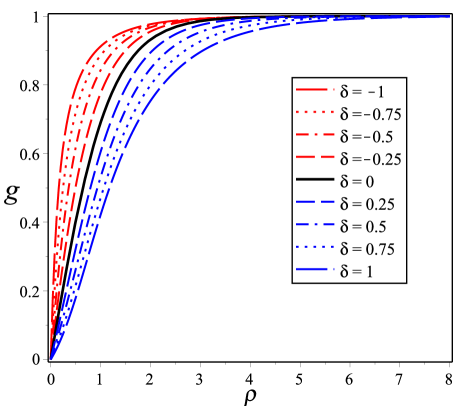
Figure 1: The Higgs field profile ${g}(\rho)$ for $n=1$. The red lines represent the solutions for $\delta<0$, the black line ($\delta=0$) gives the BPS solution for the MH model, and the blue lines for $\delta>0$.

​

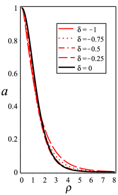
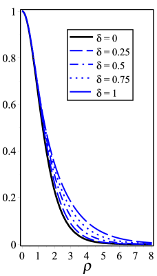
Figure 2: The gauge field profile ${a}(\rho)$ for $n=1$. The red lines represent the solutions for $\delta<0$, the black line ($\delta=0$) gives the BPS solution for the MH model, and the blue lines for $\delta>0$.

The left-side of Fig. 2 shows the gauge field profiles $a(\rho)$ for $n=1$ and $\delta<0$, which near the origin become slightly narrower than the MH ones ($\delta=0$). The right-side of Fig. 2 shows the profiles for $\delta>0$. In this case, near the origin they are almost overlapped to the ones of the MH model. We observe that for $\delta\neq 0$, at some distance from the origin, the profiles become wider than the MH one. This effect is minor for $\delta<0$ and major for $\delta>0$. This deviation augments with increasing $\left|\delta\right|$ values.

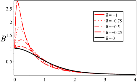
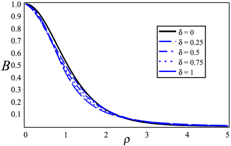
Figure 3: The magnetic field profile $B(\rho)$ for $n=1$. The red lines represent the solutions for $\delta<0$, the black line ($\delta=0$) gives the BPS solution for the MH model, and the blue line for $\delta>0$.

Upper Fig. 3 shows the magnetic field profiles, $B(\rho)$, for $n=1$ and $\delta<0$. At the origin, the magnetic field presents a finite value, $ev^{2},$ as the MH one. Close to the origin the LV parameter plays great influence, yielding a peak amplitude that forms a ring-like shaped structure. For more negative values of $\delta$, the peak is higher and more localized, while it becomes lower and wider as $\left|\delta\right|$ diminishes. Far from the origin, the magnetic field decays as much as the MH solution. This ring-like behavior, obtained for $n=1$, differs greatly from the lump-like MH ones, resembling the profiles of the Chern–Simons–Higgs models. Lower Fig. 3 shows the magnetic field profiles for $\delta>0$, which are very similar lumps to the MH ones, with the same value $ev^{2}$ at the origin. As one moves from the origin, the amplitude of $B(\rho)$ becomes slightly lesser than the MH one, yielding a little more localized defect.

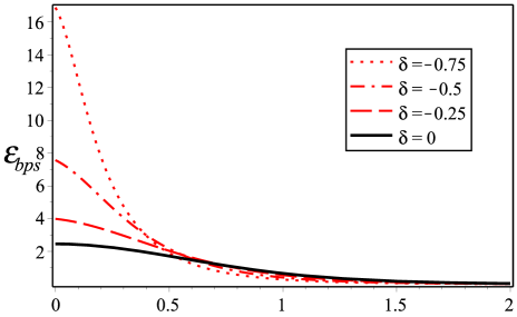
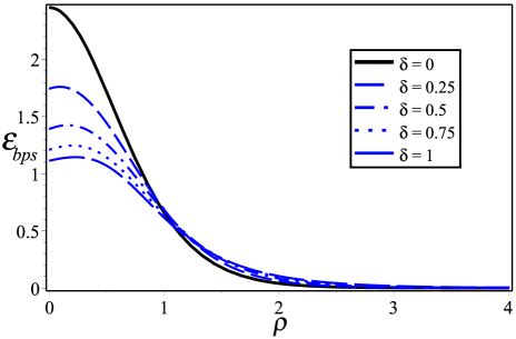
Figure 4: The BPS energy density profile $\varepsilon_{bps}(\rho)$ for $n=1$. The red lines represent the solutions for $\delta<0$, the black line ($\delta=0$) gives the BPS solution for the MH model, and the blue lines for $\delta>0$.

Fig. 4 shows the profiles of the BPS energy density $\varepsilon_{bps}$ for $n=1$. For $\delta<0$, we observe that the $\varepsilon_{bps}$ profiles present a lump shape similarly to the MH one, with a more pronounced and localized peak near to the origin. The peak amplitude and localization increase when $\delta$ becomes more negative. On the other hand, for $\delta>0$ (lower figure), the profiles maintain the lump-like shape, with the peak amplitude becoming smaller and less localized than the MH one. The peaks move away from the origin as $\delta$ increases. Numerically it is observed that for very large positive values of $\delta$, the BPS energy density amplitude at the origin has its lower bound at the value $e^{2}v^{4}$.

IV.2.2 Numerical solutions for $\delta=-0.75,0,0.75$ and $n=1,2,4,6,10,20$

Figs. 5 and 6 show the behavior of Higgs and gauge field profiles for various $n$ values with $\delta$ negative, null and positive. In both cases, the profiles become wider with raising $n$ values, but maintain a behavior similar to the case $n=1$ exhibited in Figs. 1 and 2, respectively.

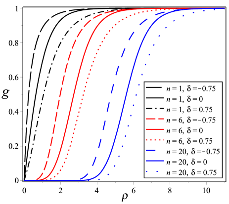
Figure 5: The Higgs field profiles $g(\rho)$ for $n=1,6,20$ and $\delta=-0.75,0,0.75$. The solid lines, $\delta=0$, represent the BPS solutions for the MH model.

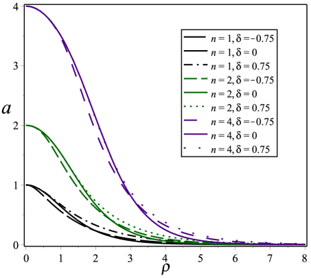
Figure 6: The gauge field profiles $a(\rho)$ for $n=1,2,4$ and $\delta=-0.75,0,0.75$. The solid lines, $\delta=0$, represent the BPS solutions for the MH model.

Fig. 7 depicts the magnetic field profiles for some values of $n$ and $\delta$. The upper figure provides the profiles for a negative value of $\delta$ ($\delta=-0.75$). It is observed the presence of peaks, corresponding to a ring-like behavior, which are more accentuated and closer to the origin for small winding number values. For large values of $n$, the ring structures have maximum amplitudes progressively smaller and located at an increasing distance from the origin. This behavior contrasts with the Maxwell–Higgs one, where the magnetic field profile displays a plateau whose width increases for larger $n$ values. So, the nonminimal coupling induces a ring-like behavior for the Abelian Higgs vortices when the LV parameter ($\delta$) takes negative values. The lower figure represents the magnetic field for a positive value of $\delta$ ($\delta=0.75$). It is observed that, for all values of $n$, the profiles follow closely the Maxwell–Higgs magnetic field behavior, presenting only a tiny deviation.

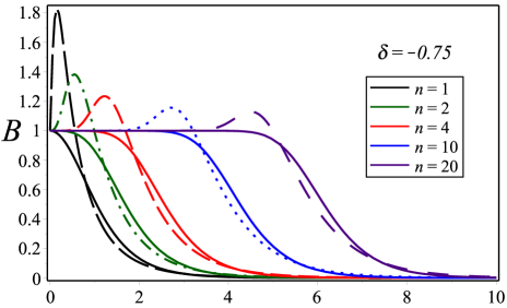
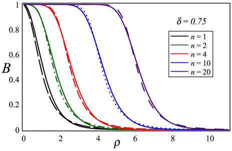
Figure 7: The magnetic field profiles $B(\rho)$ for $\delta=-0.75$ (upper figure) and $\delta=0.75$ (lower figure). In both cases, $n=1,2,4,10,20$. The solid lines represent the BPS solutions for the MH model.

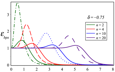
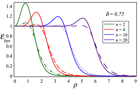
Figure 8: BPS energy density profiles $\varepsilon_{bps}(\rho)$ for $\delta=-0.75$ (upper figure) and $\delta=0.75$ (lower figure). In both cases, $n=2,4,10,20$. The solid lines represent the BPS solutions for the MH model.

Fig. 8 depicts the BPS energy density profiles for some values of $n\geq 2$ and fixed $\delta$. Despite the presence of the Lorentz violation, the profiles also display the ring-like behavior, as those of the MH model. In the upper picture, a negative LV parameter value ($\delta=-0.75$) enhances the amplitude peak of the ring shaped profiles, which become progressively lower for larger values of the winding number $n$. On the other side, in the lower figure, one notices that a positive LV parameter ($\delta=0.75)$ plays an opposite effect on the solutions, turning the peak amplitude much lesser than the MH ones. Consequently, for sufficiently large values of $n$, the Lorentz violation makes disappear the ring-like structure, reducing it to a simple plateau whose width increases with raising $n$ values.

V Remarks and conclusions

We have shown the existence of topological BPS or self-dual solutions in a MH model endowed with a CPT-odd and Lorentz-violating nonminimal coupling between the gauge and the Higgs fields. The Lorentz violation modifies self-dual or BPS equations of the MH model. Specifically, the Lorentz violation changes the usual symmetry breaking $|\phi|^{4}$-potential by introducing a new derivative self-interaction whose coupling constant is the own LV vector background. The present CPT-odd self-dual configurations are now electrically neutral in contraposition to the CPT-odd charged cases in which the Lorentz violation is included in the kinetic sector Lazar ; Alyson ; claudio2 . Another feature of this nonminimal model is that the Higgs field and magnetic field solutions for $-\xi_{j}$ are different from the ones for $\xi_{j}$.

We have solved the BPS equation for axially symmetric vortex solutions. Besides the control on the width of the vortex core, the magnetic field profiles undergo relevant modifications for negative values of the LV parameter, inducing a ring-like behavior similar to one appearing in Abelian Higgs models containing the Chern–Simons term. The BPS energy density also suffers significant deviations from the MH profiles for all values of the LV parameter, being observed that, for $n\geq 2$, the ring-like behavior can be enhanced (becoming much closer to the MCSH behavior) for a positive LV parameter or strongly attenuated (in relation to the MH typical profiles) for negative values of LV parameter. We have thus argued that the consideration of a preferred direction in spacetime, by means of a nonminimal coupling, is a factor that can indeed enrich the description of vortex structures.

- (1) A. A. Abrikosov, Zh. Eksp. Teor. Fiz. 32, 1442 (1957); Sov. Phys. - JETP 5, 1174 (1957); J. Phys. Chem. Solid. 2, 199 (1957).
- (2) V. L. Ginzburg and L. D. Landau, JETP 20, 1064 (1950).
- (3) L. Onsager, Nuovo Cimento 9, 6, 279 (1949); R. P. Feyn- man, in Chapter II Application of Quantum Mechanics to Liquid Helium, Progress in Low Temperature Physics, Vol. 1, edited by C. Gorte (Elsevier, 1955) pp. 1753.
- (4) H. Nielsen and P. Olesen, Nucl. Phys. B 61, 45 (1973).
- (5) F. A. Schaposnik and H. J. de Vega, Phys. Rev. D 14, 1100 (1976).
- (6) S. Hyun, J. Shin, J. H. Yee, and H.-j. Lee, Phys. Rev. D 55, 3900 (1997).
- (7) H. J. de Vega and F. A. Schaposnik, Phys. Rev. Lett. 56, 2564 (1986); S. K. Paul and A. Khare, Phys. Lett. B 174, 420 (1986).
- (8) J. Hong, Y. Kim, and P. Y. Pac, Phys. Rev. Lett. 64, 2230 (1990); R. Jackiw and E. J. Weinberg, 64, 2234 (1990); R. Jackiw, K. Lee, and E. J. Weinberg, Phys. Rev. D 42, 3488 (1990); A. Khare, Phys. Lett. B 255, 393 (1991); Proc. Indian Natn. Sci. Acad. A 61, 161 (1995).
- (9) M. K. Prasad and C. M. Sommerfeld, Phys. Rev. Lett. 35, 760 (1975); E. B. Bogomol’nyi, Yad. Fiz. 24, 861 (1976); Sov. J. Nucl. Phys. 24, 449 (1976).
- (10) D. Colladay and V. A. Kostelecký, Phys. Rev. D 55, 6760 (1997); 58, 116002 (1998); S. Coleman and S. L. Glashow, 59, 116008 (1999).
- (11) V. A. Kostelecký and S. Samuel, Phys. Rev. Lett. 63, 224 (1989); Phys. Rev. D 40, 1886 (1989); 39, 683 (1989); Phys. Rev. Lett. 66, 1811 (1991); V. A. Kostelecký and R. Potting, Phys. Rev. D 51, 3923 (1995).
- (12) M. N. Barreto, D. Bazeia, and R. Menezes, Phys. Rev. D 73, 065015 (2006).
- (13) A. de Souza Dutra, M. Hott, and F. A. Barone, Phys. Rev. D 74, 085030(2006).
- (14) D. Bazeia, M. M. Ferreira. Jr., A. Gomes, and R. Menezes, Physica D: Nonlinear Phenomena 239, 942 (2010).
- (15) A. de Souza Dutra and R. A. C. Correa, Phys. Rev. D 83, 105007 (2011).
- (16) M. D. Seifert, Phys. Rev. Lett. 105, 201601 (2010); Phys. Rev. D 82, 125015 (2010).
- (17) A. P. Baêta Scarpelli, H. Belich, J. L. Boldo, and J. A. Helayël-Neto, Phys. Rev. D 67, 085021 (2003).
- (18) R. Casana, G. Lazar, Phys. Rev. D 90, 065007 (2014).
- (19) C. Miller, R. Casana, M. M. Ferreira Jr., and E. da Hora, Phys. Rev. D 86, 065011 (2012).
- (20) R. Casana, M. M. Ferreira Jr., E. da Hora, and C. Miller, Phys. Lett. B 718, 620 (2012).
- (21) C.H. Coronado Villalobos, J.M. Hoff da Silva, M.B. Hott, H. Belich, Eur. Phys. J. C 74, 27991 (2014).
- (22) H. Belich, F.J.L. Leal, H.L.C. Louzada, M.T.D. Orlando, Phys.Rev. D 86, 125037 (2012).
- (23) L. Sourrouille, Phys. Rev. D 89, 087702 (2014).
- (24) R. Casana and L. Sourrouille, Phys. Lett. B 726, 488 (2013).
- (25) R. Casana, M. M. Ferreira Jr., E. da Hora, A. B. F. Neves, Eur. Phys. J. C74, 3064 (2014).
- (26) A. de Souza Dutra, R. A. C. Correa, Adv. High Energy Phys. 2015, 673716 (2015).
- (27) R. A. C. Correa, R. da Rocha, A. de Souza Dutra, Ann. Phys. 359, 198 (2015).
- (28) R. A. C. Correa, Roldao da Rocha, A. de Souza Dutra, Phys. Rev. D 91, 125021 (2015).
- (29) M. Torres, Phys. Rev. D 46, 2295 (1992); J. Escalona, M. Torres, and A. Antillón, Mod. Phys. Lett. A 08, 2955 (1993).
- (30) P. K. Ghosh, Phys. Rev. D 49, 5458 (1994).
- (31) T. Lee and H. Min, Phys. Rev. D 50, 7738 (1994); M. Torres, Rev. D 51, 4533 (1995); A. Antillón, J. Escalona, and M. Torres, Phys. Rev. D 55, 6327 (1997); F. Chandelier, Y. Georgelin, M. Lassaut, T. Masson, and J.C.Wallet, Phys. Rev. D 70, 065016 (2004).
- (32) L. H. C. Borges, A. G. Dias, A. F. Ferrari, J. R. Nascimento, A. Yu. Petrov, Phys. Rev. D 89, 045005 (2014).
- (33) L. H. C. Borges, A. G. Dias, A. F. Ferrari, J. R. Nascimento, A. Yu. Petrov, Phys. Lett. B 756, 332 (2016).
- (34) V.A. Kostelecky and M. Mewes, Phys. Rev. 80, 015020 (2009); M. Schreck, Phys. Rev. 89, 105019 (2014); M. Cambiaso, R. Lehnert, R. Potting, Phys. Rev. D 85, 085023 (2012); M. Schreck, Phys. Rev. D 89, 105019 (2014) ; Phys. Rev. D 90, 085025 (2014); B. Agostini, F. A. Barone, F. E. Barone, P. Gaete, J. A. Helayël-Neto, Phys. Lett. B 708, 212 (2012); L. Campanelli, Phys. Rev. D 90, 105014 (2014); R. Bufalo, B.M. Pimentel, D.E. Soto, Physical Review D 90, 085012 (2014).
- (35) V.A. Kostelecky and M. Mewes, Phys. Rev. 88, 096006 (2013); M. Schreck, Phys. Rev. 90, 085025 (2014).
- (36) H. Belich, T. Costa-Soares, M. M. Ferreira, Jr., and J. A. Helayël-Neto, Eur. Phys. J. C 41, 421 (2005).
- (37) B. Charneski, M. Gomes, R.V. Maluf, and A. J. da Silva, Phys. Rev. D 86, 045003 (2012).
- (38) T. Mariz, J. R. Nascimento, A.Y. Petrov, Phys. Rev. D 85, 125003 (2012); G. Gazzola, H. G. Fargnoli, A. P. Baêta Scarpelli, Marcos Sampaio, M. C. Nemes, J. Phys. G 39, 035002 (2012); A. P. Baeta Scarpelli, J. Phys. G 39, 125001 (2012); L. C. T. Brito, H. G. Fargnoli, and A. P. Baeta Scarpelli, Phys. Rev. D 87, 125023 (2013).
- (39) K. Bakke and H. Belich, J. Phys. G 39, 085001 (2012); K.Bakke, H. Belich, and E. O. Silva, J. Math. Phys. (N.Y.) 52, 063505 (2011); J. Phys. G 39, 055004 (2012); Ann. Phys. (Berlin) 523, 910 (2011); K. Bakke and H. Belich, Eur. Phys. J. Plus 127, 102 (2012).
- (40) H. Belich, E. O. Silva, M. M. Ferreira, Jr., and M. T. D. Orlando, Phys. Rev. D 83, 125025 (2011).
- (41) R. Casana, C. F. Farias, and M. M. Ferreira, Jr., Phys. Rev. D 92, 125024 (2015).
- (42) R. Casana, C. F. Farias, M. M. Ferreira Jr., and G. Lazar, Phys. Rev. D 94, 065036 (2016).