Thermal shape fluctuation model study of the giant dipole resonance in ¹⁵²Gd

Abstract

We have studied the giant dipole resonance (GDR) in the hot and rotating nucleus ¹⁵²Gd within the framework of thermal shape fluctuation model (TSFM) built on the microscopic-macroscopic calculations of the free energies with a macroscopic approach for the GDR. Our results for GDR cross sections are in good agreement with the experimental values except for a component peaking around 17 MeV where the data has large uncertainties. Such a component is beyond our description which properly takes care of the splitting of GDR components due to the deformation and Coriolis effects. Around this 17 MeV lies the half maximum in experimental cross sections, and hence the extracted GDR widths and deformations (estimated from these widths) turn out to be overestimated and less reliable. Reproducing these widths with empirical formulae could conceal the information contained in the cross sections. Fully microscopic GDR calculations and a more careful look at the data could be useful to understand the GDR component around 17 MeV. We also discuss the occurrence of $\gamma$-softness in the free energy surfaces of ¹⁵²Gd and its role on GDR.

I Introduction

In a simplistic view, the giant dipole resonance (GDR) is due to collective oscillations between protons and neutrons under the influence of the electromagnetic field induced by the emitted/absorbed photons, which results in a large peak in the emission/absorption spectrum of $\gamma$-rays. This fundamental mode of nuclear collective excitation can be built on any state and hence GDR can probe the structure of the nucleus even at finite temperature ($T$) and angular momentum ($I$) Alhassid (1999); Snover (1986); Gaardhøje (1992).

In a macroscopic theoretical description of GDR, the GDR observables are coupled with the shape degrees of freedom. Since the nucleus is a tiny system, the thermal fluctuations are more dominant. In the thermal shape fluctuation model (TSFM), the GDR observables are obtained as the average over all the possible shapes of the nucleus Alhassid (1999); Alhassid and Bush (1989); Arumugam et al. (2004). In most of such models, the probability of finding the nucleus with a given shape is given in terms of the free energy calculated in a microscopic-macroscopic approach.

In a microscopic way, the GDR can be explained in terms of particle-hole, particle-particle and hole-hole excitations Gaardhøje (1992). One such approach is the phonon damping model which has been proved to be quite successful in explaining the measured GDR widths ($\Gamma$) as a function of $T$ Dang et al. (1998); Dang and Arima (1998); Dang et al. (1999). Recently, these calculations are extended to include the angular momentum for non-collective rotations Dang et al. (2013). In another microscopic approach, the GDR in hot and rotating nuclei were studied within the frame work of linear response theory along with static path approximation to the grand canonical partition function Ansari et al. (2000, 2001). Most of the other microscopic approaches for GDR Daoutidis and Ring (2011); Lyutorovich et al. (2012); Bacca et al. (2013) are not extended to hot and rotating nuclei.

Apart from the theoretical models, phenomenological formulae were also introduced to explain the global properties of $\Gamma$ Kusnezov et al. (1998); Pandit et al. (2012) in hot and rotating nuclei. These formulae are constructed to fit the experimental $\Gamma$. The results of these phenomenological formulae are similar to those of the TSFM in some cases.

Despite a number of experiments been carried out to understand the properties of GDR and the effect of $T$ and $I$ on GDR Chakrabarty et al. (2006); Mukul et al. (2014, 2013), still there are several open questions. By large, the measured $\Gamma$ are well interpreted by TSFM calculations, and the phenomenological scaling formula (PSF) Kusnezov et al. (1998) description also was successful in many cases. The failure of PSF and TSFM at low-$T$ is recently analyzed Pandit et al. (2012) and the PSF is modified suitably, leading to a critical temperature formula (CTF) which overcomes the discrepancies at low-$T$. The microscopic origin of such discrepancy is quite known Dang et al. (2000) to be due to pairing and extension of the TSFM to include pairing proved that TSFM is quite successful at low-$T$ also Rhine Kumar et al. (2015, 2014). Another case where the PSF was observed to be insufficient to explain the measured $\Gamma$ is the hot and rotating nucleus ¹⁵²Gd. It is shown in Ref. Chakrabarty et al. (2010) that the PSF could not explain the $\Gamma$ measured at two excitation energies with a single value for the parameter of the PSF (reduced width, $\Gamma_{0}$). This work highlighted the need for performing proper TSFM calculations specifically for this system to understand the GDR properties. The CTF was demonstrated Pandit et al. (2013a) to be successful and the discrepancy with the PSF was attributed to the role of GDR induced quadrupole moment Simenel and Chomaz (2009, 2003). This argument was generalized to TSFM based on the fact that the PSF mostly mimics the results of TSFM. Simpler TSFM calculations with the liquid drop model (LDM) were reported in Ref. Pandit et al. (2013b) where the average deformation ($\langle\beta\rangle)$ of ¹⁵²Gd (and other selected nuclei) extracted from the measured $\Gamma$ were shown to be compatible with the results of LDM and CTF.

In this article we present our results from the TSFM calculations and analyze the structure of the hot and rotating ¹⁵²Gd. We employ the TSFM built on Nilsson-Strutinsky (NS) calculations with a macroscopic approach to GDR. Our formalism is well tested to explain several GDR observations at higher $T$ and $I$ Arumugam et al. (2004); Arumugam et al. (2005a, b, c). In a recent work Mukul et al. (2014, 2013), the GDR properties of hot and rotating ¹⁴⁴Sm were studied and the experimental data were very well explained with the TSFM results. A short description about this formalism and our results for the hot and rotating nucleus ¹⁵²Gd, are discussed in the forthcoming sections.

II Theoretical Framework

Within the TSFM, the expectation value of an observable $\mathcal{O}$ incorporating both thermal fluctuations and orientation fluctuations is given by Alhassid and Bush (1991); Alhassid (1999)

$$\langle\mathcal{O}\rangle_{\beta,\gamma,\theta,\phi}=\frac{\int_{\beta}\int_{\gamma}\int_{\theta}\int_{\phi}\mathcal{D}[\alpha]\exp\left[{-F_{\mathrm{TOT}}(T,I;\beta,\gamma,\theta,\phi)/T}\right]\Im_{\mathrm{TOT}}^{-3/2}\mathcal{O}}{\int_{\beta}\int_{\gamma}\int_{\theta}\int_{\phi}\mathcal{D}[\alpha]\exp\left[{-F_{\mathrm{TOT}}(T,I;\beta,\gamma,\theta,\phi)/T}\right]\Im_{\mathrm{TOT}}^{-3/2}}\;$$ (1)

where $\phi,\theta$ are the Euler angles specifying the intrinsic orientation of the nucleus with respect to the axis of rotation. $\beta$ and $\gamma$ are the deformation parameters describing the quadrupole shapes. The volume element is chosen to be $\mathcal{D}[\alpha]=\beta^{4}|\sin 3\gamma|\,d\beta\,d\gamma\,\sin\theta\,d\theta\,d\phi$. $\Im_{\mathrm{TOT}}=\Im_{rig}+\delta\Im$, where $\Im_{rig}=\Im_{x^{\prime}x^{\prime}}\cos^{2}\phi\ \sin^{2}\theta+\Im_{y^{\prime}y^{\prime}}\sin^{2}\phi\ \sin^{2}\theta+\Im_{z^{\prime}z^{\prime}}\cos^{2}\theta$, is the moment of inertia, about an axis with the orientation $\theta$ and $\phi$, given in terms of the principal moments of inertia $\Im_{x^{\prime}x^{\prime}},\ \Im_{y^{\prime}y^{\prime}},\ \Im_{z^{\prime}z^{\prime}}$. $\delta\Im$ is the shell correction for moment of inertia. The total free energy ($F_{\mathrm{TOT}}$) at a fixed deformation is calculated using the Nilsson-Strutinsky method extended to high spin and temperature Arumugam et al. (2004); Arumugam et al. (2005a).

$$F_{\mathrm{TOT}}=E_{\mathrm{LDM}}+\sum_{p,n}\delta F^{\omega}+\frac{1}{2}\omega({I_{\mathrm{TOT}}+\sum_{p,n}\delta I)}\;,$$ (2)

where $E_{\mathrm{LDM}}$ is the liquid-drop energy and $\delta F^{\omega}=F^{\omega}-\widetilde{F}^{\omega}$ is the shell correction. $\omega$ and $I_{\mathrm{TOT}}$ are the angular velocity and the total spin, respectively. $\delta I$ is the shell correction to the spin. The microscopic free energy can be calculated using the expression Arumugam et al. (2005a)

$$F^{\omega}=\sum_{i=1}^{\infty}e_{i}^{\omega}n_{i}-T\sum_{i=1}^{\infty}s_{i}\;.$$ (3)

The single-particle energies ($e_{i}^{\omega}$) are obtained by diagonalizing the triaxial Nilsson Hamiltonian in a cylindrical representation up to first twelve major shells. $n_{i}$ are the occupation numbers given by

$$n_{i}=\frac{1}{1+\exp\left(\frac{e_{i}^{\omega}-\lambda}{T}\right)}$$ (4)

where $\lambda$ is the chemical potential obtained using the constraint $\sum_{i=1}^{\infty}n_{i}=N_{p}$ and $N_{p}$ is the total number of particles. $s_{i}$ are the single-particle entropies and the total entropy $S=\sum_{i=1}^{\infty}s_{i}$ can be written as

$$S=-\sum_{i=1}^{\infty}\left[n_{i}\ln n_{i}+(1-n_{i})\ln(1-n_{i})\right]\;.$$ (5)

$\widetilde{F}^{\omega}$ is calculated in a Strutinsky way Strutinsky (1967) with exact $T$ and $I$ dependance and more details in this regard can be found in Refs. Arumugam et al. (2004); Arumugam et al. (2005a). The effect of orientation fluctuations is negligible while calculating the observables like GDR cross sections and the width Ormand et al. (1997); Ansari et al. (2001); Arumugam et al. (2004); Arumugam et al. (2005a), and hence we have neglected the orientation fluctuations in the present calculations.

The nuclear shapes are related to the GDR observables using a macroscopic model Hilton (1983); Arumugam et al. (2004); Shanmugam and Thiagasundaram (1988) comprising an anisotropic harmonic oscillator potential with a separable dipole-dipole interaction. The Hamiltonian describing GDR excitations can be written as

$$H=H_{osc}+\eta\ D^{\dagger}D\;.$$ (6)

Here $H_{osc}$ stands for the anisotropic harmonic oscillator Hamiltonian, $\eta$ and $D$ represent the dipole-dipole interaction strength and dipole operator, respectively. The total GDR cross section ($\sigma$) is constructed by summing the individual Lorentzians with the peaks at the GDR energies ($E_{i}$) given by the frequencies corresponding to $H$. The width of these individual components depend on $E_{i}$ through the relation Carlos et al. (1974)

$$\Gamma_{i}\approx 0.026E_{i}^{1.9}\;.$$ (7)

The GDR full width at half maximum, comparable with the measured value, is determined from the total GDR cross section, $\sigma$ averaged over all the possible shapes.

III Results and discussion

The GDR cross sections and GDR width for the nucleus ¹⁵²Gd are reported in Ref. Chakrabarty et al. (2006) for the beam energy, $E\sim 149$ MeV and later compiled along with the data at $E\sim 185$ MeV in the Ref. Chakrabarty et al. (2010). TSFM calculations with free energies from LDM were reported in Ref. Pandit et al. (2013b). We start our analysis by comparing the GDR cross sections calculated with TSFM, and the experimental cross sections at beam energy, $E\sim 149$ MeV. These results are presented in Fig. 1. The TSFM calculations are carried out with two different values for the dipole-dipole interaction parameter $\eta$. The value of $\eta$ as $2.3$ is chosen by fitting the experimental cross sections. In this case, we have a good agreement between the experimental and theoretical GDR cross sections represented by the solid lines. However, as shown in Table 1, the corresponding TSFM GDR widths ($\Gamma_{\mathrm{TSFM}}$) are smaller than the experimental GDR widths ($\Gamma_{\mathrm{Expt}}$). On a careful examination of the cross sections, shown in Fig. 1, we can note that the experimental data in the higher energy side around the half maximum is quite scattered in most of the cases. Due to this scattered data, the fitting of smooth curves (two component Lorentzian) will carry large errors as reported in Ref. Chakrabarty et al. (2010). These experimental cross sections, with large errors in the higher energies, tend to yield an overestimated width.

A perfect fit to the GDR cross sections could be possible with a fragmented GDR spectrum. In a microscopic approach, there can be numerous components of GDR corresponding to various combinations of particle-hole ($ph$), particle-particle ($pp$), and hole-hole ($hh$) excitations Goeke and Speth (1982). The strength functions for these components can be calculated microscopically but the width is rather artificially introduced. For example, in Ref. Dang et al. (1999) one can see a fragmented GDR for ¹²⁰Sn (Fig. 3 of Ref. Dang et al. (1999)) with a protruding component around $20$ MeV. Restricting the coupling to $ph$, $pp$, and $hh$ configurations via the doorways can lead to a different scenario (Fig. 5 of Ref. Dang et al. (1999)). These variations can be understood in terms of the choice of doorway configurations but it is rather difficult to associate a simple physical process. In a macroscopic approach, the picture of splitting of GDR components is quite vivid in terms of the deformation and the Coriolis effects leading to a maximum of five components Hilton (1983). Even after considering all these effects, our model does not yield such a fragmented GDR consistent with the experimental data. The temperatures corresponding to the observations are sufficiently high so that the macroscopic approach is good enough. The fit achieved for cross sections by our calculations are quite reasonable considering the uncertainties in the data. Hence, the discrepancy in matching the width as shown in Table 1, shall be attributed to the inaccuracy in experimental cross sections. In other words, with large uncertainties in cross sections, it could be inappropriate to rely on $\Gamma_{\mathrm{Expt}}$ for comparison with the theory. This fact is exemplified by our calculations with $\eta=3.35$ which fits the $\Gamma_{\mathrm{Expt}}$ in a better way as shown in the last column of Table 1. This choice of $\eta$ is far from the systematic values Arumugam et al. (2004) and yields the cross sections which are very far from the experimental data as shown in Fig. 1. with dashed lines.

Figure 1: The GDR experimental cross sections (filled circles) of ¹⁵²Gd at beam energy $E\sim 149$ MeV taken from Ref. Chakrabarty et al. (2010), are compared with the TSFM results obtained using $\eta=2.3$ (solid lines) and $\eta=3.35$ (dashed lines) at different values of temperature ($T$) and angular momentum ($I$).

Table 1: The experimental GDR widths ($\Gamma_{\mathrm{Expt}}$) in ¹⁵²Gd at beam energy $E\sim 149$ MeV are compared with the GDR widths calculated with TSFM ($\Gamma_{\mathrm{TSFM}}$) using two different values for the dipole-dipole interaction strength parameter $\eta$. The temperature ($T$) and angular momentum ($I$) correspond to the average values extracted from experimental data Chakrabarty et al. (2010).

$T$	$I$	$\Gamma_{\mathrm{Expt}}$	$\Gamma_{\mathrm{TSFM}}$(MeV)
(MeV)	$(\hbar)$	(MeV )	$\eta=2.3$	$\eta=3.35$
1.59	27.0	8.5$\pm$0.3	7.4	8.7
1.56	32.1	8.5$\pm$0.3	7.5	8.8
1.53	37.3	8.8$\pm$0.4	7.7	9.0
1.47	44.0	8.8$\pm$0.4	8.0	9.2
1.39	50.9	8.8$\pm$0.4	8.4	9.6
1.34	55.1	10.1$\pm$0.5	8.7	9.8

Figure 2: Similar to Fig. 1 but at beam energy $E\sim 185$ MeV.

Table 2: Similar to Table 1 but at beam energy $E\sim 185$ MeV.

$T$	$I$	$\Gamma_{\mathrm{Expt}}$	$\Gamma_{\mathrm{TSFM}}$(MeV)
(MeV)	$(\hbar)$	(MeV)	$\eta=2.3$	$\eta=3.35$
1.91	13.3	9.5$\pm$0.5	7.4	8.7
1.87	22.9	9.8$\pm$0.3	7.5	8.8
1.81	34.5	10.0$\pm$0.4	7.9	9.2
1.75	43.7	10.9$\pm$0.5	8.3	9.6
1.69	51.2	11.1$\pm$0.4	8.7	9.9
1.64	56.5	11.7$\pm$0.8	9.1	10.4

Our results for cross sections at beam energy, $E\sim 185$ MeV are presented in Fig. 2, in comparison with the experimental data. In this case also the quality of agreement between our calculations and the data is good except for the very high angular momenta. The corresponding widths are presented in Table 2. From these results at $E\sim 185$ MeV, we see the same trend as noticed in the case of $E\sim 149$ MeV, viz., (i) the cross sections around the half maximum at the higher energy are scattered leading to overestimation of $\Gamma_{\mathrm{Expt}}$, and (ii) with larger $\eta$, we can obtain a better fit to $\Gamma_{\mathrm{Expt}}$ but the corresponding theoretical cross sections are far from the data. In the present case, the hump at high energy is more pronounced and renders larger width. A simple double Lorentzian fit would suggest a second peak around 15 MeV which is perhaps inexplicable within the present theoretical approach. These facts strengthen our argument that one should not rely on the GDR width, when the cross sections have large uncertainties.

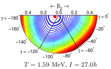
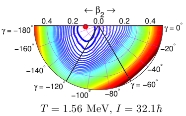
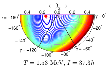
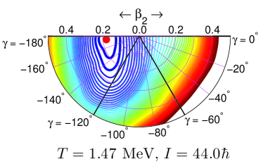
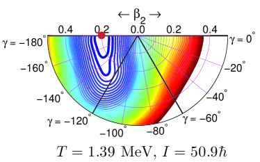
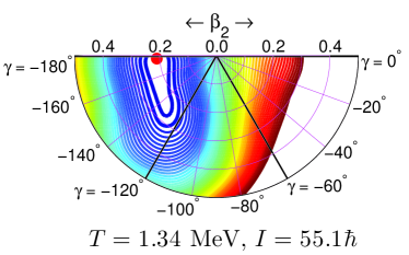
         (a)                                                             (b)          (c)                                                             (d)          (e)                                                             (f)

Figure 3: (Color online) The free energy surfaces (FES) of ¹⁵²Gd at different temperature ($T$) and angular momentum ($I$) combinations corresponding to the data measured at beam energy $E\sim 149$ MeV. In this convention, $\gamma=0^{\circ}$ and $-120^{\circ}$ represent the non-collective and collective prolate shapes, respectively; $\gamma=-180^{\circ}$ and $-60^{\circ}$ represent the non-collective and collective oblate shapes, respectively. The contour line spacing is 0.2 MeV. The most probable shape is represented by a filled circle and first two minima are represented by thick lines.

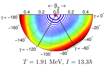
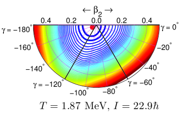
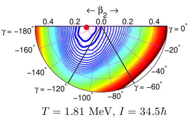
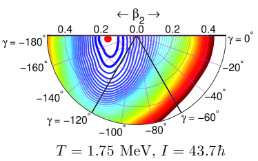
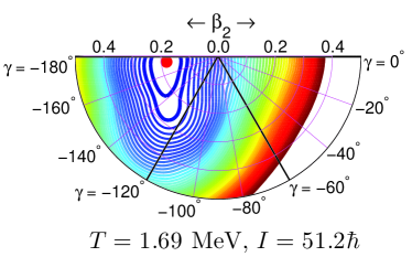
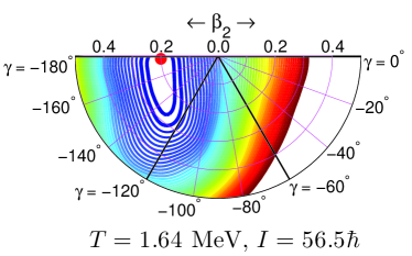
         (a)                                                             (b)          (c)                                                             (d)          (e)                                                             (f)

Figure 4: (Color online) Similar to Fig. 3 but for beam energy, $E\sim 185$ MeV.

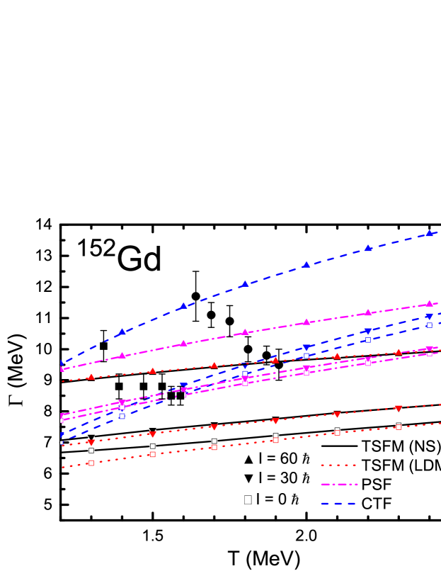
Figure 5: (Color online) The GDR width ($\Gamma$) in ¹⁵²Gd calculated with various approaches at different angular momenta are plotted as a function of temperature ($T$). The phenomenological scaling formula (PSF) Kusnezov et al. (1998), critical temperature formula (CTF) Pandit et al. (2012), TSFM (LDM), and TSFM (NS) results are represented by dash-dotted, dashed, dotted and solid lines, respectively. The $I=0\hbar,30\hbar$ and $60\hbar$ are represented by open squares, downward triangles, and upward triangles, respectively. The experimental results are taken for Ref. Chakrabarty et al. (2010), the results at beam energy $E\sim 149$ MeV and $185$ MeV are represented by filled squares, and filled circles, respectively.

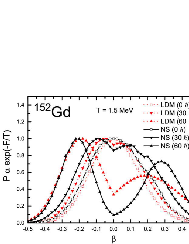
Figure 6: (Color online) The probability distribution of ¹⁵²Gd shapes calculated with liquid drop model (LDM) and Nilsson-Strutinsky (NS) approach, at different angular momenta ($I$) are plotted as a function of axial deformation parameter $\beta$. The peaks are normalized to unity. For the axially deformed shapes, the positive and negative values of $\beta$ can be associated to $\gamma=-180^{\circ}$ and $-120^{\circ}$, respectively. The LDM and NS results are represented by dotted and solid lines, respectively. The results for $I=0\hbar,30\hbar$ and $60\hbar$ are represented by squares, downward triangles, and upward triangles, respectively.

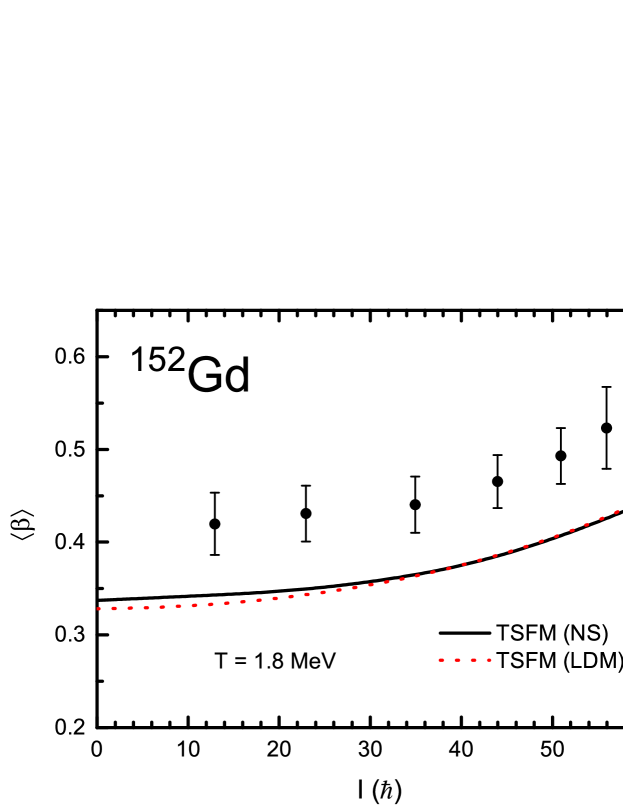
Figure 7: (Color online) The average deformation ($\langle\beta\rangle$) of ¹⁵²Gd calculated with liquid drop model (LDM) and Nilsson-Strutinsky (NS) approach, at temperature ($T=1.8$ MeV) is plotted as a function of angular momentum ($I$). The LDM and NS results are represented by dotted and solid lines, respectively. The values extracted from GDR data Pandit et al. (2013b) are represented by filled circles.

In order to understand the variation in GDR cross sections in terms of the shape transitions in the nucleus ¹⁵²Gd, we present the free energy surfaces (FES) calculated within our microscopic-macroscopic approach. These FES at different $T$ and $I$ combinations corresponding to $E\sim 149$ MeV are presented in Fig. 3. In general, it is well known that the GDR width ($\Gamma$) is proportional to the average axial deformation parameter $\beta$ ($\langle\beta\rangle$). Within our macroscopic model for GDR, for a given $\beta$, $\Gamma_{\text{Prolate}}>\Gamma_{\text{Triaxial}}>\Gamma_{\text{Oblate}}$. While considering thermal fluctuations, the shallowness of the minimum will lead to pronounced fluctuations and hence larger width. Apart from these shape effects, the GDR width increases with $I$ due to the Coriolis splitting and this change is rapid after $\sim 40\hbar$ in this mass region Kusnezov et al. (1998). From Fig. 3, we can note that at high-$T$ and low-$I$, the most probable shape is oblate with a small deformation. As $I$ increases, the most probable shape changes to a more deformed oblate. At high-$I$, the nucleus shows a clear $\gamma$-softness with the contour for $F\leq 0.4$ MeV being quite narrow with respect to $\beta$ ($\sim 0.2$) but spanning the region with $\gamma=-180^{\circ}$ to $-120^{\circ}$. In such a case, the GDR samples a wider variety of shapes and this sampling is enhanced by fluctuations at finite $T$. For a given $\beta$, since the oblate shape leads to the least $\Gamma$, the $\gamma$-softness leads to an enhanced $\Gamma$ in comparison with that of the oblate shape.

Before discussing in detail the role of $\gamma$-softness in $\Gamma$, we present in Fig. 4, the FES corresponding to the $T$ and $I$ combinations extracted from the data measured at $E\sim 185$ MeV. In this case, at low-$I$, the most probable shape is spherical; as the $I$ increases the most probable shape changes to an oblate; and at high-$I$, the nucleus shows a clear $\gamma$-softness similar to the previous case. An overall but important observation, from the two sets of FES, is that there are no drastic shape transitions as the $I$ increases. This observation implies that we do not expect any drastic change in the $\Gamma$ with the variation of $T$ and $I$, within the limits suggested by the data at both excitation energies. Secondly, some interesting features seen in the FES need not be reflected in the observables due to the thermal fluctuations which can play a strong role in the considered range of $T$ ($\sim 1.5$ MeV) by smearing out the structural changes caused by shell effects. Such smearing effects can be well depicted while comparing our results with those obtained using the liquid drop model (LDM) FES instead of the FES from the Nilsson-Strutinsky (NS) approach, as shown in Fig. 5, where the former and latter results are depicted by dotted and solid lines, respectively. Except for low-$T$ and low-$I$ the TSFM results with FES from LDM and NS, agree well. Thus a LDM description is quite reasonable for the GDR in ¹⁵²Gd. Consequently, we observe that some interesting shape effects like the $\gamma$-softness and the shape transitions, as depicted by the FES, are not effectively reflected in the corresponding $\Gamma$. This can be ascribed to the domination of thermal fluctuations which smear out the effects of shape transitions. To see this in detail, we have plotted in Fig. 6 the probabilities corresponding to different shapes as given by the Boltzmann’s factor [$\exp(-F/T)$] which can be understood as the weights corresponding to the shapes while averaging the cross sections over different shapes [Eq. (1)].

In Fig. 6, first we would like to draw attention towards the calculations at $0\hbar$ (open squares) where we can see that the probability distribution ($P$) is wider in the case of NS calculations and hence yield larger $\Gamma$ (as seen in Fig. 5). This difference between LDM and NS results is obviously due to shell effects which would melt as the temperature increases. This difference in $P$ seems to be more at 30$\hbar$ but the contribution from triaxial shapes become significant (not depicted in Fig. 6) due to the thermal fluctuations and hence the resulting $\Gamma$ are not very different. The dominance of thermal shape fluctuations is quite vivid in the case of $I=60\hbar,$ as evident from the very distinct $P$ for LDM and NS leading to same $\Gamma$. It would be interesting to see how well these shape effects can be reflected by $\Gamma$ at lower $T$ where the shape fluctuations are not that dominant.

The correlation between the shape parameter $\beta$ and $\Gamma$ are well known Gallardo et al. (1985). In Ref. Pandit et al. (2013b) an empirical correlation is proposed so that one can estimate an “experimental” deformation ($\beta_{\rm exp}$) from the measured values of $\Gamma$. This allows us to compare the theoretical (average) deformations ($\langle\beta\rangle$) with $\beta_{\rm exp}$ in a way independent of the model for the GDR. Such an analysis has been carried out in Ref. Pandit et al. (2013b) for the nuclei ⁵⁹Cu, ¹¹⁰Sn, ¹¹³Sb, ¹⁵²Gd, and ¹⁷⁶W. Our results for $\langle\beta\rangle$ in ¹⁵²Gd obtained with TSFM calculations are presented in Fig. 7. The TSFM results with LDM and NS methods are represented by dotted and solid lines, respectively and the $\beta_{\rm exp}$ taken from Ref. Pandit et al. (2013b) are represented by filled circles. We infer that our TSFM calculations underestimate the deformation and is explicable as discussed in the case of our results for $\Gamma$ shown in Fig. 5 and hence strengthen the associated arguments. Here such a discrepancy can be seen as a function of angular momentum ($I$). The $\langle\beta\rangle$ of ¹⁵²Gd obtained with the TSFM (LDM) presented in Fig. 3 of Ref. Pandit et al. (2013b) shows a higher value, when compared with our results. Such results based on LDM (at least for $I=0$) should vary smoothly with the mass number but an abrupt raise in $\langle\beta\rangle$ of ¹⁵²Gd could be seen in Fig. 3 of Ref. Pandit et al. (2013b). This raise could be possible with the choice of the parameters in the calculations which are not known clearly.

Apart from the TSFM results, in Fig. 5, we have presented the experimental $\Gamma$ along with the values calculated using the phenomenological scaling formula (PSF) Kusnezov et al. (1998) and the critical temperature formula (CTF) Pandit et al. (2012). In the PSF, the ground state GDR width is assumed to be $\Gamma_{0}=3.8$ MeV all the other parameters are fitted empirically in a global way. As shown in Ref. Pandit et al. (2013a), the CTF can explain the enhanced $\Gamma$ whereas the PSF fails in this regard. However, a larger $\Gamma_{0}$ of 5.7 MeV is used to reproduce the measured $\Gamma$. Another parameter of CTF is the critical temperature, $T_{c}$, which is also adjusted to get a better fit with the experimental results. Naturally, with the help of two adjustable parameters, the CTF could explain the data much better than the PSF. These parameters can change the rate at which $\Gamma$ changes with $I$ and $T$. At $T=1.2$ MeV, the difference in $\Gamma$ values with PSF (dash-dotted lines) at two extreme values of $I$ is, $\delta\Gamma\sim 1.6$ MeV. Whereas, with CTF (dashed lines), $\delta\Gamma\sim 2.5$ MeV. So the CTF parameters are chosen to have a stiff $\Gamma$ with respect to both $I$ and $T$, and hence the CTF is able to explain the $\Gamma_{\mathrm{Expt}}$ in a larger range. Results from such a stiff parameterization cover more regions in Fig. 5 and eventually the CTF encompasses all the experimental data. The success of CTF in explaining the $\Gamma$ in an empirical manner shall not be considered as a validation of the extracted $\Gamma$, as the reliable information lies within the GDR cross sections.

IV Summary

The thermal shape fluctuation model (TSFM) study, of the giant dipole resonance (GDR) in the hot and rotating nucleus ¹⁵²Gd, reveals that there are no major anomalies in the values measured at two excitation energies. The GDR cross sections calculated with standard parameters are in agreement with the experiment, except for a shoulder around 17 MeV where the uncertainties are large. The component of GDR leading to such a shoulder cannot be explained within a macroscopic approach for GDR where the splitting due to the deformation and Coriolis effects are properly taken care. It could be instructive to see whether such a high energy component can be explained with fully microscopic approaches for GDR. It will also be useful to have a careful introspection of the data to ascertain the shoulder around 17 MeV. Due to this shoulder, the corresponding GDR widths are overestimated and hence their comparison with calculated values does not convey the complete information. Tuning the phenomenological parameterizations to reproduce such widths conceal the interesting information contained in the cross sections. The free energy surfaces in ¹⁵²Gd calculated at higher angular momenta show a clear gamma softness which could have led to larger GDR widths. However, such shape aspects are smeared by the thermal fluctuations which are dominant in the considered temperatures. It would be interesting to see how such shape effects survive at lower temperatures.

References

- Alhassid (1999) Y. Alhassid, Nucl. Phys. A 649, 107c (1999).
- Snover (1986) K. A. Snover, Ann. Rev. Nucl. Part. Sci. 36, 545 (1986).
- Gaardhøje (1992) J. J. Gaardhøje, Ann. Rev. Nucl. Part. Sci. 42, 483 (1992).
- Alhassid and Bush (1989) Y. Alhassid and B. Bush, Phys. Rev. Lett. 63, 2452 (1989).
- Arumugam et al. (2004) P. Arumugam, G. Shanmugam, and S. K. Patra, Phys. Rev. C 69, 054313 (2004).
- Dang et al. (1998) N. D. Dang, K. Tanabe, and A. Arima, Phys. Lett. B 445, 1 (1998).
- Dang and Arima (1998) N. D. Dang and A. Arima, Nucl. Phys. A 636, 427 (1998).
- Dang et al. (1999) N. D. Dang, K. Tanabe, and A. Arima, Nucl. Phys. A 645, 536 (1999).
- Dang et al. (2013) N. D. Dang, M. Ciemala, M. Kmiecik, and A. Maj, Phys. Rev. C 87, 054313 (2013).
- Ansari et al. (2000) A. Ansari, N. D. Dang, and A. Arima, Phys. Rev. C 62, 011302(R) (2000).
- Ansari et al. (2001) A. Ansari, N. D. Dang, and A. Arima, Phys. Rev. C 63, 024310 (2001).
- Daoutidis and Ring (2011) I. Daoutidis and P. Ring, Phys. Rev. C 83, 044303 (2011).
- Lyutorovich et al. (2012) N. Lyutorovich, V. I. Tselyaev, J. Speth, S. Krewald, F. Grümmer, and P.-G. Reinhard, Phys. Rev. Lett. 109, 092502 (2012).
- Bacca et al. (2013) S. Bacca, N. Barnea, G. Hagen, G. Orlandini, and T. Papenbrock, Phys. Rev. Lett. 111, 122502 (2013).
- Kusnezov et al. (1998) D. Kusnezov, Y. Alhassid, and K. A. Snover, Phys. Rev. Lett. 81, 542 (1998).
- Pandit et al. (2012) D. Pandit, S. Mukhopadhyay, S. Pal, A. De, and S. R. Banerjee, Phys. Lett. B 713, 434 (2012).
- Chakrabarty et al. (2006) D. R. Chakrabarty, V. Nanal, V. M. Datar, S. Kumar, A. Mitra, E. T. Mirgule, and R. G. Pillay, Nucl. Phys. A 770, 126 (2006).
- Mukul et al. (2014) I. Mukul, A. Roy, P. Sugathan, J. Gehlot, G. Mohanto, S. Nath, N. Madhavan, R. Dubey, T. Banerjee, N. Saneesh, et al., J. Phys. G: Nucl. Part. Phys 41, 115103 (2014).
- Mukul et al. (2013) I. Mukul, A. Roy, P. Sugathan, J. Gehlot, G. Mohanto, N. Madhavan, S. Nath, R. Dubey, I. Mazumdar, D. A. Gothe, et al., Phys. Rev. C 88, 024312 (2013).
- Dang et al. (2000) N. D. Dang, K. Tanabe, and A. Arima, Nucl. Phys. A 675, 531 (2000).
- Rhine Kumar et al. (2015) A. K. Rhine Kumar, P. Arumugam, and N. D. Dang, Phys. Rev. C 91, 044305 (2015).
- Rhine Kumar et al. (2014) A. K. Rhine Kumar, P. Arumugam, and N. Dinh Dang, Phys. Rev. C 90, 044308 (2014).
- Chakrabarty et al. (2010) D. R. Chakrabarty, V. M. Datar, S. Kumar, E. T. Mirgule, A. Mitra, V. Nanal, R. G. Pillay, and P. C. Raut, J. Phys. G: Nucl. Part. Phys. 37, 055105 (2010).
- Pandit et al. (2013a) D. Pandit, S. Bhattacharya, B. Dey, D. Mondal, S. Mukhopadhyay, S. Pal, A. De, and S. R. Banerjee, Phys. Rev. C 88, 054327 (2013a).
- Simenel and Chomaz (2009) C. Simenel and P. Chomaz, Phys. Rev. C 80, 064309 (2009).
- Simenel and Chomaz (2003) C. Simenel and P. Chomaz, Phys. Rev. C 68, 024302 (2003).
- Pandit et al. (2013b) D. Pandit, B. Dey, D. Mondal, S. Mukhopadhyay, S. Pal, S. Bhattacharya, A. De, and S. R. Banerjee, Phys. Rev. C 87, 044325 (2013b).
- Arumugam et al. (2005a) P. Arumugam, A. G. Deb, and S. K. Patra, Eur. Phys. J. A 25, 199 (2005a).
- Arumugam et al. (2005b) P. Arumugam, A. G. Deb, and S. K. Patra, Europhys. Lett. 70(3), 313 (2005b).
- Arumugam et al. (2005c) P. Arumugam, A. G. Deb, and S. K. Patra, Acta Phys. Pol. B 36, 1181 (2005c).
- Alhassid and Bush (1991) Y. Alhassid and B. Bush, Nucl. Phys. A 531, 39 (1991).
- Strutinsky (1967) V. M. Strutinsky, Nucl. Phys. A 95, 420 (1967).
- Ormand et al. (1997) W. E. Ormand, P. F. Bortignon, and R. A. Broglia, Nucl. Phys. A 618, 20 (1997).
- Hilton (1983) R. R. Hilton, Z. Phys. A 309, 233 (1983).
- Shanmugam and Thiagasundaram (1988) G. Shanmugam and M. Thiagasundaram, Phys. Rev. C 37, 853 (1988).
- Carlos et al. (1974) P. Carlos, H. Beil, R. Bergere, A. Lepretre, Deminiac, and A. Veyssiere, Nucl. Phys. A 225, 171 (1974).
- Goeke and Speth (1982) K. Goeke and J. Speth, Ann. Rev. Nucl. Part. Sci. 32, 65 (1982).
- Gallardo et al. (1985) M. Gallardo, M. Diebel, T. D. ssing, and R. A. Broglia, Nucl. Phys. A 443, 415 (1985).