Obtaining pure steady states in nonequilibrium quantum systems with strong dissipative couplings

Abstract

Dissipative preparation of a pure steady state usually involves a commutative action of a coherent and a dissipative dynamics on the target state. Namely, the target pure state is an eigenstate of both the coherent and dissipative parts of the dynamics. We show that working in the Zeno regime, i.e. for infinitely large dissipative coupling, one can generate a pure state by a non commutative action, in the above sense, of the coherent and dissipative dynamics. A corresponding Zeno regime pureness criterion is derived. We illustrate the approach, looking at both its theoretical and applicative aspects, in the example case of an open $XXZ$ spin-$1/2$ chain, driven out of equilibrium by boundary reservoirs targeting different spin orientations. Using our criterion, we find two families of pure nonequilibrium steady states, in the Zeno regime, and calculate the dissipative strengths effectively needed to generate steady states which are almost indistinguishable from the target pure states.

I Introduction

One indispensable pre-requisite for quantum information processing is preparing a given quantum state and maintaining it for a sufficiently long time. A promising perspective in generating quantum states with desired properties is offered by using a controlled dissipation. Instead of producing a detrimental decoherent effect on the quantum system, the controlled dissipation can help to create and preserve the coherence. With the help of the controlled dissipation, one can prepare and maintain entangled qubit states Knight2000 ; Kastoryano2011PRL ; LinNature2013Bell ; ShankarNature2013Bell ; Kienzler2015Science ; TicozziViola2012 , perform universal quantum computational operations CiracNature2009 ; BlatterPhysReports08 ; BlattNature2013 , generate and replicate entanglement between macroscopic systems Cirac2011PRL107 ; Stannigel2012NJPcascades ; Adesso , and store and protect quantum memory CiracPRAmemory . Dissipative state engineering methods are robust, since, due to the dissipative nature of the process, the system is driven towards its nonequilibrium steady state (NESS) independently of the initial state and of the presence of perturbations.

Dissipative pure state engineering typically requires commutative actions on the target state by both the coherent and dissipative parts of the effective dynamics Cirac1993forKinzler ; Kienzler2015Science ; TicozziViola2012 ; Yamamoto05 ; ZollerPRA08 ; KrausNature2008 ; Cormick2013NJP . In other words, the target state is required to be an eigenstate of the Hamiltonian and of all quantum jump operators, see Eq. (3)YamamotoRemark . On the other hand, generic non-commutative coherent and dissipative actions result in a mixed steady state Diehl2010DynamicPhaseTransition .

In this paper, we demonstrate that by applying sufficiently strong dissipative couplings, one can generate steady states, which are arbitrarily close to pure states, for non-commutative dissipative and coherent dynamics. Namely, while the target pure state is still required to be an eigenstate with respect to the quantum jump operators, it is not generically an eigenstate of the Hamiltonian. This is not in conflict with previous results, since the exact pure NESS is attained only in the Zeno limit, i.e. in the limit of infinitely strong dissipative action, where the NESS pureness criteria Yamamoto05 ; ZollerPRA08 are not valid.

The Zeno regime belongs nowadays to a standard toolbox of dissipative protocols ZenoStaticsExperimentalReview . It is usually associated with an effect of freezing the whole quantum system, or freezing some degrees of freedom and accelerating some others (static Zeno effect, dynamic Zeno effect, anti-Zeno effect) ZenoStaticsExperimental ; ZenoDynamicsExperimental ; Zeno . In the following, we derive a general criterion of steady-state pureness which applies exactly in the Zeno regime but can be used to generate an almost pure NESS for sufficiently strong dissipative couplings. We demonstrate the applicability of our criterion by obtaining two classes of pure stationary states in nonequilibrium boundary-driven Heisenberg $XXZ$ spin chains, both in the critical and noncritical phases. Moreover, we show that, in practice, reaching the Zeno regime is not necessary, since applying a dissipation above a finite strength is sufficient to obtain pure steady states with arbitrary pre-set pureness.

II Zeno regime pure NESS criterion

We consider an open quantum system in contact with an external environment. The effective time evolution of the reduced density matrix $\rho$ of the system is described by a quantum master equation in the Lindblad form Petruccione ; PlenioJumps ; ClarkPriorMPA2010 ,

$$\frac{\partial\rho}{\partial t}=-i\left[H,\rho\right]+\Gamma\mathcal{D}[\rho],$$ (1)

where $H$ is the Hamiltonian representing the coherent part of the evolution, $\Gamma$ measures the strength of the dissipative coupling, and $\mathcal{D}[\rho]$ is the Lindblad dissipator,

$$\mathcal{D}[\rho]=\sum_{\alpha}\left(L_{\alpha}\rho L^{\dagger}_{\alpha}-\frac{1}{2}\left(L^{\dagger}_{\alpha}L_{\alpha}\rho+\rho L^{\dagger}_{\alpha}L_{\alpha}\right)\right),$$ (2)

defined in terms of a set of Lindblad, or quantum jump, operators, $\{L_{\alpha}\}$. We set $\hbar=1$ and $J=1$, where $J$ is a global energy factor which multiplies $H$, measuring energy in units of $J$, time in units of $\hbar/J$, and $\Gamma$ in units of $J/\hbar$. A NESS is a fixed point solution of the dynamical Lindblad equation (1). We shall assume that the NESS is unique. It is easy to see that the NESS is a pure state, namely, $\rho_{\mathrm{NESS}}(\Gamma)=|\Psi\rangle\langle\Psi|$, if $|\Psi\rangle$ is an eigenstate of the Hamiltonian and a dark state (i.e., an eigenstate with zero eigenvalue) with respect to all Lindblad operators,

$$H|\Psi\rangle=\lambda|\Psi\rangle\quad\mbox{and}\quad L_{\alpha}|\Psi\rangle=0,\quad\mbox{for all $\alpha$}.$$ (3)

Most theoretical studies and experimental protocols rely on this sufficient condition (3) for dissipatively preparing pure states. It often happens, however, that for the given set $H,\{L_{\alpha}\}$, no pure state satisfying the conditions (3) YamamotoRemark can be found. In those cases, it is worth formulating a less demanding criterion by requiring $\rho_{\mathrm{NESS}}(\Gamma)$ to become pure only in the Zeno limit $\Gamma\rightarrow\infty$. We then assume that for sufficiently large $\Gamma$, the following expansion in powers of $(1/\Gamma)^{k}$ exists:

$$\rho_{\mathrm{NESS}}(\Gamma)=|\Psi\rangle\langle\Psi|+\sum_{k=1}^{\infty}\Gamma^{-k}\rho^{(k)},$$ (4)

where the first term of the expansion $\rho^{(0)}=|\Psi\rangle\langle\Psi|$ is a pure state. Inserting the time-independent state (4) into Eq. (1) and comparing the terms at different orders of $\Gamma$, we obtain

$$\mathcal{D}[|\Psi\rangle\langle\Psi|]=0$$ (5)

and the recurrence relations

$$i[H,\rho^{(k)}]=\mathcal{D}[\rho^{(k+1)}],\qquad k=0,1,2,\dots,$$ (6)

which have the formal solution

$$\rho^{(k+1)}=\mathcal{D}^{-1}[i[H,\rho^{(k)}]],\qquad k=0,1,2,\dots.$$ (7)

The existence of $\mathcal{D}^{-1}[i[H,\rho^{(k)}]]$ is granted if and only if $[H,\rho^{(k)}]$ lies entirely in the subspace orthogonal to the kernel of $\mathcal{D}$, i.e.

$$P_{\ker\mathcal{D}}([H,\rho^{(k)}])=0,\hskip 28.45274ptk=0,1,2...,$$ (8)

where $P_{\Omega}$ denotes the orthogonal projector on $\Omega$. In particular, the zeroth-order condition reads

$$P_{\ker\mathcal{D}}([H,|\Psi\rangle\langle\Psi|])=0.$$ (9)

Conditions (5) and (8), which, for brevity, will be named the Zeno regime pure NESS criterion, substitute the criterion (3) in the limit $\Gamma\to\infty$. As we will demonstrate in the following, the Zeno regime pure NESS criterion is less restrictive than criterion (3)YamamotoRemark . Moreover, satisfying Eq. (5) and just the zeroth order necessary condition (9) can be enough to find a pure NESS in the Zeno limit. By continuity, for sufficiently large dissipative coupling $\Gamma$, the actual NESS will be arbitrarily close to the pure state. The target state $|\Psi\rangle$ is not an eigenstate of the Hamiltonian $H$; otherwise the condition (9) becomes trivial. On the other hand, the condition (5) implies Yamamoto05 ; ZollerPRA08 that the target state is an eigenstate of the quantum jump operators $\{L_{\alpha}\}$. Thus, the actions of the coherent and dissipative parts of the dynamics on $|\Psi\rangle$ are non-commutative, $HL_{\alpha}|\Psi\rangle\neq L_{\alpha}H|\Psi\rangle$, which implies that the target pure state cannot be exactly prepared for any finite $\Gamma$.

III Heisenberg spin chains

To test the Zeno regime pure NESS criterion, we consider an open $XXZ$ Heisenberg spin chain with Hamiltonian

$$H=\frac{1}{2}\sum_{j=1}^{N-1}\left(\sigma_{j}^{x}\sigma_{j+1}^{x}+\sigma_{j}^{y}\sigma_{j+1}^{y}+\Delta\left(\sigma_{j}^{z}\sigma_{j+1}^{z}-I\right)\right),$$ (10)

where $\Delta$ is the dimensionless anisotropy parameter measuring the ratio between the couplings of the $Z$ and $XY$ spin components, and a dissipator with just two Lindblad operators, $L_{1}=\mathcal{L}_{L}$ and $L_{2}=\mathcal{L}_{R}$ acting locally on the “left” and “right” boundary spins only. The operators $\mathcal{L}_{L}$ and $\mathcal{L}_{R}$ favor an alignment of the boundary spins at $k=1$ and $k=N$ along the vectors $\vec{l}_{L},\vec{l}_{R}$ defined by longitudinal and azimuthal coordinates as

$$\begin{array}[]{l}\vec{l}_{L}=(\sin\theta_{L}\cos\varphi_{L},\sin\theta_{L}\sin\varphi_{L},\cos\theta_{L}),\\ \vec{l}_{R}=(\sin\theta_{R}\cos\varphi_{R},\sin\theta_{R}\sin\varphi_{R},\cos\theta_{R}).\end{array}$$

If $\vec{l_{L}}\neq\vec{l}_{R}$, then there is a boundary gradient leading to a NESS with nonzero current. For specific boundary gradients, the NESS of this model has been calculated analytically at arbitrary dissipation strength ProsenExact2011 ; MPA2013-1 ; MPA2013-2 ; 2015ProsenReview . The explicit form of $\mathcal{L}_{L},\mathcal{L}_{R}$ is given in Appendix A, where we also detail the content of Eq. (8) and the calculation of the super-operator inverse $\mathcal{D}^{-1}$. In the Zeno limit, the boundary spins $1,N$ are projected into the states described by the one-site density matrices

$$\rho_{L} =\frac{1}{2}\left(I+\vec{l}_{L}\cdot\vec{\sigma}_{1}\right),$$ (11)

$$\rho_{R} =\frac{1}{2}\left(I+\vec{l}_{R}\cdot\vec{\sigma}_{N}\right).$$ (12)

These are single qubit pure states, $\mathop{\mathrm{tr}}\limits\rho_{L}^{2}=\mathop{\mathrm{tr}}\limits\rho_{R}^{2}=1$.

We look for a zeroth-order pure NESS, $\rho_{\mathrm{NESS}}=|\Psi\rangle\langle\Psi|$, in the factorized form

$$|\Psi\rangle=|\psi_{1}\rangle\otimes|\psi_{2}\rangle\otimes\dots|\psi_{N}\rangle,$$ (13)

with $|\psi_{k}\rangle$ satisfying the generalized divergence condition

$$h\left(|\psi_{k}\rangle\otimes|\psi_{k+1}\right\rangle)= \ \mu_{k}|\psi_{k}\rangle\otimes|\psi_{k+1}\rangle$$

$$+|U_{k}\rangle\otimes|\psi_{k+1}\rangle-|\psi_{k}\rangle\otimes|U_{k}\rangle,$$ (14)

where $h$ is a local density of the Hamiltonian (10) and $|U_{k}\rangle$ is a local unknown vector. Substituting expression (14) into Eq. (9), we find that this is satisfied if and only if

$$\sum_{k=1}^{N-1}\left(\mu_{k}-\mu_{k}^{*}\right)=0,$$ (15a)

$$R_{k}=\tilde{R}_{k},\qquad k=1,\dots,N,$$ (15b)

$$\mathop{\mathrm{tr}}\limits R_{1}=\mathop{\mathrm{tr}}\limits\tilde{R}_{N}=0,$$ (15c)

where $R_{k}=|U_{k}\rangle\langle\psi_{k}|-|\psi_{k}\rangle\langle U_{k}|$ and $\tilde{R}_{k}=|U_{k-1}\rangle\langle\psi_{k}|-|\psi_{k}\rangle\langle U_{k-1}|$.

Proof. Denoting $\rho_{k}=|\psi_{k}\rangle\langle\psi_{k}|$ and using Eq. (14), we rewrite the commutator $[H,\rho_{\mathrm{NESS}}]$ as

$$[H,\rho_{\mathrm{NESS}}] =\sum_{k=2}^{N-1}\rho_{1}\otimes\dots\otimes(R_{k}-\tilde{R}_{k})\otimes\cdots\otimes\rho_{N}$$

$$+R_{1}\otimes\rho_{2}\otimes\cdots\otimes\rho_{N}-\rho_{1}\otimes\cdots\otimes\rho_{N-1}\otimes\tilde{R}_{N}$$

$$+\sum_{k=1}^{N-1}\left(\mu_{k}-\mu_{k}^{*}\right)\rho_{\mathrm{NESS}}.$$ (16)

Requiring that Eq. (9) is satisfied and taking into account that $\mathop{\mathrm{tr}}\limits(\rho_{1})=\mathop{\mathrm{tr}}\limits(\rho_{N})=1$ and $\mathop{\mathrm{tr}}\limits(A\otimes B)=\mathop{\mathrm{tr}}\limits(A)\mathop{\mathrm{tr}}\limits(B)$, we obtain (15).

The criterion (3) would not, in the present example, provide any nontrivial solution: the NESS is not pure for any finite $\Gamma$ and for any boundary polarization gradient. The only solution of Eqs. (3) is obtained for identical boundary conditions, $\vec{l_{L}}=\vec{l}_{R}$, and fixed anisotropy, $\Delta=1$, and it corresponds to a trivial ferromagnetic state $\rho=(\rho_{L})^{\otimes_{N}}$. Conversely, using the Zeno regime pure NESS criterion, we readily find the following two nontrivial families of solutions.

III.1 Boundary twisting in the $XY$ plane

Let us choose the boundary polarizations in the $XY$ plane. Due to isotropy, this choice can be parametrized by a single angle $\Phi$ between the left and right boundary polarizations, i.e., we can put ${\vec{l}}_{L}=(1,0,0)$, ${\vec{l}}_{R}=(\cos\Phi,\sin\Phi,0)$. Various properties of the $XXZ$ model with boundary twisting in the $XY$ plane for strong and weak driving have been investigated for $\Phi=\pi/2$ and arbitrary $\Delta$ in 2012XYtwist ; 2013XYWeakDriving , while for the isotropic case $\Delta=1$, the full analytic NESS for arbitrary $\Gamma,\Phi$ has been obtained in MPA2013-1 ; MPA2013-2 .

We look for a solution of Eq. (14) taking $|\psi_{k}\rangle$ in the form

$$|\psi_{k}\rangle=\frac{1}{\sqrt{2}}\left(\begin{array}[]{c}e^{-i\frac{\varphi_{k}}{2}}\\ e^{i\frac{\varphi_{k}}{2}}\end{array}\right),$$ (19)

which corresponds to a local spin polarization ${\vec{l}}_{k}=(\cos\varphi_{k},\sin\varphi_{k},0)$. As detailed in Appendix B, such a solution exists and, via Eq. (15), is also a solution of Eq. (9), provided that $\varphi_{k+1}-\varphi_{k}=\gamma$ and $\Delta=\cos(\gamma)$. The constant $\gamma$ is fixed by requiring that Eq. (5) is also satisfied, which amounts to meeting the boundary conditions $\varphi_{1}=0$ and $\varphi_{N}=\Phi$. We conclude that, for any twisting angle $\Phi$, we have a factorized state which satisfies the Zeno regime conditions (5) and (9) only when the anisotropy assumes the values

$$\Delta(\Phi,m)=\cos\left((\Phi+2\pi m)/(N-1)\right),$$ (20)

with $m=0,1,\dots,N-2$. This solution represents an equidistant twisting of the polarization vector in the $XY$ plane along the chain with winding number $m$; see Fig. 1 for an illustration. For a fixed twisting angle $\Phi$ and in the limit $N\rightarrow\infty$, the set of the anisotropies (20) becomes dense in the interval $[-1,1]$. While the pure states that we obtain, are, by construction, dark states of the quantum jump operators, $L_{\alpha}|\Psi\rangle=0$, $\alpha=1,2$, they are not eigenstates of the Hamiltonian, $H|\Psi\rangle\neq\lambda|\Psi\rangle$.

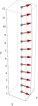
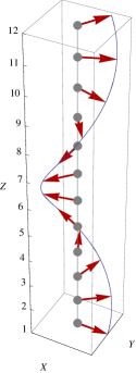
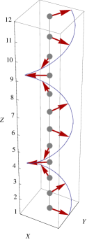
Figure 1: (Color online) Orientation, for a pure NESS in the Zeno regime, of the lattice spins of a driven $XXZ$ chain arranged along the $Z$ axis with boundary twisting in the $XY$ plane for winding number $m=0,1,2$ (left to right). The $Z$ labels indicate the lattice points along the chain. Parameters: $N=12$, $\Phi=\pi/3$.

Since Eqs. (5) and (9) satisfied by our $XY$-twisting solution are just necessary (but not sufficient) conditions for the NESS in the Zeno limit to be pure, one needs an independent check of the pureness of the found solution. A straightforward analytic computation for small system sizes $N\leq 7$ reveals that indeed the found NESS in the Zeno limit becomes pure exactly for the anisotropies (20), with two exceptions, namely, $\Phi=0$ and $\Delta=0$; see Appendix C. Moreover, we find that no other pure states in the Zeno limit exist. Thus, all solutions of Eqs. (5) and (8) for real-valued $\Delta$ are given by the factorized states (13) with anisotropy (20).

In Fig. 2 we show the von Neumann entropy $S=-\mathop{\mathrm{tr}}\limits(\rho_{\mathrm{NESS}}\log_{2}\rho_{\mathrm{NESS}})$ versus the anisotropy $\Delta$, in the Zeno limit and for finite $\Gamma$, obtained numerically for a system of four sites. In the Zeno limit, the NESS becomes pure, i.e., $S=0$, only at the points predicted by Eq. (20). For finite $\Gamma$, the NESS is always mixed. However, at the points (20), and for $\Gamma$ finite but larger and larger, $\rho_{\mathrm{NESS}}$ approaches the respective pure states arbitrarily closely.

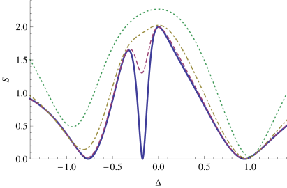
Figure 2: (Color online) The von Neumann entropy $S=-\mathop{\mathrm{tr}}\limits(\rho\log_{2}\rho)$ for $\rho=\rho_{\mathrm{NESS}}$ versus the $Z$-axis anisotropy $\Delta$, in a driven $XXZ$ chain with boundary twisting in the $XY$ plane. The dotted, dot-dashed and dashed lines correspond to finite dissipative couplings, $\Gamma=2,5,15$, respectively, while the thick line is the Zeno limit. Parameters: $N=4$, $\Phi=\pi/3$.

To find out if the pure states found in the Zeno regime are experimentally accessible, we have numerically calculated the minimal dissipation strength $\Gamma_{\epsilon}(m,N,\Phi)$ required to reach a pure NESS within a given tolerance $\epsilon$, and the relaxation time needed to establish the NESS, namely, the inverse gap $\lambda(\Gamma_{\epsilon})^{-1}$ of the spectrum of the Liouvillian $\mathcal{L}[\cdot]=-i\left[H,\cdot\right]+\Gamma\mathcal{D}[\cdot]$ at $\Gamma=\Gamma_{\epsilon}$. In practice, we define $\Gamma_{\epsilon}$ as the dissipation strength at which the von Neumann entropy of the corresponding NESS becomes equal to $\epsilon$; see Appendix D for details. Most remarkably, we find, on the base of a study of small-size systems ($N\leq 9$), that the optimal (minimized among all the winding numbers $m$ NotaCurrent ) $\Gamma_{\epsilon}$ decreases with $N$, making the effective “Zeno regime” more and more accessible as the system size increases; see Fig. 3. This somewhat counter-intuitive property follows from the fact that for longer chains, it becomes easier to freeze the boundary spins, i.e. to suppress their fluctuations, so that the effective Zeno regime is reached earlier. In compensation, the corresponding relaxation time increases with $N$; see Fig. 3. However, this increase is only polynomial, in accordance with the general observation made in Znidaric2015Gaps .

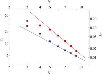
Figure 3: (Color online) Minimal dissipation strength $\Gamma_{\epsilon}$ needed to reach a pure state with accuracy $\epsilon=10^{-3}$ versus system size $N$ (dots, left-bottom axes). The solid line is the fit $\Gamma_{\epsilon}=94.8N^{-1.36}$. Gap $\lambda_{\Gamma_{\epsilon}}$ of the Liouvillian spectrum at $\Gamma=\Gamma_{\epsilon}$ versus system size $N$ (squares, right-top axes). The solid line is the fit $\lambda_{\Gamma_{\epsilon}}=9.42N^{-2.88}$. Parameters: $\Phi=\pi/3$, $\Delta=\cos(\Phi/(N-1))$.

III.2 Boundary twisting in the $XZ$ plane

Next we orient the boundary polarization in the $XZ$ plane, ${\vec{l}}_{L}=(\sin\theta_{L},0,\cos\theta_{L})$, ${\vec{l}}_{R}=(\sin\theta_{R},0,\cos\theta_{R})$. As before, we first solve Eq. (14), now taking $|\psi_{k}\rangle$ in the form

$$|\psi_{k}\rangle=\left(\begin{array}[]{l}\cos\frac{\theta_{k}}{2}\\ \sin\frac{\theta_{k}}{2}\end{array}\right),$$ (23)

which corresponds to a local spin polarization ${\vec{l}}_{k}=(\sin\theta_{k},0,\cos\theta_{k})$, and then restrict the found solution to meet Eqs. (5) and (9). As detailed in Appendix E, we have a NESS which can be of two kinds, corresponding to the orbital angles $\theta_{k}$ monotonically decreasing or increasing in the interval $]0,\pi[$; see Fig. 4. We never have a pure NESS with $\theta_{k}=0,\pi$ unless in the thermodynamic limit $N\rightarrow\infty$. For finite-size systems and given boundary polarizations in the $XZ$ plane, i.e., $\theta_{L}$, $\theta_{R}$, the NESS becomes pure in the Zeno limit and only for the anisotropy value,

$$\Delta(\theta_{L},\theta_{R})= \frac{1}{2}\left[\tan(\theta_{R}/2)/\tan(\theta_{L}/2)\right]^{1/(N-1)}$$

$$+\frac{1}{2}\left[\tan(\theta_{L}/2)/\tan(\theta_{R}/2)\right]^{1/(N-1)}.$$ (24)

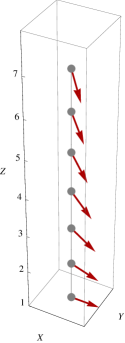
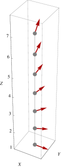
Figure 4: (Color online) As in Fig. 1 for boundary twisting in the $XZ$ plane and in correspondence to solutions with decreasing (left) and increasing (right) orbital angles. Parameters: $N=7$, $\theta_{L}=\pi/2$, $\theta_{R}=\pi/10$ (left), $\theta_{R}=\pi-\pi/10$ (right).

In Fig. 5, we show the dependence of the von Neumann entropy $S=-\mathop{\mathrm{tr}}\limits(\rho_{\mathrm{NESS}}\log_{2}\rho_{\mathrm{NESS}})$, obtained by numerically evaluating the NESS in a system of four sites for different values of the anisotropy. In the Zeno limit, the NESS becomes pure, i.e., $S=0$, at the point predicted by Eq. (24).

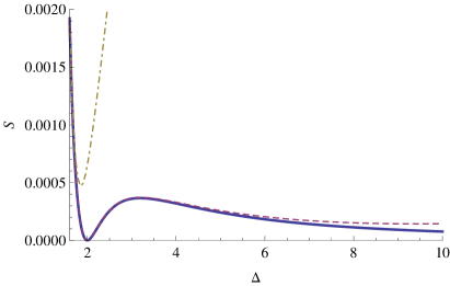
Figure 5: (Color online) The von Neumann entropy $S=-\mathop{\mathrm{tr}}\limits(\rho\log_{2}\rho)$ for $\rho=\rho_{\mathrm{NESS}}$ versus the $Z$-axis anisotropy $\Delta$, in a driven $XXZ$ chain with boundary twisting in the $XZ$ plane. Parameters: $N=4$, $\theta_{L}=\pi/2$, $\theta_{R}=\arctan(1/(15\sqrt{3}))$. The NESS is pure for a single value of the anisotropy, $\Delta=2$, given by Eq. (24). The dot-dashed and dashed lines are obtained for finite dissipative couplings, $\Gamma=30,370$, respectively, while the thick line is the Zeno limit.

IV Conclusions

To summarize, we have formulated a criterion for a nonequilibrium steady state of an open quantum system to be pure, in the Zeno limit, i.e., for asymptotically large dissipative coupling. The criterion is specified by Eqs. (5) and (8). Zeno-limit pure states are not reachable, in a strict mathematical sense, for any finite dissipative coupling. However, by applying a finite but large enough dissipative coupling, one can generate pure NESSs with arbitrary precision.

Using our criterion, in the Zeno regime we find two families of pure NESSs for the driven quantum $XXZ$ spin chain with boundary twisting in the $XY$ or $XZ$ plane, for values of the $Z$-axis anisotropy given by Eqs. (20) and (24), respectively. The criterion can be straightforwardly applied to generate pure steady states in other nonequilibrium quantum systems.

Our approach opens an interesting perspective in dissipative engineering of pure states. If, for given resources, preparing an exact pure steady state at finite dissipative strength is impossible (as it happens in our example of driven $XXZ$ chain), it may still be possible to generate a pure state in the Zeno limit. In practice, this means that at finite dissipation, a slightly mixed state will be produced, which, however, becomes infinitesimally close to a pure state as the dissipation is increased. The effective coupling needed to reach the “Zeno regime” depends on the chosen measure of pureness and the required precision and must be estimated in each case separately. In the example of the driven $XXZ$ model considered here, the effective Zeno regime is reached at very moderate dissipative couplings.

Appendix A Inverse of the Lindblad dissipator and secular conditions

The Lindblad operators $L_{1}\equiv\mathcal{L}_{L}$, $L_{2}\equiv\mathcal{L}_{R}$ have the form

$$L_{1}= \ [(\cos\theta_{L}\cos\varphi_{L})\sigma_{1}^{x}+(\cos\theta_{L}\sin\varphi_{L})\sigma_{1}^{y}$$

$$-(\sin\theta_{L})\sigma_{1}^{z}+i\sigma_{1}^{x}(-\sin\varphi_{L})+i\sigma_{1}^{y}(\cos\varphi_{L})]/2,$$

$$L_{2}= \ [(\cos\theta_{R}\cos\varphi_{R})\sigma_{N}^{x}+(\cos\theta_{R}\sin\varphi_{R})\sigma_{N}^{y}$$

$$-(\sin\theta_{R})\sigma_{N}^{z}+i\sigma_{N}^{x}(-\sin\varphi_{R})+i\sigma_{N}^{y}(\cos\varphi_{R})]/2.$$

The dissipator, $\mathcal{D}=\mathcal{D}_{L}+\mathcal{D}_{R}$, is the sum of the left and right dissipators

$$\mathcal{D}_{L}[\cdot]=L_{1}\cdot L_{1}^{\dagger}-\frac{1}{2}\{L_{1}^{\dagger}L_{1},\cdot\},$$

$$\mathcal{D}_{R}[\cdot]=L_{2}\cdot L_{2}^{\dagger}-\frac{1}{2}\{L_{2}^{\dagger}L_{2},\cdot\},$$

which are linear super-operators acting locally on a single qubit. The eigenbasis $\{\phi_{R}^{\alpha}\}_{\alpha=1}^{4}$ of the eigenproblem $\mathcal{D}_{R}[\phi_{R}^{\alpha}]=\lambda_{\alpha}\phi_{R}^{\alpha}$ is

$$\{\phi_{R}^{\alpha}\}=\{ 2\rho_{R},2\rho_{R}-I,-\sin\varphi_{R}\sigma^{x}+\cos\varphi_{R}\sigma^{y},$$

$$\cos\theta_{R}(\cos\varphi_{R}\sigma^{x}+\sin\varphi_{R}\sigma^{y})-\sin\theta_{R}\sigma^{z}\}$$

with the respective eigenvalues

$$\{\lambda_{\alpha}\}=\{0,-1,-\frac{1}{2},-\frac{1}{2}\}.$$

Here $I$ is a 2$\times$2 unit matrix, $\sigma^{x},\sigma^{y},\sigma^{z}$ are the Pauli matrices, and $\rho_{R}$ is the targeted spin orientation at the right boundary. Analogously, the eigenbasis and eigenvalues of the eigenproblem $\mathcal{D}_{L}[\phi_{L}^{\beta}]=\mu_{\beta}\phi_{L}^{\beta}$ are

$$\{\phi_{L}^{\beta}\}=\{ 2\rho_{L},2\rho_{L}-I,-\sin\varphi_{L}\sigma^{x}+\cos\varphi_{L}\sigma^{y},$$

$$\cos\theta_{L}(\cos\varphi_{L}\sigma^{x}+\sin\varphi_{L}\sigma^{y})-\sin\theta_{L}\sigma^{z}\},$$

$$\{\mu_{\beta}\}=\{0,-1,-\frac{1}{2},-\frac{1}{2}\},$$

where $\rho_{L}$ is the targeted spin orientation at the left boundary. Since the bases $\{\phi_{R}^{\alpha}\}$ and $\{\phi_{L}^{\beta}\}$ are complete, any matrix $\chi$ acting in the appropriate Hilbert space can be expanded as

$$\chi=\sum\limits_{\alpha=1}^{4}\sum\limits_{\beta=1}^{4}\phi_{L}^{\beta}\otimes\chi_{\beta\alpha}\otimes\phi_{R}^{\alpha}.$$ (25)

Indeed, let us introduce two complementary bases

$$\{\psi_{L,R}^{\alpha}\}=\{ I/2,\rho_{L,R}-I,(-\sin\varphi_{L,R}\sigma^{x}+\cos\varphi_{L,R}\sigma^{y})/2,$$

$$(\cos\theta_{L,R}(\cos\varphi_{L,R}\sigma^{x}+\sin\varphi_{L,R}\sigma^{y})$$

$$\quad-\sin\theta_{L,R}\sigma^{z})/2\},$$

trace-orthonormal to the $\{\phi_{L,R}^{\alpha}\}$, namely, $\mathop{\mathrm{tr}}\limits(\psi_{R}^{\gamma}\phi_{R}^{\alpha})=\delta_{\alpha\gamma}$ and $\mathop{\mathrm{tr}}\limits(\psi_{L}^{\gamma}\phi_{L}^{\beta})=\delta_{\beta\gamma}$. Then, the coefficients of the expansion (25) are given by

$$\chi_{\beta\alpha}=\mathop{\mathrm{tr}_{1,N}}\limits((\psi_{L}^{\beta}\otimes I^{\otimes_{N-1}})F(I^{\otimes_{N-1}}\otimes\psi_{R}^{\alpha})),$$

where $\mathop{\mathrm{tr}_{1,N}}\limits$ denotes the trace taken with respect to the first- and the last-spin spaces only. On the other hand, in terms of the expansion (25), the super-operator inverse $\mathcal{D}^{-1}=(\mathcal{D}_{L}+\mathcal{D}_{R})^{-1}$ is simply

$$(\mathcal{D}_{L}+\mathcal{D}_{R})^{-1}[\chi]=\sum\limits_{\alpha,\beta}\frac{1}{\lambda_{\alpha}+\mu_{\beta}}\phi_{L}^{\beta}\otimes\chi_{\beta\alpha}\otimes\phi_{R}^{\alpha}.$$

The above sum contains a singular term with $\alpha=\beta=1$, because $\lambda_{1}+\mu_{1}=0.$ To eliminate this singularity, one must require $\chi_{11}=\mathop{\mathrm{tr}_{1,N}}\limits\chi=0$, which is equivalent to the secular condition

$$P_{\ker\mathcal{D}}(\chi)=0,$$

where $P_{\Omega}$ denotes the orthogonal projector on $\Omega$.

We conclude that the existence of $\rho^{(k+1)}=\mathcal{D}^{-1}[i[H,\rho^{(k)}]]$ at order $k=0,1,2,\dots$ is granted if and only if

$$\mathop{\mathrm{tr}_{1,N}}\limits([H,\rho^{(k)}])=0.$$ (26)

Appendix B Stationary states with boundary twisting in the $XY$ plane

Assuming $\rho^{(0)}=|\Psi\rangle\langle\Psi|$ in the factorized form

$$|\Psi\rangle=|\psi_{1}\rangle\otimes|\psi_{2}\rangle\otimes\dots|\psi_{N}\rangle,$$

with

$$|\psi_{k}\rangle=\frac{1}{\sqrt{2}}\left(\begin{array}[]{c}e^{-i\frac{\varphi_{k}}{2}}\\ e^{i\frac{\varphi_{k}}{2}}\end{array}\right),\qquad k=1,\dots,N,$$

we look for a solution of the generalized divergence condition

$$h\left(|\psi_{k}\rangle\otimes|\psi_{k+1}\right\rangle)= \ \mu_{k}|\psi_{k}\rangle\otimes|\psi_{k+1}\rangle$$

$$+|U_{k}\rangle\otimes|\psi_{k+1}\rangle-|\psi_{k}\rangle\otimes|U_{k}\rangle,$$ (27)

where $h$ is the local density of the $H_{XXZ}$ Hamiltonian,

$$h=\frac{1}{2}\left(\sigma^{x}\otimes\sigma^{x}+\sigma^{y}\otimes\sigma^{y}+\Delta\left(\sigma^{z}\otimes\sigma^{z}-I\right)\right),$$

and $|U_{k}\rangle$ is a local unknown vector,

$$|U_{k}\rangle=\left(\begin{array}[]{c}u_{k}\\ v_{k}\end{array}\right).$$

Equation (27) is an overdetermined system of equations for $\mu_{k},u_{k},v_{k}$. The system does not admit a solution unless the $Z$-anisotropy parameter takes the value $\Delta=\cos(\varphi_{k+1}-\varphi_{k})$, which is possible only if the difference between any two consecutive angles along the chain is kept constant, $\varphi_{k+1}-\varphi_{k}=\gamma$. In this case, we have

$$\mu_{k}=4\sin\frac{\varphi_{k+1}-\varphi_{k}}{4}\cos^{2}\frac{\varphi_{k+1}-\varphi_{k}}{4},$$

$$u_{k}=-i\sqrt{2}\sin\frac{\varphi_{k+1}-\varphi_{k}}{4}\cos\frac{\varphi_{k+1}-\varphi_{k}}{2}e^{-i\frac{\varphi_{k+1}+\varphi_{k}}{4}},$$

$$v_{k}=i\sqrt{2}\sin\frac{\varphi_{k+1}-\varphi_{k}}{4}\cos\frac{\varphi_{k+1}-\varphi_{k}}{2}e^{i\frac{\varphi_{k+1}+\varphi_{k}}{4}}.$$

From the above solution, we compute

$$R_{k} =|U_{k}\rangle\langle\psi_{k}|-|\psi_{k}\rangle\langle U_{k}|=\frac{i}{2}\sigma^{z}\sin(\varphi_{k+1}-\varphi_{k}),$$

$$\tilde{R}_{k} =|U_{k-1}\rangle\langle\psi_{k}|-|\psi_{k}\rangle\langle U_{k-1}|=\frac{i}{2}\sigma^{z}\sin(\varphi_{k}-\varphi_{k-1}).$$

It is straightforward to check that the system of equations,

$$\sum_{k=1}^{N-1}\left(\mu_{k}-\mu_{k}^{*}\right)=0,$$ (28a)

$$R_{k}=\tilde{R}_{k},\qquad k=1,\dots,N,$$ (28b)

$$\mathop{\mathrm{tr}}\limits R_{1}=\mathop{\mathrm{tr}}\limits\tilde{R}_{N}=0,$$ (28c)

is then satisfied. Since Eq. (28) has been demonstrated to be equivalent to $P_{\ker\mathcal{D}}([H,|\Psi\rangle\langle\Psi|])=0$, we conclude that the found solution meets the necessary condition of our Zeno regime pure NESS criterion. To meet the other condition, namely, $\mathcal{D}[|\Psi\rangle\langle\Psi|]=0$, we just need to satisfy the boundary conditions $\varphi_{1}=0$ and $\varphi_{N}=\Phi$. This is accomplished by choosing

$$\gamma=\gamma(\Phi,m)=(\Phi+2\pi m)/(N-1),$$

with $m=0,1,\dots,N-2$.

Appendix C Analytic calculation of the Zeno NESS for small sizes and boundary twisting in the $XY$ plane

Solving the secular conditions (8) for $k=0,1$, we compute the analytic form of $\rho_{NESS}(N,\Delta,\Phi)$ for small system sizes $N$, and calculate the pureness parameter,

$$f(N,\Delta,\Phi)=\mathop{\mathrm{tr}}\limits[\rho_{NESS}(N,\Delta,\Phi)^{2}]-1.$$

Note that the state $\rho_{NESS}$ is pure if and only if $f=0$. We obtain

$$f(3,\Delta,\Phi)=-\frac{\left(-T_{2}(\Delta)+\cos(\Phi)\right)^{2}}{2\left(2\Delta^{2}+\cos(\Phi)+1\right)^{2}},$$

$$f(4,\Delta,\Phi)=-\left(-T_{3}(\Delta)+\cos(\Phi)\right)^{2}\frac{P_{4}}{D_{4}},$$

$$f(5,\Delta,\Phi)=-\left(-T_{4}(\Delta)+\cos(\Phi)\right)^{2}\frac{P_{5}}{D_{5}},$$

$$\vdots$$

where $T_{n}(\cos x)=\cos(nx)$ are Chebyshev polynomials of the first kind,

$$T_{2}(x)=-1+x^{2},$$

$$T_{3}(x)=-3x+4x^{3},$$

$$T_{5}(x)=1-8x^{2}+8x^{4},$$

$$\vdots$$

and, for instance,

$$P_{4}= 16\Delta^{6}+56\Delta^{4}+4\left(10\Delta^{2}+3\right)\Delta\cos(\Phi)$$

$$+30\Delta^{2}+3\cos(2\Phi)+3,$$

$$Q_{4}= 2\left(16\Delta^{6}+12\Delta^{4}+4\left(5\Delta^{2}+2\right)\Delta\cos(\Phi)\right.$$

$$+\left.14\Delta^{2}+\cos(2\Phi)+1\right)^{2}.$$

Substituting $\Delta=\cos\gamma$ into the above expressions for $f$, we obtain

$$f(3,\cos\gamma,\Phi)=-\frac{(\cos(2\gamma)-\cos(\Phi))^{2}}{2(\cos(2\gamma)+\cos(\Phi)+2)^{2}},$$

$$f(4,\cos\gamma,\Phi)=-\left(\cos(3\gamma)-\cos(\Phi)\right)^{2}\frac{P_{4}}{D_{4}},$$

$$f(5,\cos\gamma,\Phi)=-\left(\cos(4\gamma)-\cos(\Phi)\right)^{2}\frac{P_{5}}{D_{5}},$$

$$\vdots$$

Extrapolating for arbitrary $N$, we get $\cos((N-1)\gamma)=\cos(\Phi)$ as a pure NESS condition, yielding

$$\gamma(\Phi,m)=(\Phi+2\pi m)/(N-1),\qquad m=0,1,...,N-2,$$

as well as

$$\Delta(\Phi,m)=\cos\left(\gamma(\Phi,m)\right)=\cos\left(\frac{\Phi+2\pi m}{N-1}\right).$$ (29)

Independently, we verify that the anisotropy values given by Eq. (29) exhaust the solutions of the equations $f(N,\Delta,\Phi)=0$ for $\Delta$ being real. Points of non-analyticity of the functions $f(N,\Delta,\Phi)$, e.g. $f(3,0,\pi)=0/0$, correspond to exceptions and need to be analyzed separately.

Exception (a) $\Phi=0$. This case corresponds to a full boundary alignment, i.e. to the absence of a boundary gradient. The Zeno NESS is pure only for $\Delta=1$ for $N$ even, which corresponds to $m=0$ in Eq. (29), and $\Delta=\pm 1$ for $N$ odd, corresponding to $m=0,(N-1)/2$ in Eq. (29). The $\Delta=1$ solution represents a trivial factorized state with all spins polarized in the $X$ direction. This homogeneous state remains a NESS for any finite value of $\Gamma$.

Exception (b) $\Delta=0$. Whenever among the critical anisotropy values (29), a free fermion point $\Delta=0$ appears, the respective NESS at $\Delta=0$ is not a pure state, but a fully mixed state, apart from the boundaries, $\rho_{NESS}=\rho_{L}\otimes(I/2)^{\otimes_{N-2}}\otimes\rho_{R}$. The peculiarity of this exception results from the fact that the Zeno limit $\Gamma\rightarrow\infty$ and the free-fermion limit $\Delta\rightarrow 0$ do not commute, with the reason being the existence of an extra symmetry of the NESS at $\Delta\rightarrow 0$; see 2012XYtwist for an elaborate treatment of a $\Phi=\pi/2$ case.

Appendix D Minimal dissipation strength $\Gamma_{\epsilon}(m,N,\Phi)$

For system sizes $3\leq N\leq 9$, we have numerically calculated $\rho_{\mathrm{NESS}}(\Gamma)$, namely the NESS of the Liouvillian $-i[H,\cdot]+\Gamma\mathcal{D}[\cdot]$, where $H$ is the Hamiltonian of the $XXZ$ model and $\mathcal{D}=\mathcal{D}_{L}+\mathcal{D}_{R}$ is the dissipator described in Appendix A, for several finite dissipation strengths $\Gamma$. In the case of boundary twisting in the $XY$ plane, the von Neumann entropy $S(\Gamma)=-\mathop{\mathrm{tr}}\limits(\rho_{\mathrm{NESS}}(\Gamma)\log_{2}\rho_{\mathrm{NESS}}(\Gamma))$ corresponding to the NESS obtained for $m=0$ and $\Phi=\pi/3$ is plotted in Fig. 6 as a function of $\Gamma$. We see that, for any $N$, $S(\Gamma)$ decreases monotonously to 0 by increasing $\Gamma$, approximately as $\Gamma^{-2}$ for $\Gamma$ large. As is natural, we define the minimal dissipation strength $\Gamma_{\epsilon}(m,N,\Phi)$ required to reach a pure NESS within a given tolerance $\epsilon$ as the unique solution of

$$S(\Gamma_{\epsilon})=-\mathop{\mathrm{tr}}\limits\left[\rho_{NESS}(\Gamma_{\epsilon})\log_{2}\rho_{NESS}(\Gamma_{\epsilon})\right]=\epsilon,$$

which is plotted in Fig. 3 of the main text.

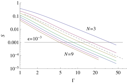
Figure 6: (Color online) The von Neumann entropy $S(\Gamma)=-\mathop{\mathrm{tr}}\limits[\rho_{\mathrm{NESS}}(\Gamma)\log_{2}\rho_{\mathrm{NESS}}(\Gamma)]$ corresponding to the NESS calculated for $m=0$ and $\Phi=\pi/3$ in the case of boundary twisting in the $XY$ plane and for system size $N$ from 3 (top) to 9 (bottom). The dashed line is the eye-guide $S\sim\Gamma^{-2}$ while the horizontal solid line is the tolerance value $S=10^{-3}$.

Appendix E Stationary states with boundary twisting in the $XZ$ plane

Here, we solve Eq. (14) taking $|\psi_{k}\rangle$ in the form

$$|\psi_{k}\rangle=\left(\begin{array}[]{l}\cos\frac{\theta_{k}}{2}\\ \sin\frac{\theta_{k}}{2}\end{array}\right).$$

It is convenient to denote

$$\kappa_{k}=\left(\tan(\theta_{k+1}/2)\right)/\left(\tan(\theta_{k}/2)\right).$$

We find that if the $Z$-anisotropy has the value $2\Delta=\kappa_{k}+\kappa_{k}^{-1}$, Eq. (14) has the solution

$$\mu_{k}=-\frac{\left(\cos\frac{\theta_{k}+3\theta_{k+1}}{2}-\cos 3\frac{\theta_{k}+\theta_{k+1}}{2}\right)^{2}}{\sin\theta_{k}\sin\theta_{k+1}},$$

$$u_{k}=\frac{\cos\frac{\theta_{k+1}}{2}-\cos\frac{\theta_{k}}{2}}{\sin\frac{\theta_{k}}{2}\sin\frac{\theta_{k+1}}{2}}\cos^{2}\frac{\theta_{k}+\theta_{k+1}}{4},$$

$$v_{k}=\frac{\sin\frac{\theta_{k+1}}{2}-\sin\frac{\theta_{k}}{2}}{\cos\frac{\theta_{k}}{2}\cos\frac{\theta_{k+1}}{2}}\sin^{2}\frac{\theta_{k}+\theta_{k+1}}{4}.$$

From the above solution, we compute

$$R_{k}=|U_{k}\rangle\langle\psi_{k}|-|\psi_{k}\rangle\langle U_{k}|=ib_{k}\sigma^{y},$$

$$\tilde{R}_{k}=|U_{k-1}\rangle\langle\psi_{k}|-|\psi_{k}\rangle\langle U_{k-1}|=i\tilde{b}_{k}\sigma^{y},$$

with

$$b_{k} =(\cos\theta_{k+1}-\cos\theta_{k})/\sin\theta_{k+1},$$

$$\tilde{b}_{k} =(\cos\theta_{k}-\cos\theta_{k-1})/\sin\theta_{k-1}.$$

Conditions (15), i.e., $P_{\ker\mathcal{D}}([H,|\Psi\rangle\langle\Psi|])=0$, are thus satisfied if $\kappa_{k}+\kappa_{k}^{-1}=2\Delta$ and $\tilde{b}_{k}=b_{k}$ for all $k$. The latter condition after some algebra gives

$$\kappa_{k}^{-1}+\kappa_{k-1}=\kappa_{k}+\kappa_{k-1}^{-1}.$$ (30)

Notice that since $\kappa_{k}$ are real numbers, $|\Delta|>1$. There are two independent solutions of Eq. (30), namely, $\kappa_{k}=z_{\pm}$, where $z_{\pm}=\Delta\pm\sqrt{\Delta^{2}-1}$ are the roots of the quadratic equation $z+1/z=\Delta$. To meet the condition $\mathcal{D}[|\Psi\rangle\langle\Psi|]=0$, we require $\theta_{1}=\theta_{L}$ and $\theta_{N}=\theta_{R}$.

The solutions with $\kappa_{k}=z_{\pm}$ describe orbital angles $\theta_{k}$ monotonically decreasing or increasing in the interval $]0,\pi[$. Note that we never have a pure NESS with $\theta_{k}=0,\pi$, unless in the thermodynamic limit $N\rightarrow\infty$. In conclusion, for finite-size systems and given boundary polarizations in the $XZ$ plane, we have one NESS in correspondence to the anisotropy value,

$$\Delta(\theta_{L},\theta_{R})= \frac{1}{2}\left[\tan(\theta_{R}/2)/\tan(\theta_{L}/2)\right]^{\frac{1}{N-1}}$$

$$+\frac{1}{2}\left[\tan(\theta_{L}/2)/\tan(\theta_{R}/2)\right]^{\frac{1}{N-1}}.$$ (31)

References

- (1) A. Beige, D. Braun, B. Tregenna and P. L. Knight Phys. Rev. Lett. 85, 1762 (2000).
- (2) M. J. Kastoryano, F. Reiter, and A. S. Sørensen, Phys. Rev. Lett. 106, 090502 (2011).
- (3) Y. Lin, J. P. Gaebler, F. Reiter, T. R. Tan, R. Bowler, A. S. S rensen, D. Leibfried and D. J. Wineland, Nature (London) 504, 415 (2013).
- (4) S. Shankar, M. Hatridge, Z. Leghtas, K. M. Sliwa, A. Narla, U. Vool, S. M. Girvin, L. Frunzio, M. Mirrahimi, M. H. Devoret, Nature (London) 504, 419 (2013).
- (5) D. Kienzler, H.-Y. Lo, B. Keitch, L. de Clercq, F. Leupold, F. Lindenfelser, M. Marinelli, V. Negnevitsky, J. P. Home, Science 347, issue 6217, 53 (2015).
- (6) F. Ticozzi and L. Viola, Philos. Trans. R. Soc A 370 5259 (2012).
- (7) F. Verstraete, M. M. Wolf and J. I. Cirac, Nat. Phys. 5, 633 (2009).
- (8) H. Häffner, C. F. Roos and R. Blatt, Phys. Reports 469, 155 (2008), and references therein.
- (9) P. Schindler, M. Muller, D. Nigg, J. T. Barreiro, E. A. Martinez, M. Hennrich, T. Monz, S. Diehl, P. Zoller and R. Blatt, Nature Physics 9, 361 (2013).
- (10) Hanna Krauter, Christine A. Muschik, Kasper Jensen, Wojciech Wasilewski, Jonas M. Petersen, J. I. Cirac, and Eugene S. Polzik, Phys. Rev. Lett. 107, 080503 (2011).
- (11) K. Stannigel, P. Rabl and P. Zoller, New Journal of Physics 14 (2012) 063014.
- (12) S. Zippilli, M. Paternostro, G. Adesso and F. Illuminati, Phys. Rev. Lett. 110, 040503 (2013).
- (13) F. Pastawski, L. Clemente, and J. I. Cirac, Phys. Rev. A 83, 012304 (2011).
- (14) J. I. Cirac, A. S. Parkins, R. Blatt and P. Zoller, Phys. Rev. Lett. 70, 556 (1993).
- (15) N. Yamamoto, Phys. Rev. A 72, 024104 (2005).
- (16) B. Kraus, H. P. Buchler, S. Diehl, A. Kantian, A. Micheli and P. Zoller, Phys. Rev. A 78, 042307 (2008).
- (17) S. Diehl, A. Micheli, A. Kantian, B. Kraus, H. P. Buchler, and P. Zoller, Nature Physics 4, 878 (2008).
- (18) C. Cormick, A. Bermudez, S. F. Huelga, and M. B. Plenio, New Journal of Physics 15, 073027 (2013).
- (19) The necessary and sufficient condition for a NESS to be pure can always be brought to the form (3) by a re-partitioning of and ; see Yamamoto05 ; ZollerPRA08 .
- (20) S. Diehl, A. Tomadin, A. Micheli, R. Fazio and P. Zoller, Phys. Rev. Lett. 105, 015702 (2010).
- (21) K. Koshino and A. Shimizu, Phys. Reports 412,Issue 4, 191 (2005).
- (22) M. C. Fischer, B. Gutiérrez-Medina, and M. G. Raizen, Phys. Rev. Lett. 87, 040402 (2001).
- (23) F. Schäfer, I. Herrera, S. Cherukattil, C. Lovecchio, F. S. Cataliotti, F. Caruso and A. Smerzi, Nat. Commun. 5, 3194 (2014).
- (24) P. Facchi and S. Pascazio, Phys. Rev. Lett. 89, 080401 (2002); J. Phys. A 41, 493001 (2008).
- (25) H.-P. Breuer and F. Petruccione, The Theory of Open Quantum Systems (Oxford University Press, Oxford, 2002).
- (26) M. B. Plenio and P. L. Knight, Rev. Mod. Phys. 70, 101 (1998).
- (27) S. R. Clark, J. Prior, M. J. Hartmann, D. Jaksch and M. B. Plenio, New J. Phys. 12, 025005 (2010).
- (28) T. Prosen, Phys. Rev. Lett. 107, 137201 (2011).
- (29) D. Karevski, V. Popkov and G. M. Schütz, Phys. Rev. Lett. 110, 047201 (2013).
- (30) V. Popkov, D. Karevski and G. M. Schütz, Phys. Rev. E 88, 062118 (2013).
- (31) T. Prosen, J. Phys. A: Math. Theor. 48, 373001 (2015).
- (32) V. Popkov, J. Stat. Mech. 2012, P12015 (2012).
- (33) V. Popkov, and M. Salerno, J. Stat. Mech. 2013, P02040 (2013).
- (34) We find that the optimal corresponds to the smallest steady-state current which, for , gives for even and for odd.
- (35) M. Žnidarič, Phys. Rev. E 92, 042143 (2015).