Rapid variability at very high energies in Mrk 501

Abstract:

A major flaring state of the BL Lac object Mrk 501 was observed by the High Energy Stereoscopic System (H.E.S.S.) in June, 2014. Flux levels higher than one Crab unit were recorded and rapid variability at very high energies ($\sim$2-20 TeV) was revealed. The high statistics afforded by the flares allowed us to probe the presence of minutes timescale variability and study its statistical characteristics exclusively at TeV energies owing to the high energy threshold of approximately 2 TeV. Doubling times of a few minutes are estimated for fluxes greater than 2 TeV. Statistical tests on the light curves show interesting temporal structure in the variations including deviations from a normal flux distribution similar to those found in the PKS 2155-304 flare of July 2006, at nearly an order of magnitude higher threshold energy. Rapid variations at such high energies put strong constraints on the physical mechanisms in the blazar jet.

1 Introduction

Markarian 501 (Mrk 501) at $z=0.034$ is a well studied high-frequency peaked BL Lacertae (HBL) object. Historically, it has shown highly variable emission in wavelengths ranging from radio to very high energy (VHE, E ¿ 100 GeV) gamma-rays. It was first detected above 300 GeV by the Whipple Observatory in 1996 [1]. Since then it has been observed several times at TeV energies [2, 3, 4, etc.]. It has shown VHE variability down to minute timescales between 0.15-10 TeV as reported by MAGIC in [4]. TeV observations coupled with X-ray observations usually put strong constraints on the source magnetic field and Doppler factors within the context of a homogenous synchrotron self-Compton model [5]. Observations by the High Energy Stereoscopic System (H.E.S.S.) have been carried out in four periods between 2004 and 2014 [6]. In this proceeding, the focus will be on the 2014 observations, which includes the strongest flare ever detected by H.E.S.S. Afforded by the unique data set, the VHE variability is investigated. It is at energy scales higher than reported before and the aim is to improve and extend constraints on the source emission mechanisms. Also, comparisons with the 2006 flare of PKS 2155-304 [7] are instructive in looking for general features in the temporal structure of the emission and therefore for potential principles underlying the physics of jet emission.

2 Rapid flux variations at very high energies

The 2014 H.E.S.S. observations of Mrk 501 at large Zenith angles (¿60^∘) were performed as a target of opportunity following fluxes over 1 Crab unit reported by the FACT collaboration. Nightly fluxes above 2 TeV ranging from $\sim$3 to 40$\times$10^-12 cm^-2s^-1 were recorded between the nights of June 19-25. On the night of June 23-24 a large flare was detected comprising the highest fluxes of Mrk 501 recorded by H.E.S.S. This study focuses on the temporal characteristics of the 2014 data and explores physical constraints that may be derived with time series analysis studies. More information about the spectral analysis of the whole dataset as well as the multiwavelength context can be found in [6].

The observations during this period comprise of data from all five H.E.S.S. telescopes CT1 to CT5. In order to have an homogeneous dataset and eliminate variance due to two telescope types, only information from CT1-4 has been extracted from the data. The livetime is $\sim$7.7 hours (6.8  after acceptance correction). The mean Zenith angle is 63.7^∘. The analysis was performed with the Model analysis method [8] with $Loose$ cuts. The background estimation was made using the $Reflected\ Region\ Background$ method [9]. As a result of the high Zenith angles, the energy threshold is $\gtrsim$  2 TeV. Therefore, the striking feature of these observations is that the light curve obtained is exclusively at TeV energies. Consequently, the variability detected is also exclusively at TeV energies, unlike previous studies where the variations were dominated by fluxes at energies of few hundreds of GeVs.

Variations at TeV energies are found down to a few minutes (¡ 10 minutes), as shown in Fig. 1. The lightcurve covers the days from MJD 56828 to 56833 and shows a strong flaring event during MJD 56831-56832. A zoom into the peak of the flare state is shown in Fig. 2. Using the median energy of the photons above 2 TeV the lightcurve is divided into 2 bands: $2.0-4.5$ TeV and $E>4.5$ TeV. As shown in Fig. 1 and more sharply in Fig. 2, short timescale variations are seen at energies $>2$ TeV as well as $>4.5$ TeV. The fractional variability $F_{\rm var}$ is used to quantify timescales following [10]. It is the excess variance scaled down by the mean flux as,

$$F_{\rm var}=\sqrt{\left(\frac{\phi^{2}-\langle\sigma_{\rm err}^{2}\rangle}{\phi_{\rm mean}^{2}}\right)}$$ (1)

The values are obtained for each of the bands shown in the figures. For $E>2$ TeV, $F_{\rm var}\sim 1.1\pm 0.3\times 10^{-1}$. Such short timescale VHE variability has also been observed by H.E.S.S. in another HBL source, PKS 2155-304 ($z=0.116$), whose temporal structure has been studied in detail [7, 11]. The flaring state of PKS 2155-304 in July 2006 had higher VHE fluxes than those of Mrk 501 in June 2014; this included two nights, MJD 53944 and MJD 53946 where the flux levels were $\sim$ 9 and $\sim$ 12 times that of the Crab Nebula at these energies. Therefore, constraining the temporal structure for the Mrk 501 flares and thus the VHE emission mechanisms appears more challenging. On the other hand, the spectral characteristics imply that the flare in PKS 2155-304 was dominated by fluxes at energies lower than 1 TeV. In the following, a preliminary investigation of the variability characteristics of Mrk 501 will be made, together with the comparison, when appropriate, with the results for PKS 2155-304 reported in [7] in order to understand if the emission mechanisms are similar and possibly extend over a broad range of energies. Some techniques used for the temporal studies of PKS 2155-304 are used here. Flux doubling times defined as in [12] are used as an estimator for the variability timescales. It is defined as

$$T_{\rm 2}^{j,k}=|\bar{\phi}\ \Delta T/\Delta\phi|$$ (2)

where $\Delta\phi=\phi_{j}-\phi_{k}$ and $\Delta T=T_{j}-T_{k}$ are the flux and time differences between the jth and kth data points, respectively, and $\bar{\phi}=\frac{\phi_{j}+\phi_{k}}{2}$ is the corresponding mean flux. The entire data set from June 19-25th is used for this analysis. The time binning is selected ensuring a minimum significance ($\gtrsim 3\sigma$) per bin during the flare.

The minimum variability timescale computed by this method is $T_{\rm min}<$ 10 minutes. The minimum of the values of time difference between all pairs $T_{2,\rm min}$, is computed to be $\approx 6.5\pm 2.9$ minutes. The mean of the 5 smallest values of these pairwise time differences is $\tilde{T}_{2,\rm min}\approx 6.6\pm 2.8$ minutes. The pairs chosen have a relative error $\leq 50\%$ obtained by propagating the error in the fluxes. This gives a rough estimate of the variability timescales, even though it is understood that this is not fully robust and sensitive to the time binning. In this case the bin size used was 4 mins. So far, variations at such timescales observed in Mrk 501 were dominated by energies below the threshold of this observation ($\sim$2 TeV). Figure 2 shows a zoom-in to the peak of the flare. This clearly shows variability at a few minute timescales for both fluxes above 2 and 4.5 TeV.

Figure 1: The figure shows the variations in the flux for Mrk 501 over the course of the few days of activity in June 2014. The light curves are binned runwise. The fluxes are above the analyses threshold of $\approx$ 2 TeV. The flux points in the figure are shown with 1-$\sigma$ error bars.

Figure 2: The figure shows a zoom into the peak of the flare on June 23-24. As in the previous figure, the panels are $\phi$(¿ 2 TeV), $\phi$(2-4.5 TeV) and $\phi$(¿4.5 TeV). It is evident that there is variation on a few minute timescales at every energy range including the one above 4.5 TeV. The 1-$\sigma$ error bars are shown.

3 Underlying TeV flux distribution

The underlying flux probability distribution function (PDF) gives hints as to the emission mechanisms. The PDF is represented simply by the histogram of the fluxes. If the PDF is lognormal, this suggests a multiplicative emission process as opposed to an additive process. In principle, this would be a characteristic of a ”cascade-like” process. For PKS 2155-304 strong evidence for log-normality was found in the July 2006 flare data and in general in multiwavelength data [13], revealing a clear preference for a normal distribution of the logarithm of fluxes rather than the fluxes themselves. This could possibly point to very interesting physical implications [14, 15]. Thus, the distribution of TeV fluxes shown in figure 1 has been tested for the same effect in Mrk 501. It is found that even in this case, fluxes tend to prefer a log-normal distribution as shown in figure 3. This is based on a chisquare fit of both the distribution of fluxes as well as the logarithm of fluxes using the Gaussian function of form, $\frac{A}{\sqrt{2\ \pi\ \sigma^{2}}}\exp(-\ (x-\mu)^{2}/2\ \sigma^{2})$. There are 15 flux bins in each case with 3 bins per linear (or logarithmic) unit interval. The values of the reduced chi-square $\chi^{2}/\nu$ are in fact $22/8$ (probability $\sim 5\times 10^{-3}$) and $13/10$ (probability $\sim$0.2) for the distribution of fluxes and their logarithmic values, respectively. The log fluxes follow the normal distribution with normalisation $A=36.4\pm 4.0$, $\sigma=0.7\pm 1.8\times 10^{-1}$ and mean, $\mu=1.1\pm 0.2$ with a probability of $\sim 5\times 10^{-3}$ of exceeding $22/8$. The best fit values for a normal distribution of the fluxes themselves are $A=29.1\pm 3.4$, $\sigma=0.8\pm 0.1$ and mean, $\mu=0.5\pm 0.1$ with a probability of $\sim 0.2$ of exceeding $13/10$. Therefore, fluxes statistically prefer a lognormal distribution. To determine more clearly, whether the underlying distribution is indeed log-normal, one would have to simulate light curves with both normal and lognormal flux distributions along with the appropriate power spectral density as in [16] and then perform a full likelihood analysis. This goes beyond the scope of the current proceedings and will be the subject of a future paper.

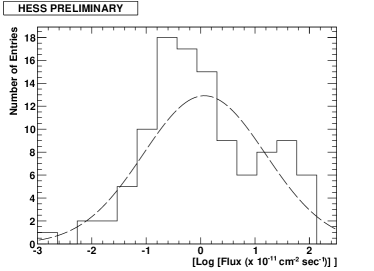
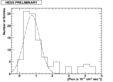
Figure 3: The figure shows the distribution of TeV fluxes from the entire duration of the flare in Mrk 501. To the left is the distribution of the fluxes and to the right the logarithm of the fluxes. There is a statistical preference towards a log-normal distribution as suggested by the reduced chi-squared values. This hints to a lognormal behaviour at TeV energies.

4 Power Spectral Density

An important characteristic central to the temporal structure of the variations in the emission of a source is the power spectral density (PSD) [16, 17]. The PSD represents the density of temporal fluctuations expressed in the frequency domain. For AGNs, the PSD is often a power-law ($\propto\nu^{-\alpha}$), with different flaring and quiescent states characterised by different powers.

Figure 4: The figure shows the PSD for fluxes $\phi$(¿ 2 TeV) binned at 4 minutes. The red line represents a single power law fit to the data - this suggests that above $\nu\gtrsim(1-2)\times 10^{-3}$ Hz, a simple power law is no longer a good description of the data. The error bars are computed analytically assuming Gaussian uncertainties using [17].

In the observations of June 2014, the periodogram is used as an estimator of the PSD [16]. The PSD of the data points is computed and can be described by a simple power law given by,

$$P(\nu)=A\ \nu^{-\alpha}$$ (3)

, where A is the proportionality constant and $\alpha$ is the index. The best fit values are $A=10^{-3.9\pm 1.1}$ and $\alpha=-1.7\pm 0.4$ with a reduced chisquare value of 1.4 for 52 degrees of freedom. This corresponds to a probability of $\sim 4.5\times 10^{-2}$. The best fit is shown by the red line in the figure 4. The error bars are computed using the analytical formula in [17]. This computation assumes that the data have Gaussian uncertainties. The errors are larger for Mrk 501 than for PKS 2155-304 as expected given the comparison of statistics between the two flaring episodes, necessitating simulations for drawing robust conclusions. It is evident from the figure that, such a simple power law red noise spectrum represents a reasonable fit up to frequencies of $\approx(1-2)\times 10^{-3}$ Hz, after which the scatter in the data weakens the constraints. Given the binsize of 4 minutes, it is expected that the fluctuations at frequencies higher than $1/2\times(f_{\rm sampling})$ will be suppressed. Furthermore, with the noise in the data above this frequency, it is difficult to constrain the shape of the PSD beyond this frequency. The presence of gaps in the lightcurve adds to the difficulty in placing constraints in general without performing simulations. The shape depends on the state of emission and thus constrains the mechanisms. In order to do this robustly, one again needs to perform a full likelihood analysis with simulated light curves and test for the likelihood of a simple power law describing the data.

5 Conclusions and Discussion

The flare of June 2014 in Mrk 501 was quite unprecedented in that it showed fast variations (on a few minutes timescales) at purely TeV energies. This provides us with the unique opportunity to test the characteristics of the emission processes in Mrk 501 at higher energies than seen till date for this source. Our analysis reveals that the TeV flux variations tend to favour a lognormal distribution which along with the inferred variability timescales could offer important clues as to a hadronic or leptonic origin. In principle, log-normality is suggestive of a multiplicative process and may be a natural outcome of a ”cascade-like” hadronic scenario or an intrinsic jet-disk connection, while generally fast variability is more easily accommodated in a leptonic context. Combined with observations at other wavelengths such as X-rays, these results will thus help to put further constraints on the magnetic field, the size and extent of the emission region and indeed the relative importance of hadronic versus leptonic processes as well as the applicability of different model assumptions, e.g. [18, 19, 20]. The inferred power spectral density is consistent with a single power law up to a certain frequency beyond which the scatter does not allow the PSD to be well constrained. The index of $\sim\ 1.7$ derived here for Mrk 501 is similar to the red-noise index of $\sim 2$ derived for PKS 2155-304 [14]. The onset of scatter may simply be a result of noise due to background fluctuations or a limitation due to lack of significant bins. Furthermore, presence of gaps in the lightcurve prevent putting definitive constraints. To assess this in more detail, a more sophisticated statistical treatment will be needed which will be presented elsewhere.

6 Acknowledgments

The support of the Namibian authorities and of the University of Namibia in facilitating the construction and operation of H.E.S.S. is gratefully acknowledged, as is the support by the German Ministry for Education and Research (BMBF), the Max Planck Society, the German Research Foundation (DFG), the French Ministry for Research, the CNRS-IN2P3 and the Astroparticle Interdisciplinary Programme of the CNRS, the U.K. Science and Technology Facilities Council (STFC), the IPNP of the Charles University, the Czech Science Foundation, the Polish Ministry of Science and Higher Education, the South African Department of Science and Technology and National Research Foundation, and by the University of Namibia. We appreciate the excellent work of the technical support staff in Berlin, Durham, Hamburg, Heidelberg, Palaiseau, Paris, Saclay, and in Namibia in the construction and operation of the equipment. The support of AvH foundation is also acknowledged. This research used lightcurve simulation codes provided by Physics and Astronomy, University of Southampton available at https://github.com/samconnolly/DELightcurveSimulation for computation of the PSD and the analytical expressions from the thesis of Jonathan Biteau for the PSD errors.

References

- [1] J. Quinn and J. Akerlof, C. W. and…Zweerink, Detection of Gamma Rays with E ¿ 300 GeV from Markarian 501, ApJ 456 (Jan., 1996) L83.
- [2] F. Aharonian and A. G. a. Akhperjanian, The temporal characteristics of the TeV gamma -emission from MKN 501 in 1997. II. Results from HEGRA CT1 and CT2, A&A 349 (Sept., 1999) 29–44, [astro-ph/9901284].
- [3] D. Huang, A. Konopelko, and for the VERITAS collaboration, VERITAS Observations of Mkn 501 in 2009, ArXiv e-prints (Dec., 2009) [arXiv:0912.3772].
- [4] J. Albert and J. Aliu, E. and…Zapatero, Variable Very High Energy -Ray Emission from Markarian 501, %2C(Astrophys. J. (669) (Nov., 2007) 862–883, [astro-ph/0702008].
- [5] F. Tavecchio, L. Maraschi, and G. Ghisellini, Constraints on the Physical Parameters of TeV Blazars, %2C(Astrophys. J. (509) (Dec., 1998) 608–619, [astro-ph/9809051].
- [6] G. Cologna, N. Chakraborty, M. Mohamed, and for the H. E. S. S. Collaboration, Spectral characteristics of Mrk 501 during the 2012 and 2014 flaring states, Proc. of the 34th ICRC (ICRC2015), The Hague, (Netherlands) (2015).
- [7] H.E.S.S. Collaboration and H. S. Abramowski, A. and..Zechlin, VHE -ray emission of PKS 2155-304: spectral and temporal variability, A&A 520 (Sept., 2010) A83, [arXiv:1005.3702].
- [8] M. de Naurois and L. Rolland, A high performance likelihood reconstruction of -rays for imaging atmospheric Cherenkov telescopes, Astroparticle Physics 32 (Dec., 2009) 231–252, [arXiv:0907.2610].
- [9] D. Berge, S. Funk, and J. Hinton, Background modelling in very-high-energy -ray astronomy, A&A 466 (May, 2007) 1219–1229, [astro-ph/0610959].
- [10] S. Vaughan, R. Edelson, R. S. Warwick, and P. Uttley, On characterizing the variability properties of X-ray light curves from active galaxies, MNRAS 345 (Nov., 2003) 1271–1284, [astro-ph/0307420].
- [11] F. Aharonian and A. A. Akhperjanian, A. G. and..Zdziarski, An Exceptional Very High Energy Gamma-Ray Flare of PKS 2155-304, ApJ 664 (Aug., 2007) L71–L74, [arXiv:0706.0797].
- [12] Y. H. Zhang and C. M. Celotti, A. and…Urry, Rapid X-Ray Variability of the BL Lacertae Object PKS 2155-304, %2C(Astrophys. J. (527) (Dec., 1999) 719–732, [astro-ph/9907325].
- [13] J. Chevalier, M. A. Kastendieck, and for the H. E. S. S. Collaboration, Long term variability of the blazar PKS 2155-304, Proc. of the 34th ICRC (ICRC2015), The Hague, (Netherlands) (2015).
- [14] G. Superina, B. DeGrange, and H.E.S.S. Collaboration, Lognormal -ray flux variations in the extreme BL Lac object PKS 2155-304, in Blazar Variability across the EM Spectrum, p. 66, 2008.
- [15] F. M. Rieger and F. Volpe, Short-term VHE variability in blazars: PKS 2155-304, A&A 520 (Sept., 2010) A23, [arXiv:1007.4879].
- [16] D. Emmanoulopoulos, I. M. McHardy, and I. E. Papadakis, Generating artificial light curves: revisited and updated, MNRAS 433 (Aug., 2013) 907–927, [arXiv:1305.0304].
- [17] J. Biteau, A window on stochastic processes and gamma-ray cosmology through spectral and temporal studies of AGN observed with H.E.S.S. Theses, Ecole Polytechnique X, Feb., 2013.
- [18] F. A. Aharonian, TeV gamma rays from BL Lac objects due to synchrotron radiation of extremely high energy protons, New Astronomy 5 (Nov., 2000) 377–395, [astro-ph/0003159].
- [19] A. Neronov, D. Semikoz, and A. M. Taylor, Very hard gamma-ray emission from a flare of Mrk 501, A&A 541 (May, 2012) A31, [arXiv:1104.2801].
- [20] A. Shukla and P. R. Chitnis, V. R. and…Vishwanath, Multi-frequency, Multi-epoch Study of Mrk 501: Hints for a Two-component Nature of the Emission, %2C(Astrophys. J. (798) (Jan., 2015) 2, [arXiv:1503.0270].