Non-Abelian Stokes theorem for the Wilson loop operator in an arbitrary representation and its implication to quark confinement

Abstract

We give a gauge-independent definition of magnetic monopoles in the $SU(N)$ Yang-Mills theory through the Wilson loop operator. For this purpose, we give an explicit proof of the Diakonov-Petrov version of the non-Abelian Stokes theorem for the Wilson loop operator in an arbitrary representation of the $SU(N)$ gauge group to derive a new form for the non-Abelian Stokes theorem. The new form is used to extract the magnetic-monopole contribution to the Wilson loop operator in a gauge-invariant way, which enables us to discuss confinement of quarks in any representation from the viewpoint of the dual superconductor vacuum.

I Introduction

The Wilson loop operator Wilson74 is the physical quantity of fundamental importance in gauge theories due to its gauge invariance. Indeed, quark confinement is judged by the area law of the vacuum expectation value of the Wilson loop operator, which is the so-called Wilson criterion for quark confinement. Recently, it has been shown KKSS15 that the non-Abelian Stokes theorem (NAST) for the Wilson loop operator is quite useful to understand quark confinement based on the dual superconductor picture dualsuper . Here the NAST for the Wilson loop operator refers to the alternative expression in which the line integral defining the original Wilson loop operator is replaced by the surface integral. In particular, we want to obtain the NAST which eliminates the path ordering. Such a version of the NAST was indeed derived for the first time by Diakonov and Petrov for the $SU(2)$ Wilson loop operator based on a specific method in DP89 (See also DP96 ). Later, it was recognized that the Diakonov-Petrov version of the NAST can be derived as a path-integral representation using the coherent state of the Lie group in a unified way KondoIV ; KT00b ; KT00 ; Kondo08 . The NAST is rederived based on the $SU(2)$ coherent state in KondoIV . In a similar way, the NAST has been extended into the gauge group $SU(3)$ in KT00b and $SU(N)$ in KT00 ; Kondo08 to discuss the quarks in the fundamental representation Kondo99Lattice99 ; Kondo00 ; Kondo08b . See KKSS15 for a review. There exist other versions of the NAST, see HU99 ; Halpern79 ; Bralic80 ; Arefeva80 ; Simonov89 ; Lunev97 ; HM97 .

Let $\mathscr{A}$ be the Lie algebra valued connection one-form for the gauge group $G=SU(N)$:

$$\mathscr{A}(x):=\mathscr{A}_{\mu}(x)dx^{\mu}=\mathscr{A}_{\mu}^{A}(x)T_{A}dx^{\mu}\in\mathscr{G}=Lie(G)\quad(A=1,...,{\rm dim}G),$$ (1)

where $T_{A}$ is the generator of the Lie algebra $\mathscr{G}=su(N)$ of the group $G=SU(N)$ and ${\rm dim}G$ is the dimension of the group $G$, i.e., ${\rm dim}G=N^{2}-1$ for $G=SU(N)$. In what follows, the summation over the repeated indices should be understood unless otherwise stated. For a given loop, i.e., a closed path $C$, the Wilson loop operator $W_{\rm C}[\mathscr{A}]$ in the representation $R$ is defined by

$$W_{C}[\mathscr{A}]:=\mathcal{N}^{-1}{\rm tr}_{R}\left\{\mathscr{P}\exp\left[-ig_{{}_{\rm YM}}\oint_{C}\mathscr{A}\right]\right\},\quad\mathcal{N}:=d_{R}={\rm tr}_{R}({\bf 1}),$$ (2)

where $\mathscr{P}$ denotes the path ordering and the normalization factor $\mathcal{N}$ is equal to the dimension $d_{R}$ of the representation $R$, to which the probe of the Wilson loop belongs, ensuring $W_{C}[0]=1$. We introduce the Yang-Mills coupling constant $g_{{}_{\rm YM}}$ for later convenience, although this can be absorbed by scaling the field $\mathscr{A}^{\prime}=g_{{}_{\rm YM}}\mathscr{A}$.

For the gauge group $SU(2)$, for instance, any representation is characterized by a single index $J=\frac{1}{2},1,\frac{3}{2},2,\frac{5}{2},\cdots$. In fact, the Wilson loop operator in the representation $J$ of $SU(2)$ is rewritten into the surface-integral form DP89 ; KondoIV :

$$W_{C}[\mathscr{A}]= \int[d\mu(g)]_{\Sigma}\exp\left\{-ig_{{}_{\rm YM}}J\int_{\Sigma:\partial\Sigma=C}dS^{\mu\nu}f_{\mu\nu}^{g}\right\},$$

$$f_{\mu\nu}^{g}(x)= \partial_{\mu}[{n}^{A}(x)\mathscr{A}^{A}_{\nu}(x)]-\partial_{\nu}[{n}^{A}(x)\mathscr{A}^{A}_{\mu}(x)]-g_{{}_{\rm YM}}^{-1}\epsilon^{ABC}{n}^{A}(x)\partial_{\mu}{n}^{B}(x)\partial_{\nu}{n}^{C}(x),$$

$$n^{A}(x)\sigma^{A}= g(x)\sigma^{3}g^{\dagger}(x),\ g(x)\in SU(2)\ (A,B,C\in\{1,2,3\}),$$ (3)

where $\sigma^{A}$ ($A=1,2,3$) are the Pauli matrices with $\sigma^{3}$ being the diagonal matrix, $g$ is an $SU(2)$ group element and $[d\mu(g)]_{\Sigma}$ is the product of an invariant measure on $SU(2)/U(1)$ over $\Sigma$:

$$[d\mu(g)]_{\Sigma}:=\prod_{x\in\Sigma}d\mu(\bm{n}(x)),\ d\mu(\bm{n}(x))=\frac{2J+1}{4\pi}\delta({n}^{A}(x){n}^{A}(x)-1)d^{3}\bm{n}(x).$$ (4)

The purpose of this paper is to extend the Diakonov-Petrov version of the NAST for the Wilson loop operator to an arbitrary representation of the $SU(N)$ group ($N\geq 3$) to derive a new form for the NAST, which enables one to define a gauge-invariant magnetic monopole in the Yang-Mills theory and to extract the magnetic-monopole contribution to the Wilson loop operator in a gauge-invariant way. The new form of the NAST has been obtained already for the fundamental representation of $SU(N)$ ($N\geq 3$) in Kondo08 . The new form is useful to discuss quark confinement in an arbitrary representation from the viewpoint of the dual superconductor picture. The relevance of the Wilson loop to quark confinement can be observed by calculating the magnetic monopole current $k$, whose definition is proposed in this paper. In fact, one of the authors and his collaborators have used the new form of the NAST to calculate the average of the Wilson loop operator for $SU(2)$ and $SU(3)$ in the fundamental representation using the numerical simulations on a lattice. Through the simulations, they have examined the dual superconductivity picture for quark confinement. See chapter 9 of KKSS15 . The new form of the NAST will be used to extend the preceding works to any representation of $SU(3)$ in subsequent works.

Last but not least we must mention the facts that an original form of the NAST for arbitrary representation of the $SU(N)$ group ($N\geq 3$) was already announced in the second paper of Ref.DP96 and that the same form for the NAST has been derived in an independent way specifically for the fundamental representation of the $SU(N)$ gauge group in Lunev97 . However, the formula given there is not appropriate for our purpose stated above. Although the formula given originally in the second paper of DP96 is correct, indeed, nontrivial (mathematical) works are required to derive the new form from it. Moreover, to the best of our knowledge, there are no available proofs of the NAST for any representation in the published literature. Therefore, we give an explicit proof of the NAST as a preliminary step toward our purpose.

II non-Abelian Stokes theorem for the Wilson loop operator

Let $\mathscr{A}^{g}(x)=\mathscr{A}^{g}_{\mu}(x)dx^{\mu}$ be the gauge transformation of the Yang-Mills gauge field $\mathscr{A}(x)$ by the group element $g\in G$:

$$\mathscr{A}^{g}(x):={g}(x)^{\dagger}\mathscr{A}(x){g}(x)+ig_{{}_{\rm YM}}^{-1}{g}(x)^{\dagger}d{g}(x).$$ (5)

Using a reference state $\left|{\Lambda}\right>$, we define the one-form $A^{g}(x)=A^{g}_{\mu}(x)dx^{\mu}$ from the Lie algebra valued one-form $\mathscr{A}^{g}(x)=\mathscr{A}^{g}_{\mu}(x)dx^{\mu}$ by

$$A^{g}(x):= \langle\Lambda|\mathscr{A}^{g}(x)|\Lambda\rangle\quad\text{or}\quad A^{g}_{\mu}(x)=\langle\Lambda|\mathscr{A}_{\mu}^{g}(x)|\Lambda\rangle.$$ (6)

Then it is shown KondoIV ; KT00 that the Wilson loop operator has a path-integral representation,

$$W_{C}[\mathscr{A}]= \int[d\mu({g})]_{C}\exp\left(-ig_{{}_{\rm YM}}\oint_{C}A^{g}\right),$$ (7)

where $[d\mu({g})]_{C}$ is the product of the invariant integration measure $d\mu({g}(x))$ at each point $x$ on the loop $C$:

$$[d\mu({g})]_{C}=\prod_{x\in C}d\mu({g}(x)).$$ (8)

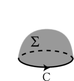
Figure 1: A closed loop $C$ for defining the Wilson loop operator and the surface $\Sigma$ whose boundary is given by the loop $C$.

Now the argument of the exponential is an Abelian quantity, since $A^{g}_{\mu}$ is no longer a matrix, just a number. Therefore, we can apply the (usual) Stokes theorem,

$$\oint_{C=\partial\Sigma}\omega=\int_{\Sigma}d\omega,$$ (9)

to replace the line integral along the closed loop $C$ to the surface integral over the surface $\Sigma$ bounded by $C$. See Fig. 1. Thus we obtain a NAST:

$$W_{C}[\mathscr{A}]=\int[d\mu(g)]_{\Sigma}\exp\left[-ig_{{}_{\rm YM}}\int_{\Sigma:\partial\Sigma=C}F^{g}\right],$$ (10)

where the $F^{g}$ is the curvature two-form defined by

$$F^{g}=dA^{g}=\frac{1}{2}F^{g}_{\mu\nu}(x)dx^{\mu}\wedge dx^{\nu},\quad F^{g}_{\mu\nu}(x):=\partial_{\mu}A_{\nu}^{g}(x)-\partial_{\nu}A_{\mu}^{g}(x),$$ (11)

and the integration measure on the loop $C$ is replaced by the integration measure on the surface $\Sigma$,

$$[d\mu(g)]_{\Sigma}:=\prod_{x\in\Sigma:\partial\Sigma=C}d\mu(g(x)),$$ (12)

by inserting additional integral measures, $1=\int d\mu(g(x))$ for $x\in\Sigma-C$.

The field strength $F^{g}_{\mu\nu}$ is calculated as

$$F^{g}_{\mu\nu}= \partial_{\mu}A_{\nu}^{g}-\partial_{\nu}A_{\mu}^{g}$$

$$= \partial_{\mu}\langle\Lambda|\mathscr{A}_{\nu}^{g}|\Lambda\rangle-\partial_{\nu}\langle\Lambda|\mathscr{A}_{\mu}^{g}|\Lambda\rangle$$

$$= \partial_{\mu}\langle\Lambda|g^{\dagger}\mathscr{A}_{\nu}g|\Lambda\rangle-\partial_{\nu}\langle\Lambda|g^{\dagger}\mathscr{A}_{\mu}g|\Lambda\rangle+ig_{{}_{\rm YM}}^{-1}\partial_{\mu}\langle\Lambda|g^{\dagger}\partial_{\nu}g|\Lambda\rangle-ig_{{}_{\rm YM}}^{-1}\partial_{\nu}\langle\Lambda|g^{\dagger}\partial_{\mu}g|\Lambda\rangle$$

$$= \partial_{\mu}\langle\Lambda|g^{\dagger}\mathscr{A}_{\nu}g|\Lambda\rangle-\partial_{\nu}\langle\Lambda|g^{\dagger}\mathscr{A}_{\mu}g|\Lambda\rangle+ig_{{}_{\rm YM}}^{-1}\langle\Lambda|(\partial_{\mu}g^{\dagger}\partial_{\nu}g-\partial_{\nu}g^{\dagger}\partial_{\mu}g)|\Lambda\rangle+ig_{{}_{\rm YM}}^{-1}\langle\Lambda|g^{\dagger}[\partial_{\mu},\partial_{\nu}]g|\Lambda\rangle$$

$$= \partial_{\mu}\langle\Lambda|g^{\dagger}\mathscr{A}_{\nu}g|\Lambda\rangle-\partial_{\nu}\langle\Lambda|g^{\dagger}\mathscr{A}_{\mu}g|\Lambda\rangle+ig_{{}_{\rm YM}}\langle\Lambda|g^{\dagger}[\Omega_{\mu},\Omega_{\nu}]g|\Lambda\rangle+ig_{{}_{\rm YM}}\langle\Lambda|g^{\dagger}[\partial_{\mu},\partial_{\nu}]g|\Lambda\rangle,$$ (13)

where we have introduced

$$\Omega(x):=ig_{{}_{\rm YM}}^{-1}{g}(x)d{g}^{\dagger}(x).$$ (14)

We define the Lie algebra valued field $m(x)$ which we call the precolor (direction) field by

$$\bm{m}(x):=\left<{\Lambda}|g^{\dagger}(x)T_{A}g(x)|{\Lambda}\right>T_{A}=m^{A}(x)T_{A},\quad{m}^{A}(x)=\left<{\Lambda}|g^{\dagger}(x)T_{A}g(x)|{\Lambda}\right>.$$ (15)

For a Lie algebra valued operator $\mathscr{O}(x)=\mathscr{O}^{A}(x)T_{A}$, we obtain the relation:

$$\langle\Lambda|g^{\dagger}(x)\mathscr{O}(x)g(x)|\Lambda\rangle=\langle\Lambda|g^{\dagger}(x)T_{A}g(x)|\Lambda\rangle\mathscr{O}^{A}(x)=m^{A}(x)\mathscr{O}^{A}(x)=\kappa{\rm tr}(\bm{m}(x)\mathscr{O}(x)),$$ (16)

where we adopted the normalization for the generator:

$${\rm tr}(T_{A}T_{B})=\kappa^{-1}\delta_{AB}.$$ (17)

Therefore, the field strength $F^{g}_{\mu\nu}$ is written as

$$F^{g}_{\mu\nu}(x)= \kappa\{\partial_{\mu}{\rm tr}(\bm{m}(x)\mathscr{A}_{\nu}(x))-\partial_{\nu}{\rm tr}(\bm{m}(x)\mathscr{A}_{\mu}(x))+ig_{{}_{\rm YM}}{\rm tr}(\bm{m}(x)[\Omega_{\mu}(x),\Omega_{\nu}(x)])\}$$

$$+ig_{{}_{\rm YM}}\langle\Lambda|g^{\dagger}(x)[\partial_{\mu},\partial_{\nu}]g(x)|\Lambda\rangle.$$ (18)

Notice that the final term is not gauge invariant and disappears finally after the integration with respect to the gauge-invariant measure $d\mu(g)$. Therefore, it is omitted in what follows.

III Color direction field

As a reference state $\left|{\Lambda}\right>$, we can choose the highest-weight state defined by the (normalized) common eigenvector of the generators $H_{1},H_{2},\cdots,H_{r}$ in the Cartan subalgebra with the eigenvalues $\Lambda_{1},\Lambda_{2},\cdots,\Lambda_{r}$:

$$H_{j}\left|{\Lambda}\right>=\Lambda_{j}\left|{\Lambda}\right>\quad(j=1,\cdots,r),$$ (19)

where $r$ is the rank of $G$, i.e., $r:={\rm rank}G=N-1$. Then we have

$$\left<{\Lambda}|H_{j}|{\Lambda}\right>=\Lambda_{j}\left<{\Lambda}|{\Lambda}\right>=\Lambda_{j}\quad(j=1,\cdots,r),$$ (20)

by taking into account the normalization $\left<{\Lambda}|{\Lambda}\right>=1$.

Let $\mathcal{R}_{+}$ $(\mathcal{R}_{-})$ be a subsystem of positive (negative) roots. Then the highest-weight state satisfies the following properties:

1. $|\Lambda\rangle$ is annihilated by all the (off-diagonal) shift-up operators $E_{\alpha}$ with $\alpha\in\mathcal{R}_{+}$:

   $$E_{\alpha}|\Lambda\rangle=0\quad(\alpha\in\mathcal{R}_{+}),$$ (21)

2. $|\Lambda\rangle$ is annihilated by some shift-down operators $E_{\alpha}$ with $\alpha\in\mathcal{R}_{-}$, not by other $E_{\beta}$ with $\beta\in\mathcal{R}_{-}$:

   $$E_{\alpha}|\Lambda\rangle=0\ ({\rm some~{}}\alpha\in\mathcal{R}_{-});\quad E_{\beta}|\Lambda\rangle=|\Lambda+\beta\rangle\ ({\rm some~{}}\beta\in\mathcal{R}_{-}).$$ (22)

The adjoint rotation of a generator $T_{A}$ can be written as a linear combination of the generators $\{T_{A}\}$:

$$g^{\dagger}(x)T_{A}g(x)= R_{AB}(x)T_{B},$$ (23)

since $g^{\dagger}(x)T_{A}g(x)$ is written by using the commutator repeatedly:

$$g^{\dagger}(x)T_{A}g(x)=e^{iY}T_{A}e^{-iY}=T_{A}+[iY,T_{A}]+\frac{1}{2}[iY,[iY,T_{A}]]+...,\quad Y:=\theta^{B}T_{B},$$ (24)

and the commutator is closed $[T_{A},T_{B}]=if_{ABC}T_{C}$ with the structure constant $f_{ABC}$. Hence, the precolor field (15) is written as

$$\bm{m}(x)=R_{AB}(x)\left<{\Lambda}|T_{B}|{\Lambda}\right>T_{A},\quad{m}^{A}(x)=R_{AB}(x)\left<{\Lambda}|T_{B}|{\Lambda}\right>.$$ (25)

Multiplying $g(x)$ from the left and $g^{\dagger}(x)$ from the right, on the other hand, (23) yields

$$T_{A}= R_{AC}(x)g(x)T_{C}g^{\dagger}(x),$$ (26)

which is cast after multiplying $R_{AB}(x)$ into the form:

$$R_{AB}(x)T_{A}= R_{AB}(x)R_{AC}(x)g(x)T_{C}g^{\dagger}(x)$$

$$= (R^{t})_{BA}(x)R_{AC}(x)g(x)T_{C}g^{\dagger}(x)$$

$$= \bm{1}_{BC}g(x)T_{C}g^{\dagger}(x)$$

$$= g(x)T_{B}g^{\dagger}(x),$$ (27)

where we have used the fact that the matrix $R$ is a real-valued $R_{AB}^{*}=R_{AB}$ and unitary $R^{\dagger}R=RR^{\dagger}=\bm{1}$, in other words, $R$ is an orthogonal matrix satisfying $R^{t}R=RR^{t}=\bm{1}$ for the transposed matrix $R^{t}$ of $R$, because the structure constant is real-valued.

By substituting (27) into (25), the precolor field is written as

$$\bm{m}(x)= \left<{\Lambda}|T_{B}|{\Lambda}\right>g(x)T_{B}g^{\dagger}(x)$$

$$= \left<{\Lambda}|H_{j}|{\Lambda}\right>g(x)H_{j}g^{\dagger}(x)$$

$$= \Lambda_{j}g(x)H_{j}g^{\dagger}(x),$$ (28)

where we have used in the second equality the fact that the generators $T_{A}$ other than the Cartan generators $H_{j}$, i.e., the shift-up and shift-down generators $E_{\alpha}$ in the Cartan basis have the property:

$$\left<{\Lambda}|E_{\alpha}|{\Lambda}\right>=0,$$ (29)

since $E_{\alpha}\left|{\Lambda}\right>=0$ or $E_{\beta}\left|{\Lambda}\right>$ is the eigenvector with the eigenvalue ${\Lambda}+{\beta}$ and obeys

$$\left<{\Lambda}|E_{\beta}|{\Lambda}\right>=N_{\beta,\Lambda}\left<{\Lambda}|{\Lambda}+{\beta}\right>=0,$$ (30)

because the eigenvectors with the different eigenvalues are orthogonal $\left<{\Lambda}|{\Lambda}^{\prime}\right>=0$ for $\Lambda\neq\Lambda^{\prime}$. We have used (20) in the last equality.

We introduce $r$ Lie algebra valued fields $\bm{n}_{j}(x)$ defined by

$$\bm{n}_{j}(x):=g(x)H_{j}g^{\dagger}(x)=n^{A}_{j}(x)T_{A}\quad(j=1,...,r).$$ (31)

Then we arrived at the important relation:

$$\bm{m}(x):=\Lambda_{j}\bm{n}_{j}(x)\in\mathscr{G}=Lie(G)=su(N),\quad m^{A}(x):=\Lambda_{j}n^{A}_{j}(x).$$ (32)

Notice that (23) is determined by the commutation relation alone and, hence, $R_{AB}$ does not depend on the representation adopted. Therefore, $n^{A}_{j}(x)$ does not depend on the representation

$$n^{A}_{j}(x)=R_{Aj}(x),$$ (33)

and we can use the fundamental representation to calculate $n^{A}_{j}(x)$ and to calculate the precolor field $m^{A}(x)$.

$${m}^{A}(x)=\left<{\Lambda}|g^{\dagger}(x)T_{A}g(x)|{\Lambda}\right>=\Lambda_{j}n^{A}_{j}(x)=\Lambda_{j}g(x)H_{j}g^{\dagger}(x).$$ (34)

IV Derivation

We define $\mathscr{B}_{\mu}(x)$ by

$$\mathscr{B}_{\mu}(x):=ig_{{}_{\rm YM}}^{-1}[\bm{n}_{j}(x),\partial_{\mu}\bm{n}_{j}(x)].$$ (35)

In what follows, the summation over $j$ should be understood. Then it satisfies the relation:

$$ig_{{}_{\rm YM}}[\mathscr{B}_{\mu}(x),\bm{n}_{j}(x)]=\partial_{\mu}\bm{n}_{j}(x)\quad(j=1,2,\cdots,r).$$ (36)

The relation (36) is derived in Appendix A. Hence we obtain a relation for the precolor field $\bm{m}(x)=\Lambda_{j}\bm{n}_{j}(x)$:

$$\partial_{\mu}\bm{m}(x)=ig_{{}_{\rm YM}}[\mathscr{B}_{\mu}(x),\bm{m}(x)].$$ (37)

On the other hand, we find

$$\partial_{\mu}\bm{n}_{j}(x)=ig_{{}_{\rm YM}}[\Omega_{\mu},\bm{n}_{j}(x)].$$ (38)

This relation follows from

$$\partial_{\mu}{\bm{n}_{j}}=\partial_{\mu}(gH_{j}g^{\dagger}) =\partial_{\mu}gg^{\dagger}gH_{j}g^{\dagger}+gH_{j}g^{\dagger}g\partial_{\mu}g^{\dagger}$$

$$=-g\partial_{\mu}g^{\dagger}gH_{j}g^{\dagger}+gH_{j}g^{\dagger}g\partial_{\mu}g^{\dagger}$$

$$=-[g\partial_{\mu}g^{\dagger},gH_{j}g^{\dagger}]$$

$$=ig_{{}_{\rm YM}}[\Omega_{\mu},{\bm{n}_{j}}],$$ (39)

where we have used $g^{\dagger}g=\bm{1}=gg^{\dagger}$ in the second equality and $\partial_{\mu}gg^{\dagger}=-g\partial_{\mu}g^{\dagger}$ following from $\partial_{\mu}(gg^{\dagger})=0$ in the third equality. Therefore, we obtain another relation for the precolor field $\bm{m}(x)=\Lambda_{j}\bm{n}_{j}(x)$:

$$\partial_{\mu}\bm{m}(x)=ig_{{}_{\rm YM}}[\Omega_{\mu}(x),\bm{m}(x)],$$ (40)

Combining (37) and (40), we conclude

$$[\Omega_{\mu}(x),\bm{m}(x)]=[\mathscr{B}_{\mu}(x),\bm{m}(x)].$$ (41)

The relation (41) is used to write the third term in $F^{g}_{\mu\nu}(x)$ as

$$ig_{{}_{\rm YM}}{\rm tr}(\bm{m}[\Omega_{\mu},\Omega_{\nu}])=ig_{{}_{\rm YM}}^{-1}{\rm tr}([\partial_{\mu}\bm{n}_{j},\partial_{\nu}\bm{n}_{j}]\bm{m}),$$ (42)

The relation (42) is also derived in Appendix A. Therefore, the field strength $F^{g}_{\mu\nu}$ is written as

$$F^{g}_{\mu\nu}(x)= \kappa(\partial_{\mu}{\rm tr}\{\bm{m}(x)\mathscr{A}_{\nu}(x)\}-\partial_{\nu}{\rm tr}\{\bm{m}(x)\mathscr{A}_{\mu}(x)\}+ig_{{}_{\rm YM}}^{-1}{\rm tr}\{\bm{m}(x)[\partial_{\mu}\bm{n}_{k}(x),\partial_{\nu}\bm{n}_{k}(x)]\}),$$

$$= \partial_{\mu}\{\bm{m}^{A}(x)\mathscr{A}_{\nu}^{A}(x)\}-\partial_{\nu}\{\bm{m}^{A}(x)\mathscr{A}_{\mu}^{A}(x)\}-g_{{}_{\rm YM}}^{-1}f^{ABC}\bm{m}^{A}(x)\partial_{\mu}\bm{n}_{k}^{B}(x)\partial_{\nu}\bm{n}_{k}^{C}(x).$$ (43)

Thus, we have arrived at the final form of the NAST for $SU(N)$ in arbitrary representation:

$$W_{C}[\mathscr{A}]= \int[d\mu(g)]_{\Sigma}\exp\left[-ig_{{}_{\rm YM}}\int_{\Sigma:\partial\Sigma=C}F^{g}\right],\quad F^{g}:=\frac{1}{2}f^{g}_{\mu\nu}(x)dx^{\mu}\wedge dx^{\nu},$$

$$F^{g}_{\mu\nu}(x)= \Lambda_{j}\{\partial_{\mu}[{n}_{j}^{A}(x)\mathscr{A}_{\nu}^{A}(x)]-\partial_{\nu}[{n}_{j}^{A}(x)\mathscr{A}_{\mu}^{A}(x)]-g_{{}_{\rm YM}}^{-1}f^{ABC}{n}_{j}^{A}(x)\partial_{\mu}{n}_{k}^{B}(x)\partial_{\nu}{n}_{k}^{C}(x)\},$$

$$\bm{n}_{j}(x)= g(x)H_{j}g^{\dagger}(x)=n^{A}_{j}(x)T_{A}\quad(j=1,...,r).$$ (44)

We can introduce also the normalized and traceless field $\bm{n}(x)$ which we call the color (direction) field Kondo08 :

$$\bm{n}(x):=\sqrt{\frac{2N}{N-1}}{\bm{m}}(x),\quad\text{or}\quad\bm{m}(x):=\sqrt{\frac{N-1}{2N}}{\bm{n}}(x),$$ (45)

to rewrite the NAST into

$$W_{C}[\mathscr{A}]= \int[d\mu(g)]_{\Sigma}\exp\left[-ig_{{}_{\rm YM}}\sqrt{\frac{N-1}{2N}}\int_{\Sigma:\partial\Sigma=C}f^{g}\right],\quad f^{g}:=\frac{1}{2}f^{g}_{\mu\nu}(x)dx^{\mu}\wedge dx^{\nu},$$

$$f^{g}_{\mu\nu}(x)= \kappa(\partial_{\mu}{\rm tr}\{\bm{n}(x)\mathscr{A}_{\nu}(x)\}-\partial_{\nu}{\rm tr}\{\bm{n}(x)\mathscr{A}_{\mu}(x)\}+ig_{{}_{\rm YM}}^{-1}{\rm tr}\{\bm{n}(x)[\partial_{\mu}\bm{n}_{k}(x),\partial_{\nu}\bm{n}_{k}(x)]\}),$$

$$= \partial_{\mu}\{{n}^{A}(x)\mathscr{A}_{\nu}^{A}(x)\}-\partial_{\nu}\{{n}^{A}(x)\mathscr{A}_{\mu}^{A}(x)\}-g_{{}_{\rm YM}}^{-1}f^{ABC}{n}^{A}(x)\partial_{\mu}{n}_{k}^{B}(x)\partial_{\nu}{n}_{k}^{C}(x),$$

$$\bm{n}(x)= \sqrt{\frac{2N}{N-1}}\Lambda_{j}\bm{n}_{j}(x),\quad\bm{n}_{j}(x)=g(x)H_{j}g^{\dagger}(x)\quad(j=1,...,r).$$ (46)

In what follows, we work out the $G=SU(3)$ case for concreteness. For $G=SU(3)$, we choose the highest-weight state as the reference state. Then the highest-weight vector of the representation with the Dynkin indices $[m,n]$ is given by

$$\vec{\Lambda}=(\Lambda_{3},\Lambda_{8})=\left(\frac{m}{2},\frac{m+2n}{2\sqrt{3}}\right).$$ (47)

The fields $\bm{n}_{3}$ and $\bm{n}_{8}$ are independent of the representation and, hence, can be calculated in the fundamental representation:

$$\bm{n}_{3}(x)=g(x)H_{3}g^{\dagger}(x)=g(x)\frac{\lambda_{3}}{2}g^{\dagger}(x),\quad\bm{n}_{8}(x)=g(x)H_{8}g^{\dagger}(x)=g(x)\frac{\lambda_{8}}{2}g^{\dagger}(x),$$ (48)

with the components:

$${n}_{3}^{A}(x)=2{\rm tr}\left[\frac{\lambda_{A}}{2}g(x)\frac{\lambda_{3}}{2}g^{\dagger}(x)\right],\quad{n}_{8}^{A}(x)=2{\rm tr}\left[\frac{\lambda_{A}}{2}g(x)\frac{\lambda_{8}}{2}g^{\dagger}(x)\right],$$ (49)

where $\lambda_{3}$ and $\lambda_{8}$ are the diagonal matrices of the Gell-Mann matrices $\lambda_{A}$ ($A=1,...,8$) for the Lie algebra $su(3)=Lie(SU(3))$. The parametrization of a group element $g$ and the explicit form of the integration measure $d\mu(g)$ can be found in KT00 .

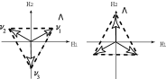
Figure 2: The weight diagram for the fundamental representation of $SU(3)$, (Left) $[1,0]={\bf 3}$, where $\vec{\Lambda}=\vec{h}_{1}=\vec{\nu}_{1}:=(\frac{1}{2},\frac{1}{2\sqrt{3}})$ is the highest weight and the other weights are $\vec{\nu}_{2}:=(-\frac{1}{2},\frac{1}{2\sqrt{3}})$and $\vec{\nu}_{3}:=(0,-\frac{1}{\sqrt{3}})$, (Right) $[0,1]={\bf 3}^{*}$, the highest weight is $-\vec{\nu}_{3}:=(0,\frac{1}{\sqrt{3}})$ and the other weights are $-\vec{\nu}_{2}:=(\frac{1}{2},-\frac{1}{2\sqrt{3}})$ and $-\vec{\nu}_{1}:=(-\frac{1}{2},-\frac{1}{2\sqrt{3}})$.

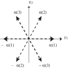
Figure 3: The root diagram of $SU(3)$ is equal to the weight diagram of the adjoint representation $[1,1]={\bf 8}$ of $SU(3)$. Here the positive root vectors are given by $\vec{\alpha}^{(1)}=(1,0)$, $\vec{\alpha}^{(2)}=(\frac{1}{2},\frac{\sqrt{3}}{2})$, and $\vec{\alpha}^{(3)}=(\frac{-1}{2},\frac{\sqrt{3}}{2})$. The two simple roots are given by $\alpha^{1}:=\vec{\alpha}^{(1)}$ and $\alpha^{2}:=\vec{\alpha}^{(3)}$. $\vec{\Lambda}=(\frac{1}{2},\frac{\sqrt{3}}{2})$ is the highest weight of the adjoint representation.

For the fundamental representation $[0,1]$, the color field takes the value in the Lie algebra of $SU(3)/U(2)=CP^{2}$ (See Fig. 2):

$$\bm{m}(x)=\frac{1}{\sqrt{3}}\bm{n}(x)=\frac{1}{\sqrt{3}}\bm{n}_{8}(x)=\frac{1}{\sqrt{3}}g(x)\frac{\lambda_{8}}{2}g^{\dagger}(x)=\frac{1}{6}g(x)\small\begin{pmatrix}1&0&0\cr 0&1&0\cr 0&0&-2\end{pmatrix}g^{\dagger}(x)\in Lie[SU(3)/U(2)].$$ (50)

This is also the case for the fundamental representation $[1,0]$:

$$\bm{m}(x)=\frac{1}{2}\bm{n}_{3}(x)+\frac{1}{2\sqrt{3}}\bm{n}_{8}(x)=g(x)\left[\frac{1}{2}\frac{\lambda_{3}}{2}+\frac{1}{2\sqrt{3}}\frac{\lambda_{8}}{2}\right]g^{\dagger}(x)=\frac{-1}{6}g(x)\small\begin{pmatrix}-2&0&0\cr 0&1&0\cr 0&0&1\end{pmatrix}g^{\dagger}(x)\in Lie[SU(3)/U(2)].$$ (51)

The fundamental representations have the same structure characterized by the degenerate matrix: the two of the three diagonal elements are equal, despite their different appearance.

For the adjoint representation $[1,1]$, on the other hand, the color field takes the value in the Lie algebra of $SU(3)/U(1)^{2}=F^{2}$ (see Fig. 3):

$$\bm{m}(x)=\frac{1}{2}\bm{n}_{3}(x)+\frac{\sqrt{3}}{2}\bm{n}_{8}(x)=g(x)\left[\frac{1}{2}\frac{\lambda_{3}}{2}+\frac{\sqrt{3}}{2}\frac{\lambda_{8}}{2}\right]g^{\dagger}(x)=\frac{1}{2}g(x)\small\begin{pmatrix}1&0&0\cr 0&0&0\cr 0&0&-1\end{pmatrix}g^{\dagger}(x)\in Lie[SU(3)/U(1)^{2}].$$ (52)

Here the matrix between $g$ and $g^{\dagger}$ is not degenerate: the three diagonal elements take different values.

For the general representation with the Dynkin index $[m,n]$, the color field reads

$$\bm{m}(x)=\frac{1}{\sqrt{3}}\bm{n}(x)=\frac{m}{2}\bm{n}_{3}(x)+\frac{m+2n}{2\sqrt{3}}\bm{n}_{8}(x)=\frac{1}{3}g(x)\small\begin{pmatrix}2m+n&0&0\cr 0&-m+n&0\cr 0&0&-m-2n\end{pmatrix}g^{\dagger}(x)\in Lie[SU(3)/\tilde{H}].$$ (53)

where $\tilde{H}$ is called the maximal stability subgroup.

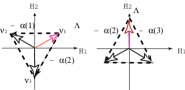
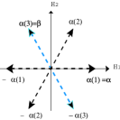
Figure 4: The relationships among the weight vectors $\vec{\nu}_{1},\vec{\nu}_{2},\vec{\nu}_{3}$ in the fundamental representations ${\bf 3}$ and the root vectors $\vec{\alpha}^{(1)},\vec{\alpha}^{(2)},\vec{\alpha}^{(3)}$ in $SU(3)$. We find $\vec{\nu}_{1}\perp\vec{\alpha}^{(3)},-\vec{\alpha}^{(3)}$. Here $\vec{\Lambda}=\vec{\nu}_{1}:=(\frac{1}{2},\frac{1}{2\sqrt{3}})$ is the highest weight of the fundamental representation ${\bf 3}$.

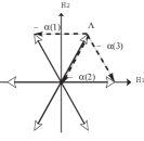
Figure 5: The weight vectors and root vectors required to define the coherent state in the adjoint representation $[1,1]={\bf 8}$ of $SU(3)$, where $\vec{\Lambda}=(\frac{1}{2},\frac{\sqrt{3}}{2})$ is the highest weight of the adjoint representation.

Thus,we can show that every representation $R$ of $SU(3)$ specified by the Dynkin index $[m,n]$ belongs to (I) or (II):

1. Minimal case: If $mn=0$ ($m=0$ or $n=0$), the maximal stability group $\tilde{H}$ is given by

   $$\tilde{H}=U(2),$$ (54)

   with generators $\{H_{1},H_{2},E_{\beta},E_{-\beta}\}$. In the minimal case, ${\rm dim}(G/\tilde{H})$ is minimal. Such a degenerate case occurs when the highest-weight vector $\vec{\Lambda}$ is orthogonal to some root vectors. In the minimal case, the coset $G/\tilde{H}$ is given by the complex projective space:

   $$G/\tilde{H}=SU(3)/U(2)=SU(3)/(SU(2)\times U(1))=CP^{2},$$ (55)

   For example, the fundamental representation $[1,0]$ has the maximal stability subgroup $U(2)$ with the generators $\{H_{1},H_{2},E_{\alpha^{(3)}},E_{-\alpha^{(3)}}\}\in u(2)$, where

   $$\vec{\Lambda}=\vec{\nu}_{1}\perp\vec{\alpha}^{(3)},-\vec{\alpha}^{(3)}.$$ (56)

   See Fig. 4.

2. Maximal case: If $mn\not=0$ ($m\not=0$ and $n\not=0$), $\tilde{H}$ is the maximal torus group:

   $$\tilde{H}=H=U(1)\times U(1),$$ (57)

   with generators $\{H_{1},H_{2}\}$. In the maximal case, ${\rm dim}(G/\tilde{H})$ is maximal. This is a non-degenerate case. In the maximal case, the coset $G/\tilde{H}$ is given by the flag space:

   $$G/\tilde{H}=SU(3)/(U(1)\times U(1))=F_{2}.$$ (58)

   For example, the adjoint representation $[1,1]$ has the maximal stability subgroup $U(1)\times U(1)$ with the generators $\{H_{1},H_{2}\}\in u(1)+u(1)$. See Fig.5.

V Magnetic monopoles

We can define the gauge-invariant magnetic-monopole current $k=\delta{}^{*}f^{g}$ from the field strength $f^{g}_{\mu\nu}$ through the NAST. The magnetic–monopole current $k$ is defined as the ($D-3$)-form using the gauge-invariant field strength (curvature two-form) by

$$k=\delta{}^{\displaystyle*}f^{g}={}^{\displaystyle*}df^{g},\quad f^{g}=\sum_{j=1}^{r}\Lambda_{j}f^{(j)}.$$ (59)

Using the same procedure as given in Kondo08 , the Wilson loop operator in arbitrary representation of $SU(N)$ is written in terms of the electric current $j$ and the magnetic current $k$:

$$W_{C}[\mathscr{A}]=\int[d\mu({g})]\exp\left\{-ig_{{}_{\rm YM}}\sqrt{\frac{N-1}{2N}}[(\omega_{\Sigma_{C}},k)+(N_{\Sigma_{C}},j)]\right\},$$ (60)

where we have defined the $(D-3)$-form $k$ and the one-form $j$ in $D$ spacetime dimensions:

$$k:=\delta{}^{\displaystyle*}f^{g},\quad j:= \delta f^{g},$$ (61)

we have introduced an antisymmetric tensor $\Theta_{\Sigma_{C}}$ of rank two which has the support only on the surface $\Sigma_{C}$ spanned by the loop $C$:

$$\Theta^{\mu\nu}_{\Sigma_{C}}(x):=\int_{\Sigma_{C}:\partial\Sigma_{C}=C}d^{2}S^{\mu\nu}(x(\sigma))\delta^{D}(x-x(\sigma)),$$ (62)

and we have defined the $(D-3)$-form $\omega_{\Sigma_{C}}$ and one-form $N_{\Sigma_{C}}$ using the Laplacian $\Delta$ by

$$\omega_{\Sigma_{C}}:={}^{\displaystyle*}d\Delta^{-1}\Theta_{\Sigma_{C}}=\delta\Delta^{-1}{}^{\displaystyle*}\Theta_{\Sigma_{C}},\quad N_{\Sigma_{C}}:=\delta\Delta^{-1}\Theta_{\Sigma_{C}},$$ (63)

with the inner product for two forms being defined by

$$(\omega_{\Sigma_{C}},k)=\frac{1}{(D-3)!}\int d^{D}xk^{\mu_{1}\cdots\mu_{D-3}}(x)\omega^{\mu_{1}\cdots\mu_{D-3}}_{\Sigma_{C}}(x),$$

$$(N_{\Sigma_{C}},j)=\int d^{D}xj^{\mu}(x)N^{\mu}_{\Sigma_{C}}(x).$$ (64)

Here we have replaced the measure $[d\mu({g})]_{\Sigma}$ by $[d\mu({g})]:=[d\mu({g})]_{\mathbb{R}^{D}}=\prod_{x\in\mathbb{R}^{D}}d\mu({g}(x))$ over all the spacetime points.

For $D=4$, especially, the magnetic current reads

$$k^{\mu}=\frac{1}{2}\epsilon^{\mu\nu\rho\sigma}\partial_{\nu}f_{\rho\sigma}^{g},\quad f_{\mu\nu}^{g}=\sum_{j=1}^{r}\Lambda_{j}f^{(j)}_{\mu\nu}.$$ (65)

Then, the magnetic charge is defined by

$$q_{m}=\int d^{3}xk^{0}=\int d^{3}x\frac{1}{2}\epsilon^{jk\ell}\partial_{\ell}f_{jk}^{g}(x)=\int d^{2}S_{\ell}\epsilon^{jk\ell}\frac{1}{2}f_{jk}^{g}(x).$$ (66)

We examine the quantization condition for the magnetic charge. In the $SU(3)$ case, the two kinds of gauge-invariant field strength are given by

$$f_{\mu\nu}^{g}= \Lambda_{1}f_{\mu\nu}^{(1)}+\Lambda_{2}f_{\mu\nu}^{(2)},$$

$$f_{\mu\nu}^{(1)}= \partial_{\mu}2{\rm tr}\{\bm{n}_{3}\mathscr{A}_{\nu}\}-\partial_{\nu}2{\rm tr}\{\bm{n}_{3}\mathscr{A}_{\mu}\}-ig_{{}_{\rm YM}}^{-1}2{\rm tr}\{\bm{n}_{3}[\partial_{\mu}\bm{n}_{3},\partial_{\nu}\bm{n}_{3}]+\bm{n}_{3}[\partial_{\mu}\bm{n}_{8},\partial_{\nu}\bm{n}_{8}]\},$$

$$f_{\mu\nu}^{(2)}= \partial_{\mu}2{\rm tr}\{\bm{n}_{8}\mathscr{A}_{\nu}\}-\partial_{\nu}2{\rm tr}\{\bm{n}_{8}\mathscr{A}_{\mu}\}-ig_{{}_{\rm YM}}^{-1}2{\rm tr}\{\bm{n}_{8}[\partial_{\mu}\bm{n}_{3},\partial_{\nu}\bm{n}_{3}]+\bm{n}_{8}[\partial_{\mu}\bm{n}_{8},\partial_{\nu}\bm{n}_{8}]\}$$

$$= \partial_{\mu}2{\rm tr}\{\bm{n}_{8}\mathscr{A}_{\nu}\}-\partial_{\nu}2{\rm tr}\{\bm{n}_{8}\mathscr{A}_{\mu}\}-\frac{4}{3}ig_{{}_{\rm YM}}^{-1}2{\rm tr}\{\bm{n}_{8}[\partial_{\mu}\bm{n}_{8},\partial_{\nu}\bm{n}_{8}]).$$ (67)

Notice that $f_{\mu\nu}^{(2)}$ is written in terms of $\bm{n}_{8}$ alone (see Appendix B for the derivation of $f_{\mu\nu}^{(2)}$). It is shown KKSS15 that the two kinds of the gauge-invariant charges $q_{m}^{(1)}$ and $q_{m}^{(2)}$ obey the different quantization conditions:

$$q_{m}= \Lambda_{1}q_{m}^{(1)}+\Lambda_{2}q_{m}^{(2)},$$

$$q_{m}^{(1)}:= \int d^{3}x\frac{1}{2}\epsilon^{jk\ell}\partial_{\ell}f_{jk}^{(1)}(x)=\frac{4\pi}{g_{{}_{\rm YM}}}\left(n-\frac{1}{2}n^{\prime}\right),$$

$$q_{m}^{(2)}:= \int d^{3}x\frac{1}{2}\epsilon^{jk\ell}\partial_{\ell}f_{jk}^{(2)}(x)=\frac{4\pi}{g_{{}_{\rm YM}}}\frac{1}{2}\sqrt{3}n^{\prime},\quad n,n^{\prime}\in\mathbb{Z}.$$ (68)

The existence of the magnetic charge $q_{m}^{(1)}$ characterized by two integers $n$ and $n^{\prime}$ is consistent with a fact that the map defined by

$$\bm{n}_{3}:S^{2}\rightarrow SU(3)/[U(1)\times U(1)]\simeq F_{2},$$ (69)

has the nontrivial Homotopy group:

$$\pi_{2}(SU(3)/[U(1)\times U(1)])=\pi_{1}(U(1)\times U(1))=\mathbb{Z}+\mathbb{Z}.$$ (70)

On the other hand, the existence of the magnetic charge $q_{m}^{(2)}$ characterized by an integer $n^{\prime}$ is consistent with a fact that the map defined by

$$\bm{n}_{8}:S^{2}\rightarrow SU(3)/U(2)\simeq\mathbb{C}P^{2},$$ (71)

has the following nontrivial homotopy group:

$$\pi_{2}(SU(3)/[SU(2)\times U(1)])=\pi_{1}(SU(2)\times U(1))=\pi_{1}(U(1))=\mathbb{Z}.$$ (72)

Incidentally, we can show KKSS15 that the gauge-invariant field strength $F^{g}_{\mu\nu}$ is equal to the component of the non-Abelian field strength $\mathscr{F}[\mathscr{V}]$ of the restricted field $\mathscr{V}$ (in the decomposition $\mathscr{A}=\mathscr{V}+\mathscr{X}$) projected to the color field $\bm{n}$:

$$F^{g}_{\mu\nu}={\rm tr}\{\bm{m}\mathscr{F}_{\mu\nu}[\mathscr{V}]\}=\Lambda_{j}f_{\mu\nu}^{(j)},\quad f_{\mu\nu}^{(j)}={\rm tr}\{\bm{n}_{j}\mathscr{F}[\mathscr{V}]\}.$$ (73)

This relation is useful in calculating the contribution from magnetic monopoles to the Wilson loop average from the viewpoint of the dual superconductor picture for quark confinement. The results will be given elsewhere.

Acknowledgements —

The authors would like to thank Toru Shinohara for discussions on the field strength for the magnetic monopole. This work is supported by Grants-in-Aid for Scientific Research (C) No.24540252 and (C) No.15K05042 from the Japan Society for the Promotion of Science (JSPS).

Appendix A Derivation of eq.(36) and eq.(42)

Equation (36) is derived as follows.

$$ig_{{}_{\rm YM}}[\mathscr{B}_{\mu},\bm{n}_{j}]= -[[\bm{n}_{k},\partial_{\mu}\bm{n}_{k}],\bm{n}_{j}]$$

$$= [[\partial_{\mu}\bm{n}_{k},\bm{n}_{j}],\bm{n}_{k}]+[[\bm{n}_{j},\bm{n}_{k}],\partial_{\mu}\bm{n}_{k}]$$

$$= [[\partial_{\mu}\bm{n}_{j},\bm{n}_{k}],\bm{n}_{k}]$$

$$= [\bm{n}_{k},[\bm{n}_{k},\partial_{\mu}\bm{n}_{j}]]$$

$$= \partial_{\mu}\bm{n}_{j}-\bm{n}_{k}(\bm{n}_{k},\partial_{\mu}\bm{n}_{j}).$$ (74)

where we have used the Jacobi identity in the second equality, the relation $[\partial_{\mu}\bm{n}_{k},\bm{n}_{j}]=[\partial_{\mu}\bm{n}_{j},\bm{n}_{k}]$ following from $\partial_{\mu}[\bm{n}_{k},\bm{n}_{j}]=0$ and the commutativity $[\bm{n}_{j},\bm{n}_{k}]=0$ in the third equality, and the identity $\mathscr{F}=\bm{n}_{k}(\bm{n}_{k},\mathscr{F})+[\bm{n}_{k},[\bm{n}_{k},\mathscr{F}]]$ (see e.g., Appendix C of KKSS15 ) in the fifth equality. Moreover, we find that the last term in (74) vanishes:

$$(\bm{n}_{k},\partial_{\mu}\bm{n}_{j})= \kappa{\rm tr}(\bm{n}_{k}\partial_{\mu}\bm{n}_{j})$$

$$= \kappa{\rm tr}(gH_{k}g^{\dagger}\partial_{\mu}(gH_{j}g^{\dagger}))$$

$$= \kappa{\rm tr}(gH_{k}g^{\dagger}\partial_{\mu}gH_{j}g^{\dagger})+\kappa{\rm tr}(gH_{k}g^{\dagger}gH_{j}\partial_{\mu}g^{\dagger})$$

$$= -\kappa{\rm tr}(gH_{k}\partial_{\mu}g^{\dagger}gH_{j}g^{\dagger})+\kappa{\rm tr}(gH_{k}H_{j}\partial_{\mu}g^{\dagger})$$

$$= -\kappa{\rm tr}(gH_{j}g^{\dagger}gH_{k}\partial_{\mu}g^{\dagger})+\kappa{\rm tr}(gH_{k}H_{j}\partial_{\mu}g^{\dagger})$$

$$= -\kappa{\rm tr}(gH_{j}H_{k}\partial_{\mu}g^{\dagger})+\kappa{\rm tr}(gH_{k}H_{j}\partial_{\mu}g^{\dagger})$$

$$= \kappa{\rm tr}(g[H_{k},H_{j}]\partial_{\mu}g^{\dagger})=0,$$ (75)

where we have used $g^{\dagger}g=\bm{1}=gg^{\dagger}$ and $g^{\dagger}\partial_{\mu}g=-\partial_{\mu}g^{\dagger}g$ following from $\partial_{\mu}(gg^{\dagger})=0$ in the fourth equality and cyclicity of the trace in the fifth equality. Combining (74) and (75), indeed, we have (36).

Equation (42) is derived as follows. The third term in $F^{g}_{\mu\nu}(x)$ is rewritten using the relation (41) as

$$ig_{{}_{\rm YM}}{\rm tr}(\bm{m}[\Omega_{\mu},\Omega_{\nu}])= ig_{{}_{\rm YM}}{\rm tr}([\bm{m},\Omega_{\mu}]\Omega_{\nu})$$

$$= ig_{{}_{\rm YM}}{\rm tr}(\Omega_{\nu}[\bm{m},\mathscr{B}_{\mu}])$$

$$= ig_{{}_{\rm YM}}{\rm tr}([\Omega_{\nu},\bm{m}]\mathscr{B}_{\mu})$$

$$= ig_{{}_{\rm YM}}{\rm tr}([\mathscr{B}_{\nu},\bm{m}]\mathscr{B}_{\mu})$$

$$= {\rm tr}(\partial_{\nu}\bm{m}\mathscr{B}_{\mu})$$

$$= ig_{{}_{\rm YM}}^{-1}{\rm tr}(\partial_{\nu}\bm{m}[\bm{n}_{j},\partial_{\mu}\bm{n}_{j}])$$

$$= ig_{{}_{\rm YM}}^{-1}{\rm tr}([\partial_{\nu}\bm{m},\bm{n}_{j}]\partial_{\mu}\bm{n}_{j})$$

$$= ig_{{}_{\rm YM}}^{-1}{\rm tr}([\partial_{\nu}\bm{n}_{j},\bm{m}]\partial_{\mu}\bm{n}_{j})$$

$$= ig_{{}_{\rm YM}}^{-1}{\rm tr}([\partial_{\mu}\bm{n}_{j},\partial_{\nu}\bm{n}_{j}]\bm{m}),$$ (76)

where we have used ${\rm tr}\{A[B,C]\}={\rm tr}\{[A,B]C\}={\rm tr}\{B[C,A]\}={\rm tr}\{C[A,B]\}$ due to the cyclicity of the trace in the first, third, and seventh equalities, and the relation $[\partial_{\nu}\bm{m},\bm{n}_{j}]=[\partial_{\nu}\bm{n}_{j},\bm{m}]$ which is derived from $\partial_{\nu}[\bm{m},\bm{n}_{j}]=0$ and the commutativity $[\bm{m},\bm{n}_{j}]=0$ in the eighth equality.

Appendix B Field strength for the magnetic monopole

For $G=SU(N)$, we can define three types of products: $\cdot$, $\times$, and $*$ in the vector form by

$$\mathbf{X}\cdot\mathbf{Y}:= X^{A}Y^{A}=\mathbf{Y}\cdot\mathbf{X},$$ (77a)

$$(\mathbf{X}\times\mathbf{Y})^{C}:= f_{ABC}X^{A}Y^{B}=-(\mathbf{Y}\times\mathbf{X})^{C},$$ (77b)

$$(\mathbf{X}*\mathbf{Y})^{C}:= d_{ABC}X^{A}Y^{B}=(\mathbf{Y}*\mathbf{X})^{C},$$ (77c)

which correspond to three operations in the Lie algebra form: ${\rm tr}()$, $[,]$, and $\{,\}$ as

$$2{\rm tr}(\mathscr{X}\mathscr{Y})= \mathscr{X}^{A}\mathscr{Y}^{A},$$ (78a)

$$[\mathscr{X},\mathscr{Y}]= if_{ABC}\mathscr{X}^{A}\mathscr{Y}^{B}T_{C},$$ (78b)

$$\{\mathscr{X},\mathscr{Y}\}-\frac{1}{N}2{\rm tr}(\mathscr{X}\mathscr{Y})\mathbf{1}= d_{ABC}\mathscr{X}^{A}\mathscr{Y}^{B}T_{C}.$$ (78c)

Then we obtain the relation:

$$\mathbf{n}_{8}\cdot(\partial_{\mu}\mathbf{n}_{8}\times\partial_{\nu}\mathbf{n}_{8})= \partial_{\nu}\mathbf{n}_{8}\cdot(\mathbf{n}_{8}\times\partial_{\mu}\mathbf{n}_{8})$$

$$= (2\sqrt{3}\mathbf{n}_{3}*\partial_{\nu}\mathbf{n}_{3})\cdot(\mathbf{n}_{8}\times\partial_{\mu}\mathbf{n}_{8})$$

$$= 2\sqrt{3}\partial_{\nu}\mathbf{n}_{3}\cdot[\mathbf{n}_{3}*(\mathbf{n}_{8}\times\partial_{\mu}\mathbf{n}_{8})]$$

$$= 2\sqrt{3}\partial_{\nu}\mathbf{n}_{3}\cdot[\frac{\sqrt{3}}{2}(\mathbf{n}_{8}\times\partial_{\mu}\mathbf{n}_{3})]$$

$$= 3\mathbf{n}_{8}\cdot(\partial_{\mu}\mathbf{n}_{3}\times\partial_{\nu}\mathbf{n}_{3}),$$ (79)

where we have used the identity: $\bm{X}\cdot(\bm{Y}\times\bm{Z})=\bm{Y}\cdot(\bm{Z}\times\bm{X})=\bm{Z}\cdot(\bm{X}\times\bm{Y})$ in the first and the fifth equalities, $\sqrt{3}\mathbf{n}_{3}*\mathbf{n}_{3}=\mathbf{n}_{8}$ in the second equality, and $(\bm{X}*\bm{Y})\cdot\bm{Z}=(\bm{X}*\bm{Z})\cdot\bm{Y}$ in the third equality. The fourth equality is shown as

$$\mathbf{n}_{3}*(\mathbf{n}_{8}\times\partial_{\mu}\mathbf{n}_{8})= \mathbf{n}_{8}\times(\mathbf{n}_{3}*\partial_{\mu}\mathbf{n}_{8})$$

$$= \mathbf{n}_{8}\times(\partial_{\mu}(\mathbf{n}_{3}*\mathbf{n}_{8})-\partial_{\mu}\mathbf{n}_{3}*\mathbf{n}_{8})$$

$$= \frac{1}{\sqrt{3}}\mathbf{n}_{8}\times\partial_{\mu}\mathbf{n}_{3}-\mathbf{n}_{8}\times(\mathbf{n}_{8}*\partial_{\mu}\mathbf{n}_{3})$$

$$= \frac{1}{\sqrt{3}}\mathbf{n}_{8}\times\partial_{\mu}\mathbf{n}_{3}+\frac{1}{2\sqrt{3}}\mathbf{n}_{8}\times\partial_{\mu}\mathbf{n}_{3}$$

$$= \frac{\sqrt{3}}{2}(\mathbf{n}_{8}\times\partial_{\mu}\mathbf{n}_{3}).$$ (80)

where we have used $\bm{X}*(\bm{Y}\times\bm{Z})=\bm{Y}\times(\bm{X}*\bm{Z})+\bm{Z}*(\bm{X}\times\bm{Y})$ and $\mathbf{n}_{3}\times\mathbf{n}_{8}=0$ in the first equality, the Leibniz rule in the second equality, $\sqrt{3}\mathbf{n}_{3}*\mathbf{n}_{8}=\mathbf{n}_{3}$ in the third equality, and $\bm{X}\times(\bm{X}*\bm{Z})=\frac{1}{2}(\bm{X}*\bm{X})\times\bm{Z}$ following from $\bm{X}\times(\bm{Y}*\bm{Z})=(\bm{X}*\bm{Y})\times\bm{Z}+(\bm{X}*\bm{Z})\times\bm{Y}$ and $\sqrt{3}\mathbf{n}_{8}*\mathbf{n}_{8}=-\mathbf{n}_{8}$ in the fourth equality.

This relation was used to write $f_{\mu\nu}^{(2)}$ in the form given in (67):

$$\mathbf{n}_{8}\cdot(\partial_{\mu}\mathbf{n}_{3}\times\partial_{\nu}\mathbf{n}_{3})+\mathbf{n}_{8}\cdot(\partial_{\mu}\mathbf{n}_{8}\times\partial_{\nu}\mathbf{n}_{8})=\frac{4}{3}\mathbf{n}_{8}\cdot(\partial_{\mu}\mathbf{n}_{8}\times\partial_{\nu}\mathbf{n}_{8}).$$ (81)

References

(1)
K. Wilson,
Phys. Rev. D10, 2445–2459
(1974).
(2)
K.-I. Kondo, S. Kato, A. Shibata and T. Shinohara,
Phys. Rep. 579, 1–226 (2015).
arXiv:1409.1599 [hep-th].
(3)
Y. Nambu,
Phys. Rev. D10, 4262–4268 (1974).
G. ’t Hooft,
in: High Energy Physics, edited by A. Zichichi
(Editorice Compositori, Bologna, 1975).
S. Mandelstam,
Phys. Report23, 245–249 (1976).
A.M. Polyakov,
Phys. Lett. B59, 82–84 (1975).
Nucl. Phys. B120, 429–458 (1977).
(4)
D.I. Diakonov and V.Yu. Petrov,
Phys. Lett. B 224, 131–135 (1989).
(5)
D. Diakonov and V. Petrov,
arXiv:hep-th/9606104;
D. Diakonov and V. Petrov,
arXiv:hep-lat/0008004;
D. Diakonov and V. Petrov,
arXiv:hep-th/0008035.
(6)
K.-I. Kondo,
Phys. Rev. D 58, 105016 (1998).
arXiv:hep-th/9805153.
(7)
K.-I. Kondo and Y. Taira,
Mod. Phys. Lett. A 15, 367–377 (2000);
arXiv:hep-th/9906129.
(8)
K.-I. Kondo and Y. Taira,
Prog. Theor. Phys. 104, 1189–1265 (2000).
arXiv:hep-th/9911242.