An FPT 2-Approximation for
Tree-Cut Decomposition

Abstract

The tree-cut width of a graph is a graph parameter defined by Wollan [J. Comb. Theory, Ser. B, 110:47–66, 2015] with the help of tree-cut decompositions. In certain cases, tree-cut width appears to be more adequate than treewidth as an invariant that, when bounded, can accelerate the resolution of intractable problems. While designing algorithms for problems with bounded tree-cut width, it is important to have a parametrically tractable way to compute the exact value of this parameter or, at least, some constant approximation of it. In this paper we give a parameterized $2$-approximation algorithm for the computation of tree-cut width; for an input $n$-vertex graph $G$ and an integer $w$, our algorithm either confirms that the tree-cut width of $G$ is more than $w$ or returns a tree-cut decomposition of $G$ certifying that its tree-cut width is at most $2w$, in time $2^{O(w^{2}\log w)}\cdot n^{2}$. Prior to this work, no constructive parameterized algorithms, even approximated ones, existed for computing the tree-cut width of a graph. As a consequence of the Graph Minors series by Robertson and Seymour, only the existence of a decision algorithm was known.

Keywords: Fixed-Parameter Tractable algorithm; tree-cut width; approximation algorithm.

1 Introduction

One of the most popular ways to decompose a graph into smaller pieces is given by the notion of a tree decomposition. Intuitively, a graph $G$ has a tree decomposition of small width if it can be decomposed into small (possibly overlapping) pieces that are altogether arranged in a tree-like structure. The width of such a decomposition is defined as the minimum size of these pieces. The graph invariant of treewidth corresponds to the minimum width of all possible tree decompositions and, that way, serves as a measure of the topological resemblance of a graph to the structure of a tree. The importance of tree decompositions and treewidth in graph algorithms resides in the fact that a wide family of ${\sf{\sf NP}}$-hard graph problems admits FPT-algorithms, i.e., algorithms that run in $f(w)\cdot n^{O(1)}$ steps, when parameterized by the treewidth $w$ of their input graph. According to the celebrated theorem of Courcelle, for every problem that can be expressed in Monadic Second Order Logic (MSOL) [5] it is possible to design an $f(w)\cdot n$-step algorithm on graphs of treewidth at most $w$. Moreover, towards improving the parametric dependence, i.e., the function $f$, of this algorithm for specific problems, it is possible to design tailor-made dynamic programming algorithms on the corresponding tree decompositions. Treewidth has also been important from the combinatorial point of view. This is mostly due to the celebrated “planar graph exclusion theorem” [14, 15]. This theorem asserts that:

(*) Every graph that does not contain some fixed wall as a topological minor has bounded treewidth.

The above result had a considerable algorithmic impact as every problem for which a negative (or positive) answer can be certified by the existence of some sufficiently big wall in its input, is reduced to its resolution on graphs of bounded treewidth. This induced a lot of research on the derivation of fast parameterized algorithms that can construct (optimally or approximately) these decompositions. For instance, according to [1], treewidth can be computed in $f(OPT)\cdot n$ steps where $f(w)=2^{O(w^{3})}$ while, more recently, a 5-approximation for treewidth was given in [2] that runs in $2^{O(OPT)}\cdot n$ steps.

Unfortunately, the aforementioned success stories about treewidth have some natural limitations. In fact, it is not always possible to use treewidth for improving the tractability of NP-hard problems. In particular, there are interesting cases of problems where no such an FPT-algorithm is expected to exist [7, 10, 6]. Therefore, it is an interesting question whether there are alternative, but still general, graph invariants that can provide tractable parameterizations for such problems.

A promising candidate in this direction is the graph invariant of tree-cut width that was recently introduced by Wollan in [23]. Tree-cut width can be seen as an “edge” analogue of treewidth. It is defined using a different type of decompositions, namely, tree-cut decompositions that are roughly tree-like partitions of a graph into mutually disjoint pieces such that both the size of some “essential” extension of these pieces and the number of edges crossing two neighboring pieces are bounded (see Section 2 for the formal definition). Our first result is that it is NP-hard to decide, given a graph $G$ and an integer $w$, whether the input graph $G$ has tree-cut width at most $w$. This follows from a reduction from the Min Bisection problem that is presented in Subsection 2.2. This encourages us to consider a parameterized algorithm for this problem.

Figure 1: The relations between classes with bounded treewidth (${\bf tw}$) and tree-cut width (${\bf tcw}$).

Another tree-like parameter that can be seen as an edge-counterpart of treewidth is carving-width, defined in [18]. It is known that a graph has bounded carving-width if and only if both its treewidth and its maximum degree are bounded. We stress that this is not the case for tree-cut width, which can also capture graphs with unbounded maximum degree and, thus, is more general than carving-width. There are two reasons why tree-cut width might be a good alternative for treewidth. We expose them below.

(1) Tree-cut width as a parameter. From now on we denote by $\mbox{\bf tcw}(G)$ (resp. $\mathbf{tw}(G)$) the tree-cut width (resp. treewidth) of a graph $G$. As it is shown in [23] $\mbox{\bf tcw}(G)=O(\mathbf{tw}(G)\cdot\Delta(G))$. Moreover, in [8], it was proven that $\mathbf{tw}(G)=O((\mbox{\bf tcw}(G))^{2})$ and in Subsection 2.3, we prove that the latter upper bound is asymptotically tight. The graph class inclusions generated by the aforementioned relations are depicted in Fig. 1. As tree-cut width is a “larger” parameter than treewidth, one may expect that some problems that are intractable when parameterized by treewidth (known to be W$[1]$-hard or open) become tractable when parameterized by tree-cut width. Indeed, some recent progress on the development of a dynamic programming framework for tree-cut width (see [8]) confirms that assumption. According to [8], such problems include Capacitated Dominating Set problem, Capacitated Vertex Cover [6], and Balanced Vertex-Ordering problem. We expect that more problems will fall into this category.

(2) Combinatorics of tree-cut width. In [23] Wollan proved the following counterpart of (*):

(**) Every graph that does not contain some fixed wall as an immersion has bounded tree-cut width.

Notice that (*) yields (**) if we replace “topological minor” by “immersion” and “treewidth” by “tree-cut width”. This implies that tree-cut width has combinatorial properties analogous to those of treewidth. It follows that every problem where a negative (or positive) answer can be certified by the existence of a wall as an immersion, can be reduced to the design of a suitable dynamic programming algorithm for this problem on graphs of bounded tree-cut width.

Computing tree-cut width.

It follows that designing dynamic programming algorithms on tree-cut decompositions might be a promising task when this is not possible (or promising) on tree-decompositions. Clearly, this makes it imperative to have an efficient algorithm that, given a graph $G$ and an integer $w$, constructs tree-cut decompositions of width at most $w$ or reports that this is not possible. Interestingly, an $f(w)\cdot n^{3}$-time algorithm for the decision version of the problem is known to exist but this is not done in a constructive way. Indeed, for every fixed $w$, the class of graphs with tree-cut width at most $w$ is closed under immersions [23]. By the fact that graphs are well-quasi-ordered under immersions [16], for every $w$, there exists a finite set ${\cal R}_{w}$ of graphs such that $G$ has tree-cut width at most $w$ if and only if it does not contain any of the graphs in ${\cal R}_{w}$ as an immersion. From [11], checking whether an $h$-vertex graph $H$ is contained as an immersion in some $n$-vertex graph $G$ can be done in $f(w)\cdot n^{3}$ steps. It follows that, for every fixed $w$, there exists a polynomial algorithm checking whether the tree-cut width of a graph is at most $w$. Unfortunately, the construction of this algorithm requires the knowledge of the set ${\cal R}_{w}$ for every $w$, which is not provided by the results in [16]. Even if we knew ${\cal R}_{w}$, it is not clear how to construct a tree-cut decomposition of width at most $w$, if one exists.

In this paper we make a first step towards a constructive parameterized algorithm for tree-cut width by giving an FPT 2-approximation for it. Given a graph $G$ and an integer $w$, our algorithm either reports that $G$ has tree-cut width more than $w$ or outputs a tree-cut decomposition of width at most $2w$ in $2^{O(w^{2}\log w)}n^{2}$ steps. The algorithm is presented in Section 3.

2 Problem definition and preliminary results

Unless specified otherwise, every graph in this paper is undirected and loopless and may have multiple edges. By $V(G)$ and $E(G)$ we denote the vertex set and the edge set, respectively, of a graph $G$. Given a vertex $x\in V(G)$, the neighborhood of $x$ is $N(x)=\{y\in V(G)\mid xy\in E(G)\}$. Given two disjoint sets $X$ and $Y$ of $V(G)$, we denote $\delta_{G}(X,Y)=\{xy\in E(G)\mid x\in X,y\in Y\}$. For a subset $X$ of $V(G)$, we define $\partial_{G}(X)=\{x\in X\mid N(x)\setminus X\neq\emptyset\}$.

2.1 Tree-cut width and treewidth

Tree-cut width. A tree-cut decomposition of $G$ is a pair $(T,\cal{X})$ where $T$ is a tree and ${\cal X}=\{X_{t}\subseteq V(G)\mid t\in V(T)\}$ such that

• $X_{t}\cap X_{t^{\prime}}=\emptyset$ for all distinct $t$ and $t^{\prime}$ in $V(T)$,

• $\bigcup_{t\in V(T)}X_{t}=V(G)$.

From now on we refer to the vertices of $T$ as nodes. The sets in $\cal{X}$ are called the bags of the tree-cut decomposition. Observe that the conditions above allow to assign an empty bag for some node of $T$. Such nodes are called trivial nodes. Observe that we can always assume that trivial nodes are internal nodes.

Let $L(T)$ be the set of leaf nodes of $T$. For every tree-edge $e=\{u,v\}$ of $E(T)$, we let $T_{u}$ and $T_{v}$ be the subtrees of $T\setminus e$ which contain $u$ and $v$, respectively.

We define the adhesion of a tree-edge $e=\{u,v\}$ of $T$ as follows:

$$\delta^{T}(e)=\delta_{G}(\bigcup_{t\in V(T_{u})}X_{t},\bigcup_{t\in V(T_{v})}X_{t}).$$

For a graph $G$ and a set $X\subseteq V(G)$, the 3-center of $(G,X)$ is the graph obtained from $G$ by repetitively dissolving every vertex $v\in V(G)\setminus X$ that has two neighbors and degree 2 and removing every vertex $w\in V(G)\setminus X$ that has degree at most 2 and one neighbor (dissolving a vertex $x$ of degree two with exactly two neighbors $y$ and $z$ is the operation of removing $x$ and adding the edge $\{y,z\}$ – if this edge already exists then its multiplicity is increased by one).

Given a tree-cut decomposition $(T,\cal{X})$ of $G$ and node $t\in V(T)$, let $T_{1},\ldots,T_{\ell}$ be the connected components of $T\setminus t$. The torso of $G$ at $t$, denoted by $H_{t}$, is a graph obtained from $G$ by identifying each non-empty vertex set $Z_{i}:=\bigcup_{b\in V(T_{i})}X_{b}$ into a single vertex $z_{i}$ (in this process, parallel edges are kept). We denote by $\bar{H}_{t}$ the 3-center of $(H_{t},X_{t})$. Then the width of $(T,\cal{X})$ equals

$$\max\ (\{|\delta^{T}(e)|:e\in E(T)\}\ \cup\ \{|V(\bar{H}_{t})|:t\in V(T)\}).$$

The tree-cut width of $G$, or $\textbf{tcw}(G)$ in short, is the minimum width of $(T,\cal{X})$ over all tree-cut decompositions $(T,\cal{X})$ of $G$.

The following definitions will be used in the approximation algorithm. Let $(T,{\cal X})$ be a tree-cut decomposition of $G$. It is non-trivial if it contains at least two non-empty bags, and trivial otherwise. We will assume that every leaf of a tree-cut decomposition has a non-empty bag. The internal-width of a non-trivial tree-cut decomposition $(T,{\cal X})$ is

$$\mathbf{in}\text{-}\mathbf{tcw}(T,\mathcal{X})=\max\ (\{|\delta^{T}(e)|:e\in E(T)\}\ \cup\ \{|V(\bar{H}_{t})|:t\in V(T)\setminus L(T)\}).$$

If $(T,{\cal X})$ is trivial, then we set $\mathbf{in}\text{-}\mathbf{tcw}(T,\mathcal{X})=0$.

We decision problem corresponding to tree-cut width is the following:

Tree-cut Width
Input: a plane graph $G$ and a non-negative integer $k$.
Question: $\mbox{\bf tcw}(G)\leq k$?

Treewidth. A tree decomposition of a graph $G$ is a pair $(T,{\cal Y})=\{Y_{x}:x\in V(T)\})$ such that $T$ is a tree and ${\cal Y}$ is a collection of subsets of $V(G)$ where

• $\bigcup_{x\in V(T)}Y_{x}=V(G)$;

• for every edge $\{u,v\}\in E(G)$ there exists $x\in V(T)$ such that $u,v\in Y_{x}$; and

• for every vertex $u\in V(G)$ the set of nodes $\{x\in V(T):u\in Y_{x}\}$ induces a subtree of $T$.

The vertices of $T$ are called nodes of $(T,{\cal Y})$ and the sets $Y_{x}$ are called bags. The width of a tree decomposition is the size of the largest bag minus one. The treewidth of a graph, denoted by $\mathbf{tw}(G)$, is the smallest width of a tree decomposition of $G$.

2.2 Computing tree-cut width is NP-complete

We prove that Tree-cut Width is NP-hard by a polynomial-time reduction from Min Bisection, which is known to be NP-hard [9]. The input of Min Bisection is a graph $G$ and a non-negative integer $k$, and the question is whether there exists a bipartition $(V_{1},V_{2})$ of $V(G)$ such that $|V_{1}|=|V_{2}|$ and $|\delta_{G}(V_{1},V_{2})|\leqslant k$.

Theorem 2.1

Tree-cut Width is NP-complete.

Proof

It is easy to see that Tree-cut Width is in NP. We present a reduction from Min Bisection to Tree-cut Width (see Fig. 2). Let $(G,k)$ be an instance of Min Bisection on $n$ vertices. We may assume that $k\leqslant n^{2}$ since otherwise, the instance is trivially NO. We create an instance $(G^{\prime},w)$ with $w=\frac{n^{3}}{2}+k$ as follows. The vertex set $V(G^{\prime})$ consists of a set $V$ of size $n$, a set $Q$ of size $w-2$, and the set $C_{x,y}$ of size $w+1$ for every pair $x,y\in Q$. Edges are added so that:

• $G^{\prime}[V]=G$.

• For every pair $x,y\in Q$, all vertices of $C_{x,y}$ are adjacent with both $x$ and $y$.

• Each $x\in V$ is adjacent with $n^{2}$ (arbitrarily chosen) vertices of $Q$.

We now proceed with the proof of the correctness of the above reduction. Suppose that $(G,k)$ is a Yes-instance to Min Bisection with a bipartition $(V_{1},V_{2})$. Consider a tree-cut decomposition $(T,{\cal X})$ in which $V(T)$ contains three nodes $t_{1},t_{2},q$ and some additional nodes. The tree $T$ forms a star with $q$ as the center and all other nodes as leaves. We have $X_{t_{i}}=V_{i}$ for $i=1,2$, $X_{q}=Q$ and each vertex of $\bigcup_{x,y\in Q}C_{x,y}$ forms a singleton bag. It is not difficult to verify that $(T,{\cal X})$ is a tree-cut decomposition of $G^{\prime}$ whose width is $w$. In particular, notice that $|V(\bar{H}_{q})|=|Q|+2=w$ and $|\delta(t_{i},q)|=\frac{n}{2}\cdot n^{2}+k=w$ for $i=1,2$.

Conversely, suppose that $G^{\prime}$ admits a tree-cut decomposition $(T,{\cal X})$ of width at most $w$. Any two vertices $x,y\in Q$ must be in the same bag since they are connected by $w+1$ disjoint paths via $C_{x,y}$. Hence, there exists a tree node, say $q$, in $T$ such that $Q\subseteq X_{q}$.

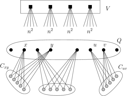
Figure 2: The graph $G^{\prime}$ in the transformation of the instances of Min Bisection to equivalent instances of Tree-cut Width.

Consider the set ${\cal C}=\{T_{1},\ldots,T_{\ell}\}$ of the connected components of $T\setminus\{q\}$ and let $e_{i}$ be the tree-edge between $T_{i}$ and $q$. As $w\geqslant|V(\bar{H}_{q})|\geqslant|Q|=w-2$, there are at most two tree-edges among $e_{1},\ldots,e_{\ell}$ such that $|\delta^{T}(e_{i})|\geqslant 3$. This means that there are at most two subtrees among $T_{1},\ldots,T_{\ell}$ such that $V\cap\bigcup_{t\in V(T_{i})}X_{t}\neq\emptyset$. From the fact that $|Q|=w-2$, at least $n-2$ vertices of $V$ are not contained in $X_{q}$ and thus there exists at least one subtree $T_{i}$ such that $V\cap\bigcup_{t\in V(T_{i})}X_{t}\neq\emptyset$. If there is $i$ such that $|V\cap\bigcup_{t\in V(T_{i})}X_{t}|\geqslant\frac{n}{2}+1$, then $|\delta^{T}(e_{i})|\geqslant(\frac{n}{2}+1)\cdot n^{2}>w$, a contradiction. Hence, we conclude that there are exactly two subtrees, say $T_{1}$ and $T_{2}$, in ${\cal C}$ such that $V\cap\bigcup_{t\in V(T_{i})}X_{t}\neq\emptyset$ for $i=1,2$ and for $3\leqslant i\leqslant\ell$, we have $V\cap\bigcup_{t\in V(T_{i})}X_{t}=\emptyset$. This, together with the fact that $|Q|=w-2$, enforces that the sets $V\cap\bigcup_{t\in V(T_{1})}X_{t}$ and $V\cap\bigcup_{t\in V(T_{2})}X_{t}$ make a bipartition of $V$ into sets of equal size. Let us call this bipartition $\{V_{1},V_{2}\}$. Observe that $\delta^{T}(e_{i})\supseteq\delta(V_{i},Q)\cup\delta(V_{1},V_{2})$, thus $\delta^{T}(e_{i})$ contains at least $\frac{n}{2}\cdot n^{2}+|\delta(V_{1},V_{2})|$ edges for $i=1,2$. As $|\delta^{T}(e_{1})|\leqslant w$, it follows $|\delta(V_{1},V_{2})|\leqslant k$. Therefore, $(G,k)$ is Yes-instance to Min Bisection  which complete the proof.

2.3 Tree-cut width vs treewidth

In this section we investigate the relation between treewidth and tree-cut width. The following was proved in [8].

Proposition 1

For a graph of tree-cut width at most $w$, its treewidth is at most $2w^{2}+3w$.

In the rest of this subsection we prove that the bound of Proposition 1 is asymptotically optimal. For this we need some definitions.

Let $G$ be a graph. Two subgraphs $X$ and $Y$ of $G$ touch each other if either $V(X)\cap V(Y)\neq\emptyset$ or there is an edge $e=\{x,y\}\in E(G)$ with $x\in V(X)$ and $y\in V(Y)$. A bramble ${\cal B}$ is a collection of connected subgraphs of $G$ pairwise touching each other. The order of a bramble ${\cal B}$ is the minimum size of a hitting set $S$ of ${\cal B}$, that is a set $S\subseteq V(G)$ such that for every $B\in{\cal B}$, $S\cap V(B)\neq\emptyset$. In Seymour and Thomas [17], it is known that the treewidth of a graph equals the maximum order over all brambles of $G$ minus one. Therefore, a bramble of order $k$ is a certificate that the treewidth is at least $k-1$.

We next define the family of graphs ${\cal H}=\{H_{w}:w\in{\mathbb{N}}_{\geqslant 1}\}$ as follows. The vertex set of $H_{w}$ is a disjoint union of $w$ cliques, $Q_{1},\ldots,Q_{w}$, each containing $w$ vertices. For each $1\leqslant i\leqslant w$, the vertices of $Q_{i}$ are labeled as $(i,j)$, $1\leqslant j\leqslant w$. Besides the edges lying inside the cliques $Q_{i}$’s, we add an edge between $(i,j)\in Q_{i}$ and $(j,i)\in Q_{j}$ for every $1\leqslant i<j\leqslant w$. Notice that the vertex $(i,i)$ does not have a neighbor outside $Q_{i}$. The graph $H_{4}$ is depicted in Fig. 3.

Figure 3: The graph $H_{4}$.

Lemma 1

The tree-cut width of $H_{w}$ is at most $w+1$.

Proof

Consider the tree-cut decomposition $(T,{\cal X})$, in which $T$ is a star with $t$ as the center and $q_{1},\ldots,q_{w}$ as leaves. For the bags, we set $X_{t}=\emptyset$, and $X_{q_{i}}=Q_{i}$ for $1\leqslant i\leqslant w$. It is straightforward to verify that the tree-cut width of $(T,{\cal X})$ is $w+1$.

Lemma 2

For any positive integer $w$, the treewidth of $H_{w}\in{\cal H}$ is at least $\frac{1}{16}w^{2}-1$.

Proof

For notational convenience, we assume that $w$ is even. The argument can be easily extended to the case when $w$ is odd. For $i\in[w]$ and a set $Z\subseteq[w]$, let $B(i,Z)$ denote the set $\{(i,j),(j,i):j\in Z\}$. We define ${\cal B}_{w}$ as

$${\cal B}_{w}=\{G[B(i,Z)]:\forall i\in[w],\ \forall Z\subseteq[w]\setminus\{i\}\text{\leavevmode\nobreak\ s.t.\leavevmode\nobreak\ }|Z|=w/2\}.$$

It is easy to verify that each subgraph of ${\cal B}_{w}$ is connected. For any $i\in[w]$ and $Z\subseteq[w]\setminus\{i\}$ such that $|Z|=\frac{1}{2}w$, the number of cliques $Q_{i}$, $1\leqslant i\leqslant w$, with which $B(i,Z)$ has non-empty intersection is at least $\frac{1}{2}w+1$. This means any two elements of ${\cal B}_{w}$ touch each other, and thus ${\cal B}_{w}$ is indeed a bramble. Henceforth, we show that the order of ${\cal B}_{w}$ is at least $\frac{1}{16}w^{2}$.

Suppose that there is a hitting set $S$ of ${\cal B}_{w}$ with $|S|<\frac{1}{16}w^{2}$. We define

$$F_{S}=\{i\in[w]\mid|\{j\in[w]:(j,i)\in V(G)\setminus S\}|\geqslant\frac{3}{4}w\}.$$

Claim 1

$|F_{S}|>\frac{3}{4}w$.

Proof of the Claim: Suppose that the contrary holds. We use a counting argument to derive a contradiction. The set $V(G)\setminus S$ is partitioned into two sets: $\{(j,i):j\in[w],i\in F_{S}\}$ and $\{(j,i):j\in[w],i\not\in F_{S}\}$. We have

$$|V(G)\setminus S|\leqslant w\cdot|F_{S}|+\frac{3}{4}w\cdot(w-|F_{S}|)\leqslant\frac{3}{4}w^{2}+\frac{3}{16}w^{2}=\frac{15}{16}w^{2},$$

contradicting to the assumption that $|S|<\frac{1}{16}w^{2}$. $\Diamond$

Claim 2

There exists $i^{*}\in F_{S}$ such that $|\{j\in[w]:(i^{*},j)\in S\}|<\frac{1}{4}w$.

Proof of the Claim: Suppose the contrary, i.e. we have $|\{j\in[w]:(i,j)\in V(G)\setminus S\}|\leqslant\frac{3}{4}w$ for every $i\in F_{S}$. Notice that the set $V(G)\setminus S$ is partitioned into $\{(i,j):i\in F_{S},j\in[w]\}$ and $\{(i,j):i\in[w]\setminus F_{S},j\in[w]\}$. Then,

$$|V(G)\setminus S|\leqslant|F_{S}|\cdot\frac{3}{4}w+(w-|F_{S}|)\cdot w\leqslant w^{2}-\frac{1}{4}w\cdot|F_{S}|<\frac{13}{16}w^{2},$$

where the last inequality follows from Claim 1. This contradicts the assumption that $|S|<\frac{1}{16}w^{2}$. $\Diamond$

Consider some $i^{*}\in F_{S}$ satisfying the condition of Claim 2. We observe that the set

$$Z=\{j\in[w]:(j,i^{*})\in V(G)\setminus S\}\setminus(\{i^{*}\}\cup\{j\in[w]:(i^{*},j)\in S\})$$

contains at least $\frac{1}{2}w$ vertices by the definition of $F_{S}$ and Claim 2. Pick any subset $Z^{*}$ of $Z$ of size exactly $\frac{1}{2}w$. To reach a contradiction, it suffices to show that $B(i^{*},Z^{*})\cap S=\emptyset$. Indeed, from the fact that $Z^{*}\subseteq\{j\in[w]:(j,i^{*})\in V(G)\setminus S\}$, it follows that

$$\forall j\in Z^{*}\ (j,i^{*})\in V(G)\setminus S.$$ (1)

By the definition of $Z$ it follows that $Z^{*}\cap\{j\in[w]:(i^{*},j)\in S\}=\emptyset,$ which, implies that

$$\forall j\in Z^{*}\ (i^{*},j)\in V(G)\setminus S.$$ (2)

By (1) and (2), we conclude that $B(i^{*},Z^{*})\cap S=\emptyset$. This completes the proof.

From Lemmata 1 and 2, we conclude to the following.

Theorem 2.2

For every $w\in{\mathbb{N}}_{\geqslant 1}$ there exists a graph $H_{w}$ such that $\mathbf{tw}(H_{w})={\rm\Omega}((\mbox{\bf tcw}(H_{w}))^{2})$.

3 The 2-approximation algorithm

We present a 2-approximation of Tree-cut Width running in time $2^{O(w^{2}\log w)}\cdot n^{2}$. As stated in Lemma 3 below, we first observe that computing the tree-cut width of $G$ reduces to computing the tree-cut width of 3-edge-connected graphs. This property can be easily derived from [23, Lemmas 10–11].

Lemma 3

Given a connected graph $G$, let $\{V_{1},V_{2}\}$ be a partition of $V(G)$ such that $\delta_{G}(V_{1},V_{2})$ is a minimal cut of size at most two and let $w\geqslant 2$ be a positive integer. For $i=1,2$, let $G_{i}$ be the graph obtained from $G$ by identifying the vertex set $V_{3-i}$ into a single vertex $v_{3-i}$. Then $G$ has tree-cut width at most $w$ if and only if both $G_{1}$ and $G_{2}$ have tree-cut width at most $w$.

Proof

Recall that $\textbf{tcw}(H)\leqslant\textbf{tcw}(G)$ if $G$ admits an immersion of $H$ by [23, Lemma 11]. Hence, in order to prove the forward implication, it suffices to prove that $G_{i}$ is an immersion of $G$, for $i=1,2$. If $|\delta(V_{1},V_{2})|=1$, for each $i=1,2$ we can delete all vertices of $V_{3-i}$ except for the single vertex in $N(V_{i})$ and obtained $G_{i}$. If $|\delta(V_{1},V_{2})|=2$, note that for each $i=1,2$, $G[V_{3-i}]$ is connected and thus $G_{i}$ can be obtained by deleting vertices, edges and lifting a sequence of edges along the path between two vertices in $N(V_{i})$.

Conversely, let $(T^{i},{\cal X}^{i})$ be a tree-cut decomposition of $G_{i}$ of width at most $w$ for $i=1,2$, and consider the tree-cut decomposition $(T,{\cal X})$ such that ${\cal X}={\cal X}_{1}\cup{\cal X}_{2}$ and $T$ is obtained by the disjoint union of $T^{1}$ and $T^{2}$ after adding an edge between $t_{1}\in V(T^{1})$ and $t_{2}\in V(T^{2})$, where $t_{i}$ is the tree node of $T_{i}$ containing $v_{3-i}$, i.e. the vertex obtained by contracting $V_{3-i}$. We remove $v_{1}$ and $v_{2}$ from the bags of $T$.

We claim that $(T,{\cal X})$ is a tree-cut decomposition of width at most $w$. Note first that the adhesion of $(T,{\cal X})$ is at most $w$ since $|\delta^{T}(\{t_{1},t_{2}\})|\leqslant 2$ and the adhesion of $(T^{i},{\cal X}^{i})$ is at most $w$ for $i=1,2$. From $|\delta^{T}(\{t_{1},t_{2}\})|\leqslant 2$, it follows that for $i=1,2$, the 3-center of $(H_{t_{i}},X_{t_{i}})$ of the tree-decomposition $(T,{\cal X})$ is the same as the 3-center of $(H_{t_{i}},X_{t_{i}})$ of the tree-decomposition $(T^{i},{\cal X}^{i})$. Therefore the width of $(T,{\cal X})$ is at most $w$.

The proof of the next lemma is easy and is omitted.

Lemma 4

Let $G$ be a graph and let $v$ be a vertex of $G$ with degree 1 (resp. 2). Let also $G^{\prime}$ be the graph obtained from $G$ after removing (resp. dissolving) $v$. Then $\mbox{\bf tcw}(G)=\mbox{\bf tcw}(G^{\prime})$.

From now on, based on Lemmata 3 and 4, we assume that the input graph is $3$-edge-connected. In this special case, the following observation is not difficult to verify. It allows us to work with a slightly simplified definition of the $3$-centers in a tree-cut decomposition.

Observation 1

Let $G$ be a 3-edge-connected graph and let $(T,\cal{X})$ be a tree-cut decomposition of $G$. Consider an arbitrary node $t$ of $V(T)$ and let ${\cal T}$ be the set containing every connected component $T^{\prime}$ of $T\setminus t$ such that $\bigcup_{s\in V(T^{\prime})}X_{s}\neq\emptyset.$ Then $|V(\bar{H}_{t})|=|X_{t}|+|{\cal T}|,$ that is $|V(\bar{H}_{t})|=|V({H}_{t})|$.

We observe that the proof of Lemma 3 provides a way to construct a desired tree-cut decomposition for $G$ from decompositions of smaller graphs. Given an input graph $G$ for Tree-cut Width, we find a minimal cut $(V_{1},V_{2})$ with $|\delta(V_{1},V_{2})|\leqslant 2$ and create a graph $G_{i}$ as in Lemma 3, with the vertex $v_{3-i}$ marked as distinguished. We recursively find such a minimal cut in the smaller graphs created until either one becomes 3-edge-connected or has at most $w$ vertices.

Therefore, a key feature of an algorithm for Tree-cut Width lies in how to handle 3-edge-connected graphs. Our algorithm iteratively refines a tree-cut decomposition $(T,\mathcal{X})$ of the input graph $G$ and either guarantees that the following invariant is satisfied or returns that $\mbox{\bf tcw}(G)>\omega$.

Invariant: $(T,\mathcal{X})$ is a tree-cut decomposition of $G$ where $\mathbf{in}\text{-}\mathbf{tcw}(T,\mathcal{X})\leqslant 2\cdot w$.

Clearly the trivial tree-cut decomposition satisfies the Invariant. A leaf $t$ of $T$ such that $|X_{t}|\geqslant 2\cdot\omega$ is called a large leaf. At each step, the algorithm picks a large leaf and refines the current tree-cut decomposition by breaking this leaf bag into smaller pieces. The process repeats until we finally obtain a tree-cut decomposition of width at most $2w$, or encounter a certificate that $\textbf{tcw}(G)>w$.

3.1 Refining a large leaf of a tree-cut decomposition

A large leaf will be further decomposed into a star. To that aim, we will solve the following problem:

Constrained Star-Cut Decomposition
Input: An undirected graph $G$, an integer $w\in\mathbb{N}$, a set $B\subseteq V(G)$, and a weight function $\gamma:B\rightarrow\mathbb{N}$.

Parameter: $w$.
Output: A non-trivial tree-cut decomposition $(T,\mathcal{X})$ of $G$ such that

1. $T$ is a star with central node $t_{c}$ and with $\ell$ leaves for some $\ell\in\mathbb{N}^{+}$,

2. $\mathbf{in}\text{-}\mathbf{tcw}(T,\mathcal{X})\leqslant w$, and

3. $|X_{t_{c}}|+\ell\leqslant w$ and for every leaf node $t$, $\gamma(B\cap X_{t})\leqslant w$,

or report that such a tree-cut decomposition does not exist.

Observe that a Yes-instance satisfies, for every $x\in B$, $\gamma(x)\leqslant w$. We also notice that as the output of the algorithm is a non-trivial tree-cut decomposition, $T$ contains at least two nodes with non-empty bags and every leaf node is non-empty.

Given a subset $S\subseteq V(G)$, we define the instance of the Constrained Star-Cut Decomposition problem $I(S,G)=(G[S],w,\partial_{G}(S),\gamma_{S})$ where for every $x\in\partial_{G}(S)$, $\gamma_{S}(x)=|\delta_{G}(\{x\},V(G)\setminus S)|$.

Lemma 5

Let $G$ be a 3-edge-connected graph, $w\in\mathbb{Z}_{\geqslant 2}$, and let $S\subseteq V(G)$ be a set of vertices such that $|S|\geqslant w+1$ and $|\delta_{G}(S,V(G)\setminus S)|\leqslant 2w$. If ${\bf tcw}(G)\leqslant w$, then $I(S,G)=(G[S],w,\partial_{G}(S),\gamma_{S})$ is a Yes-instance of Constrained Star-Cut Decomposition.

Proof

Let $(T,{\cal X})$ be a normalized tree-cut decomposition of $G$ of width at most $w$. We extend the weight function $\gamma_{S}$ on $\partial_{G}(S)$ into $\gamma^{\prime}_{S}$ on $V(G)$ by setting $\gamma^{\prime}_{S}(v)=\gamma_{S}(v)$ for every $v\in S$ and $\gamma^{\prime}_{S}(v)=0$ otherwise. Also, given a subtree $T^{\prime}$ of $T$, we let $\gamma_{S}^{\prime}(T^{\prime})=\sum_{t\in V(T^{\prime})}\sum_{v\in X_{t}}\gamma_{S}^{\prime}(v)$. The idea is to identify a node $t_{c}$ of $T$ that will serve as the central node of the star decomposition. The leaves of the star decomposition will results from the contraction of the subtrees of $T\setminus t_{c}$ containing bags that intersect the set $S$. To find the node $t_{c}$, we orient the edges of $T$ using the following two rules. Given an edge $e=\{x,y\}\in E(T)$:

1. Rule 1: orient $e$ from $x$ to $y$ if $\gamma_{S}^{\prime}(T_{y})>w$.

2. Rule 2: orient $e$ from $x$ to $y$ if $S\cap\bigcup_{t\in V(T_{x})}X_{t}=\emptyset$.

Let $\vec{T}$ be the resulting orientation of $T$. Observe that Rule 1 and 2 may leave some edges of $T$ non-oriented.

Claim 3

For every edge $e=\{x,y\}$ of $T$, $e$ is oriented either in a single direction or not oriented in $\vec{T}$.

Proof of the Claim: Observe that if Rule 1 orients $e$ from $x$ to $y$, neither Rule 1 nor Rule 2 may orient $e$ in the opposite direction. The former is an immediate consequence of the fact $\gamma_{S}^{\prime}(T_{x})+\gamma_{S}^{\prime}(T_{y})=|\delta_{G}(S,V(G)\setminus S)|\leqslant 2w$. Rule 2 does not orient $e$ from $y$ to $x$ either: if Rule 2 does so, we have $S\cap\bigcup_{t\in V(T_{y})}X_{t}=\emptyset$ and since the value $\gamma_{S}^{\prime}(v)$ is non-zero only when $v\in S$, we conclude that $\gamma_{S}(T_{y})=0$, a contradiction to the assumption that Rule 1 oriented $e$ from $x$ to $y$. Moreover, the edge $e$ cannot be oriented in both directions by Rule 2 since $S$ is non-empty and thus at least one of the sets $\bigcup_{t\in V(T_{x})}X_{t}$ and $\bigcup_{t\in V(T_{y})}X_{t}$ intersects with $S$. $\Diamond$

By Claim 3, $\vec{T}$ contains at least one node, say $t_{c}$, which is not incident to an out-going edge in $\vec{T}$. Let $T_{1},\ldots,T_{\ell}$ be the connected components of $T\setminus t_{c}$ containing a node $t$ such that $X_{t}\cap S\neq S$. Observe that as $|S|\geqslant w+1$ and $\mbox{\bf tcw}(T,\mathcal{X})=w$, $S$ cannot be included in a single bag of $(T,\mathcal{X})$ and thereby $\ell\geqslant 1$. Consider the following tree-cut decomposition $(T^{*},\mathcal{X}^{*})$ of $G[S]$:

• $T^{*}$ is a star with central node $t_{c}$ and leaf nodes $t_{1}\dots t_{\ell}$,

• the bag of node $t_{c}$ is $X^{*}_{c}=X_{t_{c}}\cap S$,

• for every leaf node $t_{i}\in V(T^{*})$, we set $X^{*}_{i}=\bigcup_{t\in V(T_{i})}X_{t}\cap S$.

Observe that $(T^{*},\mathcal{X}^{*})$ is a tree-cut decomposition of $G[S]$ and since $|S|\geqslant w+1$, it is non-trivial. By construction, as it is obtained from $(T,\mathcal{X})$ by contracting subtrees and removing vertices from bags, we have that $\mathbf{in}\text{-}\mathbf{tcw}(T^{*},\mathcal{X}^{*})\leqslant w$. It remains to prove that $|X_{t_{c}}|+\ell\leqslant w$ and that $\gamma_{S}(\partial_{G}(S)\cap X_{t})\leqslant w$ for every leaf node $t$. The former inequality directly follows from Observation 1 and the fact that $(T,\mathcal{X})$ is an optimal tree-cut decomposition of $G$. The latter inequality follows from the fact that $t$ does not have an out-going edge in $\vec{T}$, in particular, Rule 1 does not orient any edge incident with $t$ outwardly from $t$.

Given a $3$-edge-connected graph, applying Lemma 5 on a large leaf of a tree-cut decomposition that satisfies the Invariant, we obtain:

Corollary 1

Let $G$ be a 3-edge-connected graph $G$ such that $\mathbf{tcw}(G)\leqslant w$, and let $t$ be a large leaf of a tree-cut decomposition $(T,\mathcal{X})$ satisfying the Invariant. Then $I(X_{t},G)=(G[X_{t}],w,\partial_{G}(X_{t}),\gamma_{X_{t}})$ is a Yes-instance of Constrained Star-Cut Decomposition.

The next lemma shows that if a large leaf bag $X_{t}$ of a tree-cut decomposition $(T,\mathcal{X})$ satisfying the Invariant defines a Yes-instance of the Constraint Tree-Cut Decomposition problem, then $(T,\mathcal{X})$ can be further refined.

Lemma 6

Let $G$ be a 3-edge-connected graph $G$ and $(T,\mathcal{X})$ be tree-cut decomposition of satisfying the Invariant. If $(T^{*},\mathcal{X}^{*})$ is a solution of Constrained Star-Cut Decomposition on the instance $I(X_{t},G)=(G[X_{t}],w,\partial_{G}(X_{t}),\gamma_{X_{t}})$ where $t$ is a large leaf of $(T,\mathcal{X})$, then the pair $(\tilde{T},\tilde{\mathcal{X}})$ where

• $V(\tilde{T})=(V(T)\setminus\{t\})\cup V(T^{*})$,

• $E(\tilde{T})=(E(T)\setminus\{(t,t^{\prime})\})\cup E(T^{*})\cup\{(t_{c},t^{\prime})\}$, where $t^{\prime}$ is the unique neighbor of $t$ in $T$ and $t_{c}$ is the central node of $T^{*}$,

• $\tilde{\cal X}=({\cal X}\setminus\{X_{t}\})\cup{\cal X}^{*}$

is a tree-cut decomposition of $G$ satisfying the Invariant. Moreover the number of non-empty bags is strictly larger in $(\tilde{T},\tilde{\mathcal{X}})$ than in $(T,\mathcal{X})$.

Proof

By construction, $(\tilde{T},\tilde{\mathcal{X}})$ is a tree-cut decomposition of $G$. The fact that $(T^{*},\mathcal{X}^{*})$ is non-trivial implies that the number of non-empty bags is strictly larger in $(\tilde{T},\tilde{\mathcal{X}})$ than in $(T,\mathcal{X})$.

It remains to prove that $\mathbf{in}\text{-}\mathbf{tcw}(\tilde{T},\tilde{\mathcal{X}})\leqslant 2\cdot w$. Since $(T^{*},\mathcal{X}^{*})$ is a solution to $I(X_{t},G)$, we have $|X^{*}_{t_{c}}|+\ell\leqslant w$. As $G$ is edge $3$-connected, by Observation 1, the torso size at $t_{c}$ in $(\tilde{T},\tilde{\mathcal{X}})$ at most $w+1$, which is at most $2w$. Let us verify that the adhesion of $(\tilde{T},\tilde{\mathcal{X}})$ is at most $2w$. For this, it suffices to bound the value $|\delta^{\tilde{T}}(e)|$ for the newly created edges $e=\{t_{i},t_{c}\}$, for all $i\in[\ell]$. We have

$$|\delta^{\tilde{T}}(\{t_{i},t_{c}\})| =|\delta_{G}(\tilde{X}_{t_{i}},V(G)\setminus\tilde{X}_{t_{i}})|$$

$$=|\delta_{G}(\tilde{X}_{t_{i}},X_{t}\setminus\tilde{X}_{t_{i}})|+|\delta_{G}(\tilde{X}_{t_{i}},V(G)\setminus X_{t})|\leqslant 2w.$$

The inequality follows from that $(T^{*},\mathcal{X}^{*})$ is a solution to $I(X_{t},G)$. More precisely, $|\delta_{G}(\tilde{X}_{t_{i}},X_{t}\setminus\tilde{X}_{t_{i}})|\leqslant w$ is implied by the fact that $\mathbf{in}\text{-}\mathbf{tcw}(T^{*};\mathcal{X})\leqslant w$. And $|\delta_{G}(\tilde{X}_{t_{i}},V(G)\setminus X_{t})|\leqslant w$ is a consequence of $\gamma_{X_{t}}(\partial_{G}(X_{t})\cap X^{*}_{t_{i}})\leqslant w$.

Finally, as $(T^{*},\mathcal{X}^{*})$ is a non-trivial tree-cut decomposition, the number of non-trivial nodes is strictly larger in $(\tilde{T},\tilde{\mathcal{X}})$ than in $(T,\mathcal{X})$.

3.2 An FPT algorithm for Constrained Star-Cut Decomposition

Lemma 1 provides a quadratic bound on the treewidth of a graph in term of its tree-cut width. This allows us to develop a dynamic programming algorithm for solving Constrained Star-Cut Decomposition on graphs of bounded treewidth. To obtain a tree-decomposition, we use the 5-approximation FPT-algorithm of the following proposition.

Proposition 2 (see [2])

There exists an algorithm which, given a graph $G$ and an integer $k$, either correctly decides that ${\bf tw}(G)>w$ or outputs a tree-decomposition of width at most $5w+4$ in time $2^{O(w)}\cdot n$.

If $\mbox{\bf tcw}(G)\leqslant w$, then by Lemma 1 $\mathbf{tw}(G)\leqslant 2w^{2}+3w$. From Proposition 2, we may assume that $G$ has treewidth $O(w^{2})$ and, based on this and the next lemma, solve Constrained Star-Cut Decomposition in $2^{O(w^{2}\cdot\log w)}\cdot n$ steps.

A rooted tree decomposition $(T,{\cal X},r)$ is a tree decomposition with a distinguished node $r$ selected as the root. A nice tree decomposition $(T,{\cal Y},r)$ (see [13]) is a rooted tree decomposition where $T$ is binary, the bag at the root is $\emptyset$, and for each node $x$ with two children $y,z$ it holds $Y_{x}=Y_{y}=Y_{z}$, and for each node $x$ with one child $y$ it holds $Y_{x}=Y_{y}\cup\{u\}$ or $Y_{x}=Y_{y}\setminus\{u\}$ for some $u\in V(G)$. Notice that a nice tree decomposition is always a rooted tree decomposition. We need the following proposition.

Proposition 3 (see [1])

For any constant $k\geqslant 1$, given a tree decomposition of a graph $G$ of width $\leqslant k$ and $O(|V(G)|)$ nodes, there exists an algorithm that, in $O(|V(G)|)$ time, constructs a nice tree decomposition of $G$ of width $\leqslant k$ and with at most $4|V(G)|$ nodes.

Lemma 7

Let $(G,w,B,\gamma)$ be an input of Constrained Star-Cut Decomposition and let $\mathbf{tw}(G)\leqslant q$. There exists an algorithm that given $(G,w,B,\gamma)$ outputs, if one exists, a solution of $(G,w,B,\gamma)$ in $2^{O((q+w)\log w)}\cdot n$ steps.

Sketch of proof: From Proposition 3, we can assume that we are given a nice tree-decomposition $(T,{\cal Y},r)$ of $G$ of width at most $O(q)$, which can be obtained in time $2^{O(q)}\cdot n$ because of Proposition 2. We describe dynamic programming tables. Let $Z_{t}$ be the vertex set $\bigcup_{t^{\prime}\in V(T_{t})}Y_{t^{\prime}}$, where $T_{t}$ is the subtree of $T$ rooted at $t$. For every $1\leq\ell\leq w$, we need to compute a collection $\mathcal{X}=\{X_{0},\dots,X_{\ell}\}$ of pairwise disjoint subsets of $V(G)$ (some of them may be empty sets) such that $|X_{0}|+\ell\leqslant w$. The subset $X_{0}$ will play the role of the bag of the central node of the star-cut decomposition.

To guarantee that the specification of the problem can be checked, the dynamic programming table at node $t$ will store a collection of quadruples $(\phi,a,\alpha,\beta)$ with the following specifications:

• $\phi:Y_{t}\rightarrow[0,\ell]$, indicating that $x\in Y_{t}$ belongs to $X_{\phi(x)}\cap Z_{t}$;

• $a$ is a number indicating the size $|X_{0}\cap Z_{t}|$ of the central bag in $G[Z_{t}]$;

• $\alpha:[\ell]\rightarrow[0,w]$ is a function, indicating the weight $\gamma(B\cap X_{i}\cap Z_{t})$;

• $\beta:[\ell]\rightarrow[0,w]$ is a function, indicating $|\delta(X_{i},Z_{t}\setminus X_{i})|$;

Suppose that we have constructed tables for all nodes of $T$ such that: for every node $t$, a quadruple $(\phi,a,\alpha,\beta)$ appears in the table at node $t$ if and only if there exists a collection $\mathcal{X}^{\prime}=\{X^{\prime}_{0},\dots X^{\prime}_{\ell}\}$ meeting the specifications. It is not difficult to see that the instance $(G,w,B,\gamma)$ is Yes if and only if the table at the root contains a quadruple $(\phi,a,\alpha,\beta)$ such that $\ell+a\leq w$. Furthermore, such tables can be constructed using standard dynamic programming in a bottom-up manner.

Observe that the size of the dynamic table at each node $t$ is dominated by the number of collections $\mathcal{X}=\{X_{0},\dots X_{\ell}\}$ of pairwise disjoint subsets of $Y_{t}$, with $\ell\leqslant w$, which is $2^{O((q+w)\log w)}$. Maintaining these tables follows by a standard dynamic programming algorithm. $\square$

3.3 Piecing everything together

We now present a 2-approximation algorithm for Tree-cut Width leading to the following result.

Theorem 3.1

There exists an algorithm that, given a graph $G$ and a $w\in\mathbb{Z}_{\geqslant 0}$, either outputs a tree-cut decomposition of $G$ with width at most $2w$ or correctly reports that no tree-cut decomposition of $G$ with width at most $w$ exists in $2^{O(w^{2}\cdot\log w)}\cdot n^{2}$ steps.

Proof

Recall that, by Lemmata 3 and 4, we can assume that $G$ is $3$-edge-connected. If not, we iteratively decompose $G$ into 3-edge-connected components using the linear-time algorithm of [22]. A tree-cut decomposition of $G$ can easily built from the tree-cut decomposition of its $3$-edge-connected components using Lemma 3. As mentioned earlier, the trivial tree-cut decomposition satisfies the Invariant. Let $(T,\mathcal{X})$ be a tree-cut decomposition satisfying the Invariant. As long as the current tree-cut decomposition $(T,\mathcal{X})$ contains a large leaf $\ell$, the algorithm applies the following steps repeatedly:

1. Let $X_{\ell}\in\mathcal{X}$ be the bag associated to a large leaf $\ell$. Compute a nice tree-decomposition of $G[X_{\ell}]$ of width at most $O(w^{2})$ in $2^{O(w^{2})}\cdot n$ time. If such a decomposition does not exist, as $G[X_{\ell}]$ is a subgraph of $G$, Lemma 1 implies $\mbox{\bf tcw}(G)>w$ and the algorithm stops.

2. Solve Constrained Star-Cut Decomposition on $I(X_{t},G)$ using the dynamic programming of Lemma 7 for $q=O(w^{2})$ in time $2^{O(w^{2}\cdot\log w)}\cdot n$.

3. If $I(X_{t},G)$ is a NO-instance, then by Corollary 1, $\mbox{\bf tcw}(G)>w$ and the algorithm stops.

4. Otherwise, by Lemma 6, $(T,\mathcal{X})$ can be refined into a new tree-cut decomposition satisfying the Invariant.

The algorithm either stops when we can correctly report that $\mbox{\bf tcw}(G)>w$ (step 1 or 3) or when the current tree-cut decomposition has no large leaf. In the latter case, as $(T,\cal{X})$ satisfies (*), it holds that $\mbox{\bf tcw}(T,\mathcal{X})\leqslant 2\cdot w$. Observe that each refinement step (step 4) strictly increases the number of non-empty bags (see Lemma 6). It follows that the above steps are repeated at most $n$ times, implying that the running time of the 2-approximation algorithm is $2^{O(w^{2}\cdot\log w)}\cdot n^{2}$.

4 Open problems

The main open question is on the possibility of improving the running time or the approximation factor of our algorithm. Notice that the parameter dependence $2^{O(w^{2}\cdot\log w)}$ is based on the fact that the tree-cut width is bounded by a quadratic function of treewidth. As we proved (Theorem 2.2), there is no hope of improving this upper bound. Therefore any improvement of the parametric dependence should avoid dynamic programming on tree-decompositions or significantly improve the running time. Another issue is whether we can improve the quadratic dependence on $n$ to a linear one. In this direction we actually believe that an exact FPT-algorithm for the tree-cut width can be constructed using the “set of characteristic sequences” technique, as this was done for other width parameters [20, 21, 3, 4, 19, 12]. However, as this technique is more involved, we believe that it would imply a higher parametric dependence than the one of our algorithm.

Acknowledgement. We would like to thank the reviewers of the extended abstract of this work for helpful remarks that improved the presentation of the manuscript.

References

- [1] H. L. Bodlaender. A linear time algorithm for finding tree-decompositions of small treewidth. SIAM Journal on Computing, 25:1305–1317, 1996.
- [2] H. L. Bodlaender, P. G. Drange, M. S. Dregi, F. Fomin, D. Lokshtanov, and M. Pilipczuk. An -approximation algorithm for treewidth. In IEEE Symposium on Foundations of Computer Science, FOCS, pages 499–508, 2013.
- [3] H. L. Bodlaender and T. Kloks. Efficient and constructive algorithms for the pathwidth and treewidth of graphs. Journal of Algorithms, 21(2):358–402, 1996.
- [4] H. L. Bodlaender and D. M. Thilikos. Computing small search numbers in linear time. In International Workshop on Parameterized and Exact Computation, IWPEC, volume 3162 of Lecture Notes in Computer Science, pages 37–48. 2004.
- [5] B. Courcelle. The monadic second-order logic of graphs. I. Recognizable sets of finite graphs. Information and Computation, 85(1):12–75, 1990.
- [6] M. Dom, D. Lokshtanov, S. Saurabh, and Y. Villanger. Capacitated domination and covering: A parameterized perspective. In International Workshop on Parameterized and Exact Computation, IWPEC, volume 5018 of Lecture Notes in Computer Science, pages 78–90. 2008.
- [7] M. R. Fellows, F. V. Fomin, D. Lokshtanov, F. Rosamond, S. Saurabh, S. Szeider, and C. Thomassen. On the complexity of some colorful problems parameterized by treewidth. Information and Computation, 209(2):143–153, 2011.
- [8] R. Ganian, E. J. Kim, and S. Szeider. Algorithmic applications of tree-cut width. In International Symposium on Mathematical Foundations of Computer Science, MFCS, to appear in Lecture Notes in Computer Science, 2015.
- [9] M. R. Garey and D. S. Johnson. Computers and intractability. A guide to the theory of NP-completeness. 1979.
- [10] P. A. Golovach and D. M. Thilikos. Paths of bounded length and their cuts: Parameterized complexity and algorithms. Discrete Optimization, 8(1):72–86, 2011.
- [11] M. Grohe, K. Kawarabayashi, D. Marx, and P. Wollan. Finding topological subgraphs is fixed-parameter tractable. In ACM Symposium on Theory of Computing, STOC, pages 479–488, 2011.
- [12] J. Jeong, E. J. Kim, and S. Oum. Constructive algorithm for path-width of matroids. CoRR abs/1507.02184, 2015.
- [13] T. Kloks. Treewidth. Computations and Approximations, volume 842 of LNCS. Springer, 1994.
- [14] N. Robertson and P. D. Seymour. Graph minors. III. Planar tree-width. Journal of Combinatorial Theory, Series B, 36(1):49–64, 1984.
- [15] N. Robertson and P. D. Seymour. Graph minors. V. Excluding a planar graph. Journal of Combinatorial Theory, Series B, 41(1):92–114, 1986.
- [16] N. Robertson and P. D. Seymour. Graph minors. XXIII. Nash-Williams’ immersion conjecture. Journal of Combinatorial Theory, Series B, 100(2):181–205, 2010.
- [17] P. D. Seymour and R. Thomas. Graph searching and a min-max theorem for tree-width. Journal of Combinatorial Theory, Series B, 58(1):22–33, 1993.
- [18] P. D. Seymour and R. Thomas. Call routing and the ratcatcher. Combinatorica, 14(2):217–241, 1994.
- [19] R. P. Soares. Pursuit-evasion, decompositions and convexity on graphs. PhD thesis, COATI, INRIA/I3S-CNRS/UNS Sophia Antipolis, France and ParGO Research Group, UFC Fortaleza, Brazil, 2014.
- [20] D. M. Thilikos, M. J. Serna, and H. L. Bodlaender. Cutwidth I: A linear time fixed parameter algorithm. Journal of Algorithms, 56(1):1–24, 2005.
- [21] D. M. Thilikos, M. J. Serna, and H. L. Bodlaender. Cutwidth II: Algorithms for partial -trees of bounded degree. Journal of Algorithms, 56(1):25–49, 2005.
- [22] T. Watanabe, S. Taoka, and T. Mashima. Minimum-cost augmentation to 3-edge-connect all specified vertices in a graph. In ISCAS, pages 2311–2314, 1993.
- [23] P. Wollan. The structure of graphs not admitting a fixed immersion. Journal of Combinatorial Theory, Series B, 110:47–66, 2015.