Effects of $NN$ potentials on $p$ nuclides in the A$\sim$100-120 region

Abstract

Microscopic optical potentials for low energy proton reactions have been obtained by folding density dependent M3Y interaction derived from nuclear matter calculation with densities from mean field approach to study astrophysically important proton rich nuclei in mass 100-120 region. We compare S factors for low-energy $(p,\gamma)$ reactions with available experimental data and further calculate astrophysical reaction rates for $(p,\gamma)$ and $(p,n)$ reactions. Again we choose some nonlinear R3Y interactions from RMF calculation and folded them with corresponding RMF densities to reproduce experimental S factor values in this mass region. Finally the effect of nonlinearity on our result is discussed.

I Introduction

In nature 35 nuclei, commonly termed as $p$ nuclei, can be found on the proton-rich side of the nuclear landscape ranging between ⁷⁴Se to ¹⁹⁶Hg. As they are neutron deficit, the astrophysical reactions involved in the synthesis of these elements do not correspond to the slow($s$) or fast($r$) neutron capture processes. It mainly includes reactions such as proton capture, charge exchange and photo-disintegration. One can find a detailed study related to the $p$ process in standard textbooks [for example, Illiadisili ] and reviewsprev .

The natural abundances for $p$ nuclei are very low in the order of 0.01% to 1%. In general, the calculation of isotopic abundances require a network calculation typically involving 2000 nuclei and approximately 20000 reaction and decay channels and one major problem with this $p$ network is that most of the nuclei involved in the reaction network are very shortly lived. As a consequence, it is very difficult to track the $p$ process nucleosynthesis network experimentally. However, recent radioactive ion beam facilities are giving new prospects, still we are far away from measuring astrophysical reaction rates for the main reactions involved in the $p$ process. Thus, one often has to depend on theoretical models to study these reactions. These type of calculations acutely exploit the Hauser-Feshbach formalism where the optical model potential, in a local or a global form, is a key ingredient. Rauscher et al. substantially calculated astrophysical reaction rates and cross sections in a global approachrate . They further made a comment that the statistical model calculations may be improved by using locally tuned parameterization.

In this manuscript, we perform a fully microscopic calculation. The framework is based on microscopic optical model utilizing the theoretical density profile of a nucleus. In presence of a stable target, electron scattering experiment can be performed to avail nuclear charge density distribution data. However, in absence of a stable target, theory remains a sole guide to describe the density. Therefore, in this work we employ relativistic mean field (RMF) approach to extract the density information of a nucleus. This has the advantage of extending it to unknown mass regions. In some earlier worksgg ; clah1 ; clah2 ; clah3 ; saumi , this method has been used to study low energy proton reactions in the A $\sim$ 55-100 region. In a recent workdipti , similar method has been used in 110-125 mass region.

The nonlinearity in the scalar fieldrein ; sahu in a RMF theory has been proved very successful in reproducing various observables like nuclear ground state including nuclear matter properties and the surface phenomena like proton radioactivity etc. In the present work, we intend to study the effect of microscopic optical potentials obtained from nonlinear $NN$ interactions also in addition to the conventional linear $NN$ interactions in the A$\sim$ 100-120 region. In this work, we concentrate mainly on the region relevant to the $p$ network and therefore mainly proton rich and stability region of the nuclear landscape is our main concern.

II Technique

The RMF approach has successfully explained various features of stable and exotic nuclei like ground state binding energy, radius, deformation, spin-orbit splitting, neutron halo etc walecka74 ; pring96 ; bender03 ; soret86 ; miller72 . The RMF theory is nothing but the relativistic generalization of the non-relativistic effective theory like Skyrme and Gogny approach. This theory does the same job, what the non-relativistic theory can do, with an additional guarantee that it works in a better way in high density regioncompare . In this manuscript we have used the RMF formalism in both direct and indirect way. Directly we have calculated the nuclear density, which is an essential quantity to calculate the optical potential. Indirectly we used RMF Lagrangian to derive $NN$ interactions also along with the phenomenologically availed $NN$ interaction model. Here we have used different types of $NN$ interactions, namely the density dependent M3Y interaction (DDM3Y) and nonlinear R3Y interactions(NR3Y). The concept of the NR3Y was originally developed from basic idea of the RMF formalismbhuyan12 and will be discussed later in this section.

In order to calculate the nuclear density, different forms of Lagrangian densities can be used from RMF approach. In this manuscript, the chosen form of the interaction Lagrangian density is given by

$${\cal L}_{int} = \bar{{\psi}}\bigg{[}{g_{\sigma}}{\phi}-\bigg{(}{g_{\omega}}{V_{\mu}}+\frac{g_{\rho}}{2}{\tau}.{\mathbf{b}_{\mu}}+\frac{e}{2}(1+\tau_{3}){A_{\mu}}\bigg{)}\gamma_{\mu}\bigg{]}{\psi}$$ (1)

$$- \frac{g_{2}}{3}{\phi^{3}}-\frac{g_{3}}{4}\phi^{4}+\frac{\xi}{4}({V_{\mu}}{V^{\mu}})^{2}$$

$$+ \Lambda(\mathbf{b}_{\mu}.\mathbf{b}^{\mu})(V_{\mu}V^{\mu}).$$

Here $m_{\sigma}$, $m_{\rho}$, $m_{\omega}$ are the masses of the various mesons like sigma, rho, and omega respectively, where as $g_{\sigma}$, $g_{\rho}$, and $g_{\omega}$ are the corresponding coupling constants given in Table 1. The coupling constants for nonlinear terms of sigma are $g_{2}$ and $g_{3}$, that for omega meson is given by $\xi$ and $\Lambda$ denotes the cross coupling strength between rho and omega meson.

For example, in case of FSUGold parameter setfsu , one can see that, apart from the usual nucleon-meson interaction terms, it contains two additional nonlinear meson-meson self interaction terms including isoscalar meson self interactions, and mixed isoscalar-isovector coupling, whose main virtue is the softening of both the Equation of State (EOS) of symmetric matter and symmetry energy. As a result, the new parameterization becomes more effective in reproducing quite a few nuclear collective modes, namely the breathing modes in ⁹⁰Zr and ²⁰⁸Pb, and the isovector giant dipole resonance in ²⁰⁸Pbfsu .

Again there are many other parameter sets as well as the Lagrangian densities in RMF which are different from each other in various ways like inclusion of new interaction or different value of masses and coupling constants of the meson etc. For the comparison and better analysis we have included different parameter sets (NL3, TM1) as it is a matter of great concern to check their credibility in astrophysical prediction. Therefore, for the astrophysical calculations we have used nuclear densities from different sets of parameters like NL3 and TM1 and folded them with corresponding $NN$ interactions respectively. In case of DDM3Y interaction, which is not obtained from the RMF theory, we folded it with RMF density from FSUGold. This FSUGold folded DDM3Y interaction have been used in earlier worksgg ; clah1 ; clah2 ; clah3 ; saumi and successfully reproduced some astrophysically important cross sections and reaction rates in A $\sim$ 55-100 region. Therefore, we used this potential in A $\sim$ 100-120 region as an extension of earlier works.

Typically, a microscopic optical model potential is obtained by folding an effective interaction, derived either from the nuclear matter calculation, in the local density approximation, i.e. by substituting the nuclear matter density with the density distribution of the finite nucleus(for example DDM3Y), or directly by folding different R3Y interactions using different sets of parameters from RMF with corresponding density distributions. The folded potential therefore takes the form

$$V(E,\vec{R})=\int\rho(\vec{r^{\prime}})v_{eff}(r,\rho,E)\vec{dr^{\prime}},$$ (2)

with $\vec{r}=\vec{r^{\prime}}-\vec{R}$ in fm. These effective interactions ($v_{eff}(r,\rho,E)$) are described below in more details.

The density dependent M3Y (DDM3Y) interactionddm3y is obtained from a finite range energy independent G-matrix elements of the Reid potential by adding a zero range energy dependent pseudo-potential and introducing a density dependent factor. The interaction is given by

$$v_{eff}(r)=t^{M3Y}(r,E)g(\rho).$$ (3)

Here $v_{eff}(r)$ is a function of r, $\rho$ and $E$, where $E$ is incident energy and $\rho$, the nuclear density. The $t^{M3Y}$ interaction is defines as

$$t^{M3Y}=7999\frac{e^{-4r}}{4r}-2134\frac{e^{-2.5r}}{2.5r}+J_{00}(E)\delta(r)$$ (4)

with the zero range pseudo potential $J_{00}(E)$ given by,

$$J_{00}(E)=-276\left(1-0.005\frac{E}{A}\right){\rm MeV}fm^{3}$$ (5)

and $g(\rho)$ is the density dependent factor expressed as,

$$g(\rho)=C(1-b\rho^{2/3})$$ (6)

with $C=2.07$ and $b=1.624$ $fm^{2}$ ddm3y .

Here the zero range pseudo potential $J_{00}(E)$ is given in equation (5).

In sahu , Sahu et al. introduced a simple form of nonlinear self-coupling of the scalar meson field and suggested a new $NN$ potential in relativistic mean field theory (RMFT) analogous to the M3Y interaction. Rather than using usual phenomenological prescriptions, the authors derived the microscopic $NN$ interaction from the RMF theory Lagrangian. Starting with the nonlinear relativistic mean field Lagrangian density for a nucleon-meson many-body system they solved the nuclear system under the mean-field approximation using the Lagrangian and obtained the field equations for the nucleons and mesons. It is necessary here to mention that the authors sahu had taken the nonlinear part of the scalar meson $\sigma$ proportional to $\sigma^{3}$ and $\sigma^{4}$ in account and used those terms in the opposite sign to the source term. Finally for a normal nuclear medium the resultant effective nucleon-nucleon interaction, obtained from the summation of the scalar and vector parts of the single meson fields takes the form

$$v_{eff}(r)=\frac{g_{\omega}^{2}}{4\pi}\frac{e^{-m_{\omega}r}}{r}+\frac{g_{\rho}^{2}}{4\pi}\frac{e^{-m_{\rho}r}}{r}-\frac{g_{\sigma}^{2}}{4\pi}\frac{e^{-m_{\sigma}r}}{r}$$ (7)

$$+\frac{g_{2}^{2}}{4\pi}{r}{e^{-2m_{\sigma}r}}+\frac{g_{3}^{2}}{4\pi}\frac{e^{-3m_{\sigma}r}}{r}-\frac{\xi^{2}}{4\pi}\frac{e^{-3m_{\omega}r}}{r}$$

$$+J_{00}(E)\delta(r).$$

Table 1: Model parameters for the Lagrangian FSUGoldfsu , NL3lala and TM1soga94 .

	FSUGold	NL3	TM1
$M$ (MeV)	939	939	938
$m_{\sigma}$ (MeV)	491.500	508.194	511.198
$m_{\omega}$ (MeV)	782.500	782.501	783.000
$m_{\rho}$ (MeV)	763.000	763.000	770.000
$g_{\sigma}$	10.592	10.2170	10.0290
$g_{\omega}$	14.298	12.8680	12.6140
$g_{\rho}$	11.767	4.4740	4.6320
$g_{2}$ (fm-1)	-4.2380	-10.4310	-7.2330
$g_{3}$	-49.8050	-28.8850	0.6180
$\xi$	2.0460	-	71.3070
$\Lambda$	0.0300	-	-

Using NL3 parameters from Table 1, equation (7) becomessahu

$$v_{eff}(r)=10395\frac{e^{-3.97r}}{4r}+1257\frac{e^{-3.87r}}{4r}-6554\frac{e^{-2.58r}}{4r}$$ (8)

$$+6830{r}\frac{e^{-5.15r}}{4}+52384\frac{e^{-7.73r}}{4r}+J_{00}(E)\delta(r).$$

The authorssahu denoted this $NN$ interaction potential as NR3Y(NL3). Further, putting parameter sets from TM1 (Table 1), one can obtain $V_{eff}$ for NR3Y(TM1).

Since the DDM3Y folded potential described above do not include any spin-orbit term, the spin-orbit potential from the Scheerbaum prescriptionSO has been coupled with the phenomenological complex potential depths $\lambda_{vso}$ and $\lambda_{wso}$ has been incorporated. The spin-orbit potential is given by

$$U^{so}_{n(p)}(r)=(\lambda_{vso}+i\lambda_{wso})\frac{1}{r}\frac{d}{dr}(\frac{2}{3}\rho_{p(n)}+\frac{1}{3}\rho_{n(p)}).$$ (9)

The depths are functions of energy, given by

$$\lambda_{vso}=130\exp(-0.013E)+40$$

and

$$\lambda_{wso}=-0.2(E-20)$$

where $E$ is in MeV. These standard values have been used in the present work. However, in case of nonlinear $NN$ folded potentials from RMF (NR3Y(NL3), NR3Y(TM1)), one need not require to add spin-orbit term from outside, as it is contained within the RMFsahu .

Finally reaction cross-sections and astrophysical reaction rates are calculated in the Hauser-Feshbach formalism using the computer package TALYS1.2talys . Besides the phenomenological OMP, TALYS also includes the semimicroscopic nucleon-nucleus spherical optical model calculation with JLM potentialjlm ; jlm2 . Therefore, for the sake of completeness, we compared our result with the results obtained from JLM potential.

III Results

For simplicity, this section is divided in three subsections. In the first subsection, results from RMF calculations are given. We will concentrate on the reaction cross-sections and astrophysical S factors in the second subsection. Furthermore, results for reaction rates for astrophysically important nuclei are provided. The third part is devoted to the effects of different $NN$ potentials in this mass region.

III.1 RMF calculations

Table 2: Calculated binding energy per nucleonadi and charge radiiangel of selected $p$ nuclei compared with experimental values.

	B.E./A(MeV)				$r_{ch}$(fm)
	FSUGold	TM1	NL3	Exp	FSUGold	TM1	NL3	Exp
102Pd	8.480	8.537	8.572	8.580	4.460	4.476	4.483	4.483
106Cd	8.494	8.518	8.532	8.539	4.525	4.535	4.535	4.538
108Cd	8.498	8.529	8.537	8.550	4.537	4.549	4.552	4.558
113In	8.507	8.461	8.523	8.523	4.480	4.575	4.588	4.601
112Sn	8.514	8.520	8.502	8.514	4.595	4.598	4.594	4.594
114Sn	8.534	8.526	8.490	8.523	4.636	4.611	4.662	4.610
115Sn	8.530	8.527	8.494	8.514	4.607	4.611	4.617	4.615
120Te	8.461	8.461	8.460	8.477	4.682	4.688	4.735	4.704

In some earlier works gg ; clah1 ; clah2 ; clah3 ; saumi , FSUGold was proved to be successful in reproducing experimentally obtained binding energy, charge radius and charge density data in the A$\sim$55-100 region. Again in 1997, NL3 parameter set had been introduced by Lalazissis et al. lala with a aim to provide a better description not only for the properties of stable nuclei but also for those far from the $\beta$ stability line and during last two decades, this parameter set successfully reproduces binding energy, charge radius etc of various elements throughout the periodic tablelala ; p2 . In order to confirm the applicability of RMF calculations in A$\sim$100-120 region, in Table 2, we compare nuclear binding energy per nucleon and charge radii of $p$ nuclei in the concerned mass region from our calculations with different sets of parameters with existing experimental dataadi ; angel . We find that, in most cases, our calculations with different sets of parameters match quite well with the experimental data. In figure 1 charge density from our calculations are compared with existing electron scattering datade for Pd isotopes and here also, the agreement is well enough to confirm the credibility of RMF models in this mass region.

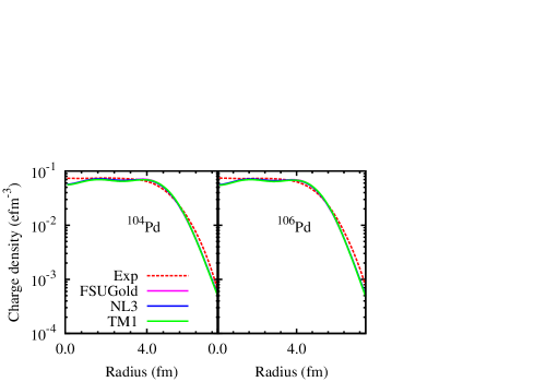
Figure 1: (Color online) Comparison of charge density from our calculation with Fourier- Bessel analysis of experimental electron scattering datade

III.2 Astrophysical S factor and reaction rates

In the present case, our calculations, being more microscopic, are more restricting. In general, phenomenological models are usually fine tuned for nuclei near the stability valley, but not very successful in describing elements near the proton and neutron rich regions. Microscopic models, in contrary, can be extended to the drip line regions and therefore, this method can be used to study the reaction rates of nuclei involved in $p$ process nucleosynthesis network ($\sim$ 2000 nuclei are present in the total $p$ network). However, only a few number of stable $p$ nuclides are available in nature that can be accessed by the experiment and therefore we are restricted to those nuclei for the purpose of comparison .

As a first test of the optical model potential, we have calculated elastic proton scattering at low energies where experimental data are available. As the elastic scattering process involves the same incoming and outgoing channel for the optical model, therefore it is expected to provide the easiest way to constrain various parameters involved in the calculation. Here we are mainly interested in the energy region between 2-8 MeV as the astrophysical important Gamow window lies within this energy range in the concerned mass region. However, scattering experiments are very difficult at such low energies, because the cross sections are extremely small, and hence no experimental data are available. Therefore we have compared the cross sections from our calculations with the lowest energy experimental data available in the literature.

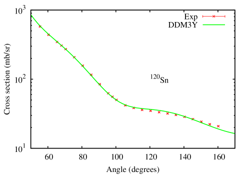
Figure 2: (Color online) Experimental and calculated cross sections for elastic proton scattering at 9.7 MeV proton energy

In figure 2, we present the result of our calculation with DDM3Y folded potential for ¹²⁰Sn with available experimental datadiff . To fit the experimental data, at first, the folded DDM3Y potential is multiplied by factors 0.3 and 0.7 to obtain the real and imaginary parts of the optical potential, respectively. However better fits for individual reactions can be possible by varying different parameters. But if the present calculation has to be extended to an unknown mass region, this approach is clearly inadequate. Therefore, we have refrained from fitting individual reactions. For example, in a previous workclah2 , the real and imaginary part of the potential was multiplied to 0.7 and 0.1 respectively. But beyond that, the same set of parameters was unable to fit the experimental data for $p$ nuclei in mass 80 region, and therefore the real and the imaginary part normalizations were chosen to be 0.81 and 0.15 respectively, in mass 90 regionclah2 . However, there are no sharp boundaries for these mass regions, but for simplicity, we chose it in such a way that a single set of parameters can fit the entire mass region. In this work, we consider A $\sim$ 100-120 region as we can trace the whole region with same set of parameters.

Yet, the astrophysical reaction rates depend on the proper choice of the level density and the E1 gamma strength. Therefore, we have calculated all of our results with microscopic level densities in Hartree-Fock (HF) and Hartree-Fock-Bogoliubov (HFB) methods, calculated for TALYS database by Goriley and Hilairetalys ; gori on the basis of Hartree-Fock calculationsgori1 . We have also compared our results using phenomenological level densities from a constant-temperature Fermi gas model, a back-shifted Fermi gas model, and a generalized superfluid model from TALYS. All these model parameters can be availed from TALYS database. We find that the cross sections are very sensitive to the level density parameters, sometimes by a factor of 20%. We therefore analyzed, in most of the cases, the HF level densities fit the experimental data better in this mass region. Again, for E1 gamma strength functions, results derived from HF + BCS and HFB calculations, available in the TALYS database, are employed. In this case also, the results for HF+BCS calculations describe the experimental data reasonably well and we present our results for that approach only.

We now calculate some $(p,\gamma)$ cross sections relevant to $p$ nuclei in A$\sim$100-120 region where experimental data are available. At such low energies, reaction cross-section varies very rapidly making comparison between theory and experiment rather difficult. Therefore the usual practice in low-energy nuclear reaction is to compare another key observable, viz. the S factor. It can be expressed asclah1

$$S(E)=E\sigma(E)e^{2\pi\eta},$$ (10)

where E is the energy in center of mass frame in keV which factorises out the pre-exponential low energy dependence of reaction cross-section $\sigma(E)$, and $\eta$ indicates the Sommerfeld parameter with

$$2\pi\eta=31.29Z_{p}Z_{t}\sqrt{\frac{\mu}{E}}.$$ (11)

The factor exp$(2\pi\eta)$ is inversely proportional to the transmission probability through the Coulomb barrier with zero angular momentum(s-wave) and therefore removes exponential low energy dependence of $\sigma(E)$. Here $\sigma(E)$ is in barn, $Z_{p}$ and $Z_{t}$ are the charge numbers of the projectile and the target, respectively and $\mu$ is the reduced mass (in amu) of the composite system. This S factor varies much slowly than reaction cross-sections and for this reason, we calculate this quantity and compare it with experimentally obtained values.

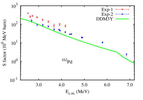
Figure 3: (Color online) S factors from two different microscopic potentials are compared with experimental measurements for ¹⁰²Pd. Here “Exp-1”is the experimental data from referencepd102r1 , “Exp-2”from referencepd102r2 and “DDM3Y”is for the DDM3Y-folded potential.

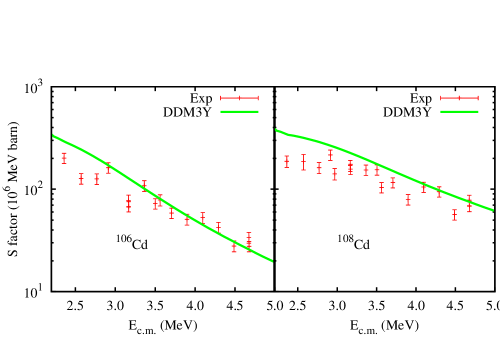
Figure 4: (Color online) S factors extracted from theory compared with experimental measurements for ^106,108Cd. Here “Exp”is the experimental data from referencecdref .

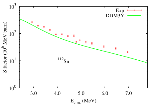
Figure 5: (Color online) S factors extracted from theory compared with experimental measurements for for ¹¹²Sn.

In figures 3-5 we present the results of some of our calculations with folded DDM3Y potential for Pd,Cd and Sn isotopes, respectively, along with the corresponding experimental results. The experimental values for ¹⁰²Pd are from referencepd102r1 (red point) and pd102r2 (green cross), ^106,108Cd from Gy. Gyürky et al. cdref and ¹¹²Sn from reference sn112ref .

In case of ¹⁰²Pd in figure 3, theoretical prediction is in a good agreement, mainly in the low energy regime, with the experimental data from reference pd102r2 but under predicts the data obtained from the referencepd102r1 . In reference pd102r1 , an activation technique was used in which gamma rays from decays of the reaction products were detected off-line by two hyper-pure germanium detectors in a low background environment, whereas in reference pd102r2 , cross-section measurements have been carried out at the cyclotron and Van de Graaff accelerator by irradiation of thin sample layers and subsequent counting of the induced activity. However, we can not comment on the individual merits of these experiments.

In case of ^106,108Cd in figure 4, one can find that the agreement of theory with experimental values are good enough, however there is a slight over prediction of ¹⁰⁸Cd in the low energy regime. In case of ¹¹²Sn in figure 5, our calculation follows the experiment in a fairly good fashion.

The success of this microscopic optical potential (DDM3Y interaction folded with FSUGold density)in reproducing S factor data for the above $p$ nuclei leads us to calculate reaction rates of some astrophysically important reactions. In figure 6, we compare $(p,\gamma)$ reaction rates for some important $p$ nuclei with NONSMOKER ratesrate . Again in figure 7, reaction rates for charge exchange reactions $(p,n)$ for some nuclei, however not astrophysically significant enough, in this mass region are compared with existing NONSMOKER calculations. One can see that the present calculation is very similar to the NONSMOKER values in almost all cases. Therefore, it is expected that all the results can also be reproduced with commonly used NONSMOKER rates.

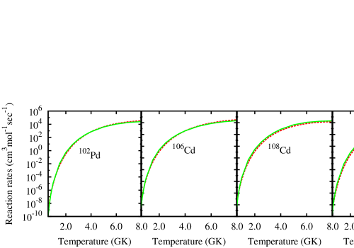
Figure 6: (Color online) Astrophysical reaction rates for $(p,\gamma)$ reactions of some important $p$ nuclei compared with NONSMOKER ratesrate . Here Green Continuous line: Present calculation, Red Dotted line: NONSMOKER calculation.

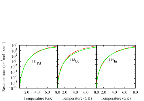
Figure 7: (Color online) Astrophysical reaction rates for $(p,n)$ reactions compared with NONSMOKER ratesrate . Here Green Continuous line: Present calculation, Red Dotted line: NONSMOKER calculation.

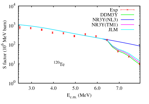
Figure 8: (Color online) S factors extracted from our calculations compared with experimental measurements for ¹²⁰Te. Here “Exp”is the experimental data from referencete120ref . For other details, see the text.

In the rest of the present manuscript, we mainly concentrate on the effects of optical potentials obtained by folding nonlinear interactions from RMF. In figure 8, S factors for ¹²⁰Te obtained from NR3Y(NL3) and NR3Y(TM1) potentials are compared with the experimental data taken from referencete120ref . The S- factor with DDM3Y interaction folded with FSUGold density is also given for comparison. For better understanding, we have associated the result from JLMjlm ; jlm2 potential also, which can be found on TALYS code.

One can see that our calculation with folded DDM3Y potential shows a very nice agreement with experimental values throughout the energy range. The result from JLM interaction also agrees with the experiment. In contrary, in case of NR3Y(NL3)folded potential, there is a wide deviation of the theory with experimental data after 6 MeV whereas the TM1 folded potential NR3Y(TM1) shows a decrease in S factor value around 6 MeV energy unlike the NR3Y(NL3)case.

The rapid drop of S factor values with increasing energy actually takes place due to the increasing contribution of higher angular momentum channels (l$>$0). Therefore, if the center of mass energy E_c.m. becomes larger than the Coulomb barrier for a specific set of nucleon-nucleus reaction (E${}_{c.m.}>$E_c), as a result the S factor will decrease rapidly with the growth of energy (E_c.m.)sf . In the next subsection, we illustrate this physics in detail and show how this phenomenon is associated with different form of potentials.

III.3 Optical potentials and effects for nonlinearity

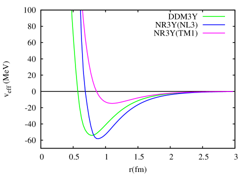
Figure 9: (Color online) Effective interaction potential for ${}^{120}Te$.

We now interpret the above results (for example, see figure 8) with the microscopic potentials obtained from different $NN$ interactions. In figure 9, the effective $NN$ interaction potentials (in MeV) are plotted with the radius r(fm) for ¹²⁰Te. The DDM3Y interaction, being dependent on the density, is different for different elements of the periodic table, whereas in contrary, other interactions remain unaltered for different elements. In figure 9 different forms of $NN$ interactions are given. We find that the curves from DDM3Y and NR3Y(NL3) interactions generated from two different formalisms show almost similar trend which makes us believe that this nonlinear form of the $NN$ interaction can also be used to obtain the microscopic optical potential.

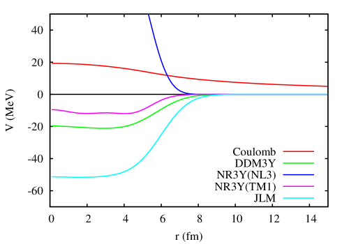
Figure 10: (Color online) Real central part of folded potentials and Coulomb potential for 7 MeV proton(Lab) incident on ¹²⁰Te

A graphical representation of microscopic potentials for ¹²⁰Te after folding the interactions is represented in figure 10. Here the real central part of the optical potential is plotted with the radius. In the figure, one can see that the DDM3Y folded potential provides an attractive potential similar to the real part of the JLM potential, whereas in case of NR3Y(NL3) folded potential, the repulsive part overpowers the attractive part, as well as the Coulomb part of the potential. As a result, the resultant repulsive barrier becomes greater than the Coulomb barrier almost upto a range for a nuclear reaction to occur. Therefore the penetrability of the higher angular momentum channels get reduced and as a obvious consequence, the desirable sharp drop in S factor (figure 8) values has not been achieved. In case of TM1 folded potential, we can see that the effective contribution of the optical potential is attractive in nature similar to the DDM3Y and JLM potentials and therefore, the Coulomb energy serves as the only repulsive barrier. As a result the penetration probability for higher angular momentum channels becomes higher than that of the NR3Y(NL3)case. This reason is replicated as a drop of S factor values at higher energies in figure 8. In case of the imaginary part of the potential, the curves follow exactly the similar trend as that of the real part, i.e., apart from NR3Y(NL3) potential, rest of them gives attractive contribution. One can explain the above scenario from the numerical value of the nonlinear coupling constant g₃(TM1 parameter set), as given in Table 1, which is much less than that of the NL3 parameter set. Therefore it can be understood that with decreasing values of the nonlinear coupling constants g₂ and g₃, the repulsive component of the optical potential also gets reduced and one point is attained when only the effect of Coulomb barrier remains as a dominating repulsive contributor and we will get patterns like JLM, TM1, DDM3Y as shown in figure 10 and we can find the expected drop of S factor values at higher energies due to the opening of higher angular momentum channels. So from the above observations we can comment that there should be an upper cut-off for the coupling constant values of the nonlinear components.

IV Summary and Discussion

To summarize, cross section for low energy $(p,\gamma)$ reactions for a number of $p$ nuclei in A$\sim$100-120 region have been calculated using microscopic optical model potential with the Hauser Feshbach reaction code TALYS. Mainly, microscopic potential is obtained by folding DDM3Y interaction with densities from RMF approach. Astrophysical reaction rates for $(p,\gamma)$ and $(p,n)$ reactions are compared with standard NONSMOKER results. Finally, the effect of microscopic optical potential obtained by folding nonlinear NR3Y(NL3) and NR3Y(TM1) interactions with corresponding RMF densities are employed to fit the experimental S factor data for ¹²⁰Te. The reason of the deviation of theoretical prediction with nonlinear NR3Y(NL3) potential from experiment at higher energies has been discussed and finally we made a comment on magnitude of the coupling terms of the nonlinear components that an upper cut-off value for $g_{2}$ and $g_{3}$ should be fixed to get proper repulsive component of the $NN$ interaction.

References

- (1) C. Illiadis, Nuclear Physics of the Stars (Wiley-VCH Verlag GmbH, Weinheim, 2007).
- (2) M. Arnould and S. Goriely, Phys. Rep. 384 (2003) 1.
- (3) T. Rauscher and F.K. Thielemann, At. Data. Nucl. Data. Tables 75 (2000) 1; 79 (2000) 47.
- (4) G. Gangopadhyay, Phys. Rev. C 82 (2010) 027603.
- (5) C. Lahiri and G. Gangopadhyay, Eur. Phys. J. A 47 (2011) 87.
- (6) C. Lahiri and G. Gangopadhyay, Phys. Rev. C 84 (2011) 057601.
- (7) C. Lahiri and G. Gangopadhyay, Phys. Rev. C 86 (2012) 047601.
- (8) S. Datta, D. Chakraborty, G. Gangopadhyay, and A. Bhattacharyya, Phys. Rev. C 91 (2015) 025804.
- (9) D. Chakraborty, S. Dutta, G. Gangopadhyay, and A. Bhattacharyya, Phys. Rev. C 91 (2015) 057602.
- (10) P.-G. Reinhard, Z. Phys. A - Atomic Nuclei 329 (1988) 257.
- (11) B. B. Sahu, S. K. Singh, M. Bhuyan, S. K. Biswal and S. K. Patra, Phys. Rev. C 89 (2014) 034614.
- (12) J. D. Walecka, Annals of physics 83 (1974) 491 .
- (13) P. Ring, Prog. Part. Nucl. 37 (1996) 193.
- (14) Michael Bender, Paul-Henri Heenen, and Paul-Gerhard Reinhard, Rev. of Mod. Phys. 75(2003) 121 .
- (15) B. D. Serot and J. D. Walecka, Adv. Nucl. Phys 16 (1986) 1.
- (16) L. D. Miller and A. E. S. Green, Phys. Rev. C 5(1972) 241 .
- (17) P. -G. Reinhard and M. Bendev, Extended Density Functionals in Nuclear Structure Physics Lecture Notes in Physics 641 (2004) 249.
- (18) Bir Bikram Sing, M. Bhuyan, S. K. Patra and Raj K Gupta, J. Phys. G: Nucl. Part. Phys. 39 (2012) 069501.
- (19) B.G. Todd-Rutel and J. Piekarewicz, Phys. Rev. Lett. 95 (2005) 122501.
- (20) G. Bertsch, J. Borysowicz, H. McManus, and W.G. Love, Nucl. Phys. A 284(1977) 399 ; W.D. Myers, Nucl. Phys. A 204 (1973) 465 ; D.N. Basu, J. Phys. G: Nucl. Part. Phys. 30 (2004) B7.
- (21) G. A. Lalazissis, J. König, P. Ring, Phys. Rev. C 55 (1997) 540.
- (22) Y. Sugahara and H. Toki, Nucl. Phys. A 579 (1994) 557.
- (23) R.R. Scheerbaum, Nucl. Phys. 257 (1976) 77.
- (24) A.J. Koning et al., Proc. Int. Conf. Nucl. Data Science Tech., April 22-27, 2007, Nice, France, EDP Sciences, (2008) p. 211.
- (25) J.-P. Jeukenne, A. Lejeune, and C. Mahaux, Phys. Rev. C 16 (1977) 80.
- (26) E. Bauge, J. P. Delaroche, and M. Girod, Phys. Rev. C 63 (2001) 024607.
- (27) S. K. Patra, R. N. Panda, P. Arumugam, and R. K. Gupta, Phys. Rev. C 80 (2009) 064602.
- (28) M. Wang, G. Audi, A.H. Wapstra, F.G. Kondev, M. MacCormick, X. Xu, and B. Pfeiffer, Chinese Phys. C 36 (2014) 1603.
- (29) I. Angeli, K.P. Marinova, At. Data. Nucl. Data. Tables 99 (2013) 69.
- (30) H. De Vries, C. W. De Jager, and C. De Vries, At. Data. Nucl. Data. Tables 36 (1987) 495.
- (31) G. W. Greenlees, C. H. Poppe, J. A. Sievers, and D. L. Watson, Phys. Rev. C 3 (1971) 1231.
- (32) S. Goriely, S. Hilaire and A.J. Koning, Phys. Rev. C 78 (2008) 064307.
- (33) S. Goriely, F. Tondeur, J.M. Pearson, At. Data. Nucl. Data. Tables 77 (2001) 311.
- (34) N. Özkan et al. , Nucl. Phys. A 710 (2002) 469.
- (35) I. Dillmann et al. , Phys. Rev. C 84 (2011) 015802.
- (36) Gy. Gyürky et al. , J. Phys. G: Nucl. Part. Phys. 34 (2007) 817.
- (37) F.R. Chloupek et al. , Nucl. Phys. A 652 (1999) 391.
- (38) R. T. Güray et al. , Phys. Rev. C 80 (2009) 035804.
- (39) D. G. Yakovlev, M. Beard, L. R. Gasques and M. Wiescher, Phys. Rev. C 82 (2010) 044609.