A proof to Biswas-Mitra-Bhattacharyya conjecture for ideal quantum gas trapped under generic power law potential $U=\sum_{i=1}^{d}c_{i}|\frac{x_{i}}{a_{i}}|^{n_{i}}$ in $d$ dimension

Abstract

The well known relation for ideal classical gas $\Delta\epsilon^{2}=kT^{2}C_{V}$ which does not remain valid for quantum system is revisited. A new connection is established between energy fluctuation and specific heat for quantum gases, valid in the classical limit and the degenerate quantum regime as well. Most importantly the proposed Biswas-Mitra-Bhattacharyya (BMB) conjecture (Biswas $et.$ $al.$, J. Stat. Mech. P03013, 2015.)[1] relating hump in energy fluctuation and discontinuity of specific heat is proved and precised in this manuscript.

1 Introduction

An increasing attraction towards the subject of quantum gases is observed, after it was possible to create BEC in magnetically trapped alkali gases[2, 3, 4] as well as experimental confirmation of Fermi degeneracy[5]. Different theoretical and experimental studies analysing the effects of temperature dependence of energy and specific heat of ultracold Fermi gases[5, 6, 7], momentum distribution for harmonically trapped quantum gas[8, 9], temperature dependence of the chemical potential[10], critical number of particles for the collapse of attractively interacting Bose gas[11], Casimir effect[12, 13], equivalence of Bose and Fermi system[14, 15], q deformed systems[16, 17] have already been reported. Although a lot of theoretical studies[18, 19, 20, 21, 22, 23, 24, 25] are done on quantum gases trapped under generic power law potential, none of these contained detailed discussion on energy fluctuation of trapped quantum gases, until the recent paper of Biswas et. al. [1]. In the case of ideal classical gas, specific heat $C_{V}$ is regarded as energy fluctuation $\Delta\epsilon^{2}$ as the $\Delta\epsilon^{2}$ is related to $C_{V}$ as, $\Delta\epsilon^{2}=kT^{2}C_{V}$. But this relation becomes invalid for both types of quantum gases (Bose and Fermi) in the quantum degenerate regime for free quantum gases[1]. Biswas $et.$ $al.$[1] have conjectured (BMB conjecture) a relation between the discontinuity of $C_{V}$ and energy fluctuation. According to the BMB conjecture, the appearance of a hump in $\frac{\Delta\epsilon^{2}}{kT^{2}}$ over its classical limit may indicate a discontinuity of $C_{V}$. They have shown this to be true for free and harmonically trapped Bose gases[1]. They have also mentioned without proving that the the inverse of this statement may not always be true. But this conjecture is yet to be proven for any quantum system trapped under generic power law potential in arbitrary dimension and is an open problem. In this manuscript, we have proved and precised BMB conjecture for ideal quantum gases trapped under generic power law potential, $U=\sum_{i=1}^{d}c_{i}|\frac{x_{i}}{a_{i}}|^{n_{i}}$ in $d$ dimension. Thus, in principle one can reconstruct the results Shyamal $et.$ $al.$, choosing all $n_{i}=2$ for harmonically trapped system and all $n_{i}=\infty$ for free systems. Beside this, a relation is established between $C_{V}$ and ${\Delta\epsilon^{2}}$ which is valid not only in the classical limit but in the quantum limit as well.

The manuscript is organized in the following way. In section 2, we have determined the grand potential in an unified way for both types of quantum gases, from which we are able to calculate the quantities such as $C_{V}$ and $\Delta\epsilon^{2}$. In the next section we elaborate two theorems which eventually guide us to prove the conjecture. Results are discussed in section 4 and the paper is concluded in section 5.

2 Grand potential, specific heat and energy fluctuations

For a quantum gas, the average number of particles occupying the $i$-th eigenstate and the grand potential , are given by

$$\bar{n}_{i} = \frac{1}{z^{-1}e^{\beta\epsilon_{i}}-a}$$ (1)

and,

$$q = \frac{1}{a}\sum_{\epsilon}ln(1+aze^{-\beta\epsilon})$$ (2)

where, $a=1(-1)$ stands for Bose system (Fermi system) and $z$ is fugacity. Let us consider an ideal quantum system trapped in a generic power law potential in $d$ dimensional space with a single particle Hamiltonian of the form,

$$\epsilon(p,x_{i})=bp^{l}+\sum_{i=1}^{d}c_{i}|\frac{x_{i}}{a_{i}}|^{n_{i}}$$ (3)

where, $b,$ $l,$ $a_{i}$, $c_{i}$, $n_{i}$ are all positive constants, $p$ is the momentum and $x_{i}$ is the $i$ th component of coordinate of a particle. Here, $c_{i}$, $a_{i}$, $n_{i}$ determines the depth and confinement power of the potential and $l$ being the kinematic parameter and $x_{i}<a_{i}$. As $|\frac{x_{i}}{a_{i}}|<1$, the potential term goes to zero as all $n_{i}\longrightarrow\infty$. Using $l=2$, $b=\frac{1}{2m}$ one can get the energy spectrum of the hamiltonian used in the literatures [19, 20, 21, 22]. If one uses $l=1$ and $b=c$ one finds the hamiltonian of massless systems such as photons[20].

The density of states for such system is [18, 25],

$$\rho(\epsilon)=C(b,V_{d}^{\prime})\epsilon^{\chi-1}$$ (4)

where, $C(b,V_{d}^{\prime})$ is a constant depending on effective volume $V_{d}^{\prime}$[14]. For the detail derivation of density of states see Ref. [25]. Now, replacing the sum by integral we obtain the grand potential,

$$q=q_{0}+\frac{V_{d}^{\prime}}{\lambda^{\prime d}}Li_{\chi+1}(\sigma)$$ (5)

Note, $Li_{q}(m)$ is known as polylog function in the literature whose integral representation for $Re(m)<1$ is[15]

$$Li_{q}(m)=\frac{1}{\Gamma(q)}\int_{0}^{m}[\ln(\frac{m}{\eta})]^{q-1}\frac{d\eta}{1-\eta},$$ (6)

$$q_{o}=\frac{1}{a}\ln(1+az)$$ (7)

It is a real valued function if $m\in\mathbb{R}$ and $-\infty<m<1$. Also, the effective volume $V_{d}^{\prime}$, effective thermal wavelength $\lambda_{d}^{\prime}$ along with $\chi$ and $\sigma$ are defined as,

$$V_{d}^{\prime} = V_{d}\prod_{i=1}^{d}(\frac{kT}{c_{i}})^{1/n_{i}}\Gamma(\frac{1}{n_{i}}+1)$$ (8)

$$\lambda^{\prime} = \frac{hb^{\frac{1}{l}}}{\pi^{\frac{1}{2}}(kT)^{\frac{1}{l}}}[\frac{d/2+1}{d/l+1}]^{1/d}$$ (9)

$$\chi =\frac{d}{l}+\sum_{i=1}^{d}\frac{1}{n_{i}}$$ (10)

$$\sigma =\left\{\begin{array}[]{lr}-z&,\text{Fermi system}\\ z&,\text{Bose system}\end{array}\right.$$ (13)

The detail idea of effective thermal wavelength and effective volume for trapped quantum gases can be found in[23, 24, 25, 26]. But note, when $l=2$ and $b=\frac{1}{2m}$ from Eq. (8) we get $\lambda_{0}=\frac{h}{(2\pi mkT)^{1/2}}$, which is the thermal wavelength of nonrelativistic massive fermions as well as massive bosons. However, it should be noted that, when $l\neq 2$, $\lambda^{\prime}$ then depends on dimension. With $d=3$ and $d=2$, thermal wavelength of photons (boson) and neutrinos (fermion) are respectively[19] $\frac{hc}{2\pi^{1/2}kT}$ and $\frac{hc}{(2\pi)^{1/2}kT}$ which can be obtained from from Eq. (9) by choosing $b=c$, where $c$ being the velocity of light. But one needs to consider the effects of antiparticles to calculate the thermodynamic quantities of ultrarelativistic quantum gas[27]. So, one can reproduce the thermal wavelength of both massive and massless particles from the definition of effective thermal wavelength $\lambda^{\prime}$ with more general energy spectrum. It is also seen that the effective volume $V_{d}^{\prime}$ is a very salient feature of the trapped system as this allows us to treat the trapped quantum gases[14, 23, 24, 25] to be treated as a free one. Difference between $V_{d}^{\prime}$ and $V_{d}$ is that, the former depends on temperature and power law exponent while the latter does not. But as all $n_{i}\longrightarrow\infty$, $V_{d}^{\prime}$ approaches $V_{d}$. The great benefit of evaluating $V_{d}^{\prime}$ and $\lambda^{\prime}$ is that they enable us to write all of the thermodynamic functions of the trapped quantum system to be expressed in a compact form similar to those of a free quantum gas[14, 23]. It is well known that the Bose and Fermi functions do represent thermodynamics of Bose and Fermi system and can be written in terms of Polylogarithmic functions,

$$Li_{l}(z)=g_{l}(z)=\frac{1}{\Gamma(l)}\int_{0}^{\infty}dx\frac{x^{l-1}}{z^{-1}e^{x}-1}$$ (14)

$$-Li_{l}(-z)=f_{l}(z)=\frac{1}{\Gamma(l)}\int_{0}^{\infty}dx\frac{x^{l-1}}{z^{-1}e^{x}+1}$$ (15)

Point to note, as $z\rightarrow 1$, the Bose function $g_{\chi}(z)$ approaches $\zeta(\chi)$, for $\chi>1$[19]. From the grand potential we can now determine,

$$E=-(\frac{\partial q}{\partial\beta})_{z,V_{d}^{\prime}}=NkT\chi\frac{Li_{\chi+1}(\sigma)}{Li_{\chi}(\sigma)}$$ (16)

$$C_{V}=(\frac{\partial U}{\partial T})_{N,V_{d}^{\prime}}=Nk[\chi(\chi+1)\frac{Li_{\chi+1}(\sigma)}{Li_{\chi}(\sigma)}-\chi^{2}\frac{Li_{\chi}(\sigma)}{Li_{\chi-1}(\sigma)}]$$ (17)

In the classical limit of quantum gases, $C_{V}$ equals to $Nk\chi$. Now, the energy fluctuation

$$\Delta\epsilon^{2} = \bar{\epsilon^{2}}-\bar{\epsilon}^{2}=\sum_{i}\bar{n}_{i}\epsilon_{i}^{2}-(\sum_{i}\bar{n}_{i}\epsilon_{i})^{2}=\int d\epsilon\rho(\epsilon)\epsilon^{2}n(\epsilon)-(\int d\epsilon\rho(\epsilon)\epsilon n(\epsilon))^{2}$$ (18)

$$= (kT)^{2}[\chi(\chi+1)\frac{Li_{\chi+2}(\sigma)}{Li_{\chi}(\sigma)}-\chi^{2}\frac{Li_{\chi+1}^{2}(\sigma)}{Li_{\chi}^{2}(\sigma)}]$$

So, it is clear from Eq. (15) and (16) that, $\Delta\epsilon^{2}\neq kT^{2}C_{V}$. But it is valid in the classical limit as $z\rightarrow 0$, Eq. (15) and (16) deptics,

$$\Delta\epsilon^{2}=kT^{2}C_{V}=N\chi(kT)^{2}$$ (19)

But we can establish such a relation valid within the whole temperature range. Note,

$$\Delta\epsilon^{2}=\bar{\epsilon^{2}}-\bar{\epsilon}^{2} = (\frac{\partial E}{\partial\beta})_{{}_{z,V_{d}^{\prime}}}=kT^{2}(\frac{\partial E}{\partial T})_{{}_{z,V_{d}^{\prime}}}=kT^{2}(\frac{\partial E}{\partial T})_{{}_{N,V_{d}^{\prime}}}+kT^{2}(\frac{\partial E}{\partial N})_{{}_{T,V_{d}^{\prime}}}(\frac{\partial N}{\partial T})_{{}_{z,V_{d}^{\prime}}}$$ (20)

$$= kT^{2}C_{V}+kT(\frac{\partial E}{\partial N})_{{}_{T,V_{d}^{\prime}}}(\frac{\partial E}{\partial\mu})_{{}_{T,V_{d}^{\prime}}}$$

where, in the last line we have used $\frac{1}{T}(\frac{\partial E}{\partial\mu})_{{}_{T,V_{d}^{\prime}}}=(\frac{\partial N}{\partial T})_{{}_{z,V_{d}^{\prime}}}$[19]. In the high temperature limit the second term of Eq. (18) becomes zero and Eq. (18) coincides with Eq. (17). It can be easily justified that equation (18) is valid not only in the classical limit but also in the quantum degenerate regime.

Point to note that expression of $C_{V}$ and $\Delta\epsilon^{2}$ represents both Bose and Fermi system in a unified approach. In the case of Fermi system,

$$C_{V}=Nk[\chi(\chi+1)\frac{f_{\chi+1}(z)}{f_{\chi}(z)}-\chi^{2}\frac{f_{\chi}(z)}{f_{\chi-1}(z)}]$$ (21)

$$\Delta\epsilon^{2}=(kT)^{2}[\chi(\chi+1)\frac{f_{\chi+2}(z)}{f_{\chi}(z)}-\chi^{2}\frac{f_{\chi+1}^{2}(z)}{f_{\chi}^{2}(z)}]$$ (22)

The above equations coincides exactly with the results of Ref. [1] appropriate choice of $n_{i}$ and $d$. Writing the expressions for Bose system (per particle),

$$C_{V}=\left\{\begin{array}[]{lr}k[\chi(\chi+1)\frac{\nu^{\prime}}{\lambda^{\prime D}}g_{\chi+1}(z)-\chi^{2}\frac{g_{\chi}(z)}{g_{\chi-1}(z)}]&,T>T_{c}\\ k\chi(\chi+1)\frac{\nu^{\prime}}{\lambda^{\prime D}}\zeta(\chi+1)&,T\leq T_{c}\end{array}\right.$$ (25)

$$\Delta\epsilon^{2}=\left\{\begin{array}[]{lr}(kT)^{2}[\chi(\chi+1)\frac{g_{\chi+2}(z)}{g_{\chi}(z)}-\chi^{2}\frac{g_{\chi+1}^{2}(z)}{g_{\chi}^{2}(z)}]&,T>T_{c}\\ (kT)^{2}[A_{1}(\frac{T}{T_{C}})^{\chi}-A_{2}(\frac{T}{T_{C}})^{2\chi}]&,T\leq T_{c}\end{array}\right.$$ (28)

Here $T_{C}$ denotes critical temperature and, $A_{1}$ and $A_{2}$ are defined as,

$$A_{1} = \chi(\chi+1)\frac{\zeta(\chi+2)}{\zeta(\chi)}$$ (29)

$$A_{2} = [\chi\frac{\zeta(\chi+1)}{\zeta(\chi)}]^{2}$$ (30)

Eq. (22) agrees with the expressions for free and harmonically trapped Bose system in three dimensional space[1]. It is noteworthy that, for both types of trapped quantum gases, $C_{V}$ approaches its classical value $\chi NK$ [28].

3 Theorems regarding $C_{V}$ and $\Delta\epsilon^{2}$ of Bose gas

In this section we present the necessary theorems to prove the conjecture. As it was shown by Shyamal $et.$ $al.$ that a hump does exist in ${\Delta\epsilon^{2}}/{kT^{2}C_{V}^{{}^{cl}}}$ in the condensed phase for harmonically trapped Bose gas, we need to find a general criteria to locate a hump in ${\Delta\epsilon^{2}}/{kT^{2}C_{V}^{{}^{cl}}}$ over its classical limit in arbitrary dimension with any trapping potential. As there is no condensed phase in ideal Fermi gas trapped under potential[29], this theorem bears no significance for them.

Theorem 4.1: Let an ideal Bose gas in an external potential, $U=\sum_{i=1}^{d}c_{i}|\frac{x_{i}}{a_{i}}|^{n_{i}}$. A hump will exist in the condensed phase in ${\Delta\epsilon^{2}}/{kT^{2}C_{V}^{{}^{cl}}}$ over the classical limit if,

$$\chi<\frac{A_{1}^{2}}{4A_{2}}=\gamma(\chi)$$

$$\Rightarrow \chi\geqslant 2.3$$

Proof:

Re-writing Eq. (22) in the condensed phase,

$$\frac{\Delta\epsilon^{2}}{(kT)^{2}}=f(\tau)=A_{1}\tau^{\chi}-A_{2}\tau^{2\chi}$$

$$\Rightarrow f^{\prime}(\tau)=\frac{\partial f}{\partial\tau}=A_{1}\chi\tau^{\chi-1}-2A_{2}\chi\tau^{2\chi-1}$$ (31)

The condition for maximum,

$$f^{\prime}(\tau)\bigg{|}_{\tau=\tau_{0}}=0$$

$$\Rightarrow\tau_{0}^{\chi}=\frac{A_{1}}{2A_{2}}$$ (32)

The hump will be over its classical limit if,

$$f(\tau)\bigg{|}_{\tau=\tau_{0}}>\chi$$

$$\Rightarrow A_{1}\tau_{0}^{\chi}-A_{2}\tau_{0}^{2\chi}>\chi$$

$$\Rightarrow \chi<\gamma(\chi)=\frac{A_{1}^{2}}{4A_{2}}$$ (33)

From the Table 1, one can conclude relation (27) will be maintained (a hump will exist in the condensed phase over the classical limit) when,

$$\chi\geqslant 2.3$$ (34)

Table 1: Listed values of $\gamma(\chi)$, generated using Mathematica (Correct upto four decimal points).

$\chi$	$\gamma(\chi)$
1.3	0.8553
1.4	0.9756
1.5	1.1022
1.6	1.2350
1.7	1.3736
1.8	1.5181
1.9	1.6683
2.0	1.8240
2.1	1.9853
2.2	2.1519
2.3	2.3239
2.4	2.5010
2.5	2.6834
2.6	2.8709

Theorem 4.2: Let an ideal Bose gas in an external potential, $U=\sum_{i=1}^{d}c_{i}|\frac{x_{i}}{a_{i}}|^{n_{i}}$,

(i) $C_{V}$ will be discontinuous at $T=T_{c}$ if,

$$\chi=\frac{d}{l}+\sum_{i=1}^{d}\frac{1}{n_{i}}>2$$

.
(ii) And the difference between the heat capacities at constant volume, at $T=T_{c}$ as

$$\Delta C_{V}\mid_{{}_{T=T_{c}}}=C_{V}\mid_{{}_{T_{c}^{-}}}-C_{V}\mid_{{}_{T_{c}^{+}}}=Nk\chi^{2}\frac{\zeta(\chi)}{\zeta(\chi-1)}$$

Proof:

As $T\rightarrow T_{c}$, $z\rightarrow 1$ and $\eta\rightarrow 0$, where $\eta=-\ln z$. For $T\rightarrow T_{c}^{+}$,

$$C_{V}(T_{C}^{+}) =Nk[\chi(\chi+1)\frac{\nu^{\prime}}{\lambda^{\prime D}}g_{\chi+1}(z)|_{{}_{z\rightarrow 1}}-\chi^{2}\frac{g_{\chi}(z)}{g_{\chi-1}(z)}|_{{}_{z\rightarrow 1}}]$$ (35)

$$=Nk[\chi(\chi+1)\frac{\nu^{\prime}}{\lambda^{\prime D}}\zeta({\chi+1})-\chi^{2}\frac{\zeta({\chi})}{g_{\chi-1}(z)}|_{{}_{z\rightarrow 1}}]\$$

As the denominator of the second term of the right hand side contains $g_{\chi-1}(z)$, we can not simply substitute it with zeta function as $z\rightarrow 1$. So, using the representation of Bose function by Robinson[30],

$$g_{\chi}(e^{-\eta})=\frac{\Gamma(1-\chi)}{\eta^{1-\chi}}+\sum_{i=0}^{\infty}\frac{(-1)^{i}}{i!}\zeta(\chi-i)\eta^{i}$$ (36)

we get from the above,

$$C_{V}(T_{C}^{+})=Nk[\chi(\chi+1)\frac{\nu^{\prime}}{\lambda^{\prime d}}\zeta({\chi+1})-\chi^{2}\frac{\zeta({\chi})}{\Gamma(2-\chi)}\eta^{2-\chi}\mid_{\eta\rightarrow 0}]$$ (37)

On the other hand

$$C_{V}(T_{C}^{-})=Nk[\chi(\chi+1)\frac{\nu^{\prime}}{\lambda^{\prime d}}\zeta({\chi+1})$$ (38)

Taking the difference between $C_{V}(T_{C}^{+})$ and $C_{V}(T_{C}^{-})$, we get,

$$\Delta C_{V}\mid_{{}_{T=T_{c}}}=\chi^{2}\frac{\zeta({\chi})}{\Gamma(2-\chi)}\eta^{2-\chi}\mid_{\eta\rightarrow 0}$$ (39)

Which dictates, $\Delta C_{V}\mid_{{}_{T=T_{c}}}$ will be non zero for $\chi>2$. So, $C_{V}$ will be discontinuous when $\chi>2$ and thus completing first part of the theorem.

As, $\chi$ should be greater than two for $\Delta C_{V}$ at $T=T_{C}$ to be non-zero, we can re-write equation (21), by substituting $g_{\chi-1}(z)$ by zeta function.

$$C_{V}(T_{C}^{+})=Nk[\chi(\chi+1)\frac{\nu^{\prime}}{\lambda^{\prime D}}\zeta({\chi+1})-\chi^{2}\frac{\zeta({\chi})}{\zeta({\chi-1})}]$$ (40)

From Eq. (32) and (34) we can write.

$$\Delta C_{V}\mid_{{}_{T=T_{c}}}=C_{V}\mid_{{}_{T_{c}^{-}}}-C_{V}\mid_{{}_{T_{c}^{+}}}=Nk\chi^{2}\frac{\zeta(\chi)}{\zeta(\chi-1)}$$ (41)

Note that, the same result is also derived by Yan et. al. for Bose gas trapped in symmetric power law potential[25].

Now, based on the above two theorems we can come to the conclusion. We have seen, a hump will exist in ${\Delta\epsilon^{2}}/{kT^{2}C_{V}^{{}^{cl}}}$ over the classical limit when $\chi\geqslant 2.3$ and $C_{V}$ will be discontinuous while $\chi>2$. Therefore the existence of hump in ${\Delta\epsilon^{2}}/{kT^{2}C_{V}^{{}^{cl}}}$ over the classical limit automatically ensures discontinuity in $C_{V}$. But a discontinuity in $C_{V}$ does not imply a hump in ${\Delta\epsilon^{2}}/{kT^{2}C_{V}^{{}^{cl}}}$ over the classical limit when the value of $\chi$ is in between, $2<\chi<2.3$ and thus, proving the conjecture.

4 Results and Discussion

In this section we discuss energy fluctuation and specific heat in detail and check the prediction of the above theorems. We have illustrated in this paper how specific heat can differ from the energy fluctuation for the entire range of temperature. It is important to note that the difference between the probabilities of the classical and the quantum gas arises essentially from the nonzero fugacity of the quantum gas.

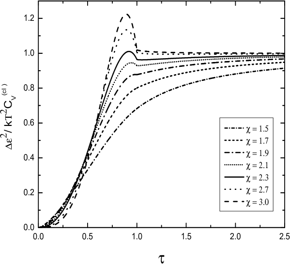
Figure 1: Energy fluctuation ideal trapped Bose gas as a function of $\tau=\frac{T}{T_{C}}$, with different power law potentials.

Table 2: Status of energy fluctuation and specific heat of Bose system trapped under generic power law potential.

Range of $\chi$	Hump over classical limit in ${\Delta\epsilon^{2}}/{kT^{2}C_{V}^{cl}}$	Discontinuity of $C_{V}$
$0<\chi\leqslant 2$	no hump over classical limit	continuous
$2<\chi<2.3$	no hump over classical limit	discontinuous
$\chi\geqslant 2.3$	hump over classical limit	discontinuous

In case of trapped quantum gases all thermodynamic quantities are expressed by polylogarithmic functions depending on fugacity and $\chi$. Thus apart from fugacity, the value of $\chi$ bears the signature of difference between different quantum systems. And as seen from the theorems the value of $\chi$ dictates whether there will be a hump over the classical limit as well as the discontinuity of $C_{V}$. In figure 1 we have described the influence of different power law potentials on energy fluctuation of Bose system. It is clearly seen that, the ${\Delta\epsilon^{2}}/{kT^{2}C_{V}^{cl}}$ has a hump way over its classical limit when $\chi>2.3$. At $\chi=2.3$. the hump is just over its classical limit. There is no hump over the classical limit when $\chi<2.3$, All of these are in accordance with theorem 4.1. It is also noticed that, results in Shamyal et. al. [1] are also in agreement with the theorem. In their manuscript they found a hump over the classical limit in three dimensional harmonically trapped Bose system where $\chi=\frac{3}{2}+\frac{3}{2}=3>2.3$. Although they did find a hump in two dimensional harmonically trapped Bose system but this hump was below the classical limit. In this case, $\chi=\frac{2}{2}+\frac{2}{2}=2<2.3$ $i.e.$, no hump over the classical limit. Therefore, it can be said that the theorem 4.1 can perfectly determine whether the humps will be below or above the classical limit.

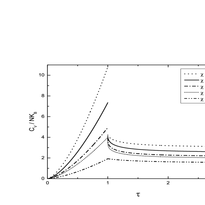
Figure 2: Specific heat of ideal trapped Bose gas as a function of $\tau=\frac{T}{T_{C}}$, with different power law potentials.

Now figure 2 illustrates $C_{V}$ of Bose system with different trapping potentials. It is seen from the figure that, $C_{V}$ is continuous when $\chi\leqslant 2$ and it becomes discontinuous when $\chi>2$, in agreement with theorem 4.2. Now, as $\chi\geqslant 2.3$ denotes a hump in ${\Delta\epsilon^{2}}/{kT^{2}C_{V}^{cl}}$ over its classical limit, this automatically depicts discontinuity in $C_{V}$. Thus, we can conclude that the appearance of a hump in ${\Delta\epsilon^{2}}/{kT^{2}C_{V}^{cl}}$ over its classical limit does indicate a discontinuity in $C_{V}$ but a discontinuity in $C_{V}$ does not conclude the appearance of a hump in ${\Delta\epsilon^{2}}/{kT^{2}C_{V}^{cl}}$ over its classical limit because discontinuity in $C_{V}$ may arise even if $2<\chi<2.3$ but no hump in $\Delta\epsilon^{2}$ will exist in this interval of $\chi$. On the other hand, $\chi\geqslant 2.3$ will denote a discontinuity in $C_{V}$ as well as the appearance of a hump in ${\Delta\epsilon^{2}}/{kT^{2}C_{V}^{cl}}$ over its classical limit (see table 2).

5 Conclusion

In this manuscript we have restricted our study in the case of ideal quantum gases trapped under generic power law potential and proved the BMB conjecture for these types of systems. Point to note, as no hump in $\Delta\epsilon^{2}$ or no discontinuity in $C_{V}$ is noticed in ideal Fermi gases for any trapping potential. So, the theorems and the concluding relation between energy fluctuation and $C_{V}$ remain significant for ideal Bose systems only. It will be interesting so see the status of the above theorem for interacting quantum systems. Also it will be very intriguing to generalize the theorems for relativistic quantum gases.

6 Acknowledgment

The fruitful comments of our esteemed referees are gratefully acknowledged. MMF would also like to thank Yasmin Malik for her cordial help to remove the minor mistakes and improve the language of the paper.

References

• [1] S Biswas, J Mitra, S Bhattacharyya, J. Stat. Mech. P03013, 2015.
• [2] C. C. Bradley, C. A. Sackett, J. J. Tollett and R. G. Hulet, Phys. Rev. Lett. 75, 1687, 1995.
• [3] M. H. Anderson, J. R. Esher, M. R. Mathews, C. E. Wieman and E. A. Cornell, Science 269, 195, 1995.
• [4] K. B. Davis, M. O. Mewes, M. R. Andrew, N. J. Van Druten, D. S. Durfee, D. M. Kurn and W. Ketterle, Phys. Rev. Lett., 1687, 75, 1995.
• [5] DeMarco B and Jin D S 1999 Science 285 1703.
• [6] Kinast J, Turlapov A, Thomas J E, Chen Q, Stajic J and Levin K 2005 Science 307 1296.
• [7] Biswas S, Manna R K and Jana D 2012 Eur. Phys. J. D 66 217.
• [8] Truscott A G, Strecker K E, McAlexander W I, Partridge G B and Hulet R G 2001 Science 291 2570.
• [9] Luo L and Thomas J E 2009 J. Low Temp. Phys. 154 1.
• [10] M. H. Lee, Journal of Mathematical Physics 30, 1837 1989.
• [11] Biswas S 2009 Eur. Phys. J. D 55 653.
• [12] H. B. G. Casimir and D. Polder Phys. Rev. 73, 360
• [13] M. Napiorkowski, P. Jakubczyk and K. Nowak, J. Stat. Mech. (2013) P06015
• [14] M M Faruk, J Stat Phys, DOI 10.1007/s10955-015-1344-4.
• [15] M. H. Lee, Phys. Rev. E 55, 1518 1997.
• [16] Shukuan Cai, Guozhen Su and Jincan Chen, Phys. A: Math. Theor. 40 11245 2007.
• [17] P. Narayana Swamy, Eur. Phys. J. B 50, 291–294 2006.
• [18] M. M. Faruk, Eur. J. Phys. 36 058003 2015.
• [19] R. K. Pathria, Statistical Mechanics, Elsevier, 2004.
• [20] K. Huang, Statistical Mechanics, Wiley Eastern Limited, 1991.
• [21] R. M. Ziff, G. E Uhlenbeck, M. Kac, Phys. Reports 32 169 (1977).
• [22] Luca Salasnich, J. Math. Phys 41, 8016 (2000).
• [23] Z. Yan, Phys. Rev. A 59, 1999.
• [24] Z. Yan, Phys. Rev. A 61, 2000.
• [25] Z. Yan, Mingzhe Li, L Chen, C. Chen and J. Chen, J. Phys. A: Math. Gen. 32 (1999) 4069–4078.
• [26] Z. Yan, Eur. J. Phys. 21 625, 2000.
• [27] H. E. Haber and H. A. Weldon, Phys. Rev. Lett. 46 (1981)
• [28] M. M. Faruk, arXiv:1502.07054 (to be appeared in Acta Physica Polonica B).
• [29] M. M. Faruk, arXiv:1504.06050 (to be appeared in Acta Physica Polonica B).
• [30] J.E. Robinson, Phys Rev. E 83, 678.