On the (In)Efficiency of the Cross-Correlation Statistic for Gravitational Wave Stochastic Background Signals with Non-Gaussian Noise and Heterogeneous Detector Sensitivities

Abstract

Under standard assumptions including stationary and serially uncorrelated Gaussian gravitational wave stochastic background signal and noise distributions, as well as homogenous detector sensitivities, the standard cross-correlation detection statistic is known to be optimal in the sense of minimizing the probability of a false dismissal at a fixed value of the probability of a false alarm. The focus of this paper is to analyze the comparative efficiency of this statistic, versus a simple alternative statistic obtained by cross-correlating the squared measurements, in situations that deviate from such standard assumptions. We find that differences in detector sensitivities have a large impact on the comparative efficiency of the cross-correlation detection statistic, which is dominated by the alternative statistic when these differences reach one order of magnitude. This effect holds even when both the signal and noise distributions are Gaussian. While the presence of non-Gaussian signals has no material impact for reasonable parameter values, the relative inefficiency of the cross-correlation statistic is less prominent for fat-tailed noise distributions but it is magnified in case noise distributions have skewness parameters of opposite signs. Our results suggest that introducing an alternative detection statistic can lead to noticeable sensitivity gains when noise distributions are possibly non-Gaussian and/or when detector sensitivities exhibit substantial differences, a situation that is expected to hold in joint detections from Advanced LIGO and Advanced Virgo, in particular in the early phases of development of the detectors, or in joint detections from Advanced LIGO and Einstein Telescope.

I Introduction

A stochastic background of gravitational-waves is expected to arise from the superposition of independent signals at different stages of the evolution of the Universe, that are too weak or too numerous to be resolved individually. This background can be of cosmological origin, from the amplification of vacuum fluctuations during inflation 1975JETP…40..409G ; 1993PhRvD..48.3513G ; 1979JETPL..30..682S , pre Big Bang models 1993APh…..1..317G ; 1997PhRvD..55.3330B ; 2010PhRvD..82h3518D , cosmic (super)strings 2005PhRvD..71f3510D ; 2007PhRvL..98k1101S ; 2010PhRvD..81j4028O ; 2012PhRvD..85f6001R or phase transitions 2008PhRvD..77l4015C ; 2009PhRvD..79h3519C ; 2009JCAP…12..024C , or of astrophysical origin, from sources since the beginning of stellar activity such as core collapses to neutron stars or black holes 2005PhRvD..72h4001B ; 2006PhRvD..73j4024S ; 2009MNRAS.398..293M ; 2010MNRAS.409L.132Z , rotating neutron stars 2001A&A…376..381R ; 2012PhRvD..86j4007R including magnetars 2006A&A…447….1R ; 2011MNRAS.410.2123H ; 2011MNRAS.411.2549M ; 2013PhRvD..87d2002W , phase transition 2009GReGr..41.1389D or initial instabilities in young neutron stars 1999MNRAS.303..258F ; 2011ApJ…729…59Z ; 2004MNRAS.351.1237H ; 2011ApJ…729…59Z or compact binary mergers 2011ApJ…739…86Z ; 2011PhRvD..84h4004R ; 2011PhRvD..84l4037M ; 2012PhRvD..85j4024W ; 2013MNRAS.431..882Z .

The detection of gravitational waves has become a question of central importance in astrophysics and the detection of the cosmological contribution would have a profound impact on our understanding of the evolution of the Universe, as it represents a unique window on the very early stages up to a fraction of second after the Big Bang. An increasing range of efforts are dedicated to the design of improved detectors. The next generation of instruments (Advanced LIGO and Advanced Virgo AdLIGO ; AdVIRGO ), which will start operating in 2015 and 2016 respectively, are expected to be more than ten times more sensitive than their first generation counterparts. Besides, third-generation interferometers such as the European project Einstein Telescope (ET) ET , currently under design study, are expected to further increase the likelihood of detecting the exceedingly small effects of gravitational waves. In parallel to the technological efforts towards the generation of sensitivity improvements for gravitational wave detectors, an increasing body of research is attempting to improve upon the efficiency of data analysis methodologies involved in stochastic gravitational wave background (SGWB) signals.

The commonly used approach to the detection of GW stochastic background signals consists of cross-correlating the coherent measurements obtained from a pair of detectors. Under standard assumptions including stationary and serially uncorrelated Gaussian gravitational wave stochastic background signal and noise distributions as well as homogenous detector sensitivities, the cross-correlation (CC) detection statistic is known to be optimal in the sense of minimizing the false dismissal probability at a fixed value of the false alarm probability (see for example 1992PhRvD..46.5250C ; 1993PhRvD..48.2389F ; 1999PhRvD..59j2001A ). Recent predictions based on population modeling however suggest that, for many realistic astrophysical models, there may not be enough overlapping sources, resulting in the formation of a non-Gaussian background. It has also been shown that the background from cosmic strings could be dominated by a non-Gaussian contribution arising from the closest sources 2005PhRvD..71f3510D ; 2012PhRvD..85f6001R . In the past decade a few methods have been proposed to search for a non-Gaussian stochastic background, including the probability horizon concept developed by 2005MNRAS.361..362C based on the temporal evolution of the loudest detected event on a single detector, the maximum likelihood statistic of 2003PhRvD..67h2003D or 2014PhRvD..89l4009M , which extends the standard analysis in the time domain in the case of parametric or non-parametric deviations of normality, the fourth-order correlation method from 2009PhRvD..80d3003S , which uses fourth-order correlation between four detectors to measure the third and the fourth moments of the distribution of the GW signal, or the recent extension of the standard cross-correlation statistic by 2013PhRvD..87d3009T . While most of these papers maintain the assumption of Gaussian noise distributions so as to better focus on the impact of deviations from normality of the signal distribution, there is also ample evidence of strong deviations from the Gaussian assumption for noise distributions in gravitational waves detectors (see 2002PhRvD..65l2002A ; 2003PhRvD..67l2002A ), and relatively little is known about the impact of the presence of such non-Gaussian noise distributions on the efficiency of standard methods used for the detection of SGWB signals. Besides, the standard assumption that the two detectors have the same sensitivity may not hold strictly for joint observations by Advanced LIGO and Advanced Virgo AdLIGO ; AdVIRGO , especially during the early stages of development of the detectors, or joint observations by Advanced LIGO and ET.

The focus of this paper is to analyze the efficiency of the standard CC statistic in situations that deviate from the aforementioned standard assumptions, and in particular involve deviations from the Gaussian assumption and/or the presence of detectors with heterogenous sensitivities. To do so we first introduce a simple alternative statistic obtained by cross-correlating the squared measurements, and we derive closed-form expressions for the mean and variance of this statistic as a function of the first four cumulants of the signal and noise distributions. We also show how to obtain consistent estimates for these parameters using a suitable extension of the likelihood function, for which we obtain an analytical expression. These results extend our previous results 2014PhRvD..89l4009M , where we have focussed on a situation involving a non-Gaussian signal distribution, but have maintained the assumption of a Gaussian noise distribution. Turning to a numerical analysis, we find that differences in detector sensitivities have a large impact on the comparative efficiency of the CC detection statistic, which is dominated by the alternative statistic when these differences reach one order of magnitude. Remarkably, this effect holds even when both the signal and noise distributions are Gaussian. While the presence of non-Gaussian signals has no material impact for reasonable parameter values, we find that the relative inefficiency of the CC statistic is less prominent in the presence of fat-tailed noise distributions, which imply an increase in the variance of the alternative detection statistic. On the other hand, the relative inefficiency of the CC statistic is magnified in case noise distributions have skewness parameters of opposite signs, a situation that leads to a reduction in the variance of the alternative detection statistic through a diversification effect. Overall, our results suggest that introducing an alternative detection statistic can potentially lead to noticeable sensitivity gains when noise distributions are non-Gaussian and/or when detector sensitivities exhibit substantial differences.

The rest of the paper is organized as follows. In Section 2, we provide a brief review of the standard cross correlation statistic and introduce the alternative detection statistic. In Section 3, we perform a comparative analysis of the efficiency of the CC detection statistic versus the alternative detection statistic, and show that the latter dominates the former in a number of cases of potential practical relevance. In Section 4, we extend the maximum likelihood estimation techniques to a situation involving potentially non-Gaussian signal and non-Gaussian noise distributions so as to obtain consistent estimators not only for the variance but also the skewness and kurtosis of the signal and noise distributions, which are needed for implementing the alternative statistic. Finally, Section 5 contains a conclusion and suggestions for further research.

II Introducing a New Detection Statistic

In this Section, we first recall standard results related to the cross-correlation statistic. We then introduce an alternative statistic given by the cross-correlation of squared measurements.

II.1 Assumptions and Notation

Consider two gravitational wave detectors. The output of each detector is a collection of dimensionless strain measurements. Suppose that $N$ such measurements are made by each detector at regular time intervals. Denote these measurements by a $T\times 2$ matrix $h$ with components $h_{t}^{k}$, where $i=1,2$ labels the detector, and $t$ $=1,2,...,N$ is the discrete date of measurement. To determine whether or not the data $h$ contains some desired signal, one usually compares the value of some detection statistic $\Gamma\left(h\right)$ to some threshold value $\Gamma_{\ast}$. If $\Gamma\left(h\right)$ is greater than the threshold value $\Gamma_{\ast}$, one concludes that a signal is present and otherwise one concludes that no signal is present. A detection statistic is said to be optimal if it yields the smallest probability of mistakenly concluding a signal is present (probability of a false alarm, or pfa) after choosing a threshold which fixes the probability for mistakenly concluding that a signal is absent (probability of a false dismissal, or pfd).

We first decompose the measurement output for detector $i$ in terms of noise versus signal, which gives when written in terms of random variables:

$$\mathcal{H}_{i}\mathcal{=N}_{i}\mathcal{+S}_{i}$$

where $\mathcal{N}_{i}$ denotes the noise detected by the detector $i$ and $\mathcal{S}_{i}$ denotes the signal detected by the detector $i$ so that $\mathcal{H}_{i}$ is the total measurement for the detector $i$. If we now assume that the detectors are coincident and coaligned (i.e., they have identical location and arm orientations), we obtain that the signal received by both detectors is drawn from the same distribution. Under this assumption, we would have that:

$$\mathcal{S}_{1}=\mathcal{S}_{2}\equiv\mathcal{S}$$

In terms of the realization of such random variables for either one of the two detectors, we note:

$$h_{it}=n_{it}+s_{t}$$

Given that both signal and noise distributions can potentially be non-Gaussian, we denoted by $c_{j}$, $j=1,2,3,4$, the first four cumulants of the signal distribution, and by $c_{i,j}$, $j=1,2,3,4$, the first four cumulants of the noise distribution for detector $i$, with $i=1$ or $2$.

Let us recall that for a random variable $X$ with density function denoted by $f_{X}$ (here $X=S$ or $\mathcal{N}_{i}$, for $i=1,2$), we can introduce the moment generating function:

$$M_{X}\left(t\right)=\mathbb{E}\left[e^{tX}\right]=\int\nolimits_{-\infty}^{\infty}e^{tx}f_{X}\left(x\right)dx$$ (1)

which is related to the characteristic distribution $\psi_{X}$, i.e., the Fourier transform of the function $f_{X}$, by $\psi_{X}\left(t\right)=M_{X}\left(it\right)$. The $j^{th}$ (non central) moment of the distribution of the random variable $X$ is given by the $j^{th}$ derivative of the moment-generating function $M_{X}$ taken at $t=0$ (hence the name moment generating function): $\mu_{j}=M_{X}^{\left(j\right)}\left(0\right)=\left(-i\right)^{j}\psi_{X}^{\left(j\right)}\left(0\right)$. Using the Taylor expansion of the exponential function around 0, $e^{x}=\sum\limits_{j=0}^{\infty}\dfrac{x^{j}}{j!}$, we obtain a new expression for the characteristic function:

$$\psi_{X}\left(t\right)=\mathbb{E}\left[e^{itX}\right]=\sum\limits_{j=0}^{\infty}\dfrac{\left(it\right)^{j}}{j!}E\left(X^{j}\right)\equiv\sum\limits_{j=0}^{\infty}\dfrac{\left(it\right)^{j}}{j!}\mu_{j}$$ (2)

We also introduce the cumulant generating function $m_{X}$ as the logarithm of the moment generating function:

$$m_{X}\left(t\right)=\log M_{X}\left(t\right)=\log\sum\limits_{j=1}^{\infty}\dfrac{\left(t\right)^{j}}{j!}\mu_{j}$$ (3)

A Taylor expansion of the cumulant generating function $m_{X}$ is given by a series of the following form:

$$m_{X}\left(t\right)=m_{X}\left(0\right)+\sum\limits_{j=1}^{\infty}\dfrac{t^{j}}{j!}m_{X}^{\left(j\right)}\left(0\right)$$ (4)

and we define $c_{j}=m_{X}^{\left(j\right)}\left(0\right)$ as the $j^{th}$ cumulant of the random variable $X.$A moments-to-cumulants relationship can be obtained by expanding the exponential and equating coefficients of $t^{j}$ in:

$$M_{X}\left(t\right)=\exp\left[m_{X}\left(t\right)\right]\Longleftrightarrow\sum\limits_{j=0}^{\infty}\dfrac{t^{j}}{j!}\mu_{j}=\exp\left[\sum\limits_{j=1}^{\infty}\dfrac{t^{j}}{j!}c_{j}\right].$$ (5)

Conversely, a cumulants-to-moments relationship is obtained by expanding the logarithmic and equating coefficients of $t^{j}$ in $m_{X}\left(t\right)=\log M_{X}\left(t\right)$. In particular we have:

$$c_{1} = m_{s}^{\prime}\left(0\right)=\mu_{1}=\mu$$ (6)

$$c_{2} = m_{s}^{\prime\prime}\left(0\right)=\mu_{2}-\mu_{1}^{2}=\sigma^{2}$$ (7)

$$c_{3} = m_{s}^{(3)}\left(0\right)=\mu_{3}-3\mu_{2}\mu_{1}+2\mu_{1}^{3}$$ (8)

$$c_{4} = m_{s}^{(4)}\left(0\right)=\mu_{4}-4\mu_{3}\mu_{1}-3\mu_{2}^{2}+12\mu_{2}\mu_{1}^{2}-6\mu_{1}^{4}$$ (9)

We note that the first cumulant is equal to the first moment (the mean), and the second cumulant is equal to the second-centered moment (the variance). For the Gaussian distribution with mean $\mu$ and variance $\sigma^{2}$, we have $c_{1}=\mu$, $c_{2}=\sigma^{2}$, and $c_{k}=0$ for $k>2$. This allows us to identify deviations from the Gaussian assumption through the presence of non-zero 3rd- and 4th-order cumulants, $c_{3}$ and $c_{4}$, which are sometimes normalized so as to transform into skewness and kurtosis parameters, respectively defined as: $skw=\dfrac{c_{3}}{c_{2}^{3/2}}$ and $kurt=\dfrac{c_{4}}{c_{2}^{2}}$. In our application, it should be noted that signal and noise distributions are centered and therefore we have $c_{1}=c_{1,1}=c_{2,1}=0.$ We also use the notation $c_{2}=\alpha^{2}$, $c_{1,2}=\sigma_{1}^{2}$, and $c_{2,2}=\sigma_{2}^{2}$, where $\alpha$, $\sigma_{1}$, and $\sigma_{2}$ denote the standard-deviations for the signal, detector 1 and detector 2 distributions, respectively.

II.2 Distribution of the Cross-Correlation Detection Statistic

We first define the standard cross correlation detection statistic $DS_{cc}$ as:

$$DS_{cc}=\dfrac{1}{T}\sum\limits_{t=1}^{T}\mathcal{H}_{1t}\mathcal{H}_{2t}$$ (10)

where $\mathcal{H}_{it}=\mathcal{N}_{it}+\mathcal{S}_{t}$, for $i=1,2$, and where $\mathcal{N}_{it}$ and $\mathcal{S}_{t}$, for $1\leq t\leq T,$ are $T$ independent copies of the random variables $\mathcal{N}_{i}$ and $\mathcal{S}$, respectively.

We have:

$$DS_{cc}=\dfrac{1}{T}\left(\sum\limits_{t=1}^{T}\mathcal{N}_{1t}\mathcal{N}_{2t}+\sum\limits_{t=1}^{T}\mathcal{N}_{1t}\mathcal{S}_{t}+\sum\limits_{t=1}^{T}\mathcal{N}_{2t}\mathcal{S}_{t}+\sum\limits_{t=1}^{T}\mathcal{S}_{t}^{2}\right)$$ (11)

A signal is presumed to be detected when the detection statistic $DS_{cc}$ exceeds a given detection threshold $DT$:

$$DS_{cc}>DT$$ (12)

We typically select the detection threshold $DT$ such that $pfa=x\%$, for a given confidence level $x\%$, where the probability of a false alarm is given by the probability to exceed the threshold in a situation where there is no signal:

$$pfa=\Pr\left(\left.DS_{cc}>DT\right|\mathcal{H}_{it}=\mathcal{N}_{it}\right)$$ (13)

Obviously, $pfa$ is independent of the signal distribution. What depends on the signal distribution is the probability of a false dismissal $pfd$ given by the probability that the detection statistic remains below the threshold even if there is a signal:

$$pfd=\Pr\left(\left.DS_{cc}<DT\right|\mathcal{H}_{it}=\mathcal{N}_{it}+\mathcal{S}_{t}\right)$$ (14)

By the central limit theorem, it can be shown that the detection statistic $DS_{cc}$ is asymptotically normally distributed whether or not the signal and noise distributions are Gaussian (see 2014PhRvD..89l4009M for more details in the case of a non-Gaussian signal). In this situation, the distribution of the CC detection statistic is fully characterized by its mean and variance, which can be explicitly obtained as follows:

$$\mathbb{E}\left[DS_{cc}\right] = \dfrac{1}{T}\mathbb{E}\left[\sum\limits_{t=1}^{T}\mathcal{S}_{t}^{2}\right]=\dfrac{1}{T}T\mathbb{E}\left(\mathcal{S}^{2}\right)=\dfrac{1}{T}T\mathbb{V}ar\left[\mathcal{S}\right]=\alpha^{2}$$

$$\mathbb{V}ar\left[DS_{cc}\right] = \dfrac{1}{T^{2}}\mathbb{V}ar\left[\sum\limits_{t=1}^{T}\mathcal{N}_{1t}\mathcal{N}_{2t}+\sum\limits_{t=1}^{T}\mathcal{N}_{1t}\mathcal{S}_{t}+\sum\limits_{t=1}^{T}\mathcal{N}_{2t}\mathcal{S}_{t}+\sum\limits_{t=1}^{T}\mathcal{S}_{t}^{2}\right]$$

$$= \dfrac{1}{T^{2}}T\left[\mathbb{V}ar\left(\mathcal{N}_{1}\mathcal{N}_{2}\right)+\mathbb{V}ar\left(\mathcal{N}_{1}\mathcal{S}\right)+\mathbb{V}ar\left(\mathcal{N}_{2}\mathcal{S}\right)+\mathbb{V}ar\left(\mathcal{S}^{2}\right)\right]$$

$$= \dfrac{1}{T}\left(\mathbb{V}ar\left(\mathcal{N}_{1}\right)\mathbb{V}ar\left(\mathcal{N}_{2}\right)+\mathbb{V}ar\left(\mathcal{N}_{1}\right)\mathbb{V}ar\left(\mathcal{S}\right)+\mathbb{V}ar\left(\mathcal{N}_{2}\right)\mathbb{V}ar\left(\mathcal{S}\right)+\mathbb{E}\left(\mathcal{S}^{4}\right)-\left(\mathbb{E}\left(\mathcal{S}^{2}\right)\right)^{2}\right)$$

$$= \dfrac{1}{T}\left(\sigma_{1}^{2}\sigma_{2}^{2}+\sigma_{1}^{2}\alpha^{2}+\sigma_{2}^{2}\alpha^{2}+c_{4}+3\alpha^{4}-\alpha^{4}\right)=\dfrac{1}{T}\left(\sigma_{1}^{2}\sigma_{2}^{2}+\sigma_{1}^{2}\alpha^{2}+\sigma_{2}^{2}\alpha^{2}+2\alpha^{4}+c_{4}\right)$$

Hence, we obtain that for general signal and noise distributions the cross-correlation detection statistic $DS_{cc}$ is asymptotically normally distributed, with mean $\alpha^{2}$ and variance given by $\dfrac{1}{T}\left(\sigma_{1}^{2}\sigma_{2}^{2}+\sigma_{1}^{2}\alpha^{2}+\sigma_{2}^{2}\alpha^{2}+2\alpha^{4}+c_{4}\right)$. It should be noted that the variance of the detection statistic is identical whether or not the noise distributions are Gaussian since it does not depend on the higher order cumulants of the noise distributions, while it depends on the fourth-order cumulant of the signal distribution. This is because the standard cross-correlation detection statistic involves the squared value of the signal distributions, while the noise distributions are not squared. In what follows, we discuss the introduction of a new detection statistic that would make the detection procedure explicitly dependent upon the higher order cumulants of the noise distribution, and which will be found to dominate the cross correlation statistic for some realistic parameter values.

II.3 Introducing an Alternative Detection Statistic

For a Gaussian signal, the cross-correlation detection statistic can be shown to be optimal in the sense of minimizing the false dismissal probability at a fixed value of the false alarm probability, a result which holds under restrictive assumptions 2003PhRvD..67h2003D including stationary and serially uncorrelated Gaussian gravitational wave stochastic background signal and noise distributions. In the general non-Gaussian case, the cross-correlation detection statistic may not be optimal, and may be dominated by an alternative detection statistic, which can be written in general as some function of the observations $f\left(\mathcal{H}_{1t},\mathcal{H}_{2t}\right)_{t=1,...,T}\neq\dfrac{1}{T}\sum\limits_{t=1}^{T}\mathcal{H}_{1t}\mathcal{H}_{2t}$. It is unclear how one could derive an optimal detection statistic in a fully general setting, and we introduce in what follows a simple heuristic alternative detection statistic, denoted by $DS_{alt}$, which is given by the cross-correlation of squared detector measurements:

$$DS_{alt}=\dfrac{1}{T}\sum\limits_{t=1}^{T}\mathcal{H}_{1t}^{2}\mathcal{H}_{2t}^{2}$$ (15)

By the central limit theorem, we know again that $DS_{alt}$ is asymptotically Gaussian, and the asymptotic distribution for the detection statistic is therefore fully characterized by its first two moments $\mu_{alt}$ and $\sigma_{alt}^{2}$. We first have:

$$\mu_{alt} = \mathbb{E}\left[DS_{alt}\right]=\dfrac{1}{T}\mathbb{E}\left[\sum\limits_{t=1}^{T}\left(\mathcal{N}_{1t}+\mathcal{S}_{t}\right)^{2}\left(\mathcal{N}_{2t}+\mathcal{S}_{t}\right)^{2}\right]$$ (16)

$$= \dfrac{1}{T}\left(\sum\limits_{t=1}^{T}\mathbb{E}\left(\mathcal{N}_{1t}^{2}\mathcal{N}_{2t}^{2}\right)+\mathbb{E}\left(\mathcal{S}_{t}^{2}\mathcal{N}_{1t}^{2}\right)+\mathbb{E}\left(\mathcal{S}_{t}^{2}\mathcal{N}_{2t}^{2}\right)+\mathbb{E}\left(\mathcal{S}_{t}^{4}\right)\right)$$ (17)

$$= \sigma_{1}^{2}\sigma_{2}^{2}+\sigma_{1}^{2}\alpha^{2}+\sigma_{2}^{2}\alpha^{2}+3\alpha^{4}+c_{4}$$ (18)

In case the signal is absent ($c_{4}=\alpha^{2}=0$), the expression for the mean value of the alternative detection statistic (denoted by $\mu_{alt}^{ns}$ in this case, where ns stands for no signal) further simplifies into:

$$\mu_{alt}^{ns}=\sigma_{1}^{2}\sigma_{2}^{2}$$ (19)

We then compute $\sigma_{alt}^{2}=\mathbb{V}ar\left(DS_{alt}^{2}\right)$:

$$\sigma_{alt}^{2} = \dfrac{1}{T^{2}}\mathbb{V}ar\left[\sum\limits_{t=1}^{T}\left(\mathcal{N}_{1t}+\mathcal{S}_{t}\right)^{2}\left(\mathcal{N}_{2t}+\mathcal{S}_{t}\right)^{2}\right]$$

$$= \dfrac{1}{T^{2}}\sum\limits_{t=1}^{T}\mathbb{V}ar\left[\left(\mathcal{N}_{1t}+\mathcal{S}_{t}\right)^{2}\left(\mathcal{N}_{2t}+\mathcal{S}_{t}\right)^{2}\right]$$

$$= \dfrac{1}{T}\mathbb{V}ar\left[\left(\mathcal{N}_{1}+\mathcal{S}\right)^{2}\left(\mathcal{N}_{2}+\mathcal{S}\right)^{2}\right]$$

We note that:

$$\mathbb{V}ar\left[\left(\mathcal{N}_{1}+\mathcal{S}\right)^{2}\left(\mathcal{N}_{2}+\mathcal{S}\right)^{2}\right]=\mathbb{E}\left[\left(\mathcal{N}_{1}+\mathcal{S}\right)^{4}\left(\mathcal{N}_{2}+\mathcal{S}\right)^{4}\right]-\left(\mathbb{E}\left[\left(\mathcal{N}_{1}+\mathcal{S}\right)^{2}\left(\mathcal{N}_{2}+\mathcal{S}\right)^{2}\right]\right)^{2}$$

After some tedious computations, we first obtain:

$$\mathbb{E}\left[\left(\mathcal{N}_{1}+\mathcal{S}\right)^{2}\left(\mathcal{N}_{2}+\mathcal{S}\right)^{2}\right] = \mu_{8}+6\mu_{6}\mu_{1,2}+6\mu_{6}\mu_{2,2}+4\mu_{5}\mu_{1,3}+4\mu_{5}\mu_{2,3}+\mu_{4}\mu_{1,4}+6\mu_{4}\mu_{2,4}$$ (20)

$$+36\mu_{4}\mu_{1,2}\mu_{2,2}+24\mu_{3}\mu_{1,3}\mu_{2,2}+24\mu_{3}\mu_{1,2}\mu_{2,3}+6\mu_{2}\mu_{1,4}\mu_{2,2}+6\mu_{2}\mu_{1,2}\mu_{2,4}$$

$$+16\mu_{2}\mu_{1,3}\mu_{2,3}+\mu_{1,4}\mu_{2,4}$$

where we use the following notation for the higher order moments of the signal and noise distributions for $j=1,...,8$:

$$\mu_{j} = \mathbb{E}\left[\mathcal{S}^{j}\right]$$

$$\mu_{1,j} = \mathbb{E}\left[\mathcal{N}_{1}^{j}\right]$$

$$\mu_{2,j} = \mathbb{E}\left[\mathcal{N}_{1}^{j}\right]$$

Finally we obtain:

$$T\sigma_{alt}^{2}=\mathbb{E}\left[\left(\mathcal{N}_{1}+\mathcal{S}\right)^{4}\left(\mathcal{N}_{2}+\mathcal{S}\right)^{4}\right]-\left(\mathbb{E}\left[\left(\mathcal{N}_{1}+\mathcal{S}\right)^{2}\left(\mathcal{N}_{2}+\mathcal{S}\right)^{2}\right]\right)^{2}$$

which after more tedious calculation gives the following expression for the variance of the alternative detection statistic:

$$\sigma_{alt}^{2} = \dfrac{1}{T}(\mu_{8}-\mu_{4}^{2}+2\left(3\mu_{6}-\mu_{2}\mu_{4}\right)\left(\mu_{1,2}+\mu_{2,2}\right)+4\mu_{5}\left(\mu_{1,3}+\mu_{2,3}\right)$$ (21)

$$+\mu_{4}\mu_{1,4}-\mu_{2}^{2}\mu_{1,2}^{2}+\mu_{4}\mu_{2,4}-\mu_{2}^{2}\mu_{2,2}^{2}+2\left(17\mu_{4}-\mu_{2}^{2}\right)\mu_{1,2}\mu_{2,2}$$

$$+24\mu_{3}\left(\mu_{1,3}\mu_{2,2}+\mu_{1,2}\mu_{2,3}\right)+16\mu_{2}\mu_{1,3}\mu_{2,3}+2\mu_{2}\mu_{2,2}\left(3\mu_{1,4}-\mu_{1,2}^{2}\right)$$

$$+2\mu_{2}\mu_{1,2}\left(3\mu_{2,4}-\mu_{2,2}^{2}\right)+\mu_{1,4}\mu_{2,4}-\mu_{1,2}^{2}\mu_{2,2}^{2})$$

If we now assume a symmetric signal distribution ($\mu_{1},\mu_{3},\mu_{5},\mu_{7}=0$), the expression for the variance of the detection statistic simplifies into:

$$\sigma_{alt}^{2} = \dfrac{1}{T}(\mu_{8}-\mu_{4}^{2}+2\left(3\mu_{6}-\mu_{2}\mu_{4}\right)\left(\mu_{1,2}+\mu_{2,2}\right)$$ (23)

$$+\mu_{4}\mu_{1,4}-\mu_{2}^{2}\mu_{1,2}^{2}+\mu_{4}\mu_{2,4}-\mu_{2}^{2}\mu_{2,2}^{2}+2\left(17\mu_{4}-\mu_{2}^{2}\right)\mu_{1,2}\mu_{2,2}$$

$$+16\mu_{2}\mu_{1,3}\mu_{2,3}+2\mu_{2}\mu_{2,2}\left(3\mu_{1,4}-\mu_{1,2}^{2}\right)$$

$$+2\mu_{2}\mu_{1,2}\left(3\mu_{2,4}-\mu_{2,2}^{2}\right)+\mu_{1,4}\mu_{2,4}-\mu_{1,2}^{2}\mu_{2,2}^{2})$$

If the noise distributions are also symmetric ($\mu_{1,3},\mu_{2,3}=0$), the expression further simplifies into:

$$\sigma_{alt}^{2} = \dfrac{1}{T}(\mu_{8}-\mu_{4}^{2}+2\left(3\mu_{6}-\mu_{2}\mu_{4}\right)\left(\mu_{1,2}+\mu_{2,2}\right)$$ (24)

$$+\mu_{4}\mu_{1,4}-\mu_{2}^{2}\mu_{1,2}^{2}+\mu_{4}\mu_{2,4}-\mu_{2}^{2}\mu_{2,2}^{2}+2\left(17\mu_{4}-\mu_{2}^{2}\right)\mu_{1,2}\mu_{2,2}$$

$$+2\mu_{2}\mu_{2,2}\left(3\mu_{1,4}-\mu_{1,2}^{2}\right)+2\mu_{2}\mu_{1,2}\left(3\mu_{2,4}-\mu_{2,2}^{2}\right)+\mu_{1,4}\mu_{2,4}-\mu_{1,2}^{2}\mu_{2,2}^{2})$$

In case the signal is absent ($\mu_{8}=\mu_{6}=\mu_{4}=\mu_{2}=0$), the expression for the variance of the alternative detection statistic (denoted by $\sigma_{alt}^{2,ns}$) becomes:

$$\sigma_{alt}^{2,ns}=\dfrac{1}{T}\left(\mu_{1,4}\mu_{2,4}-\mu_{1,2}^{2}\mu_{2,2}^{2}\right)=T\left(\left(c_{1,4}+3\sigma_{1}^{4}\right)\left(c_{2,4}+3\sigma_{2}^{4}\right)-\sigma_{1}^{4}\sigma_{2}^{4}\right)$$ (25)

Clearly, the variance of the alternative detection statistic is higher when the higher order cumulants of the noise are not zero, which will have implications for the sensitivity of the detection procedure. The higher variance of the distribution of the alternative detection statistic in the non-Gaussian case (that is the case when noise distribution are potentially non-Gaussian) implies that the alternative detection statistic has fatter tails compared the Gaussian case (that is the case when noise distributions are Gaussian). As a result, the detection threshold corresponding to a given pfd will be lower in the non-Gaussian case, which in turn allows for the detection of fainter signals when the presence of non-Gaussianity is taken in to account with respect to a situation where the observer uses the alternative detection statistic while wrongly assuming that the underlying signal and noise distributions are Gaussian. In other words, for an observer using the alternative detection statistic, taking into account the non-Gaussianity of the signal and noise distributions will improve the detection methodology.

An outstanding question, however, remains with respect to whether or not the observer would be better off using the alternative versus the standard cross-correlation statistic. While the alternative detection statistic has no claim to optimality, and is expected to be dominated by the cross-correlation statistic when signal and noise distributions are Gaussian, it may in principle dominate the standard cross-correlation statistic in the non-Gaussian case since the optimality of the CC statistic has not been established in this more general setting.

III Comparative Efficiency of the Cross-Correlation versus the Alternative Detection Statistic

To compare the performance of the standard and alternative detection statistic in the general non-Gaussian case, we use the following multi-step procedure.

• Step 1: We select a set of parameter values for the signal and noise distributions, and we apply the transformation that allows one to turn the cumulants into corresponding moments, which will be needed in the expressions for the mean and variance of the alternative detection statistic. Assuming for simplicity symmetric signal and noise distributions, we have:

  $$\mu_{2} = c_{2}=\alpha^{2},\mu_{1,2}=c_{1,2}=\sigma_{1}^{2},\mu_{2,2}=c_{2,2}=\sigma_{2}^{2}$$ (26)

  $$\mu_{4} = c_{4}+3c_{2}^{2},\mu_{1,4}=c_{1,4}+3c_{1,2}^{2},\mu_{2,4}=c_{2,4}+3c_{2,2}^{2}$$ (27)

  $$\mu_{6} = c_{6}+15c_{4}c_{2}+15c_{2}^{3}$$ (28)

  $$\mu_{8} = c_{8}+28c_{6}c_{2}+35c_{4}^{2}+210c_{4}c_{2}^{2}+105c_{2}^{4}$$ (29)

  We may then obtain the corresponding values for $\mu_{alt}$ and $\sigma_{alt}^{2}$ in the presence of the signal, using equations (16) and (24), as well as the corresponding values for $\mu_{alt}^{ns}$ and $\sigma_{alt}^{2,ns}$ in the absence of the signal, using equations (19) and (25).

• Step 2: We select a given pfa value, taken in the numerical analysis that follows to be 5%, and obtain the corresponding thresholds for both the standard and alternative detection statistics, denoted respectively by $DS_{cc}$ and $DS_{alt}$ (which are functions of the selected pfa value), using the following equations:

  $$pfa = \Pr\left(\left.DS_{cc}>DT_{cc}\left(pfa\right)\right|\mathcal{H}_{it}=\mathcal{N}_{it}\right)$$ (30)

  $$= \Pr\left(\left.DS_{alt}>DT_{alt}\left(pfa\right)\right|\mathcal{H}_{it}=\mathcal{N}_{it}\right)$$ (31)

  based upon the following Gaussian distributions for the detection statistic in case the signal is absent:

  $$DS_{cc} = \dfrac{1}{T}\sum\limits_{t=1}^{T}\mathcal{H}_{1t}\mathcal{H}_{2t}\underset{T\rightarrow\infty}{\sim}\mathcal{N}\left(0,\dfrac{1}{T}\sigma_{1}^{2}\sigma_{2}^{2}\right)$$

  $$DT_{alt} = \dfrac{1}{T}\sum\limits_{t=1}^{T}\mathcal{H}_{1t}^{2}\mathcal{H}_{2t}^{2}\underset{T\rightarrow\infty}{\sim}\mathcal{N}\left(\mu_{alt}^{ns}=\sigma_{1}^{2}\sigma_{2}^{2},\sigma_{alt}^{2,ns}=\dfrac{1}{T}\left(\left(c_{1,4}+3\sigma_{1}^{4}\right)\left(c_{2,4}+3\sigma_{2}^{4}\right)-\sigma_{1}^{4}\sigma_{2}^{4}\right)\right)$$

  where we take $T=10^{5}$ in the base case.

• Step 3: We compute the probability of a false dismissal corresponding to the standard cross-correlation statistic and the probability of a false dismissal corresponding to the alternative detection statistic using:

  $$pfd_{cc} = \Pr\left(\left.DS_{cc}<DT_{cc}\left(pfa\right)\right|\mathcal{H}_{it}=\mathcal{N}_{it}+\mathcal{S}_{t}\right)$$ (32)

  $$pfd_{alt} = \Pr\left(\left.DS_{alt}<DT_{alt}\left(pfa\right)\right|\mathcal{H}_{it}=\mathcal{N}_{it}+\mathcal{S}_{t}\right)$$ (33)

  based upon the following Gaussian distributions for the detection statistic in case the signal is present:

  $$DS_{cc} = \dfrac{1}{T}\sum\limits_{t=1}^{T}\mathcal{H}_{1t}\mathcal{H}_{2t}\underset{T\rightarrow\infty}{\sim}\mathcal{N}\left(\alpha^{2},\dfrac{1}{T}\left(\sigma_{1}^{2}\sigma_{2}^{2}+\sigma_{1}^{2}\alpha^{2}+\sigma_{2}^{2}\alpha^{2}+2\alpha^{4}+c_{4}\right)\right)$$

  $$DT_{alt} = \dfrac{1}{T}\sum\limits_{t=1}^{T}\mathcal{H}_{1t}^{2}\mathcal{H}_{2t}^{2}\underset{T\rightarrow\infty}{\sim}\mathcal{N}\left(\mu_{alt}^{ns},\sigma_{alt}^{2}\right)$$

If we can find a set of parameter values and a pfa value such that $pfd_{alt}<$ $pfd_{cc}$, we would then prove that the standard cross-correlation analysis is not always optimal, and we would also show that the alternative statistic we have introduced allows for a more efficient detection procedure, at least for the selected set of parameter values. In what follows, we analyze the probability of a false alarm for both statistics in various situations involving homogenous versus heterogenous detector sensitivities, as well as various assumptions regarding the higher order moments of the noise distributions. Note that the signal distribution is assumed to be Gaussian in all the result that we present below. In unreported results, we have analyzed the relative efficiency of the two statistics in situations involving a non-Gaussian signal, and have found only very small differences with respect to the Gaussian signal case. Indeed, the signal is assumed to be small compared to the noise in realistic situations, and therefore the impact of deviations from the Gaussian assumption at the signal level will be dwarfed by the impact of deviations from the Gaussian assumption at the noise level.

In Fig. 1, we first plot the probability of a false dismissal ($pfd$) as a function of the 4th cumulant of the noise distribution, assumed to be identical for both detectors ($c_{1,4}=c_{2,4}$), over a resonnable range of values expected for classical distributions such as Gaussian, Hypersecant, Logistic or Laplace (see 2014PhRvD..89l4009M ), for the CC statistic (in blue) and the alternative statistic (in red and green). Here we assume that the signal is Gaussian ($c_{3}=c_{4}=0$) and that the noise distributions are symmetric ($c_{1,3}=c_{2,3}=0$). The parameter $\alpha$ is chosen so that the signal-to-noise ratio is $SNR=\sqrt{T}\dfrac{\alpha^{2}}{\sigma_{1}\sigma_{2}}=3.28$, a value yielding a probability of false alarm $pfd=5\%$ for the CC statistic in the homogeneous case where detectors 1 and 2 have the same sensitivity, i.e. when the ratio between the detector noise variances is $r_{12}\equiv\dfrac{\sigma_{1}^{2}}{\sigma_{2}^{2}}=1$. The various red plots indicate different values of this ratio, $r_{12}=1,10,100$, where detectors 1 and 2 are chosen so that $r_{12}>1$. The green plots correspond to realistic values for the cross-correlation between Advanced LIGO and Advanced Virgo at their nominal sensitivity ($r_{12}=48$), and between Einstein Telescope and LIGO Red LIGORed , a possible Advanced LIGO sensitivity upgrade ($r_{12}=30$). We also considered a value $r_{12}=400$ corresponding to the maximum expected cross-correlation between Advanced LIGO and Advanced Virgo during the early phases of the development of the detectors phases . The projected nominal and early sensitivities, in term of the square root of the power spectral density $S_{n}$, of Advanced LIGO and Advanced Virgo AdLIGO ; AdVIRGO , along with the LIGO Red noise curve LIGORed and the proposed Einstein Telescope sensitivity ET-D 2011CQGra..28i4013H are plotted on Fig. 2. The corresponding noise variances, calculated as $\sigma_{n}^{2}=\int_{f_{\min}}^{f_{\max}}dfS_{n}(f)$, where $f_{\min}=10$ Hz and $f_{\max}=250$ Hz is the typical frequency band used for the cross-correlation analysis 2015arXiv150606744M are reported in Table 1.

Table 1: Noise variance levels $\sigma_{1}$ and $\sigma_{2}$, and ratio $r_{12}=\dfrac{\sigma_{1}^{2}}{\sigma_{2}^{2}}$, calculated as $\sigma_{n}^{2}=\int_{f_{\min}}^{f_{\max}}dfS_{n}(f)$, where $f_{\min}=10$ Hz and $f_{\max}=$ 250 Hz is the typical frequency band used for the cross-correlation analysis, for Advanced LIGO with Advanced Virgo (aLIGO and AdV) at design sensitivities and during the early phases of development of the detectors (early, middle and late), and for Einstein Telescope (ET-D sensitivity) with LIGO Red LIGORed , a possible Advanced LIGO sensitivity upgrade.

Pair	$\sigma_{1}^{2}$	$\sigma_{2}^{2}$	$r_{12}$
AdV – aLIGO	$3.6\times 10^{-44}$	$1.7\times 10^{-42}$
early– middle (6 months)	$3.8\times 10^{-41}$	$1.0\times 10^{-43}$	371
middle – late (9 months)	$1.5\times 10^{-41}$	$3.6\times 10^{-44}$	402
late – design (12 months)	$3.2\times 10^{-42}$	$3.6\times 10^{-44}$	88
LIGO Red – ET-D	$6.0\times 10^{-47}$	$1.9\times 10^{-45}$	31

We confirm that $pfd_{CC}=5\%$ when the two detectors have equal sensitivity ($r_{12}=1$) and we find that $pfd_{CC}<pfd_{alt}$ in this case, as expected. On the other hand, as we let the ratio $r_{12}$ increase, we find that the probability of a false dismissal for the CC statistic decreases very slightly, while the probability of a false dismissal for the alternative statistic decreases very fast. As a result, we have that $pfd_{CC}>pfd_{alt}$ when $r_{12}>>10$. Note that $pfd_{alt}$ is almost $0$ when $r_{12}=100$, a situation in which the signal appears large compared to the noise in the most sensitive detector. We therefore obtain that the standard CC statistic can be dominated by the alternative statistic when detector sensitivities exhibit substantial differences, even when both signal and noise distributions are Gaussian. In fact, the domination of the alternative statistic decreases as $c_{1,4}=c_{2,4}$ increases. This can be explained by the fact that increases in $c_{1,4}$ and $c_{2,4}$ lead to increase in the variance of the alternative detection statistic, which is detrimental to the performance of the detection methodology. We notice that for the values of $r_{12}$ expected for the current and next generations of detectors, the alternative statistic usually performs better than the CC statistic, except for the most pessimistic case when $c_{1,4}=c_{2,4}\geq 8$ for the cross-correlation between LIGO Red and ET ($r_{12}\sim 48$).

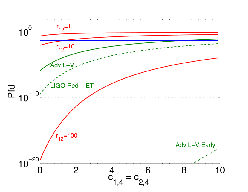
Figure 1: Comparative efficiency of the CC and alternative detection statistics. We take $T=10^{5}$ and $pfa=5\%$ and we assume that the signal is Gaussian ($c_{3}=c_{4}=0$) and that the noise distributions are symmetric ($c_{1,3}=c_{2,3}=0$). Various red plots correspond to different values for the ratio $r_{12}\equiv\dfrac{\sigma_{1}^{2}}{\sigma_{2}^{2}}=1,10,100,1000$. The parameter $\alpha$ is chosen so that the signal to noise ratio $SNR=\sqrt{T}\dfrac{\alpha^{2}}{\sigma_{2}\sigma_{2}}=3.28$, a value that yields a $pfd=5\%$ for the CC statistic in the homogeneous case $r_{12}=1$. When $c_{1,4}=c_{2,4}=0$, $pfd_{alt}\simeq 0.2,2\times 10^{-10},3\times 10^{-20}$ for $r_{12}=1,10,100$. The green plots correspond to realistic values for the cross-correlation between Advanced LIGO and Advanced Virgo at their nominal sensitivities ($r_{12}=48$) and between Einstein Telescope and Advanced LIGO with the LIGO Red possible upgraded sensitivity ($r_{12}=30$). We also considered an average value of $r_{12}=400$ corresponding to the cross-correlation between Advanced LIGO and Advanced Virgo during the early phases of the development of the detectors. When $c_{1,4}=c_{2,4}=0$, $pfd_{alt}\simeq 1\times 10^{-6},4\times 10^{-10},3\times 10^{-20},2\times 10^{-153}$ for $r_{12}=$ 30, 48 and 400.

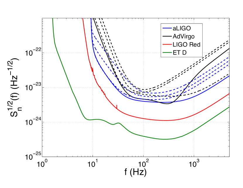
Figure 2: Expected sensitivity of Advanced LIGO and Advanced Virgo (blue and black continuous lines), LIGORed (dashed red line) and ET-D (green continuous line). The evolution of the sensitivity during the Advanced LIGO and Virgo early, middle and late phases are also shown in dashed blue and black lines.

In Fig. 3, we consider the dual perspective, where the probability of a false dismissal is plotted against the ratio $r_{12}$ for typical values of $c_{1,4}=c_{2,4}=0$, 3 and 10. Again, as the ratio increases, we find a small deterioration in the performance of the CC statistic (the probability of false dismissal increases from $pfd_{cc}\simeq 5\%$ for $r_{12}=1$ to $pfd_{cc}\simeq 8\%$ for $r_{12}=1000$) and a substantial improvement for the alternative statistic. In the case of a normally distributed noise process ($c_{1,4}=c_{2,4}=0$), the alternative statistic outperforms the CC statistic for values $r_{12}\geq 6$ and the probability of a false dismissal becomes negligible, as small as $pfd_{alt}\sim 4\times 10^{-10}$ for the pair Advanced LIGO and Advanced Virgo ($r_{12}\simeq 48$) and $pfd_{alt}\sim 1\times 10^{-6}$ for the pair LIGO Red and ET ($r_{12}\simeq 30$), which translates into a gain of 8 and 4 orders of magnitude, respectively, compared to the CC statistic. For the cross-correlation between Advanced LIGO and Advanced Virgo during the early stages of development ($r_{12}\simeq 400$), the probability of a false dismissal is almost zero ($pfd_{alt}\sim 2\times 10^{-153}$).

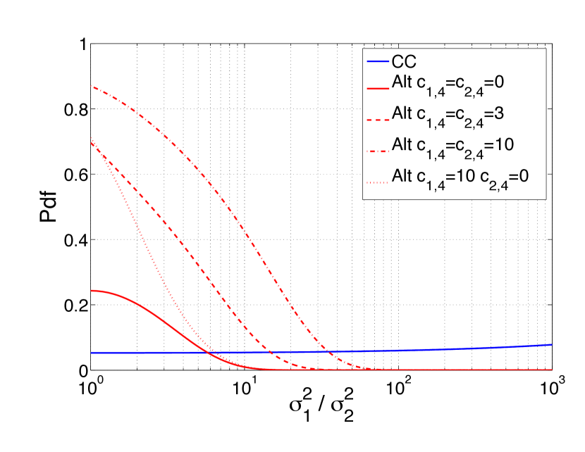
Figure 3: Probability of a false alarm for the CC and alternative detection statistics as a function of the ratio of detector sensitivities. We take $T=10^{5}$ and $pfa=5\%$ and we assume that the signal is Gaussian ($c_{3}=c_{4}=0$) and that the noise distributions are symmetric ($c_{1,3}=c_{2,3}=0$). Various red plots correspond to different choices for the pair of parameters $c_{1,4}$ and $c_{2,4}$. The parameter $\alpha$ is chosen so that the signal to noise ratio $SNR=\sqrt{T}\dfrac{\alpha^{2}}{\sigma_{2}\sigma_{2}}=3.28$, a value that yields a $pfd=5\%$ for the CC statistic in the homogeneous case $r_{12}\equiv\dfrac{\sigma_{1}^{2}}{\sigma_{2}^{2}}=1$.

So as to better understand why the presence of heterogenous detectors has such a strong impact on the relative efficiency of the CC versus alternative detection statistic, we consider two contrasted situations, a homogenous case situation (C1), with $\sigma_{1}=\sigma_{2}=\sigma$ and a heterogenous case situation (C2), with $\sigma_{1}=\dfrac{1}{\sigma}$ and $\sigma_{2}=\sigma^{3}$. We note that by construction the product $\sigma_{1}^{2}\sigma_{2}^{2}=\sigma^{4}$ in both cases but the sum $\sigma_{1}^{2}+\sigma_{2}^{2}$ is different and substantially higher in the heterogenous case situation.

Assuming Gaussian distributions for signal and noise, we have:

$$\mu_{CC}^{ns} = 0\text{, yielding the same value in C1 and C2}$$

$$\mu_{alt}^{ns} = \sigma_{1}^{2}\sigma_{2}^{2}\text{, yielding the same value in C1 and C2}$$

$$\sigma_{CC}^{2,ns} = \dfrac{\sigma_{1}^{2}\sigma_{2}^{2}}{T}\text{, yielding the same value in C1 and C2}$$

$$\sigma_{alt}^{2,ns} = \dfrac{8\sigma_{1}^{4}\sigma_{2}^{4}}{T}\text{, yielding the same value in C1 and C2}$$

and we also have:

$$\mu_{CC} = \alpha^{2}\text{, yielding the same value in C1 and C2}$$

$$\mu_{alt} = \sigma_{1}^{2}\sigma_{2}^{2}+\alpha^{2}\left(\sigma_{1}^{2}+\sigma_{2}^{2}\right)+3\alpha^{4}+c_{4}\text{, yielding a greater value for C2}$$

$$\sigma_{CC}^{2} = \dfrac{1}{T}\left(\sigma_{1}^{2}\sigma_{2}^{2}+\alpha^{2}\left(\sigma_{1}^{2}+\sigma_{2}^{2}\right)+2\alpha^{4}+c_{4}\right)\text{, yielding a greater value for C2}$$

$$\sigma_{alt}^{2} =$$ expression given in Eq. 24, yielding a greater value for C2

As a result, we find that the probability of a false alarm is the same in C1 and C2 for both the standard CC and the alternative detection statistics, since this probability only depends on the distributions of the detection statistics in the absence of a signal, which are the same for C1 and C2. In the presence of a signal, we find for the alternative statistic that moving from the homogenous case (C1) to the heterogeneous case (C2) leads to an increase in the mean, which has a positive impact on sensitivity, and an increase in the variance, which has a negative impact on sensitivity. Overall, the net effect is positive, as can be seen from Fig. 2 and 3. For the cross-correlation statistic, the mean is not impacted but there is an increase in variance, which is detrimental to detection. Overall, we confirm that the case with heterogeneous sensitivities is more favorable for the alternative statistic than it is for the CC detection statistic.

We now turn to the analysis of the impact of the 3rd moment of the noise distribution, which has been assumed to be zero so far. In Fig. 4, we show the probability of a false dismissal for the CC statistic (in blue) and the alternative statistic (in red) as a function of the third-order cumulant of the distribution of the noise for the first detector. We take $T=10^{5}$ and $pfa=5\%$ and we assume that the signal is Gaussian ($c_{3}=c_{4}=0$). We consider the homogeneous case $r_{12}\equiv\dfrac{\sigma_{1}^{2}}{\sigma_{2}^{2}}=1$. As usual, the parameter $\alpha$ is chosen so that the signal-to-noise ratio $SNR=\sqrt{T}\dfrac{\alpha^{2}}{\sigma_{2}\sigma_{2}}=3.28$, a value that yields a $pfd=5\%$ for the CC statistic for $r_{12}=1$. Various red plots correspond to different values for $c_{2,3}$, with $c_{4,i}=0$ for $i=1,2$, except for the crossed red line, where it is equal to 1. We find that the alternative statistic may dominate the CC statistic when $c_{1,3}$ and $c_{2,3}$ are of opposite signs. Indeed, the 3rd higher-order cumulants of the noise distributions do not impact the mean and variance of the CC statistic, but have an impact on the variance of the alternative statistic. Unlike the 4th order cumulant that is always positive, the 3rd higher-order cumulants can principle take on any negative or positive value, and taking them of opposite signs leads to a reduction in the variance of the alternative detection statistic. Indeed, these parameters enter the expression for the variance of the alternative statistic in Eq. 23 through the term $+16\mu_{2}\mu_{1,3}\mu_{2,3}$, which is negative when noise distributions have skewness parameters of opposite signs, suggesting a diversification effect (note that $\mu_{3}=c_{3}$ for centered distributions). On the other hand, we note again that an increase in $c_{4,i}$ (crossed red line in Fig. 3) leads to a deterioration of the performance of the alternative statistic.

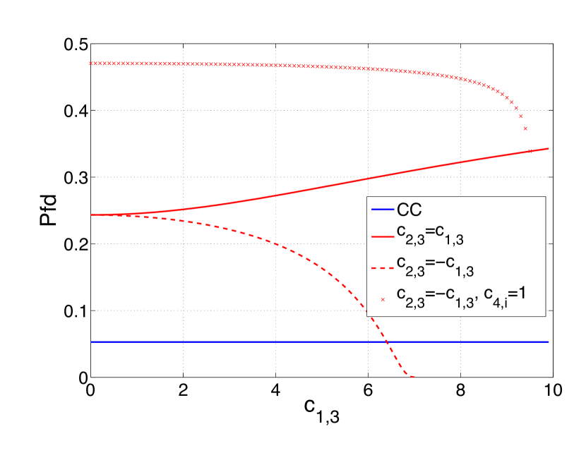
Figure 4: Impact of the skewness of the detector noise on the relative efficiency of the CC and alternative detection statistics for homogeneous detector sensitivities.. We take $T=10^{5}$ and $pfa=5\%$ and we assume that the signal is Gaussian ($c_{3}=c_{4}=0$). We consider the homogeneous case $r_{12}\equiv\dfrac{\sigma_{1}^{2}}{\sigma_{2}^{2}}=1$. The parameter $\alpha$ is chosen so that the signal to noise ratio $SNR=\sqrt{T}\dfrac{\alpha^{2}}{\sigma_{2}\sigma_{2}}=3.28$, a value that yields a $pfd=5\%$ for the CC statistic for $\dfrac{\sigma_{1}^{2}}{\sigma_{2}^{2}}=1$. Various red plots correspond to different choices of value for $c_{1,3}$ and $c_{2,3}$, with $c_{4,i}=0$ for $i=1,2$, except for the crossed red line, where it is equal to 1.

In Fig. 5, we repeat the analysis but focus on the case of heterogenous detector sensitivities by taking $r_{12}\equiv\dfrac{\sigma_{1}^{2}}{\sigma_{2}^{2}}=10$, while we had $r_{12}=1$ in Fig. 4.

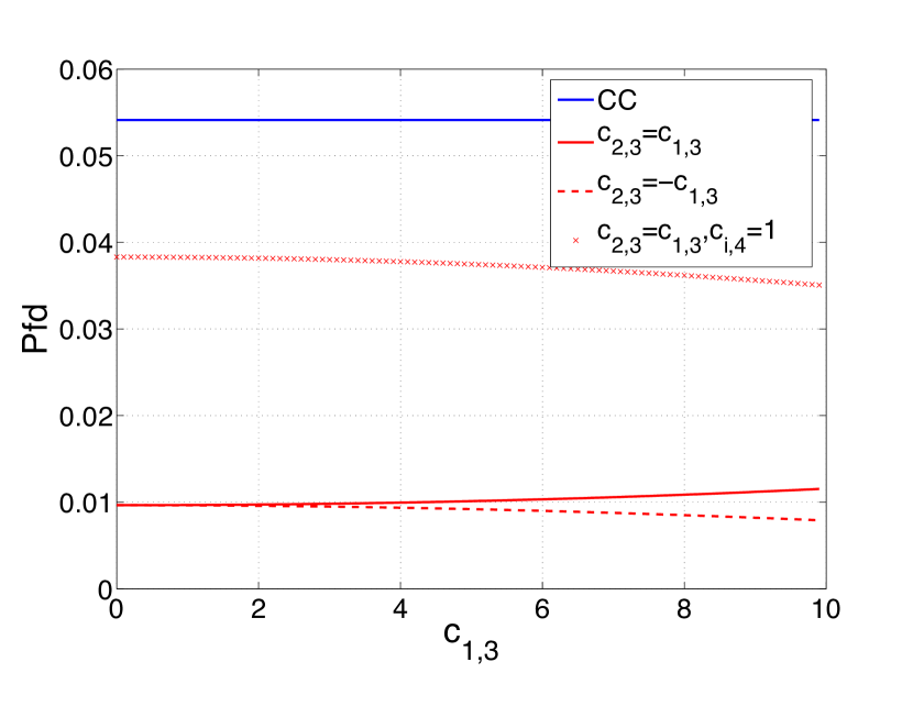
Figure 5: Impact of the skewness of the detector noise on the relative efficiency of the CC and alternative detection statistics for heterogeneous detector sensitivities. We take $T=10^{5}$ and $pfa=5\%$ and we assume that the signal is Gaussian ($c_{3}=c_{4}=0$). We consider the homogeneous case $r_{12}\equiv\dfrac{\sigma_{1}^{2}}{\sigma_{2}^{2}}=10$. The parameter $\alpha$ is chosen so that the signal to noise ratio $SNR=\sqrt{T}\dfrac{\alpha^{2}}{\sigma_{2}\sigma_{2}}=3.28$, a value that yields a $pfd=5\%$ for the CC statistic for $r_{12}=1$. Various red plots correspond to different choices of value for $c_{1,3}$ and $c_{2,3}$, with $c_{4,i}=0$ for $i=1,2$, except for the crossed red line, where it is equal to 1.

We find again that the alternative statistic dominates the CC statistic, an effect that is stronger when $c_{1,3}$ and $c_{2,3}$ are of opposite signs, but decreases when $c_{4,i}$ increases.

IV Estimation Methods for Non-Gaussian Signal and Non-Gaussian Noise Distributions

The analysis in the previous Section suggests that the use of the alternative statistic may lead to noticeable sensitivity gains when noise distributions are non-Gaussian and/or when detector sensitivities exhibit substantial differences. It should be noted, however, that using the alternative statistic requires in the non-Gaussian case the use of robust estimates not only for the variance, but also the skewness and kurtosis, of the signal and noise distributions. In what follows, we show how to obtain such estimates by extending standard maximum likelihood estimation methodologies to situations involving possibly non-Gaussian signal and noise distributions. As such, these results generalize early results reported by 2014PhRvD..89l4009M who have focussed on a situation involving a non-Gaussian signal distribution, while maintaining the assumption of a Gaussian noise distribution.

We denote by $f_{n_{i}}$ and $f_{s}$, respectively, the density function for the noise and the signal:

$$\Pr\left(\mathcal{N}_{i}\in\left[n,n+dn\right]\right) = f_{n_{i}}\left(n\right)dn$$

$$\Pr\left(\mathcal{S}\in\left[s,s+sn\right]\right) = f_{s}\left(s\right)ds$$

We also denote by $f_{n}\equiv f_{n}\left(n_{1t},n_{2t}\right)_{t=1,...,T}$ the joint probability distribution for the noise in the two detectors. The standard Bayesian approach for signal detection consists in finding the value for the unknown parameters so as to minimize the false dismissal probability at a fixed value of the false alarm probability. This criteria, known as the Neyman-Pearson criteria, is uniquely defined in terms of the so-called likelihood ratio $\Lambda$ given by:

$$\Lambda=\frac{\left.p_{h}\right|_{X=1}}{\left.p_{h}\right|_{X=0}}$$

where $\left.p_{h}\right|_{X=1}$ (respectively, $\left.p_{h}\right|_{X=0}$) is the conditional density for the measurement output if a signal is present (respectively, absent). A natural approximation of the likelihood ratio is the maximum likelihood detection statistic defined by 2003PhRvD..67h2003D :

$$\Lambda_{ML}=\frac{\underset{\alpha,\sigma_{1},\sigma_{2}}{\max}\int\left.f_{s}\right|_{X=1}\left(s\right)\left.f_{n}\right|_{X=1}\left(h-s\right)ds}{\underset{\sigma_{1},\sigma_{2}}{\max}\left.f_{n}\right|_{X=0}\left(h\right)}$$ (34)

and the maximum likelihood estimators for the unknown signal and noise standard-deviation parameters $\alpha,$ $\sigma_{1}$ and $\sigma_{2}$ are given as the corresponding likelihood maximizing quantities.

IV.1 Full Gaussian Case

It is typically assumed that both the noise and signal are normally distributed, $f_{n}$ and $f_{s}$ are Gaussian probability distribution functions, that is we may assume:

$$f_{n_{i}}\left(n_{it}\right) = \frac{1}{\sqrt{2\pi}\sigma_{i}}e^{-\frac{\left(n_{it}-\mu_{i}\right)^{2}}{2\sigma_{i}^{2}}}\text{ for }i=1,2$$

$$f_{s}\left(s_{t}\right) = \frac{1}{\sqrt{2\pi}\alpha}e^{-\frac{\left(s_{t}-\beta\right)^{2}}{2\alpha^{2}}}$$

where we also assume that both the noise and signal are weakly stationary processes so that their moments are constant through time. We further assume the noise in detector one and two are uncorrelated with a zero mean for both detectors. Under these assumptions, we have:

$$f_{n}\left(n_{1t},n_{2t}\right)=\frac{1}{2\pi\sigma_{1}\sigma_{2}}e^{-\frac{n_{1t}^{2}}{2\sigma_{1}^{2}}-\frac{n_{2t}^{2}}{2\sigma_{2}^{2}}}$$

and finally, assuming zero serial correlation:

$$f_{n} \equiv f_{n}\left(n_{1t},n_{2t}\right)_{t=1,...,T}=\prod\limits_{t=1}^{T}\frac{1}{2\pi\sigma_{1}\sigma_{2}}e^{-\frac{n_{1t}^{2}}{2\sigma_{1}^{2}}-\frac{n_{2t}^{2}}{2\sigma_{2}^{2}}}$$

$$f_{s} \equiv f_{s}\left(s_{t}\right)_{t=1,...,T}=\prod\limits_{t=1}^{T}\frac{1}{\sqrt{2\pi}\alpha}e^{-\frac{\left(s_{t}-\beta\right)^{2}}{2\alpha^{2}}}$$

Typically, one also assume that the mean value $\beta$ for the signal is zero so that the unknown parameters are $\alpha,$ $\sigma_{1}$ and $\sigma_{2}$. Then, we have that the denominator of equation (34) is given by:

$$\underset{\sigma_{1},\sigma_{2}}{\max}\left.f_{n}\right|_{X=0}\left(h\right)=\underset{\sigma_{1},\sigma_{2}}{\max}\prod\limits_{t=1}^{T}\frac{1}{2\pi\sigma_{1}\sigma_{2}}e^{-\frac{h_{1t}^{2}}{2\sigma_{1}^{2}}-\frac{h_{2t}^{2}}{2\sigma_{2}^{2}}}=\underset{\sigma_{1},\sigma_{2}}{\max}\frac{1}{\left(2\pi\sigma_{1}\sigma_{2}\right)^{T}}\exp\left[-\sum\limits_{t=1}^{T}\frac{h_{1t}^{2}}{2\sigma_{1}^{2}}-\sum\limits_{t=1}^{T}\frac{h_{2t}^{2}}{2\sigma_{2}^{2}}\right]$$

Introducing for $i=1,2$:

$$\overline{\sigma}_{i}^{2}=\frac{1}{T}\sum\limits_{t=1}^{T}h_{it}^{2}$$

we finally have that:

$$\underset{\sigma_{1},\sigma_{2}}{\max}f_{n}=\underset{\sigma_{1},\sigma_{2}}{\max}\frac{1}{\left(2\pi\sigma_{1}\sigma_{2}\right)^{T}}\exp\left[-\frac{T}{2}\left(\frac{\overline{\sigma}_{1}^{2}}{\sigma_{1}^{2}}+\frac{\overline{\sigma}_{2}^{2}}{\sigma_{2}^{2}}\right)\right]$$ (35)

It is straightforward to see that the maximum for equation (35) is reached for $\sigma_{i}^{2}=\overline{\sigma}_{i}^{2}$ and that maximum is given by:

$$\underset{\sigma_{1},\sigma_{2}}{\max}f_{n}=\frac{1}{\left(2\pi\overline{\sigma}_{1}\overline{\sigma}_{2}\right)^{T}}\exp\left[-\frac{T}{2}\left(1+1\right)\right]=\frac{1}{\left(2\pi\overline{\sigma}_{1}\overline{\sigma}_{2}\right)^{T}}\exp\left(-T\right)$$

Finally, we obtain the following expression:

$$\Lambda_{ML} = \frac{\underset{\alpha,\sigma_{1},\sigma_{2}}{\max}\int f_{s}\left(s\right)f_{n}\left(h-s\right)ds}{\underset{\sigma_{1},\sigma_{2}}{\max}f_{n}}$$

$$= \left(2\pi\overline{\sigma}_{1}\overline{\sigma}_{2}\right)^{T}\exp\left(T\right)\underset{\alpha,\sigma_{1},\sigma_{2}}{\max}\prod\limits_{t=1}^{T}\int_{-\infty}^{+\infty}f_{s}\left(s_{t}\right)\frac{1}{2\pi\sigma_{1}\sigma_{2}}\exp\left[-\frac{\left(h_{1t}-s_{t}\right)^{2}}{2\sigma_{1}^{2}}-\frac{\left(h_{2t}-s_{t}\right)^{2}}{2\sigma_{2}^{2}}\right]ds_{t}$$

$$= \underset{\alpha,\sigma_{1},\sigma_{2}}{\max}\prod\limits_{t=1}^{T}\frac{\overline{\sigma}_{1}\overline{\sigma}_{2}}{\sigma_{1}\sigma_{2}}\int_{-\infty}^{+\infty}f_{s}\left(s_{t}\right)\exp\left[-\frac{\left(h_{1t}-s_{t}\right)^{2}}{2\sigma_{1}^{2}}-\frac{\left(h_{2t}-s_{t}\right)^{2}}{2\sigma_{2}^{2}}+1\right]ds_{t}$$

We now specialize the analysis of the specific situation where the signal has a Gaussian distribution. In this case, and maintaining the assumption that the mean value for the signal is zero, we obtain:

$$f_{s}\equiv f_{s}\left(s_{t}\right)_{t=1,...,T}=\prod\limits_{t=1}^{T}\frac{1}{\sqrt{2\pi}\alpha}e^{-\frac{s_{t}^{2}}{2\alpha^{2}}}$$

We thus have:

$$\Lambda_{ML}=\underset{\alpha,\sigma_{1},\sigma_{2}}{\max}\prod\limits_{t=1}^{T}\frac{\overline{\sigma}_{1}\overline{\sigma}_{2}}{\sqrt{2\pi}\alpha\sigma_{1}\sigma_{2}}\int_{-\infty}^{+\infty}\exp\left[-\frac{s_{t}^{2}}{2\alpha^{2}}-\frac{\left(h_{1t}-s_{t}\right)^{2}}{2\sigma_{1}^{2}}-\frac{\left(h_{2t}-s_{t}\right)^{2}}{2\sigma_{2}^{2}}+1\right]ds_{t}$$

After tedious calculations, one obtains (see 2003PhRvD..67h2003D ):

$$\Lambda_{ML}=\underset{\alpha,\sigma_{1},\sigma_{2}\geq 0}{\max}\left\{\frac{\overline{\sigma}_{1}\overline{\sigma}_{2}}{\sqrt{\sigma_{1}^{2}\sigma_{2}^{2}+\sigma_{1}^{2}\alpha^{2}+\sigma_{2}^{2}\alpha^{2}}}\exp\left[\frac{\frac{\overline{\sigma}_{1}^{2}}{\sigma_{1}^{4}}+\frac{\overline{\sigma}_{2}^{2}}{\sigma_{2}^{4}}+\frac{2\overline{\alpha}^{2}}{\sigma_{1}^{2}\sigma_{2}^{2}}}{2\left(\frac{1}{\sigma_{1}^{2}}+\frac{1}{\sigma_{2}^{2}}+\frac{1}{\alpha^{2}}\right)}-\frac{\overline{\sigma}_{1}^{2}}{2\sigma_{1}^{2}}-\frac{\overline{\sigma}_{2}^{2}}{2\sigma_{2}^{2}}+1\right]\right\}^{T}$$ (36)

One can show that the maximum is reached for:

$$\alpha^{2} = \widehat{\alpha}^{2}\equiv\left(\overline{\alpha}^{2}\right)^{+}$$

$$\sigma_{i}^{2} = \widehat{\sigma}_{i}^{2}\equiv\left(\overline{\sigma}_{i}^{2}-\widehat{\alpha}^{2}\right)^{+}$$

where $\left(x\right)^{+}=x$ if $x>0$ and $\left(x\right)^{+}=0$ otherwise, which arise because of the positivity constraints on $\alpha,$ $\sigma_{1}$ and $\sigma_{2}$ in he maximization procedure.

The corresponding detection statistic is:

$$\Lambda_{ML}^{G}=\left(1-\frac{\widehat{\alpha}^{4}}{\overline{\sigma}_{1}^{2}\overline{\sigma}_{2}^{2}}\right)^{-T/2}$$ (37)

The cross-correlation statistic $\Lambda_{cc}^{G}$ can be obtained from $\Lambda_{ML}^{G}$ via a monotonic transformation which preserves false dismissal versus false alarm curves (see again 2003PhRvD..67h2003D ):

$$\Lambda_{cc}^{G}=\sqrt{1-\left(\Lambda_{ML}^{G}\right)^{-2/T}}=\frac{\widehat{\alpha}^{2}}{\overline{\sigma}_{1}\overline{\sigma}_{2}}$$ (38)

IV.2 Gaussian Signal and Non-Gaussian Noise

In 2014PhRvD..89l4009M , the Gaussian assumption was maintained for the detector noise distribution, but relaxed for the signal distribution. In what follows, we consider the opposite situation, namely a normally distributed signal, and a potentially non-Gaussian noise distribution. In other words, we assume:

$$f_{s}\left(s_{t}\right) = \frac{1}{\sqrt{2\pi}\alpha}e^{-\frac{s_{t}^{2}}{2\alpha^{2}}}\text{ }$$

$$f_{n_{i}}\left(n_{it}\right) \neq \frac{1}{\sqrt{2\pi}\sigma_{i}}e^{-\frac{n_{it}^{2}}{2\sigma_{i}^{2}}}\text{ for }i=1,2$$

As in 2014PhRvD..89l4009M , we propose to use a semi-parametric approach which allows one to approximate the unknown density as a transformation of a reference function (typically the Gaussian density), involving higher-order moments/cumulants of the unknown distribution. This approach has been heavily used in statistical problems involving a mild departure from the Gaussian distribution. In what follows, we will show that it allows us to obtain an analytical derivation of the nearly optimal maximum likelihood detection statistics for non-Gaussian gravitational wave stochastic backgrounds.

We want to approximate $f_{n_{i}}$, the density function of the unknown distribution of the noise distribution $\mathcal{N}_{i}$, as a function of the Gaussian density function $f_{n_{i}}^{G}\left(x\right)$ and a multiplicative deviation $g_{n_{i}}\left(x\right)$ from the Gaussian density function. To achieve this objective, we use the Edgeworth expansion, which is based on the assumption that the unknown signal distribution is the sum of normalized i.i.d. (non necessarily Gaussian) variables. In other words, it provides asymptotic correction terms to the Central Limit Theorem up to an order that depends on the number of moments available. When taken to the fourth-order level, the Edgeworth expansion reads as follows (see for example feller2008introduction (1971, P. 535) for the proof, and additional results regarding the convergence rate of the Edgeworth expansion):

$$f_{n_{i}}\left(x\right)\simeq f_{n_{i}}^{G}\left(x\right)\left[1+\frac{c_{i,3}}{6\sigma_{i}^{3}}H_{3}\left(\frac{x}{\sigma_{i}}\right)+\frac{c_{i,4}}{24\sigma_{i}^{4}}H_{4}\left(\frac{x}{\sigma_{i}}\right)+\frac{c_{i,3}^{2}}{72\sigma_{i}^{6}}H_{6}\left(\frac{x}{\sigma_{i}}\right)\right]$$ (39)

where the 6th Hermite polynomial is defined as $H_{6}\left(x\right)=x^{6}-15x^{4}+45x^{2}-15$. We finally have $f_{n_{i}}\left(x\right)\simeq f_{n_{i}}^{G}\left(x\right)g_{n_{i}}\left(x\right)$ with:

$$f_{n_{i}}^{G}\left(x\right) \equiv \frac{1}{\sqrt{2\pi}\sigma_{i}}\exp\left[-\frac{x^{2}}{2\sigma_{i}^{2}}\right]$$ (40)

$$g_{n_{i}}\left(x\right) \equiv \underset{b_{i,0}}{\underbrace{\left(1+\frac{c_{i,4}}{8\sigma_{i}^{4}}-\frac{5c_{i,3}^{2}}{24\sigma_{i}^{6}}\right)}}\underset{b_{i,1}}{\underbrace{-\frac{c_{i,3}}{2\sigma_{i}^{4}}}}x\underset{b_{i,2}}{+\underbrace{\left(\frac{15c_{i,3}^{2}}{24\sigma_{i}^{8}}-\frac{c_{i,4}}{4\sigma_{i}^{6}}\right)}}x^{2}+\underset{b_{i,3}}{\underbrace{\frac{c_{i,3}}{6\sigma_{i}^{6}}}}x^{3}+\underset{b_{i,4}}{\underbrace{\left(\frac{c_{i,4}}{24\sigma_{i}^{8}}-\frac{5c_{i,3}^{2}}{24\sigma_{i}^{10}}\right)}}x^{4}+\underset{b_{i,6}}{\underbrace{\frac{c_{i,3}^{2}}{72\sigma_{i}^{6}}}}x^{6}$$ (41)

In this context, the likelihood maximization problem becomes:

$$\Lambda_{ML} = \underset{\alpha,\sigma_{1},\sigma_{2},c_{1,3},c_{1,4},c_{2,3},c_{2,4}}{\max}\prod\limits_{t=1}^{T}\frac{\overline{\sigma}_{1}\overline{\sigma}_{2}}{\sqrt{2\pi}\alpha\sigma_{1}\sigma_{2}}\int_{-\infty}^{+\infty}\exp\left[-\frac{s_{t}^{2}}{2\alpha^{2}}-\frac{\left(h_{1t}-s_{t}\right)^{2}}{2\sigma_{1}^{2}}-\frac{\left(h_{2t}-s_{t}\right)^{2}}{2\sigma_{2}^{2}}+1\right]g_{n_{1}}\left(x\right)g_{n_{2}}\left(x\right)ds_{t}$$

$$= \underset{\alpha,\sigma_{1},\sigma_{2},c_{1,3},c_{1,4},c_{2,3},c_{2,4}}{\max}\prod\limits_{t=1}^{T}\frac{\sigma}{\alpha}\frac{\overline{\sigma}_{1}\overline{\sigma}_{2}}{\sigma_{1}\sigma_{2}}\exp\left[-\frac{h_{1t}^{2}}{2\sigma_{1}^{2}}-\frac{h_{2t}^{2}}{2\sigma_{2}^{2}}+1\right]\exp\left[\frac{1}{2}\sigma^{2}\left(\frac{h_{1t}}{\sigma_{1}^{2}}+\frac{h_{2t}}{\sigma_{2}^{2}}\right)^{2}\right]$$

$$\times\int_{-\infty}^{+\infty}\frac{1}{\sigma\sqrt{2\pi}}\exp\left[-\frac{1}{2\sigma^{2}}\left(s_{t}-\mu_{t}\right)^{2}\right]g_{n_{1}}\left(x\right)g_{n_{2}}\left(x\right)ds_{t}$$

with

$$\sigma = \left(\frac{1}{\alpha^{2}}+\frac{1}{\sigma_{1}^{2}}+\frac{1}{\sigma_{2}^{2}}\right)^{-\frac{1}{2}}$$

$$\mu_{t} = \left(\frac{h_{1t}}{\sigma_{1}^{2}}+\frac{h_{2t}}{\sigma_{2}^{2}}\right)\sigma^{2}$$

Focussing for simplicity of exposure on symmetric noise distribution functions (therefore such that $c_{i,3}=0$), we have:

$$g_{n_{1}}\left(x\right)g_{n_{2}}\left(x\right) = \left(b_{1,0}+b_{1,2}x^{2}+b_{1,4}x^{4}\right)\left(b_{2,0}+b_{2,2}x^{2}+b_{2,4}x^{4}\right)$$

$$= \beta_{0}+\beta_{2}x^{2}+\beta_{4}x^{4}+\beta_{6}x^{6}+\beta_{8}x^{8}$$

with:

$$\beta_{0} = b_{1,0}b_{2,0}$$

$$\beta_{2} = b_{1,0}b_{2,2}+b_{1,2}b_{2,0}$$

$$\beta_{4} = b_{1,0}b_{2,4}+b_{1,2}b_{2,2}+b_{2,0}b_{1,4}$$

$$\beta_{6} = b_{1,4}b_{2,2}+b_{1,2}b_{2,4}$$

$$\beta_{8} = b_{1,4}b_{2,4}$$

So we need to compute the following integrals, which can be obtained from the first moments of the Gaussian distribution:

$$I_{0} = \beta_{0}\int_{-\infty}^{+\infty}\frac{1}{\sigma\sqrt{2\pi}}\exp\left[-\frac{1}{2\sigma^{2}}\left(s_{t}-\mu_{t}\right)^{2}\right]ds_{t}=\beta_{0}$$

$$I_{2t} = \beta_{2}\int_{-\infty}^{+\infty}\frac{1}{\sigma\sqrt{2\pi}}s_{t}^{2}\exp\left[-\frac{1}{2\sigma^{2}}\left(s_{t}-\mu_{t}\right)^{2}\right]ds_{t}=\beta_{2}\left(\mu_{t}^{2}+\sigma^{2}\right)=\beta_{2}\left(\left(\frac{h_{1t}}{\sigma_{1}^{2}}+\frac{h_{2t}}{\sigma_{2}^{2}}\right)^{2}\sigma^{4}+\sigma^{2}\right)$$

$$I_{4t} = \beta_{4}\int_{-\infty}^{+\infty}\frac{1}{\sigma\sqrt{2\pi}}s_{t}^{4}\exp\left[-\frac{1}{2\sigma^{2}}\left(s_{t}-\mu\right)^{2}\right]ds_{t}=\beta_{4}\left(\mu_{t}^{4}+6\mu_{t}^{2}\sigma^{2}+3\sigma^{4}\right)$$

$$I_{6t} = \beta_{6}\int_{-\infty}^{+\infty}\frac{1}{\sigma\sqrt{2\pi}}s_{t}^{6}\exp\left[-\frac{1}{2\sigma^{2}}\left(s_{t}-\mu_{t}\right)^{2}\right]ds_{t}=\beta_{6}\left(\mu_{t}^{6}+15\mu_{t}^{4}\sigma^{2}+45\mu_{t}^{2}\sigma^{4}+15\sigma^{6}\right)$$

$$I_{8t} = \beta_{8}\int_{-\infty}^{+\infty}\frac{1}{\sigma\sqrt{2\pi}}s_{t}^{8}\exp\left[-\frac{1}{2\sigma^{2}}\left(s_{t}-\mu_{t}\right)^{2}\right]ds_{t}=\beta_{8}\left(\mu_{t}^{8}+28\mu_{t}^{6}\sigma^{2}+210\mu_{t}^{4}\sigma^{4}+420\mu_{t}^{2}\sigma^{6}+105\sigma^{8}\right)$$

Finally, we have that:

$$\Lambda_{ML} = \underset{\alpha,\sigma_{1},\sigma_{2},c_{1,4},c_{2,4}}{\max}\prod\limits_{t=1}^{T}\frac{\sigma}{\alpha}\frac{\overline{\sigma}_{1}\overline{\sigma}_{2}}{\sigma_{1}\sigma_{2}}\exp\left[-\frac{h_{1t}^{2}}{2\sigma_{1}^{2}}-\frac{h_{2t}^{2}}{2\sigma_{2}^{2}}+1\right]\exp\left[\frac{1}{2}\sigma^{2}\left(\frac{h_{1t}}{\sigma_{1}^{2}}+\frac{h_{2t}}{\sigma_{2}^{2}}\right)^{2}\right]$$ (43)

$$\times\left(I_{0}+I_{1t}+I_{2t}+I_{3t}+I_{4t}+I_{6t}+I_{8t}\right)$$

We note that when $c_{1,4}=c_{2,4}=0$, that is when the third and fourth-order cumulant vanish, as would be the case for a Gaussian distribution, then we have $I_{0}=1$, $I_{1}=I_{2}=I_{4}=I_{6}=I_{8t}=0,$ and we recover the maximum likelihood statistic of the Gaussian case:

$$\Lambda_{ML}^{G}=\underset{\alpha,\sigma_{1},\sigma_{2}}{\max}\prod\limits_{t=1}^{T}\frac{\sigma}{\alpha}\frac{\overline{\sigma}_{1}\overline{\sigma}_{2}}{\sigma_{1}\sigma_{2}}\exp\left[-\frac{h_{1t}^{2}}{2\sigma_{1}^{2}}-\frac{h_{2t}^{2}}{2\sigma_{2}^{2}}+1\right]\exp\left[\frac{1}{2}\sigma^{2}\left(\frac{h_{1t}}{\sigma_{1}^{2}}+\frac{h_{2t}}{\sigma_{2}^{2}}\right)^{2}\right]$$ (44)

In general, the presence of the additional terms implies a correction with respect to the Gaussian case. In the Gaussian case, one obtains the following explicit expressions for the variables involved in the maximization of the likelihood detection statistic 2003PhRvD..67h2003D :

$$\alpha^{2} = \widehat{\alpha}^{2}\equiv\left(\overline{\alpha}^{2}\right)^{+}$$

$$\sigma_{i}^{2} = \widehat{\sigma}_{i}^{2}\equiv\left(\overline{\sigma}_{i}^{2}-\widehat{\alpha}^{2}\right)^{+}$$

Here, the expression for the likelihood detection statistic is more involved and since it is not clear whether any analytical solutions can be obtained for the values for $\alpha,\sigma_{1},\sigma_{2},c_{1,4},c_{2,4}$ that would lead to the maximum in $\Lambda_{ML}$, one would need to resort to numerical optimization procedures. Taking the log, we have that:

$$\log\Lambda_{ML}=\underset{\alpha,\sigma_{1},\sigma_{2},c_{1,4},c_{2,4}}{\max}\log\Lambda_{ML}^{G}+\sum\limits_{t=1}^{T}\log\left(I_{0}+I_{1t}+I_{2t}+I_{3t}+I_{4t}+I_{6t}+I_{8t}\right)$$ (45)

IV.3 Non-Gaussian Signal and Noise Distributions

The methodology can also be extended to account for the presence of deviations from the Gaussian assumption for both the signal and noise distributions. To do so, we use again the Edgeworth expansion to approximate the unknown noise distribution as $f_{s}\left(x\right)\simeq f_{s}^{G}\left(x\right)g_{s}\left(x\right)$ and $f_{n_{i}}\left(x\right)\simeq f_{n_{i}}^{G}\left(x\right)g_{n_{i}}\left(x\right)$ with:

$$f_{s}^{G}\left(x\right) \equiv \frac{1}{\sqrt{2\pi}\alpha}\exp\left[-\frac{x^{2}}{2\alpha^{2}}\right]$$ (46)

$$g_{s}\left(x\right) \equiv \underset{b_{0}}{\underbrace{\left(1+\frac{c_{4}}{8\alpha^{4}}-\frac{5c_{3}^{2}}{24\alpha^{6}}\right)}}\underset{b_{1}}{\underbrace{-\frac{c_{3}}{2\alpha^{4}}}}x\underset{b_{2}}{+\underbrace{\left(\frac{15c_{3}^{2}}{24\alpha^{8}}-\frac{c_{4}}{4\alpha^{6}}\right)}}x^{2}+\underset{b_{3}}{\underbrace{\frac{c_{3}}{6\alpha^{6}}}}x^{3}+\underset{b_{4}}{\underbrace{\left(\frac{c_{4}}{24\alpha^{8}}-\frac{5c_{3}^{2}}{24\alpha^{10}}\right)}}x^{4}+\underset{b_{6}}{\underbrace{\frac{c_{3}^{2}}{72\alpha^{6}}}}x^{6}$$ (47)

$$f_{n_{i}}^{G}\left(x\right) \equiv \frac{1}{\sqrt{2\pi}\sigma_{i}}\exp\left[-\frac{x^{2}}{2\sigma_{i}^{2}}\right]$$ (48)

$$g_{n_{i}}\left(x\right) \equiv \underset{b_{i,0}}{\underbrace{\left(1+\frac{c_{i,4}}{8\sigma_{i}^{4}}-\frac{5c_{i,3}^{2}}{24\sigma_{i}^{6}}\right)}}\underset{b_{i,1}}{\underbrace{-\frac{c_{i,3}}{2\sigma_{i}^{4}}}}x\underset{b_{i,2}}{+\underbrace{\left(\frac{15c_{i,3}^{2}}{24\sigma_{i}^{8}}-\frac{c_{i,4}}{4\sigma_{i}^{6}}\right)}}x^{2}+\underset{b_{i,3}}{\underbrace{\frac{c_{i,3}}{6\sigma_{i}^{6}}}}x^{3}+\underset{b_{i,4}}{\underbrace{\left(\frac{c_{i,4}}{24\sigma_{i}^{8}}-\frac{5c_{i,3}^{2}}{24\sigma_{i}^{10}}\right)}}x^{4}+\underset{b_{i,6}}{\underbrace{\frac{c_{i,3}^{2}}{72\sigma_{i}^{6}}}}x^{6}$$ (49)

In this context, the likelihood maximization problem becomes:

$$\Lambda_{ML} = \underset{\begin{array}[]{c}\alpha,\sigma_{1},\sigma_{2},c_{3},c_{4},\\ c_{1,3},c_{1,4},c_{2,3},c_{2,4}\end{array}}{\max}\prod\limits_{t=1}^{T}\frac{\overline{\sigma}_{1}\overline{\sigma}_{2}}{\sqrt{2\pi}\alpha\sigma_{1}\sigma_{2}}\int_{-\infty}^{+\infty}\exp\left[-\frac{s_{t}^{2}}{2\alpha^{2}}-\frac{\left(h_{1t}-s_{t}\right)^{2}}{2\sigma_{1}^{2}}-\frac{\left(h_{2t}-s_{t}\right)^{2}}{2\sigma_{2}^{2}}+1\right]g_{s}\left(x\right)g_{n_{1}}\left(x\right)g_{n_{2}}\left(x\right)ds_{t}$$

$$= \underset{\begin{array}[]{c}\alpha,\sigma_{1},\sigma_{2},c_{3},c_{4},\\ c_{1,3},c_{1,4},c_{2,3},c_{2,4}\end{array}}{\max}\prod\limits_{t=1}^{T}\frac{\sigma}{\alpha}\frac{\overline{\sigma}_{1}\overline{\sigma}_{2}}{\sigma_{1}\sigma_{2}}\exp\left[-\frac{h_{1t}^{2}}{2\sigma_{1}^{2}}-\frac{h_{2t}^{2}}{2\sigma_{2}^{2}}+1\right]\exp\left[\frac{1}{2}\sigma^{2}\left(\frac{h_{1t}}{\sigma_{1}^{2}}+\frac{h_{2t}}{\sigma_{2}^{2}}\right)^{2}\right]$$

$$\times\int_{-\infty}^{+\infty}\frac{1}{\sigma\sqrt{2\pi}}\exp\left[-\frac{1}{2\sigma^{2}}\left(s_{t}-\mu_{t}\right)^{2}\right]g_{s}\left(x\right)g_{n_{1}}\left(x\right)g_{n_{2}}\left(x\right)ds_{t}$$

with:

$$\sigma = \left(\frac{1}{\alpha^{2}}+\frac{1}{\sigma_{1}^{2}}+\frac{1}{\sigma_{2}^{2}}\right)^{-\frac{1}{2}}$$

$$\mu_{t} = \left(\frac{h_{1t}}{\sigma_{1}^{2}}+\frac{h_{2t}}{\sigma_{2}^{2}}\right)\sigma^{2}$$

Focussing for simplicity of exposure on symmetric noise distribution functions, for which we have $c_{3},c_{1,3},c_{2,3}=0$, we obtain:

$$g_{s}\left(x\right)g_{n_{1}}\left(x\right)g_{n_{2}}\left(x\right) = \left(b_{0}+b_{2}x^{2}+b_{4}x^{4}\right)\left(b_{1,0}+b_{1,2}x^{2}+b_{1,4}x^{4}\right)\left(b_{2,0}+b_{2,2}x^{2}+b_{2,4}x^{4}\right)$$

$$= \gamma_{0}+\gamma_{2}x^{2}+\gamma_{4}x^{4}+\gamma_{6}x^{6}+\gamma_{8}x^{8}+\gamma_{8}x^{10}+\gamma_{8}x^{12}$$

with straightforward expressions for the $\gamma_{i}$ terms as a function of the $b_{1,i}$, $b_{2,i}$ and $b_{i}$ coefficients.

So we need to compute the following integrals, which can be obtained from the first moments of the Gaussian distribution:

$$I_{0} = \gamma_{0}\int_{-\infty}^{+\infty}\frac{1}{\sigma\sqrt{2\pi}}\exp\left[-\frac{1}{2\sigma^{2}}\left(s_{t}-\mu_{t}\right)^{2}\right]ds_{t}$$

$$I_{2t} = \gamma_{2}\int_{-\infty}^{+\infty}\frac{1}{\sigma\sqrt{2\pi}}s_{t}^{2}\exp\left[-\frac{1}{2\sigma^{2}}\left(s_{t}-\mu_{t}\right)^{2}\right]ds_{t}$$

$$I_{4t} = \gamma_{4}\int_{-\infty}^{+\infty}\frac{1}{\sigma\sqrt{2\pi}}s_{t}^{4}\exp\left[-\frac{1}{2\sigma^{2}}\left(s_{t}-\mu\right)^{2}\right]ds_{t}$$

$$I_{6t} = \gamma_{6}\int_{-\infty}^{+\infty}\frac{1}{\sigma\sqrt{2\pi}}s_{t}^{6}\exp\left[-\frac{1}{2\sigma^{2}}\left(s_{t}-\mu_{t}\right)^{2}\right]ds_{t}$$

$$I_{8t} = \gamma_{8}\int_{-\infty}^{+\infty}\frac{1}{\sigma\sqrt{2\pi}}s_{t}^{8}\exp\left[-\frac{1}{2\sigma^{2}}\left(s_{t}-\mu_{t}\right)^{2}\right]ds_{t}$$

$$I_{10t} = \gamma_{10}\int_{-\infty}^{+\infty}\frac{1}{\sigma\sqrt{2\pi}}s_{t}^{10}\exp\left[-\frac{1}{2\sigma^{2}}\left(s_{t}-\mu_{t}\right)^{2}\right]ds_{t}$$

$$I_{12t} = \gamma_{12}\int_{-\infty}^{+\infty}\frac{1}{\sigma\sqrt{2\pi}}s_{t}^{8}\exp\left[-\frac{1}{2\sigma^{2}}\left(s_{t}-\mu_{t}\right)^{2}\right]ds_{t}$$

Again, we need to compute higher-order moments of the Gaussian distribution, which is given by the following formula for a normally distributed variable $X$ with mean $\mu$ and variance:

$$\mathbb{E}\left(X^{n}\right)=\int_{-\infty}^{+\infty}\frac{1}{\sigma\sqrt{2\pi}}x^{n}\exp\left[-\frac{1}{2\sigma^{2}}\left(n-\mu\right)^{2}\right]dx=\sum\limits_{j=0}^{\left[\frac{n}{2}\right]}\binom{n}{2j}\left(2j-1\right)!!\sigma^{2j}\mu^{n-2j}$$ (52)

where $n!!$ denotes the double factorial operator $n!!=\prod\limits_{i=0}^{k}(n-2i)=n\left(n-2\right)\left(n-4\right)...$ with $k=\left[\frac{n}{2}\right]$.

For example, we have that:

$$I_{10t}=\gamma_{10}\left(\mu_{t}^{10}+45\mu_{t}^{8}\sigma^{2}+630\mu_{t}^{6}\sigma^{4}+3150\mu_{t}^{4}\sigma^{6}+4725\mu_{t}^{2}\sigma^{8}+945\sigma^{10}\right)$$ (53)

Finally, we have that:

$$\Lambda_{ML} = \underset{\begin{array}[]{c}\alpha,\sigma_{1},\sigma_{2},c_{3},c_{4},\\ c_{1,3},c_{1,4},c_{2,3},c_{2,4}\end{array}}{\max}\prod\limits_{t=1}^{T}\frac{\sigma}{\alpha}\frac{\overline{\sigma}_{1}\overline{\sigma}_{2}}{\sigma_{1}\sigma_{2}}\exp\left[-\frac{h_{1t}^{2}}{2\sigma_{1}^{2}}-\frac{h_{2t}^{2}}{2\sigma_{2}^{2}}+1\right]\exp\left[\frac{1}{2}\sigma^{2}\left(\frac{h_{1t}}{\sigma_{1}^{2}}+\frac{h_{2t}}{\sigma_{2}^{2}}\right)^{2}\right]$$ (57)

$$\times\left(I_{0}+I_{1t}+I_{2t}+I_{3t}+I_{4t}+I_{6t}+I_{8t}+I_{10t}+I_{12t}\right)$$

We note that when $c_{i,3}=c_{i,4}=0$, that is when the third and fourth-order cumulant vanish for the noise distribution, we then recover the maximum likelihood statistic from 2014PhRvD..89l4009M .

V Conclusions and Extensions

This paper analyzes the comparative efficiency of the standard CC detection statistic versus an alternative detection statistic obtained by cross-correlating squared measurements in situations involving non-Gaussian noise (and signal) distributions and heterogeneous detector sensitivities. We find that differences in detector sensitivities have a large impact on the efficiency of the CC detection statistic, which is dominated by the alternative statistic when these differences reach one order of magnitude. This effect is smaller in case of fat-tailed noise distributions, but it is magnified in case noise distributions have skewness parameters of opposite signs. On the other hand, higher-order cumulants of the signal distribution do not have a material impact on the relative efficiency of the two detection statistics in realistic situations where the signal is expected to be small compared to the noise. Since our methodology requires the estimation of higher-order moments/cumulants of the noise distribution, we extend the maximum likelihood estimator to the case of non-Gaussian signal and noise distributions and manage to recover analytical expressions for the log-likelihood function in case these distributions can be approximated by Edgeworth-type expansions.

Our methodology can be extended in a number of directions. We may first consider a setting involving a correlated noise component, typically regarded as environmental noise, in addition to the specific instrumental noise. On a different note, we have considered so far colocated and coincident detectors, an assumption which would hold in the case of Einstein Telescope. On the other hand, our framework should be extended to apply to a network of separated detectors such as Advanced LIGO-Virgo detectors, or joint observations by Advanced LIGO and Einstein Telescope. This extension is important because these are precisely the types of situations where differences in sensitivities are expected to be most substantial.

References

• [1] J. Aasi et al. Prospects for localization of gravitational wave transients by the advanced ligo and advanced virgo observatories. arXiv, 1304:0670, 2013.
• [2] B. Allen, J. D. E. Creighton, É. É. Flanagan, and J. D. Romano. Robust statistics for deterministic and stochastic gravitational waves in non-Gaussian noise: Frequentist analyses. Phys. Rev. D, 65(12):122002, June 2002.
• [3] B. Allen, J. D. E. Creighton, É. É. Flanagan, and J. D. Romano. Robust statistics for deterministic and stochastic gravitational waves in non-Gaussian noise. II. Bayesian analyses. Phys. Rev. D, 67(12):122002, June 2003.
• [4] B. Allen and J. D. Romano. Detecting a stochastic background of gravitational radiation: Signal processing strategies and sensitivities. Phys. Rev. D, 59(10):102001, May 1999.
• [5] A. Buonanno, M. Maggiore, and C. Ungarelli. Spectrum of relic gravitational waves in string cosmology. Phys. Rev. D, 55:3330–3336, March 1997.
• [6] A. Buonanno, G. Sigl, G. G. Raffelt, H.-T. Janka, and E. Müller. Stochastic gravitational-wave background from cosmological supernovae. Phys. Rev. D, 72(8):084001, October 2005.
• [7] C. Caprini, R. Durrer, T. Konstandin, and G. Servant. General properties of the gravitational wave spectrum from phase transitions. Phys. Rev. D, 79(8):083519, April 2009.
• [8] C. Caprini, R. Durrer, and G. Servant. Gravitational wave generation from bubble collisions in first-order phase transitions: An analytic approach. Phys. Rev. D, 77(12):124015, June 2008.
• [9] C. Caprini, R. Durrer, and G. Servant. The stochastic gravitational wave background from turbulence and magnetic fields generated by a first-order phase transition. Journal of Cosmology and Astroparticle Physics, 12:24, December 2009.
• [10] N. Christensen. Measuring the stochastic gravitational-radiation background with laser-interferometric antennas. Phys. Rev. D, 46:5250–5266, December 1992.
• [11] D. M. Coward and R. R. Burman. A cosmological ‘probability event horizon’ and its observational implications. Monthly Notices of the Royal Astronomical Society, 361:362–368, July 2005.
• [12] T. Damour and A. Vilenkin. Gravitational radiation from cosmic (super)strings: Bursts, stochastic background, and observational windows. Phys. Rev. D, 71(6):063510, March 2005.
• [13] J. C. N. de Araujo and G. F. Marranghello. Gravitational wave background from neutron star phase transition. General Relativity and Gravitation, 41:1389–1406, June 2009.
• [14] S. Drasco and É. É. Flanagan. Detection methods for non-Gaussian gravitational wave stochastic backgrounds. Phys. Rev. D, 67(8):082003, April 2003.
• [15] J.-F. Dufaux, D. G. Figueroa, and J. García-Bellido. Gravitational waves from Abelian gauge fields and cosmic strings at preheating. Phys. Rev. D, 82(8):083518, October 2010.
• [16] B. Barr et al. Ligo 3 strawman design, team red. 2012.
• [17] Willliam Feller. An introduction to probability theory and its applications. John Wiley & Sons, 2008.
• [18] V. Ferrari, S. Matarrese, and R. Schneider. Stochastic background of gravitational waves generated by a cosmological population of young, rapidly rotating neutron stars. Monthly Notices of the Royal astronomical Society, 303:258–264, February 1999.
• [19] E. E. Flanagan. Sensitivity of the Laser Interferometer Gravitational Wave Observatory to a stochastic background, and its dependence on the detector orientations. Phys. Rev. D, 48:2389–2407, September 1993.
• [20] M. Gasperini and G. Veneziano. Pre-big-bang in string cosmology. Astroparticle Physics, 1:317–339, July 1993.
• [21] L. P. Grishchuk. Amplification of gravitational waves in an isotropic universe. Soviet Journal of Experimental and Theoretical Physics, 40:409, September 1975.
• [22] L. P. Grishchuk. Relic gravitational waves and limits on inflation. Phys. Rev. D, 48:3513–3516, October 1993.
• [23] S. Hild, M. Abernathy, F. Acernese, P. Amaro-Seoane, N. Andersson, K. Arun, F. Barone, B. Barr, M. Barsuglia, M. Beker, N. Beveridge, S. Birindelli, S. Bose, L. Bosi, S. Braccini, C. Bradaschia, T. Bulik, E. Calloni, G. Cella, E. Chassande Mottin, S. Chelkowski, A. Chincarini, J. Clark, E. Coccia, C. Colacino, J. Colas, A. Cumming, L. Cunningham, E. Cuoco, S. Danilishin, K. Danzmann, R. De Salvo, T. Dent, R. De Rosa, L. Di Fiore, A. Di Virgilio, M. Doets, V. Fafone, P. Falferi, R. Flaminio, J. Franc, F. Frasconi, A. Freise, D. Friedrich, P. Fulda, J. Gair, G. Gemme, E. Genin, A. Gennai, A. Giazotto, K. Glampedakis, C. Gräf, M. Granata, H. Grote, G. Guidi, A. Gurkovsky, G. Hammond, M. Hannam, J. Harms, D. Heinert, M. Hendry, I. Heng, E. Hennes, J. Hough, S. Husa, S. Huttner, G. Jones, F. Khalili, K. Kokeyama, K. Kokkotas, B. Krishnan, T. G. F. Li, M. Lorenzini, H. Lück, E. Majorana, I. Mandel, V. Mandic, M. Mantovani, I. Martin, C. Michel, Y. Minenkov, N. Morgado, S. Mosca, B. Mours, H. Müller-Ebhardt, P. Murray, R. Nawrodt, J. Nelson, R. Oshaughnessy, C. D. Ott, C. Palomba, A. Paoli, G. Parguez, A. Pasqualetti, R. Passaquieti, D. Passuello, L. Pinard, W. Plastino, R. Poggiani, P. Popolizio, M. Prato, M. Punturo, P. Puppo, D. Rabeling, P. Rapagnani, J. Read, T. Regimbau, H. Rehbein, S. Reid, F. Ricci, F. Richard, A. Rocchi, S. Rowan, A. Rüdiger, L. Santamaría, B. Sassolas, B. Sathyaprakash, R. Schnabel, C. Schwarz, P. Seidel, A. Sintes, K. Somiya, F. Speirits, K. Strain, S. Strigin, P. Sutton, S. Tarabrin, A. Thüring, J. van den Brand, M. van Veggel, C. van den Broeck, A. Vecchio, J. Veitch, F. Vetrano, A. Vicere, S. Vyatchanin, B. Willke, G. Woan, and K. Yamamoto. Sensitivity studies for third-generation gravitational wave observatories. Classical and Quantum Gravity, 28(9):094013, May 2011.
• [24] E. Howell, D. Coward, R. Burman, D. Blair, and J. Gilmore. The gravitational wave background from neutron star birth throughout the cosmos. Monthly Notices of the Royal astronomical Society, 351:1237–1246, July 2004.
• [25] E. Howell, T. Regimbau, A. Corsi, D. Coward, and R. Burman. Gravitational wave background from sub-luminous GRBs: prospects for second- and third-generation detectors. Monthly Notices of the Royal astronomical Society, 410:2123–2136, February 2011.
• [26] G. Losurdo and the Advanced Virgo Team. Advanced virgo conceptual design. 2007.
• [27] S. Marassi, R. Ciolfi, R. Schneider, L. Stella, and V. Ferrari. Stochastic background of gravitational waves emitted by magnetars. Monthly Notices of the Royal astronomical Society, 411:2549–2557, March 2011.
• [28] S. Marassi, R. Schneider, G. Corvino, V. Ferrari, and S. P. Zwart. Imprint of the merger and ring-down on the gravitational wave background from black hole binaries coalescence. Phys. Rev. D, 84(12):124037, December 2011.
• [29] S. Marassi, R. Schneider, and V. Ferrari. Gravitational wave backgrounds and the cosmic transition from Population III to Population II stars. Monthly Notices of the Royal astronomical Society, 398:293–302, September 2009.
• [30] L. Martellini and T. Regimbau. Semiparametric approach to the detection of non-Gaussian gravitational wave stochastic backgrounds. Phys. Rev. D, 89(12):124009, June 2014.
• [31] D. Meacher, M. Coughlin, S. Morris, T. Regimbau, N. Christensen, S. Kandhasamy, V. Mandic, J. D. Romano, and E. Thrane. A Mock Data and Science Challenge for Detecting an Astrophysical Stochastic Gravitational-Wave Background with Advanced LIGO and Advanced Virgo. ArXiv e-prints, June 2015.
• [32] S. Ölmez, V. Mandic, and X. Siemens. Gravitational-wave stochastic background from kinks and cusps on cosmic strings. Phys. Rev. D, 81(10):104028, May 2010.
• [33] M Punturo et al. The einstein telescope: a third-generation gravitational wave observatory. Classical and Quantum Gravity, 27(19):194002, 2010.
• [34] T. Regimbau and J. A. de Freitas Pacheco. Cosmic background of gravitational waves from rotating neutron stars. Astronomy and Astrophysics, 376:381–385, September 2001.
• [35] T. Regimbau and J. A. de Freitas Pacheco. Gravitational wave background from magnetars. Astronomy and Astrophysics, 447:1–7, February 2006.
• [36] T. Regimbau, S. Giampanis, X. Siemens, and V. Mandic. Stochastic background from cosmic (super)strings: Popcorn-like and (Gaussian) continuous regimes. Phys. Rev. D, 85(6):066001, March 2012.
• [37] P. A. Rosado. Gravitational wave background from binary systems. Phys. Rev. D, 84(8):084004, October 2011.
• [38] P. A. Rosado. Gravitational wave background from rotating neutron stars. Phys. Rev. D, 86(10):104007, November 2012.
• [39] P. Sandick, K. A. Olive, F. Daigne, and E. Vangioni. Gravitational waves from the first stars. Phys. Rev. D, 73(10):104024, May 2006.
• [40] N. Seto. Non-Gaussianity analysis of a gravitational wave background made by short-duration burst signals. Phys. Rev. D, 80(4):043003, August 2009.
• [41] X. Siemens, V. Mandic, and J. Creighton. Gravitational-Wave Stochastic Background from Cosmic Strings. Physical Review Letters, 98(11):111101, March 2007.
• [42] A. A. Starobinskiǐ. Spectrum of relict gravitational radiation and the early state of the universe. Soviet Journal of Experimental and Theoretical Physics Letters, 30:682, December 1979.
• [43] the Advanced LIGO Team. Advanced LIGO reference design. 2007.
• [44] E. Thrane. Measuring the non-Gaussian stochastic gravitational-wave background: A method for realistic interferometer data. Phys. Rev. D, 87(4):043009, February 2013.
• [45] C. Wu, V. Mandic, and T. Regimbau. Accessibility of the gravitational-wave background due to binary coalescences to second and third generation gravitational-wave detectors. Phys. Rev. D, 85(10):104024, May 2012.
• [46] C.-J. Wu, V. Mandic, and T. Regimbau. Accessibility of the stochastic gravitational wave background from magnetars to the interferometric gravitational wave detectors. Phys. Rev. D, 87(4):042002, February 2013.
• [47] X.-J. Zhu, X.-L. Fan, and Z.-H. Zhu. Stochastic Gravitational Wave Background from Neutron Star r-mode Instability Revisited. Astrophys. J. , 729:59, March 2011.
• [48] X.-J. Zhu, E. Howell, and D. Blair. Observational upper limits on the gravitational wave production of core collapse supernovae. Monthly Notices of the Royal astronomical Society, 409:L132–L136, November 2010.
• [49] X.-J. Zhu, E. Howell, T. Regimbau, D. Blair, and Z.-H. Zhu. Stochastic Gravitational Wave Background from Coalescing Binary Black Holes. Astrophys. J. , 739:86, October 2011.
• [50] X.-J. Zhu, E. J. Howell, D. G. Blair, and Z.-H. Zhu. On the gravitational wave background from compact binary coalescences in the band of ground-based interferometers. Monthly Notices of the Royal astronomical Society, 431:882–899, May 2013.