MAD-TH-15-06

Dynamics of ${\cal N}=4$ supersymmetric field theories in 2+1 dimensions and their gravity dual

William Cottrell, James Hanson, and Akikazu Hashimoto

Department of Physics, University of Wisconsin, Madison, WI 53706, USA

In this note we consider ${\cal N}=4$ SYM theories in 2+1 dimensions with gauge group $U(N)\times U(M)$ and $k$ hypermultiplets charged under the $U(N)$. When $k>2(N-M)$, the theory flows to a superconformal fixed point in the IR. Theories with $k<2(N-M)$, on the other hand, flows to strong coupling. We explore these theories from the perspective of gravity dual. We find that the gravity duals of theories with $k<(N-M)$ contain enhancons even in situations where repulson singularities are absent. We argue that supergravity description is unreliable in the region near these enhancon points. Instead, we show how to construct reliable sugra duals to particular points on the Coulomb branch where the enhancon is screened. We explore how these singularities reappear as one moves around in Coulomb branch and comment on possible field theory interpretation of this phenomenon. In analyzing gauge/gravity duality for these models, we encountered one unexpected surprise, that the condition for the supergravity solution to be reliable and supersymmetric is somewhat weaker than the expectation from field theory. We also discuss similar issues for theories with $k=0$.

1 Introduction

Supersymmetric field theories exhibit rich dynamical phenomena which are nonetheless susceptible to explicit analysis. The nature of the dynamics vary depending on the number of dimensions and the amount of supersymmetries. Naturally, the most studied class is field theories in 3+1 dimensions. The ${\cal N}=4$ theories are conformal. ${\cal N}=2$ theories have quantum corrected moduli space. ${\cal N}=1$ theories generically exhibit dynamically generated superpotentials that give rise to vacuum selection and symmetry breakings. Quite a bit is also known about supersymmetric field theories in 2+1 dimensions. Certain aspects of dynamics in 2+1 dimensions can be inferred by looking at the system as a theory in 3+1 dimensions compactified on a circle. The basic picture in the case with 8 supercharges was considered in [1]. More recently, the case with 4 supercharges was studied in [2, 3].

A phenomena that is unique to 2+1 dimensions is dynamical breaking of supersymmetry in Chern-Simons-Yang-Mills theories with ${\cal N}=1$ [4], ${\cal N}=2$, or ${\cal N}=3$ [5, 6] supersymmetries. The spontaneous breaking of supersymmetry for these models was argued based on computation of the Witten index and the $s$-rule applied to their brane construction. When spontaneous breaking of supersymmetry occurs in a weakly coupled theory, one can analyze the vacuum energy, condensate, and the presence of Goldstone fermions explicitly (although somewhat messily.) From dimensional considerations and counting of parameters, one expects the vacuum energy to scale, for $(N/k)\gg 1$ as

$${\cal E}=\#(N/k)^{\#}g_{YM}^{2}$$ (1.1)

where $g_{YM}^{2}$ in $2+1$ dimensions has the dimension of energy, and $\#$’s are dimensionless constants of order one that should be computable from first principles. Such analysis is not immediately possible for these models because they are strongly coupled. Attempts to analyze these features often involve modifying the theory in the ultra-violet and tuning the parameters so that DSB takes place in a weakly coupled regime, e.g. [7].

One possible approach to access these features in this model is to invoke gauge-gravity duality where one hopes to capture the relevant supersymetry breaking dynamics in terms of degrees of freedom that are weakly coupled in the gravity description. This program has met with limited success so far [8, 9], in that the dual supergravity background contains singularities making its effective dynamics beyond the scope of the supergravity description. Perhaps one can work harder at extracting meaningful effective dynamics along the lines of [10], but how precisely to do that for our purpose is not completely clear at the moment.

The goal of this article is to retreat to a simpler system where the field theory dynamics is under better control and to explore the singularities which arise in the gravity dual. Specifically, we consider a class of supersymmetric field theories in 2+1 dimensions with ${\cal N}=4$ supersymmetries. These models generically have a moduli space of vacua, with various branches, whose structure can be subject to quantum corrections. Some points in moduli space such as the point where two branches meet often plays a special role. Presumably, the full diversity of phenomena on the field theory side is reflected on the gravity side in the resolution of singularities. It is tempting to propose that mapping out such correspondences would eventually have profound impact on understanding black hole, cosmology, and other gravitational phenomena involving singularities.

2 ${\cal N}=4$ field theories in 2+1 dimensions and their supergravity dual

In this section, we will review the supergravity solution which will be the focus of our analysis. The background in question was constructed explicitly in [11] where much of the details and the conventions can be found. Here, we will summarize key features in order to make this paper self contained, but the readers are referred to [11] for a more thorough account.

2.1 Basic Setup

The class of theories we consider consists of (2+1)d ${\cal N}=4$ SYM with gauge group $U(N)\times U(M)$ and $k$ fundamental hypermultiplets charged under $U(N)$. They are represented by a circular quiver of the form illustrated in figure 1.a. Such a model can be constructed from the type IIB brane configuration illustrated in figure 1.b. The construction involves 2 NS5-branes and $k$ D5-branes, $N_{2}=N$ “integer” D3-branes winding all the way around the $S^{1}$ of period $L$, and $N_{4}=M-N$ “fractional” D3-branes suspended between the two NS5-branes separated by the distance $bL$. In the $\alpha^{\prime}\rightarrow 0$ zero slope limit, most of the string states decouple and we obtain a 3+1 dimensional defect theory on $R^{1,2}\times S^{1}$. In the limit that $L$ goes to zero, momentum modes along the $S^{1}$ decouples and we obtain a theory in 2+1 dimensions.

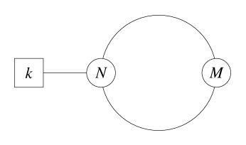
(a) (b)

Figure 1: Quiver diagram (a) and Hanany-Witten diagram (b) of $U(N)\times U(M)$ with $k$ flavors.

2.2 Supergravity solution

The gravity dual is most easily constructed by T-dualizing along $S^{1}$ which maps the 2 NS5-branes to $TN_{2}$ (which approaches the $C^{2}/Z_{2}$ ALE geometry in the $L\rightarrow 0$ limit), D5-branes to D6-branes, integer D3-branes to D2-branes, and fractional D3-branes to fractional D2-branes, which are D4-branes wrapping the collapsed 2-cycle at the tip of the $C^{2}/Z_{2}$ ALE.

One can then think of the IIA solution as a dimensional reduction of M-theory on $R^{1,2}\times(C^{2}/Z_{2})\times TN_{k}$ to which we add the back reaction of D2 and D4 branes sources. It is therefore natural to consider an ansatz where $R^{1,2}\times(C^{2}/Z_{2})\times TN_{k}$ gets warped as a result of fluxes sourced by the D2 and the D4-branes.

The ansatz considered in [11] is

$$ds^{2} = H^{-2/3}(-dt^{2}+dx_{1}^{2}+dx_{2}^{2})+H^{1/3}(ds_{ALE}^{2}+ds_{TN_{k}}^{2}),$$ (2.1)

$$G_{4} = dC_{3}=dt\wedge dx_{1}\wedge dx_{2}\wedge dH^{-1}+G_{4}^{SD},$$ (2.2)

$$G_{4}^{SD} = d(lV\omega_{2}\wedge\sigma_{3}+2\alpha\omega_{2}\wedge d\psi)$$ (2.3)

Let us make few comments regarding this ansatz.

• The Taub-NUT metric is given by

  $$ds_{TN_{k}}^{2}=V(r)^{-1}(dr^{2}+r^{2}(d\theta^{2}+\sin^{2}\theta d\phi^{2}))+V(r)R_{11}^{2}k^{2}\left(d\psi-{1\over 2}\cos\theta d\phi\right)^{2}$$ (2.4)

  with

  $$V(r)\equiv\left(1+{kR_{11}\over 2r}\right)^{-1},\qquad R_{11}=g_{s}l_{s}\ ,$$ (2.5)

  for the range of coordinates $0\leq r<\infty$, $0\leq\theta\leq\pi$, $0\leq\phi\leq 2\pi$, $0\leq\psi\leq 2\pi/k$. The parameter $k$ is related to the number of D6-branes

  $$k=N_{6}\ .$$ (2.6)

• 1-form $\sigma_{3}$ lives in the Taub-NUT space

  $${1\over 2}\sigma_{3}\equiv d\psi-{1\over 2}\cos\theta d\phi\ .$$ (2.7)

• The 2-form $\omega_{2}$ is dual to the collapsed 2-cycle of the $C^{2}/Z_{2}$ ALE. It is normalized so that

  $$\int_{ALE}\omega_{2}\wedge\omega_{2}={1\over 2}\ .$$ (2.8)

• The parameter $l$ parameterizes the magnitude of $G_{4}^{SD}$. The seemingly trivial parameter $\alpha$ which does not contribute to $G_{4}^{SD}$ on the account of $\omega_{2}$ and $d\psi$ being closed, will turn out to be important for quantizing charges.

• To solve the M-theory equation of motion, the warp factor $H$ must satisfy the Poisson equation

  $$0=\left(\nabla^{2}_{y}+\nabla^{2}_{TN}\right)H+{l^{2}V^{4}\over 2r^{4}}\delta^{4}(\vec{y})+(2\pi l_{p})^{6}Q_{2}\delta^{4}(\vec{y})\delta^{4}(\vec{r})\ ,$$ (2.9)

  where $\vec{y}$ is a four vector parameterizing $C^{2}/Z^{2}$, and $\vec{r}$ is a four vector parameterizing the Taub-NUT space. We have introduced another parameter $Q_{2}$ which corresponds to the magnitude of the D2-brane source which we will describe in more detail below.

• When expressed in terms of IIA supergravity fields, the solution takes the form

  $$ds_{IIA}^{2} = H^{-1/2}V^{1/2}(-dt^{2}+dx_{1}^{2}+dx_{2}^{2})+H^{1/2}V^{1/2}ds_{ALE}^{2}$$ (2.11)

  $$\qquad+H^{1/2}V^{-1/2}(dr^{2}+r^{2}(d\theta^{2}+\sin^{2}\theta d\phi^{2})),$$

  $$A_{1} = -{1\over 2}R_{11}k\cos\theta d\phi,$$ (2.12)

  $$A_{3} = -(H^{-1}-1)dt\wedge dx_{1}\wedge dx_{2}-lV\omega_{2}\wedge\cos\theta d\phi,$$ (2.13)

  $$B_{2} = -{2\over R_{11}k}(lV\omega_{2}+\alpha\omega_{2}),$$ (2.14)

  $$e^{\phi} = g_{s}H^{1/4}V^{3/4}.$$ (2.15)

  It is convenient to introduce a field variable $b$ by the relation

  $$B_{2}=(2\pi)^{2}\alpha^{\prime}b\,\omega_{2},$$ (2.16)

  so that

  $$b(r)=-{2\over(2\pi l_{s})^{2}R_{11}k}(lV+\alpha)$$ (2.17)

  is dimensionless.

• Parameters $\alpha$ and $l$ are fixed by imposing quantization of the D4-brane charge and the asymptotic behavior of $b(r)$ at $r=\infty$.

  Requiring that the D4 Page charge is integrally quantized leads to the relation

  $$2\pi\alpha=(2\pi l_{s})^{3}g_{s}N_{4}\ .$$ (2.18)

  One can then read off how $l$ depends on $b_{\infty}$ and $N_{4}$

  $$l=-2\pi^{2}kl_{s}^{2}Rb_{\infty}-\alpha=-(2\pi)^{2}g_{YM}^{2}\alpha^{\prime 2}\left(N_{4}+{kb_{\infty}\over 2}\right)\ .$$ (2.19)

  With supergravity parameters $l$ and $\alpha$ specified in terms of field theory data $b_{\infty}$ and $N_{4}$, we can write $b(r)$ more compactly as

  $$b(r)=b_{\infty}V(r)-{2N_{4}\over k}(1-V(r))$$ (2.20)

  so that $b(0)=(-2N_{4}/k)$ and $b(\infty)=b_{\infty}$.

  Note that something slightly unexpected has happened. The magnitude of gauge invariant field strength $G_{4}$ parameterized by $l$ depends on $b_{\infty}$ and is continuous, whereas seemingly gauge dependent parameter $\alpha$ depends on $N_{4}$ and is discrete.

• The last remaining parameter of the supergravity solution that needs to be related to the field theory data is $Q_{2}$ in (2.9). This parameter should be set so that the D2-page charge is integrally quantized, leading to the relation

  $$Q_{2}=N_{2}+b_{0}N_{4}+{N_{6}b_{0}^{2}\over 4}=N_{2}-{N_{4}^{2}\over k}$$ (2.21)

• To summarize, parameters $\alpha$, $l$, $k$, and $Q_{2}$ which appear as part of the supergravity ansatz is related to $N_{2}$, $N_{4}$, $N_{6}$, and $b_{\infty}$ by relations (2.6), (2.18), (2.19), and (2.21). $N_{2}$, $N_{4}$, $N_{6}$, and $b_{\infty}$ have natural interpretations on the field theory side. $N_{2}$, $N_{4}$, and $N_{6}$ take on integer values, whereas $b_{\infty}$ takes on continuous values in the range $0\leq b_{\infty}\leq 1$.

• With $Q_{2}$, $l$, and $\alpha$ parameterized in terms of $N_{2}$, $N_{4}$, and $b_{\infty}$, the Maxwell D2 and D4 charges becomes

  $$Q_{4}^{Maxwell} = N_{4}+{1\over 2}b_{\infty}N_{6},$$ (2.22)

  $$Q_{2}^{Maxwell} = N_{2}+b_{\infty}N_{4}+{1\over 4}b_{\infty}^{2}N_{6}.$$ (2.23)

• In order to identify the gravity solution we constructed with the brane configuration having the linking numbers illustrated in figure 1.b and not as illustrated in figure 2, we examine the probe action of D4-branes in this background.

  

  Figure 2: A brane configuration with flavors charged under both gauge groups.

  Consider a D4 or an anti D4 probe wrapping the collapsed 2-sphere at the tip of the ALE dual to $\omega_{2}$ threaded with $n$ units of magnetic flux. Provided

  $$(lV+\alpha)\pm 2\pi^{2}l_{s}^{2}R_{11}kn<0\ ,$$ (2.24)

  where $\pm$ corresponds to the D4 and the anti D4 respectively, the potential term in the DBI and the WZ terms cancel, giving rise to leading term in the derivative expansion of the form

  $$S = T_{4}\left(\left(2\pi^{2}l_{s}^{2}n\pm{\alpha\over kR_{11}}\right)V^{-1}\pm{l\over kR_{11}}\right)(\dot{r}^{2}+r^{2}\dot{\theta}^{2}+r^{2}\sin^{2}\theta\dot{\phi}^{2})$$ (2.25)

  $$\equiv {2\pi^{2}l_{s}^{2}T_{4}\over g_{eff}^{2}(r)}(\dot{r}^{2}+r^{2}\dot{\theta}^{2}+r^{2}\sin^{2}\theta\dot{\phi}^{2}),$$ (2.26)

  where

  $${1\over g_{eff}^{2}(r)}=(n\pm b_{\infty})+{R_{11}(nk\mp 2N_{4})\over 2r}\ .$$ (2.27)

  Performing the standard map between gauge theory and dual string theory parameters,

  $$R_{11}=g_{s}l_{s},\qquad r=2\pi l_{s}^{2}\Phi,\qquad g_{s}=g_{YM}^{2}(2\pi)^{-(p-2)}l_{s}^{-(p-3)},$$ (2.28)

  where $\Phi$ is the vacuum expectation value of the scalar field in along the Coulomb branch of the ${\cal N}=4$ gauge theory, we find

  $${1\over g_{eff}^{2}(\Phi)}=(n\pm b_{\infty})+{g_{YM}^{2}(nk\mp 2N_{4})\over 4\pi\Phi}\ .$$ (2.29)

  If one takes, $n=0$ for the “+” (D4-brane) and $n=1$ for the “$-$” (anti-D4-brane), the effective gauge couplings take the form

  $${1\over g_{eff1}^{2}(\Phi)} = b_{\infty}-{g_{YM}^{2}N_{4}\over 2\pi\Phi}\ ,$$ (2.30)

  $${1\over g_{eff2}^{2}(\Phi)} = (1-b_{\infty})+{g_{YM}^{2}(k+2N_{4})\over 4\pi\Phi}\ .$$ (2.31)

  This is interpretable as the expected running of the dimensionless coupling of the $U(N_{2}+N_{4})$ and the $U(N_{2})$ gauge groups, with $k$ fundamentals charged under $U(N_{2})$.

  The dimensionful gauge coupling for $U(N_{2}+N_{4})$ and $U(N_{2})$ in 2+1 dimensions at scale $\Phi$ is given,respectively by multiplying $g_{eff1}(\Phi)$ and $g_{eff2}(\Phi)$ by $g_{YM2})$. At the UV fixed point, they are, respectively, $g_{YM}^{2}b_{\infty}$ and $g_{YM}^{2}(1-b_{\infty})$.

• We know from field theory calculations that the perturbative moduli space of this theory is given by a multi-center Taub-Nut geometry described in (13) of [14]. This space is $4(N+M)$ real dimension hyper-Kahler geometry corresponding to $(N+M)$ D3 segments in Hanany-Witten brane construction, but we can infer a $4$ real dimensional subspace by keeping the position of the $(N+M-1)$ D3 segments fixed. This can be described, treating one of the $N$ D3-branes of the $U(N)\times U(M)$ theory as a probe, as the anti D4-brane probe with one unit of $D2$ charge. In order to infer the full hyper-Kahler structure, dualize the world-volume $(2+1)$ gauge field into a periodic scalar. In additon to the gauge field kinetic term, we must also account for the Wess-Zumino term:

  $$S\sim\left(B_{2}+2\pi\alpha^{\prime}f_{2}\right)\wedge C_{3}+...\\$$ (2.32)

  where $f_{2}$ is the field strength of the world volume gauge field. We have dropped terms which end up not contributing to integral over the two cycle wrapped by the probe. To construct the dual scalar form of the action, we add a lagrange multiplier to enforce the constraint $df_{2}=0$ and then treat $f_{2}$ as a free field. The relevant terms in the lagrangian are then:

  $$S_{\overline{D4}} \sim \int\left(\tilde{V}|f_{2}|^{2}-\frac{1}{4\pi}\left(d\varphi-(k+2N_{4})\cos\theta d\phi\right)\wedge f_{2}+...\right)$$ (2.33)

  where we have defined

  $$\tilde{V}\equiv g^{-2}_{eff2}\ .$$ (2.34)

  As usual, the dual scalar $\varphi$ is compact with periodicity $4\pi$. Now, integrate out $f_{2}$, and one gets

  $$S_{\overline{D4}}=\frac{1}{2(2\pi)^{2}g_{YM2}^{2}}\int dV_{3}\left((2\pi)^{2}\tilde{V}\left(\dot{\Phi}^{2}+\Phi^{2}\dot{\Omega}_{2}^{2}\right)+\frac{(g_{YM2}^{2})^{2}}{4\tilde{V}}\left(\dot{\varphi}-(k+2N_{4})\cos\theta\dot{\phi}\right)^{2}\right)$$ (2.35)

  Reading off the metric from the kinetic terms we find precisely the Taub-Nut-like metric expected from field theory. The fact that the moduli-space metric degenerates when $\tilde{V}$ becomes negative is a strong indication that the geometry must be corrected significantly inside the enhancon radius.

• It is natural to contemplate generalization with more than 2 NS5 branes and general linking numbers so that the flavors are charged more generally under the gauge group which has a product structure. Some preliminary discussion on this point is discussed in section 2.6.2 of [11]. See also [15]. Analyzing these constructions in detail appears somewhat subtle, and will be left for future work.

• It is also interesting to compare the IIA solution we reviewed here to the IIB solution discussed in [16, 17]. There are two main differences.

  One is that the solution of [16, 17] considers only the gravity dual of the IR fixed point, whereas we are considering the gravity dual of the full renormalization group flow starting with gauge field theory in the ultraviolet. We will study the intricacies of the renormalization group further in the following sections. These issues are inaccessible in the solutions of [16, 17].

  Another difference is the obvious one between the IIA and the IIB solutions. These are related by T-duality along the Hopf fiber direction of the ALE space. Usually, only one of the T-dual pair is the preferred duality frame in the sense that the effective dynamics is better encoded in the supergravity approximation. Whether one should or shouldn’t T-dualize along the Hopf fiber of the $C^{2}/Z_{k^{\prime}}$ orbifold has a lot to do with the size of $k^{\prime}$. When $k^{\prime}$ is large, it makes good sense to T-dualize from IIA to IIB [18]. In the case where $k^{\prime}=2$ as in the solution reviewed in this section, it is more effective to work in the IIA frame. The full string theory should, of course, encode all of the physics.

• The final step in constructing the solution is solving for the warp factor (2.9). Aside from the source term, (2.9) is linear. We can therefore break up $H(\vec{y},\vec{r})$ by writing

  $$H(\vec{y},\vec{r})=1+H_{1}(\vec{y},\vec{r})+H_{2}(\vec{y},\vec{r})$$ (2.36)

  where

  $$0 = \left(\nabla^{2}_{y}+\nabla^{2}_{TN}\right)H_{1}+(2\pi l_{p})^{6}Q_{2}\delta^{4}(\vec{y})\delta^{4}(\vec{r})$$ (2.37)

  $$0 = \left(\nabla^{2}_{y}+\nabla^{2}_{TN}\right)H_{2}+{l^{2}V^{4}\over 2r^{4}}\delta^{4}(\vec{y})$$ (2.38)

  with the boundary condition that $H^{1}$ and $H^{2}$ decay at infinity.

  $H_{1}(\vec{y},\vec{r})$ can be solved following [19], with the only difference being some factor of $2$ arising from the $Z_{2}$ orbifold in $C^{2}/Z_{2}$ and $k$ from the Taub-NUT charge. The solution is

  $$H_{1}(y,r) = (2k)32\pi^{2}l_{p}^{6}Q_{2}\int dp\left({(py)^{2}J_{1}(py)\over 4\pi^{2}y^{3}}\right)H_{1p}$$ (2.39)

  $$H_{1p} = c_{p}e^{-pr}{\cal U}\left(1+{kpR_{11}\over 4},2,2pr\right)$$ (2.40)

  $$c_{p} = \left({\pi^{2}\over 8}p^{2}\Gamma\left({pkR_{11}\over 4}\right)\right)$$ (2.41)

  Using similar separation of variable technique, we have for $H_{2p}$,

  $$H_{2}(r,y)=2\int dp\left({(py)^{2}J_{1}(py)\over 4\pi^{2}y^{3}}\right)H_{2p}$$ (2.42)

  with

  $$\left(\partial_{r}^{2}+{2\over r}\partial_{r}-{p^{2}\over V}\right)H_{2p}=-{l^{2}V^{3}\over 2r^{4}}$$ (2.43)

  which can formally be solved using the method of variation (See (1.5.7) of [20].)

  $$H_{2p}=H_{2p}^{(2)}(r)\int_{r_{1}}^{r}dr^{\prime}\left(-{l^{2}V^{3}\over 2r^{4}}\right){H_{2p}^{(1)}(r^{\prime})\over W(r^{\prime})}-H_{2p}^{(1)}(r)\int_{r_{2}}^{r}dr^{\prime}\left(-{l^{2}V^{3}\over 2r^{4}}\right){H_{2p}^{(2)}(r^{\prime})\over W(r^{\prime})}$$ (2.44)

  where

  $$W(r^{\prime})=H_{2p}^{(1)}(r^{\prime})H^{\prime}{}_{2p}^{(2)}(r^{\prime})-H_{2p}^{(2)}(r^{\prime})H^{\prime}{}_{2p}^{(1)}(r^{\prime})$$ (2.45)

  and

  $$H_{2p}^{(1)} = e^{-pr}{\cal U}\left(1+{pkR_{11}\over 4},2,2pr\right)$$ (2.46)

  $$H_{2p}^{(2)} = e^{-pr}{}_{1}F_{1}\left(1+{pkR_{11}\over 4},2,2pr\right)$$ (2.47)

  where $r_{1}$ and $r_{2}$ parameterizes the freedom to adjust the integration constant. In order to make the solution regular at $r=0$ and $r=\infty$, we set $r_{1}=\infty$ and $r_{2}=0$.

  The Wronskian for these solutions can be written compactly as

  $$W=H_{2p}^{(1)}(r)H_{2p}^{(2)}{}^{\prime}(r)-H_{2p}^{(2)}(r)H_{2p}^{(1)}{}^{\prime}(r)={2\over kp^{2}Rr^{2}\Gamma\left({1\over 4}kpR\right)}\ .$$ (2.48)

• We can now scale out $\alpha^{\prime}$ dependence by substituting

  $$r = \alpha^{\prime}U$$ (2.49)

  $$y = \alpha^{\prime}Y$$ (2.50)

  $$p = \alpha^{\prime-1}P$$ (2.51)

  as well as scaling

  $$H_{i}(y,u)=\alpha^{\prime-2}h_{i}(Y,U)\ .$$ (2.52)

  Then, we find

  $$h_{1}(Y,U) = (2k)32\pi^{2}g_{YM}^{4}Q_{2}\int dP\left({(PY)^{2}J_{1}(PY)\over 4\pi^{2}Y^{3}}\right)h_{1P}$$ (2.53)

  $$h_{1P} = C_{P}e^{-PU}{\cal U}\left(1+{kPg_{YM}^{2}\over 4},2,2PU\right)$$ (2.54)

  $$C_{P} = {\pi^{2}\over 8}P^{2}\Gamma\left({kPg_{YM}^{2}\over 4}\right)$$ (2.55)

  and

  $$h_{2}(U,Y)=2(2\pi)^{4}g_{YM}^{4}\left(N_{4}+{kb_{\infty}\over 2}\right)^{2}\int dP\left({(PY)^{2}J_{1}(PY)\over 4\pi^{2}Y^{3}}\right)h_{2p}$$ (2.56)

  $$h_{2p}=h_{2P}^{(2)}(U)\int_{\infty}^{U}dU^{\prime}\left(-{V^{3}\over 2U^{\prime 4}}\right){h_{2P}^{(1)}(U^{\prime})\over w(U^{\prime})}\ -h_{2P}^{(1)}(U)\int_{0}^{U}dU^{\prime}\left(-{V^{3}\over 2U^{\prime 4}}\right){h_{2P}^{(2)}(U^{\prime})\over w(U^{\prime})}$$ (2.57)

  where

  $$w(U^{\prime})=h_{2P}^{(1)}(U^{\prime})h^{\prime}{}_{2P}^{(2)}(U^{\prime})-h_{2P}^{(2)}(U^{\prime})h^{\prime}{}_{2P}^{(1)}(U^{\prime})={2\over g_{YM}^{2}kP^{2}U^{\prime 2}\Gamma({1\over 4}kPg_{YM}^{2})}$$ (2.58)

  and

  $$h_{2P}^{(1)} = e^{-PU}{\cal U}\left(1+{Pkg_{YM}^{2}\over 4},2,2PU\right)$$ (2.59)

  $$h_{2p}^{(2)} = e^{-PU}{}_{1}F_{1}\left(1+{Pkg_{YM}^{2}\over 4},2,2PU\right)$$ (2.60)

  The essential point to take away here is that the only place where $\alpha^{\prime}$ appears is in (2.52), and the decoupling $\alpha^{\prime}\rightarrow 0$ has the effect of simply dropping the “1” in (2.52) while keeping everything else in (2.54)–(2.60) fixed. This will result in having the string frame metric having no dependence on $\alpha^{\prime}$ aside from the overall normalization

  $$ds^{2}=\alpha^{\prime}(\ldots)$$ (2.61)

  as is conventional in gauge gravity correspondences.

• Large/small radius behavior of the warp factor

  Now that we have worked out the warp factor in a reasonably explicit form, we can explore their asymptotic behaviors. The large and small radius behavior of $h_{1}(Y,U)$ is identical to what was found in [19]. In particular, for large $U^{2}+Y^{2}$, we find

  $$h_{1}(Y,U)\sim{12\pi^{2}g_{YM}^{2}}{Q_{2}\over(U^{2}+Y^{2})^{5/2}}\ ,$$ (2.62)

  which is the warp factor expect for D2-brane in $C^{2}/Z_{2}\times R^{3}$.

  For $h_{2}(Y,U)$, we find

  $$h_{2}(Y,U)\sim 12\pi^{2}g_{YM}^{2}{{1\over k}\left(N_{4}+{kb_{\infty}\over 2}\right)^{2}\over(U^{2}+Y^{2})^{5/2}}\ .$$ (2.63)

  The numerator

  $$Q_{bulk}={1\over k}\left(N_{4}+{kb_{\infty}\over 2}\right)^{2}$$ (2.64)

  can be interpreted as the bulk contribution to Maxwell charge so that

  $$Q_{Maxwell}=Q_{2}+Q_{bulk}=N_{2}+b_{\infty}N_{4}+{1\over 4}b_{\infty}^{2}k$$ (2.65)

  For small $U$ and $Y$, on the other hand, we find that

  $$h_{1}(Y,U)={64\pi^{2}kg_{YM}^{4}\over(Y^{2}+2kg_{YM}^{2}U)^{3}}Q_{2},\qquad h_{2}(Y,U)={64\pi^{2}\over g_{YM}^{4}k^{4}}{\left(N_{4}+{bk\over 2}\right)^{2}\over Y^{2}}$$ (2.66)

  which takes on somewhat more homogeneous form when we substitute

  $$U={Z^{2}\over 2kg_{YM}^{2}}$$ (2.67)

  so that

  $$h_{1}(Y,Z)={64\pi^{2}kg_{YM}^{4}\over(Y^{2}+Z^{2})^{3}}Q_{2},\qquad h_{2}(Y,Z)={64\pi^{2}\over g_{YM}^{4}k^{4}}{\left(N_{4}+{bk\over 2}\right)^{2}\over Y^{2}}$$ (2.68)

  What we see is that $h_{2}$ sources a wall of charges localized at $Y=0$ which dominates when $Q_{2}=0$. If $Q_{2}$ is positive, however, $h_{1}$ dominates near $Y=Z=0$, and asympototes to an $AdS_{4}\times S_{7}/Z_{k}$ geometry whose radius in Plank unit is $Q_{2}$ up to some finite dimensionless factor. If on the other hand $Q_{2}$ is negative but $Q_{2}^{Maxwell}$ is positive, then the background will contain a repulson singularity which one expects to be resolved by the standard enhancon mechanism. What is interesting about this class of background, however, is the fact that the enhancon mechanism can be relevant even in the absence of repulson singularities, as we will discuss further below.

2.3 Holographic interpretation of the supergravity solution

Now that we have worked out the supergravity solution in detail, let us examine their basic properties. The D2 Maxwell charge was found to be

$$Q_{2}^{Maxwell}=N_{2}+b_{\infty}N_{4}+{b_{\infty}^{2}\over 4}k\ .$$ (2.69)

Let us restrict our attention to the case where this charge is positive.

The D2 brane charge localized at the origin, on the other hand, was found to be

$$Q_{2}=N_{2}-{N_{4}^{2}\over k}\ .$$ (2.70)

If $Q_{2}$ is positive, we find that the region near the origin asymptotes to $AdS_{4}\times S^{7}/Z_{k}$ with curvature of order $Q_{2}$, as was found in [11, 21]

If instead $Q_{2}$ takes a negative value while keeping $Q_{2}^{Maxwell}$ positive, we encounter a singularity of a repulson type. If all the objects giving rise to net negative $Q_{2}$ are allowed BPS objects e.g. flux and discrete torsion, this repulson singularity is expected to be resolved by the standard enhancon mechanism and ultimately give rise to regular string dynamics [22]. If $Q_{2}\ll-1$, the configuration like does not exist as a supersymmetric state.

Let us examine the solution more closely for explicit choice of parameters.

• As the first concrete example, let us set

  $$b_{\infty}={1\over 2},\qquad N_{2}=2m,\qquad N_{4}=-m,\qquad k=N_{6}=3m\ .$$ (2.71)

  We will take $m$ to be some large but finite integer, so that the supergravity solution is effective for a wide range of scales [23]. We then have

  $$Q_{2}={5\over 3}m>0,\qquad Q_{2}^{Maxwell}={27\over 16}m>0\ .$$ (2.72)

  What we propose to do now is to probe this geometry in the $\Phi\sim r$ coordinates using a D4 and an anti D4+D2 probes fixed at the origin in the $\vec{y}$ coordinates. This is a crude probe of the Coulomb branch of the corresponding field theory.

  

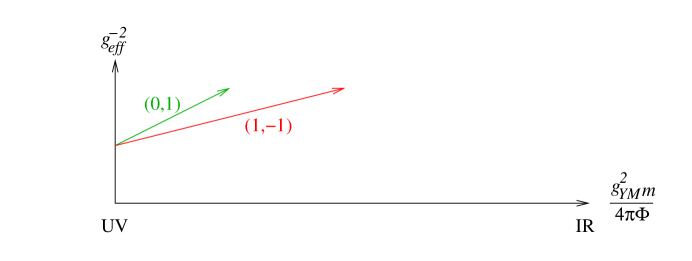
  Figure 3: $g_{eff}^{-2}$ for D4 or anti D4 probe with some D2 charge, as a function of $\Phi$. The notation (D2,D4) represents the charge of the probe. For instance $(0,1)$ is a D4 probe, and $(1,-1)$ is an anti D4 probe with one unit of D2 charge.

  If one plots $g_{eff1}^{-2}$ and $g_{eff2}^{-2}$ as given in (2.30) and (2.31), it would look like what is illustrated in figure 3. In particular, $g_{eff1}^{-2}$ and $g_{eff2}^{2}$ remains positive. This is equivalent to the condition that these probes satisfy (2.24) and remain BPS as they explore the entire range of $\Phi$.

  Nothing out of the ordinary happens, and the interpretation that this gravity solution is describing the RG flow of ${\cal N}=4$ $U(2m)\times U(m)$ system with $3m$ fundamentals in 2+1 dimensions, flowing in the IR to a superconformal fixed point dual to an $AdS_{4}\times S^{7}/Z_{3m}$ geometry of radius $5m/3$ appears rather robust.

• As a second example, consider setting

  $$b_{\infty}={1\over 2},\qquad N_{2}=2m,\qquad N_{4}=m,\qquad k=N_{6}=3m\ .$$ (2.73)

  The only change is the sign of $N_{4}$. It is easy to see that the this example is related to the previous one by the exchange of the position of the NS5-branes in the brane picture.

  For this example, we have

  $$Q_{2}={5\over 3}m>0,\qquad Q_{2}^{Maxwell}={43\over 16}m>0\ .$$ (2.74)

  So $Q_{2}$ is the same as in the previous example.

  The $g_{eff1,2}^{-2}$ look very different in this case. In particular, the effective coupling diverges as one flows from large to small $\Phi$ for the D4 probe at

  $${g_{YM}^{2}m\over 4\pi\Phi_{e}}={1\over 4}\ .$$ (2.75)

  This is illustrated in figure 4. For $\Phi<\Phi_{e}$, the D4 probe is no longer BPS.

  

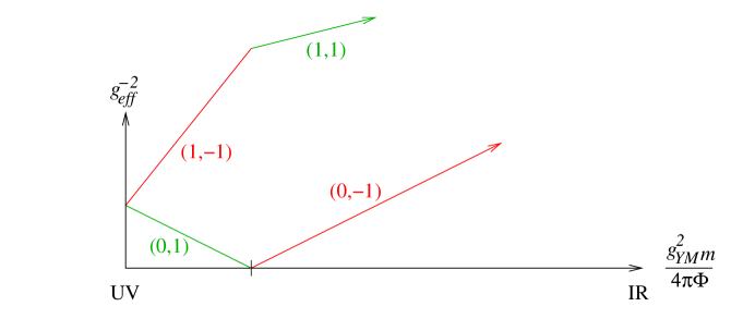
  Figure 4: $g_{eff}^{-2}$ for probe branes in the second case (or with $N_{4}$ positive). Inside the enhancon radius different probes are BPS.

  As it turns out, there are other probe which are BPS and can seemingly probe the region $\Phi<\Phi_{e}$. In the region $\Phi<\Phi_{e}$, one can use the $(1,1)$ and the $(0,-1)$ probes. These branes will probe the $AdS_{4}\times S^{7}/Z_{3m}$ geometry deep in the small $\Phi$ region without any problems.

• As the third example, let us consider the case

  $$b_{\infty}={1\over 2},\qquad N_{2}=7m,\qquad N_{4}=-4m,\qquad k=N_{6}=3m$$ (2.76)

  so that

  $$Q_{2}={5\over 3}m>0,\qquad Q_{2}^{Maxwell}={83\over 16}m>0\ .$$ (2.77)

  This time, we see the $(1,-1)$ probe cease to be BPS at

  $${g_{YM}^{2}m\over 4\pi\Phi_{e}}={1\over 10}\ .$$ (2.78)

  We can continue to probe the region $\Phi<\Phi_{e}$ using probes with charges $(-1,1)$ and $(2,-1)$. The $(2,-1)$ probe eventually ceases to be BPS, but one can probe beyond that region using yet another set of probes $(3,-1)$ and $(-2,1)$. This set of probes remain BPS and valid all the way down to the origin in $\Phi$ space where the geometry asymptotes to $AdS_{4}\times S_{7}/Z_{3m}$.

  

  Figure 5: $g_{eff}^{-2}$ for probe branes in the third case. There are two enhancon radii and in each region there are different BPS probes.

What we seemingly have at our hand is a gravity solution dual to $U(2m)\times U(m)$, $U(2m)\times U(3m)$, and $U(7m)\times U(3m)$ theories with 3 fundamentals charged under the $U(2m)$ or $U(7m)$, which are free of repulson singularities, and seemingly all asymptoting to an $AdS_{4}\times S^{7}/Z_{k}$ geometry in the IR with radius $5m/3$. It is tempting, as was suggested in [24] to regard these backgrounds as exhibiting an analogue of duality cascade [25]. This then amounts to claiming that the three gauge theories listed above are related by Seiberg-like duality, and all have the same superconformal field theory as the infra-red fixed point.

There is however a main flaw in this argument. Seiberg’s duality in 3+1 dimensions [26] and the related Aharony duality in 2+1 dimensions [27] are features of field theories with 4 supercharges. For theories with 8 supercharges like the ones we are considering, there is no established duality can be considered analogous. In the absence of dualities, one can not conceive of a duality cascade.

Another obvious difficulty in claiming that the three field theories considered as an example above are related by duality is the basic fact that the dimension and the structure of moduli space is completely incompatible.

This issue was articulated explicitly in [28] for ${\cal N}=2$ theories in 3+1 dimensions. In order to provide some holographic interpretation to the supergravity solution like the one we constructed in the last subsection, [28] suggested that the background is dual to some specific choice of vacuum on the Coulomb branch where the effective rank of the field theory is gradually reduced by Higgs mechanism.

This issue was further elaborated in [29] which constructed the supergravity solutions that are interpretable as being the dual of the ${\cal N}=2$ theory in 3+1 dimensions. By providing explicit supergravity solution for generic vacuum on the Coulomb branch, one can diagnose the hypothesis that the solutions found in the previous subsection is interpretable as some specific choice among the set of possible vacua. In this regard, the conclusion is somewhat anti-climactic. As long as the scale of the vacuum expectation value is greater than the scale set by $\Phi_{e}$, one can reliably interpret the supergravity solution, but as one approach near the origin/root of the Coulomb branch, the supergravity solution is suffering from being unreliable on the account of tensionless brane objects nucleating at the enhancon radius $\Phi_{e}$.

The crude diagnostic is that regions behind the first enhancon radius appearing at scale $\Phi_{e}$ do not exist unless the theory is sufficiently higgsed at scale exceeding $\Phi_{e}$. In the case of ${\cal N}=2$ theories in 3+1 dimensions, one can further argue that $\Phi_{e}$ is the minimal allowed higgsing that is allowed due to quantum corrections on the Coulomb branch which are analyzable using the technology of Seiberg-Witten theory [30, 31]. In particular, one can identify a special point on Coulomb branch called the “baryonic root” which is a unique point where the Coulomb branch and the baryonic branch meet [32]. For the supergravity duals of ${\cal N}=2$ theories in 3+1 dimensions, [29] showed that the dual of the baryonic root corresponds to arranging the fractional branes exactly at $\Phi_{e}$ to screen the enhancon.

Our ultimate goal to study these issues for the case of 2+1 dimensions. There are few obstacles that one needs to overcome in order to carry out this program in full. One is the fact that the technology of Seiberg-Witten theory is not as developed in 2+1 dimensions. We need to map out the structure intersections of Coulomb and Higgs branches for the ${\cal N}=4$ theories. There have been a number of useful recent developments e.g. [33, 34, 35] which we intend to exploit to develop this side of the story further.

In this article, we will take the first step in this program by constructing supergravity solutions which screens the enhancon singularity. More specifically, we construct the analogues of the explicitly higgsed solution of [29].

The essential conclusion we will arrive at is that gravity solution which exhibits an enhancon, even in the absence of a repulson, should be considered unreliable inside the enhancon radius. That certain seemingly good supergravity solution is nonetheless unreliable because of the behavior of probe branes may have far reaching impacts in subjects such as black hole information paradox, since vacua with fluxes and orbifold fixed points that give rise to these enhancon like structures is rather ubiquitous in string theory.

It is also useful to pause and note that the breakdown of supergravity due to enhancon mechanism does not always need to happen. In fact, it did not in the first example illustrated in figure 3. The condition for enhancons not to appear is for (2.30) and (2.31) to both exhibit the IR free running. In other words,

$$k\geq-2N_{4}\geq 0\ .$$ (2.79)

This is to be combined with the other requirement

$$Q_{2}=N_{2}-{N_{4}^{2}\over k}>0\ .$$ (2.80)

These are the conditions that the supergravity solution is well behaved.

Here, however, we encounter a curoius puzzle. In order for the brane configuration underlying the construction to preserve supersymmetry, we expect the condition

$$N_{2}>-N_{4}>0$$ (2.81)

to be satisfied. If (2.81) is violated, there will be some anti D3 segements as is illustrated in figure 6 which one expects will lead to the complete breaking of supersymmetry.

Figure 6: Hanany Witten type brane configuration for $N_{2}+N_{4}<0$.

The conditions (2.79) and (2.81) combined is equivalent to the criteria for the circular quiver to be of the “good” type (in the classification of [36]) as was specified by conditions

$$\rho^{T}>\rho$$ (2.82)

in (2.25) of [17] and $L\geq 0$. One can further show that given (2.79), condition (2.80) is strictly weaker than (2.81). This however creates an interesting conundrum. The supergravity solution satisfying (2.80) but violating (2.81) appears to be perfectly sensible supersymmetric background although we expect its field theory dual not to be supersymmetric. We will comment further on this puzzle in the Conclusions.

3 Higgsing

In this section, we construct a generalization of the supergravity solution constructed in the previous section where we higgs the $U(N)\times U(M)$ theory to $U(N)\times U(M-P)\times U(1)^{P}$ by moving $P$ fractional branes away from the origin in the $\vec{r}$ direction transverse to the D6-brane, which is taken to be positioned at the origin. Since these configurations are BPS, the $P$ fractional branes an be positioned arbitrarily in $\vec{r}$ space, but to keep the analysis simple, we will only consider the case where the $P$ branes are distributed uniformly along a spherical shell at some fixed radius $r_{s}$.

We will trace the construction of the unhiggsed solution by introducing the D6 brane first, followed by the D4 brane, followed by the D2 brane.

Let us therefore start with the $R^{1,2}\times(C^{2}/Z_{2})\times TN_{k}$ geometry in 11 dimensions, reduced to type IIA on the Hopf fiber of $TN_{k}$.

When $P$ D4-branes move in the direction transverse to the D6-branes, the form of the self-dual 4-form is expected to be modified to account for the D4 sources. Since the D4-brane is wrapping the collapsed 2-cycle of the ALE, we expect $G_{4}$ to maintain the form of being $\omega_{2}$ wedged with some 2-form on $TN_{k}$. Locally, away from the position of the D4 sources, $G_{4}$ in $(C^{2}/Z_{k})\times TN_{k}$ should be self dual.

A D4-brane at a generic point transverse to the D6-brane is expected to carry a single unit of D4 brane charge, a single unit of D4 Page charge, and $b(r)$ unit of D2 brane charge.

Since the distribution of D4-branes are spherical and codimension one along the orbifold fixed point, we expect the M-theory four form sourced by them to have the same general form as what we discussed in previous section with jump in $l$ and $\alpha$ at the spherical shell. The jump in $l$ and $\alpha$ should account for the brane and Page charges locally supported on the shell. In other words, we expect

$$G_{4}=l(r)\omega_{2}\wedge d(V\sigma_{3})$$ (3.1)

but with

$$l=\left\{\begin{array}[]{ll}-(2\pi)^{2}g_{s}l_{s}^{3}\left({1\over 2}kb_{\infty}+N_{4}\right)&(r>r_{s})\\ -(2\pi)^{2}g_{s}l_{s}^{3}\left({1\over 2}kb_{\infty}+N_{4}-{P\over V(r_{s})}\right)&(r<r_{s})\end{array}\right.$$ (3.2)

with

$$N_{4}=M-N\ .$$ (3.3)

This discontinuity in $G_{4}$ accounts for the brane source.

We also need to know the $r$ dependence of $B_{2}$. This is constrained by the Page charge localized on the shell. We find

$$\alpha=\left\{\begin{array}[]{ll}(2\pi)^{2}g_{s}l_{s}^{3}N_{4}&(r>r_{s})\\ (2\pi)^{2}g_{s}l_{s}^{3}(N_{4}-P)&(r<r_{s})\end{array}\right.\ .$$ (3.4)

so that

$$b(r)=\left\{\begin{array}[]{ll}b_{\infty}V(r)-{2N_{4}\over k}(1-V(r))&(r>r_{s})\\ b_{\infty}V(r)-{2N_{4}\over k}(1-V(r))+{2P\over k}\left(1-{V\over V(r_{s})}\right)&(r<r_{s})\end{array}\right.\ .$$ (3.5)

Note that $b(r)$ is continuous at $r=r_{s}$. Also,

$$b_{0}=-{2(N_{4}-P)\over k}\ .$$ (3.6)

What remains then is to compute the warp factor by solving (2.37) and (2.38) suitably generalized to account for the jump in 4-form flux as well as the D2-brane charge $b(r_{s})P$ induced by $B_{2}$ field threading the D4-brane. The “Maxwell charge at radius $r$ is

$$Q_{2}^{Maxwell}(r)=\left\{\begin{array}[]{ll}N_{2}+b(r)(N_{4}-P)+{b(r)^{2}k\over 4}&(r<r_{s})\\ N_{2}+b^{>}(r)N_{4}+{b(r)^{2}k\over 4}&(r>r_{s})\end{array}\right.$$ (3.7)

for $b(r)$ given in (3.5) so that

$$Q_{2}=Q_{2}^{Maxwell}(0)=N_{2}-{(N_{4}-P)^{2}\over k}\ .$$ (3.8)

We therefore see that effectively, at $r=r_{s}$, the supergravity solution transitions from $U(N)\times U(M)$ theory to $U(N)\times U(M-P)$ theory, as one would expect from the standard Higgs mechanism.

Let us examine how this affects the RG flow in the specific example considered in figure 4. Below $\Phi<\Phi_{s}=r_{s}/\alpha^{\prime}$, the running changes to

$${1\over g_{eff1}^{2}(\Phi)} = b_{\infty}-{g_{YM}^{2}(N_{4}-P)\over 2\pi\Phi}\ ,$$ (3.9)

$${1\over g_{eff2}^{2}(\Phi)} = (1-b_{\infty})+{g_{YM}^{2}(k+2N_{4}-2P)\over 4\pi\Phi}\ .$$ (3.10)

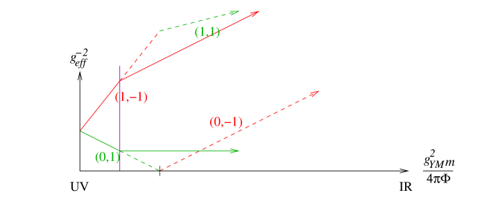
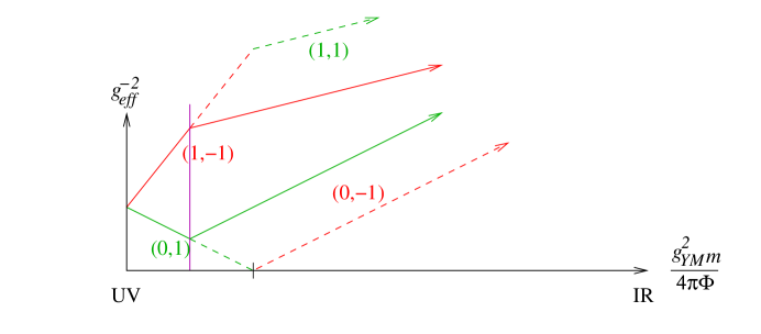
Figure 7: $g_{eff}^{-2}$ from figure 4 modified by enhancon screening with $P=N_{4}$.

Figure 8: $g_{eff}^{-2}$ from figure 4 modified by enhancon screening with $P=2N_{4}$.

For $P=N_{4}$, the modified running of the coupling looks like what is illustrated in figure 8. We can also take $P=2N_{4}$ (assuming $2N_{4}\leq k$), for which the running of coupling looks like figure 8. This latter choice mimics the beta function coefficient of the naive cascade dual. Clearly, there are other possible choice of $P$ that will eliminate the enhancon. Any $P$ in the range

$$N_{4}\leq P\leq N_{4}+{k\over 2}$$ (3.11)

and $\Phi_{s}>\Phi_{e}$ would do. These are by no means intended to be an exhaustive set of enhancon screening configurations. One can easily envision relaxing the ansatz that the D4’s arrange themselves in a spherically symmetric fashion. The point of this exercise is to show that 1) an explicit supergravity solution corresponding to specific points on Coulomb branch like the one we considered is possible in practice, and that 2) there are multitude of enhancon shielding configurations.

Of course, as $\Phi_{s}$ approaches and crosses $\Phi_{e}$, the enhancon returns. The most sensible and conservative interpretation is that any feature encoded in supergravity in the region $\Phi<\Phi_{e}$ when the enhancon is unshielded is unreliable.

It would be gratifying, on the other hand, if the appearance of enhancons when $\Phi_{s}$ approaches $\Phi_{e}$ is signaling that the geometry of the Coulomb branch is modified such that one simply can not un-higgs beyond $\Phi_{s}=\Phi_{e}$. A picture roughly along these lines was suggested by [29] relying mostly on the structure of quantum exact Coulomb branch geometry inferred using the Seiberg-Witten technique. It would be interesting to attempt to close this gap by studying the quantum corrected Coulomb branch geometry for theories in 2+1 dimensions. This issue is currently under investigation and will be reported in a separate publication.

Another interesting question is whether there is a specific supergravity solution (perhaps among the class considered in this article, or its suitable generalization) which corresponds to special points on the Coulomb branch such as the baryonic root [32]. The baryonic root is a point on moduli space and is, in a manner of speaking, the natural one to identify as the “origin” of the Coulomb branch. It is the point where the baryonic branch and the Coulomb branch meet. The branch and geometric structure of the full moduli space and its supergravity manifestation is currently under investigation, which we hope to more thoroughly address in future work.

4 The case of $k=0$

In this section, we will extend the construction and the analysis of the supergravity dual of $U(N)\times U(M)$ theory but with no flavor. Some of these issues was discussed briefly in sections 2.3 and 2.4 of [11] but we will elaborate further on some of the subtleties which were not highlighted there. The $(C^{2}/Z_{2})\times TN_{k}$ geometry at the root of the construction is now modified to $(C^{2}/Z_{2})\times R^{3}\times S^{1}$. The fact that fibration over $S^{1}$ is trivial simplifies issues such as disambiguation of Page, brane, and Maxwell charges. This also implies that the details of charge quantization will be different from what we saw in the previous sections, which one might have anticipated from appearance of various factors of $k^{-1}$. We will encounter various singularities which we will examine in some detail.

When $N=M$, the supergravity solution is simply that of $AdS_{4}\times S^{7}/Z_{2}$. Let us begin by formulating an ansatz for the supergravity solution with some fractional branes present so that $N\neq M$.

We begin with an ansatz in M-theory where we warp the $R^{1,2}\times(C^{2}/Z_{2})\times R^{3}\times S^{1}$ geometry with an ansatz of the form

$$ds^{2}=H^{-2/3}(-dt^{2}+dx_{1}^{2}+dx_{2}^{2})+H^{1/3}(ds^{2}_{C^{2}/Z_{2}}+ds_{R^{3}\times S_{1}}^{2})$$ (4.1)

Unlike the $k\neq 0$ case, we set

$$x^{11}=R_{11}\psi$$ (4.2)

and let $\psi$ have periodicity $2\pi$. We take the ansatz for the M-theory 3-form to be

$$C_{3}=H^{-1}dt\wedge dx_{1}\wedge dx_{2}+C_{3}^{SD}\ ,$$ (4.3)

with

$$C_{3}^{SD}=l\omega_{2}\wedge\left({R_{11}\over 2r}d\psi+\cos\theta d\phi\right)+\alpha\omega_{2}\wedge d\psi$$ (4.4)

The four form field strength

$$G_{4}^{SD}=-l\omega_{2}\wedge\left({R_{11}\over 2r^{2}}dr\wedge d\psi+\sin\theta d\theta\wedge d\phi\right)$$ (4.5)

is self-dual on $(C_{2}/Z_{2})\times R^{3}\times S^{1}$, but is not normalizable. This is the first indication that something subtle is happening. In fact, the equation for the warp factor is the $k\rightarrow 0$ limit of (2.9) and reads

$$0=\left(\nabla^{2}_{y}+\nabla^{2}_{TN}\right)H+{l^{2}\over 2r^{4}}\delta^{4}(\vec{y})+(2\pi l_{p})^{6}Q_{2}\delta^{4}(\vec{y})\delta^{4}(\vec{r})\ ,$$ (4.6)

from which one can immediately infer that the bulk charge

$$\int G_{4}^{SD}\wedge G_{4}^{SD}\sim R_{11}\int d^{3}r\,{l^{2}\over 2r^{4}}$$ (4.7)

diverges near $r=0$. This divergence is addressed by having the enhancon mechanism excise the region near $r=0$, which was how this solution was presented in figure 2 of [11], but it would be nice to see that in a more controlled manner. This is what we will work out in this section. We will in fact see that most of these features are hidden far inside the enhancon radius and is therefore, in many ways, moot.

The reduction to IIA of our ansatz takes the form

$$ds^{2} = H^{-1/2}(-dt^{2}+dx_{1}^{2}+dx_{2}^{2})+H^{1/2}(ds_{ALE}^{2}+ds_{R^{3}}^{2})$$ (4.8)

$$A_{1} = 0$$ (4.9)

$$A_{3} = -(H^{-1}-1)dt\wedge dx_{1}\wedge dx_{2}-l\omega_{2}\wedge\cos\theta d\phi,$$ (4.10)

$$B_{2} = -(2\pi l_{s})^{2}b\omega_{2},\qquad b={1\over(2\pi l_{s})^{2}}\left({l\over r}+{\alpha\over g_{s}l_{s}}\right),$$ (4.11)

$$e^{\phi} = g_{s}H^{1/4}$$ (4.12)

Quantization of D4 charges is rather straight forward. In particular, we find

$$2\pi l=(2\pi l_{s})^{3}g_{s}N_{4},\qquad 2\pi\alpha=g_{s}(2\pi l_{s})^{3}b_{\infty}\ .$$ (4.13)

In terms of $N_{4}$, $b_{\infty}$, $g_{YM}^{2}=g_{s}l_{s}^{-1}$, and $2\pi\Phi=\alpha^{\prime-1}r$ we can write

$$b(r)=b_{\infty}+{g_{YM}^{2}N_{4}\over 2\pi\Phi}$$ (4.14)

which is manifestly dimensionless.

The quantization of D2 charge and its relation to $Q_{2}$ is subtle because of the naively divergent bulk charge (4.7). We can, however, read off the analogue of (2.29) by analyzing the leading derivative term in the expansion of the D4 and anti D4 brane probe DBI action.

$${1\over g_{eff1,2}^{2}(\Phi)}=(n\pm b_{\infty})\mp{g_{YM}^{2}(2N_{4})\over 4\pi\Phi}\ ,$$ (4.15)

which naively leads to the kind of “cascade” illustrated in figure 1.a of [11], except that, as stressed throughout this article, there are no cascades for ${\cal N}=4$ theories in 2+1 dimensions.

To address the issue of relating $Q_{2}$ to quantized charges, it is useful to consider the case of $U(N)\times U(M=N+P)$ at the point on Coulomb branch where gauge group is broken to $U(N)\times U(N)\times U(1)^{P}$ by $P$ fractional branes forming an (approximately) spherical shell at a radius $r_{s}$ in $R^{3}$. In such a setup, one expects the solution for $r<r_{s}$ to precisely be $AdS_{4}\times S^{7}/Z_{2}$ in M-theory, dimensionally reduced to $AdS_{4}\times CP_{3}/Z_{2}$ in IIA with $N=N_{2}$ units of D2 charge. We also expect $l=0$ in the region $r<r_{s}$. At $r=r_{s}$, there are $P$ D4’s each carrying one unit of D4 charge and $b(r_{s})$ units of D2 charge.

In order for $b(r_{s})$ to be a meaningful concept, we need $b(r)$ to be continuous at $r=r_{s}$. That was found to be the case when $k\neq 0$ by requiring the Page and the brane charge to jump by an appropriate amount in the previous section. Here, we do not have the same independent constraint on continuity of $b(r)$, but let us impose that as necessary condition to make the D2 brane charge carried by the $P$ D4-branes well defined.

This then implies that

$$l=\left\{\begin{array}[]{ll}0&(r<r_{s})\\ {1\over 2\pi}(2\pi l_{s})^{3}g_{s}P&(r>r_{s})\end{array}\right.$$ (4.16)

and

$$b(r)=\left\{\begin{array}[]{ll}b_{\infty}-{g_{s}l_{s}P\over r_{s}}&(r<r_{s})\\ b_{\infty}-{g_{s}l_{s}P\over r}&(r>r_{s})\end{array}\right.\ .$$ (4.17)

This spherical shell of D4 at radius $r_{s}$ regulates the bulk charge to

$$2\pi R_{11}\int_{r>r_{s}}d^{3}r{l^{2}\over 2r^{4}}={(2\pi)^{2}l^{2}R\over r}=(2\pi l_{s})^{6}g_{s}^{2}\left({P^{2}g_{s}l_{s}\over r}\right)$$ (4.18)

Note that the sum of D2 brane and bulk charges,

$$Q_{2}^{Maxwell}=N_{2}+b(r_{s})P+{P^{2}R\over r_{s}}=N_{2}+b_{\infty}P$$ (4.19)

is happily independent of $r_{s}$. On the other hand, both the brane charge and the bulk charge diverge as $r_{s}$ approaches zero. Introducing the spherical shell of radius $r_{s}$ is therefore an effective way to regularize this divergence. One can in principle compute the warp factor and consider taking $r_{s}$ to zero. This will then give the same warp factor that was computed in figure 2 of [11] which we reproduce in figure 9.

Figure 9: The solution to the harmonic equation in the decoupling limit, for $k=0$. This figure originally appeared as figure 2 of [11]

There is however one critical issue which requires attention. As one sends $r_{s}$ to zero, the flux of D2 charge at $r=r_{s}$

$$N_{2}+b(r_{s})P=N_{2}+b_{\infty}P-{g_{s}l_{s}P\over r_{s}}$$ (4.20)

turns negative at

$$r_{s}^{*}={g_{s}l_{s}P\over N_{2}+bP}=\alpha^{\prime}{g_{YM}^{2}P\over N_{2}+b_{\infty}P}\ .$$ (4.21)

This is a repulson singularity, and signals that there when $r_{s}<r_{s}^{*}$, one shouldn’t trust the supergravity solution to be capturing the physics of the field theory dual. Note that the scaling with respect to $\alpha^{\prime}$ is such that

$$2\pi\Phi_{s}^{*}={1\over\alpha^{\prime}}r_{s}^{*}={g_{YM}^{2}P\over N_{2}+b_{\infty}P}$$ (4.22)

is finite in the $\alpha^{\prime}\rightarrow 0$ limit.

One can visualize the renormalization group by drawing the cascade-like diagram, for instance, for the case of $N_{2}=7m$ and $N_{4}=4m$ as in figure 12. The region

$${g_{YM}^{2}m\over 4\pi\Phi}>{g_{YM}^{2}m\over 4\pi\Phi_{s}^{*}}={9\over 8}$$ (4.23)

behind the repulson singularity is shaded in grey.

One can shield the repulson singularity by smearing the $P=N_{4}=4m$ D4-branes in a spherical shell with radius

$$\Phi_{s}>\Phi_{s}^{*}$$ (4.24)

as is illustrated in figure 12. It might be tempting to conclude that as long as $\Phi_{s}>\Phi_{s}^{*}$, the supergravity solution is reliably capturing the dynamics of the gauge theory in the gravity dual description.

Figure 10: Cascade-like diagram. Repulson singularity is shaded in gray.

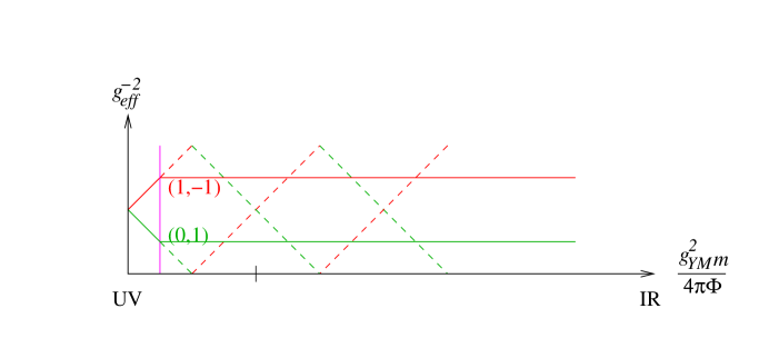
Figure 11: Cascade-like diagram with shielded repulson singularity.

Figure 12: Trustworthy solution with all enhancon radii shielded.

It should be noted, however, that the outer-most enhancon, where one of $g_{eff}^{-1}(\Phi)$ vanishes, occurs at

$${g_{YM}^{2}N_{4}\over 4\pi\Phi_{e}}={b_{\infty}\over 2}={1\over 4}\ .$$ (4.25)

For the same reason as was discussed in the previous section, supergravity solution in the region inside the outer-most enhancon radius should not be considered reliable. In order to obtain a reliable spherically symmetric supergravity solution, we must set the radius $\Phi_{s}$ of the shell to be greater than the enhancon radius $\Phi_{e}$ as is illustrated in figure 12. It may turn out that it simply meaningless to set $\Phi_{s}$ to be smaller than $\Phi_{e}$. It would be interesting to find corroboration to this possibility from the field theory side. At the level of supergravity solution, however, upon setting $\Phi_{s}<\Phi_{e}$, one should treat the region $\Phi_{s}<\Phi<\Phi_{e}$ as unreliable.

One can show that the repulson radius $\Phi_{s}^{*}$ is always smaller than the enhancon radius $\Phi_{e}$. This follows from the inequality

$$2\pi\Phi_{e}={g_{YM}^{2}P\over b_{\infty}}>{g_{YM}^{2}P\over N_{2}+b_{\infty}P}=2\pi\Phi_{s}^{*}$$ (4.26)

or equivalently

$$N_{2}+b_{\infty}P>b_{\infty}$$ (4.27)

which can easily be seen to be always true for $N_{2}>0$, $P>0$, and $0\leq b_{\infty}\leq 1$.

5 Conclusion

In this article, we reviewed the construction [11] of supergravity duals of ${\cal N}=4$ field theories in 2+1 dimensions with gauge group $U(N)\times U(M)$ arising from taking the decoupling limit of brane construction illustrated in figure 1. We then scrutinized the regime of validity of the supergravity solution, and highlighted the fact that

1. an enhancon can appear even in the absence of repulson singularities, such as in the examples illustrated in figures 4 and 5, and

2. at the enhancon radius, supergravity as an effective field theory breaks down because of the existence of tensionless brane objects. As such, the supergravity solution in the region inside the enhancon radius should be considered unreliable.

This implies then that aside from the somewhat restricted class of models satisfying the constraints (2.79) and (2.80), only a small region of the supergravity solution is reliable. In the region where the supergravity ceases to be an effective low energy theory, one expects qualitatively different dynamics than that which is naively implied by the gravity solution. The general expectation is that string and quantum corrections plays an important role. It would be very interesting to verify this expectation on the field theory side, to develop some sense on when and how gravity as an effective theory breaks down in string theory.

We also constructed a generalization of [11] corresponding to specific points on Coulomb branch where the fractional branes are configured in an approximately spherically symmetric distribution (which is reliable in the limit that the number of fractional branes is large.) When the shell of fractional branes is larger than the enhancon radius, all the singularities are screened and the supergravity solution is globally reliable. This then suggests that dynamically interesting things happen as the radius of the shell approaches the enhancon radius. Unfortunately, it is not possible to extract what that dynamics is from gravity alone, but perhaps some information can be extracted from careful consideration of full string theory on one side, and a detailed analysis on the field theory side.

For technical reasons, we restricted our attention to spherically symmetric and smooth distribution of the fractional branes, but solutions corresponding to arbitrary, discrete distribution of the fractional branes should also exist. That is simply an exercise in supergravity. We hope to address this point in the near future. With sufficient higgsing, one expects the enhancons to be shielded, giving rise to a reliable supergravity dual.

A different way to regulate the dynamics of “bad” theories by twisting the geometry to modify the scaling dimension of unitarity violating magnetic monopole operators was suggsted in [37]. It would be interesting to see if a gravity interpretation to the modifications invoked in [37] can be identified, but we leave that question for future work.

Finally, we took a closer look at the case with no flavors. The case without flavor has subtle differences to the flavored case with regards to the details of charge quantization. The solution was found to contain a singularity of a repulson type. This singularity can be screened by higgsing along similar lines as what was done for the flavored case. Nonetheless, the repulson singularity is always surrounded by an enhancon singularity, and since one does not expect supergravity features inside the enhancon radius on general grounds as discussed repeatedly above, we do not expect to attribute much physics to the repulson. On the other hand, one does expect interesting physics, both on field theory and on gravity side, at the outer most enhancon radius.

The issue at the heart of this discussion is the condition for and extent to which the geometry of the region of space-time inside the enhancon is physically meaningful. Closely related issue was discussed, for instance, in [24, 38] where it is argued that as long as some probe can penetrate the region inside the enhancon, the geometry must be reliable. Taking this statement literally, however, would lead to the conclusion that a “bad” theory flows under renormalization group flow to a “good” “Seiberg-dual” which is incompatible with the counting of moduli space. A pragmatic point of view to take for the time being is to interpret the enhancons as a hint that non-trivial dynamics could dramatically correct the classical supergravity expectations, and subject the system to more careful test from both field theory and string theory sides to settle the issue.

One surprising result we find is the mismatch in strength between regularity condition (2.80) on supergravity sidde and (2.81) based on expectation from brane construction. As (2.80) is weaker than (2.81), one can satisfy the former while violating the latter. We believe this is a result of supergravity failing to account for higher curvature or quantum effects despite the fact that there are no obvious indication that supergravity, as an effective theory, is breaking down. This issue clearly deserves further consideration.

It would also be interesting to explore these solutions further, and attempt to construct, to the extent that it is possible, solutions corresponding to these theories at specific but generic points on Higgs and Coulomb branches. It would also be instructive to carefully examine the reliability of supergravity description and compare the results against analysis on field theory side. The amount of supersymmetry and available techniques should allow us to make significant progress in probing these issues further. We plan to report on these findings in future publications.

References

- [1] N. Seiberg and E. Witten, “Gauge dynamics and compactification to three-dimensions,” hep-th/9607163.
- [2] O. Aharony, S. S. Razamat, N. Seiberg, and B. Willett, “ dualities from dualities,” JHEP 1307 (2013) 149, 1305.3924.
- [3] O. Aharony, S. S. Razamat, N. Seiberg, and B. Willett, “3 dualities from 4 dualities for orthogonal groups,” JHEP 1308 (2013) 099, 1307.0511.
- [4] E. Witten, “Supersymmetric index of three-dimensional gauge theory,” hep-th/9903005.
- [5] O. Bergman, A. Hanany, A. Karch, and B. Kol, “Branes and supersymmetry breaking in three-dimensional gauge theories,” JHEP 9910 (1999) 036, hep-th/9908075.
- [6] K. Ohta, “Supersymmetric index and -rule for type IIB branes,” JHEP 9910 (1999) 006, hep-th/9908120.
- [7] T. Suyama, “Supersymmetry breaking in Chern-Simons-matter theories,” JHEP 1207 (2012) 008, 1203.2039.
- [8] G. Giecold, F. Orsi, and A. Puhm, “Insane anti-membranes?,” JHEP 1403 (2014) 041, 1303.1809.
- [9] W. Cottrell, J. Gaillard, and A. Hashimoto, “Gravity dual of dynamically broken supersymmetry,” JHEP 1308 (2013) 105, 1303.2634.
- [10] B. Michel, E. Mintun, J. Polchinski, A. Puhm, and P. Saad, “Remarks on brane and antibrane dynamics,” 1412.5702.
- [11] O. Aharony, A. Hashimoto, S. Hirano, and P. Ouyang, “D-brane Charges in Gravitational Duals of 2+1 Dimensional Gauge Theories and Duality Cascades,” JHEP 1001 (2010) 072, 0906.2390.
- [12] M. Bertolini, P. Di Vecchia, M. Frau, A. Lerda, R. Marotta, and I. Pesando, “Fractional D-branes and their gauge duals,” JHEP 02 (2001) 014, hep-th/0011077.
- [13] C. Closset, Studies of fractional D-branes, in the gauge/gravity correspondence & Flavored Chern-Simons quivers for M2-branes.
- [14] D. Tong, “Three-dimensional gauge theories and ADE monopoles,” Phys. Lett. B448 (1999) 33–36, hep-th/9803148.
- [15] E. Witten, “Branes, instantons, and Taub-NUT spaces,” JHEP 0906 (2009) 067, 0902.0948.
- [16] B. Assel, C. Bachas, J. Estes, and J. Gomis, “Holographic duals of superconformal field theories,” JHEP 1108 (2011) 087, 1106.4253.
- [17] B. Assel, C. Bachas, J. Estes, and J. Gomis, “IIB Duals of Circular Quivers,” JHEP 1212 (2012) 044, 1210.2590.
- [18] S. Mukhi, M. Rangamani, and E. P. Verlinde, “Strings from quivers, membranes from moose,” JHEP 0205 (2002) 023, hep-th/0204147.
- [19] S. A. Cherkis and A. Hashimoto, “Supergravity solution of intersecting branes and AdS/CFT with flavor,” JHEP 0211 (2002) 036, hep-th/0210105.
- [20] C. Bender and S. Orszag, Advanced Mathematical Methods for Scientists and Engineers.
- [21] O. Bergman and S. Hirano, “Anomalous radius shift in ,” JHEP 0907 (2009) 016, 0902.1743.
- [22] C. V. Johnson, A. W. Peet, and J. Polchinski, “Gauge theory and the excision of repulson singularities,” Phys.Rev. D61 (2000) 086001, hep-th/9911161.
- [23] N. Itzhaki, J. M. Maldacena, J. Sonnenschein, and S. Yankielowicz, “Supergravity and the large limit of theories with sixteen supercharges,” Phys.Rev. D58 (1998) 046004, hep-th/9802042.
- [24] J. Polchinski, “ gauge/gravity duals,” Int.J.Mod.Phys. A16 (2001) 707–718, hep-th/0011193.
- [25] I. R. Klebanov and M. J. Strassler, “Supergravity and a confining gauge theory: Duality cascades and SB resolution of naked singularities,” JHEP 0008 (2000) 052, hep-th/0007191.
- [26] N. Seiberg, “Electric - magnetic duality in supersymmetric nonAbelian gauge theories,” Nucl.Phys. B435 (1995) 129–146, hep-th/9411149.
- [27] O. Aharony, “IR duality in supersymmetric and gauge theories,” Phys.Lett. B404 (1997) 71–76, hep-th/9703215.
- [28] O. Aharony, “A note on the holographic interpretation of string theory backgrounds with varying flux,” JHEP 0103 (2001) 012, hep-th/0101013.
- [29] F. Benini, M. Bertolini, C. Closset, and S. Cremonesi, “The cascade revisited and the enhancon bearings,” Phys.Rev. D79 (2009) 066012, 0811.2207.
- [30] N. Seiberg and E. Witten, “Electric - magnetic duality, monopole condensation, and confinement in supersymmetric Yang-Mills theory,” Nucl.Phys. B426 (1994) 19–52, hep-th/9407087.
- [31] N. Seiberg and E. Witten, “Monopoles, duality and chiral symmetry breaking in supersymmetric QCD,” Nucl.Phys. B431 (1994) 484–550, hep-th/9408099.
- [32] P. C. Argyres, M. R. Plesser, and N. Seiberg, “The moduli space of vacua of SUSY QCD and duality in SUSY QCD,” Nucl.Phys. B471 (1996) 159–194, hep-th/9603042.
- [33] A. Hashimoto, P. Ouyang, and M. Yamazaki, “Boundaries and defects of SYM with 4 supercharges. Part I: Boundary/junction conditions,” JHEP 1410 (2014) 107, 1404.5527.
- [34] A. Hashimoto, P. Ouyang, and M. Yamazaki, “Boundaries and defects of SYM with 4 supercharges. Part II: Brane constructions and field theories,” JHEP 1410 (2014) 108, 1406.5501.
- [35] M. Bullimore, T. Dimofte, and D. Gaiotto, “The Coulomb branch of theories,” 1503.04817.
- [36] D. Gaiotto and E. Witten, “S-duality of boundary conditions in super Yang-Mills theory,” Adv.Theor.Math.Phys. 13 (2009) 721, 0807.3720.
- [37] I. Yaakov, “Redeeming bad theories,” JHEP 1311 (2013) 189, 1303.2769.
- [38] C. V. Johnson and R. C. Myers, “The enhancon, black holes, and the second law,” Phys. Rev. D64 (2001) 106002, hep-th/0105159.