High-order Tail in Schwarzschild Space-time

Abstract

We present an analysis of the behaviour at late-times of linear field perturbations of a Schwarzschild black hole space-time. In particular, we give explicit analytic expressions for the field perturbations (for a specific $\ell$-multipole) of general spin up to the first four orders at late times. These expressions are valid at arbitrary radius and include, apart from the well-known power-law tail decay at leading order ($\sim t^{-2\ell-3}$), a new logarithmic behaviour at third leading order ($\sim t^{-2\ell-5}\ln t$). We obtain these late-time results by developing the so-called MST formalism and by expanding the various MST Fourier-mode quantities for small frequency. While we give explicit expansions up to the first four leading orders (for small-frequency for the Fourier modes, for late-time for the field perturbation), we give a prescription for obtaining expressions to arbitrary order within a ‘perturbative regime’.

I Introduction

The study of linear field perturbations of black hole background space-times is important for several purposes. For example, for the investigation of the (linear) stability of black holes, the effect that black holes have on fields propagating in their neighbourhood or the binary inspiral of a black hole and another compact, astrophysical object. In 1955 and subsequent years Regge and Wheeler (1957); Wheeler (1955); Price (1972a, b); Zerilli (1970a, b); Ruffini et al. (1972), the equations describing linear field perturbations of a non-rotating (Schwarzschild) black hole space-time were decoupled and separated. This rendered the equations treatable semi-analytically as the full perturbation may be obtained as a sum of Fourier modes, with the radial part satisfying the so-called Regge-Wheeler (RW) ordinary differential equation. It was not until 1972 that a similar feat was achieved by Teukolsky Teukolsky (1972, 1973) in the case of a rotating (Kerr) black hole space-time. In the Schwarzschild limit, the radial part of the Teukolsky equation reduces to the so-called Bardeen-Press-Teukolsky (BPT) equation Bardeen and Press (1973), which was also obtained in 1972.

The RW and the BPT radial equations are satisfied by different quantities (different combinations of field components and their derivatives) and their solutions have been studied thoroughly, both numerically as well as with asymptotic analyses. Of particular interest for this paper, is the result by Price Price (1972a, b) (obtained by studying the field perturbations without Fourier-decomposing) for the behaviour at late-times of a RW field perturbation of any spin of a Schwarzschild black hole. Price found that its radiative $\ell$-multipole decays to leading-order in the form of a power-law: $t^{-2\ell-3}$, where $t$ the Schwarzschild time. The analysis in hod1998late of the Teukolsky equation in Kerr shows that the same leading-order power-law tail behaviour is satisfied by the radiative multipoles of BPT field perturbations in Schwarzschild. In this paper we present analytic expressions for the behaviour of general-spin field perturbations in Schwarzschild up to the first four orders for late-times, revealing a new logarithmic behaviour in the third leading order ($\sim t^{-2\ell-5}\ln t$). Furthermore, although most analyses (though see, e.g., PhysRevD.61.024026 for an exception) that give the radius-dependent coefficient of the leading-order power-law have been constrained to large radius, our results for all four orders are valid for arbitrary radius. We obtain this late-time behaviour both for the field quantities satisying the RW as well as the BPT equation. We obtain these results by developing a method which is valid not only at late-times, but it may be used to obtain results valid in principle at any time regime. We now briefly introduce this method.

In 1986, Leaver Leaver (1986a) derived various analytical representations for the solutions of the RW and BPT equations in terms of infinite series of special functions. A series of Japanese researchers later ‘revamped’ some of Leaver’s series representations and derived other new series representations for these radial solutions Mano et al. (1996a, b); Sasaki and Tagoshi (2003). These latter series representations, to which we shall refer as MST expansions, are naturally adapted to carrying out small-frequency expansions. Small-frequency expansions yield the late-time behaviour of the full linear perturbation after integration over frequency. We note, however, that the MST series in principle converge for any value of the frequency, although the speed of their convergence decreases as the magnitude of the frequency increases.

The MST method is a powerful method which only relatively recently researchers have been starting to use in order to obtain results in black hole perturbation theory. For example, in the case of a spherically-symmetric background, the MST formalism has found applications in the calculation of the self-force Poisson et al. (2011) on a point particle Hikida et al. (2004, 2005); Casals et al. (2013), post-Newtonian coefficients and gauge-invariant quantities Bini and Damour (2014a, b, c); Shah et al. (2014); Shah (2014) and dynamical tidal interaction of compact objects Delsate et al. (2013). The MST method has proven particularly useful for calculating the retarded Green function (GF) of the wave equation satisfied by the field perturbation, which is a fundamental quantity as it determines the evolution in time of any given initial data. The Fourier modes of the GF posess poles (the so-called quasinormal modes) and a branch cut (BC) in the complex-frequency plane Leaver (1986b). It is known (e.g., Leaver (1986b); Ching et al. (1995a)) that the small-frequency part of the BC is the contribution to the GF that gives rise to the late-time behaviour; the non-small-frequency part of the BC contributes to the behaviour at earlier times (see Casals and Ottewill (2013, 2012a); Casals et al. (2013); Maassen van den Brink (2000, 2004)).

In this paper we derive in detail some of the results on the GF Fourier modes and black hole perturbations that we briefly presented in the Letter Casals and Ottewill (2012b). Namely, we derive a small-frequency expansion of the MST series in general, and of the BC in particular, which we then use to obtain the late-time behaviour of the GF and field perturbations. We obtain the late-time behaviour up to the first four leading orders at arbitrary radius in Schwarzschild space-time and for general-integer-spin of the field. In Casals et al. (2013) we used the calculation of the late-time GF derived in Casals and Ottewill (2012b) in order to find its contribution to the self-force on a scalar charge in Schwarzschild. The MST method has also been used to calculate the quasinormal mode contribution to the GF in Schwarzschild space-time Casals et al. (2013) and in Kerr space-time Zhang et al. (2013); in the former case the GF calculation was applied to obtain the scalar self-force and, in the latter case, to obtain the radiation emitted given a specific perturbation source. The calculations of the quasinormal mode series in Casals et al. (2013); Zhang et al. (2013) involved evaluating the MST series at frequencies with ‘arbitrarily’ large magnitude.

Apart from an explicit small-frequency/late-time analysis, we shall also generally develop the MST formalism in Schwarzschild space-time. In particular, we shall present MST expressions (valid for general frequency) for the solutions of the RW equation for general integer spin. To the best of our knowledge, these expressions are new for spin-1 since the MST formalism has not yet been presented for the RW equation for spin-1 (it only has been for spins-0 and -2). Furthermore, we develop, also for the first time in the literature, the MST formalism for calculating the contribution to the GF of Fourier modes along the BC. We also give the relationships between the BPT quantities and the RW quantities via the so-called Chandrasekhar transformation. We then give explicit expressions for the main MST quantities up to the first four leading orders for small frequency, for general spin and multipole number $\ell$. We note that alhough small-frequency expansions have been given for some of these quantities already, that has typically been done within a post-Newtonian framework, and so for the radial solutions expanded about radial infinity. In here, instead, we give small-frequency expansions for the radial solutions which are valid for arbitrary radius.

For the reader who is not interested in the details and who just wants to use our results in order to obtain the late-time behaviour of the Green function or a field perturbation to high order, the main result is in Sec.VII.1. In particular, in Eq.(141) we give the late-time behaviour of the $\ell$-modes of the GF of the RW equation; above that equation we indicate how to find the coefficients appearing in the equation; below that equation we indicate how to obtain a similar late-time expansion in the BPT case. Of course, if one wants the late-time behaviour of some given initial data for the field perturbation, one should convolute the obtained small-frequency expansions for the GF with the initial data as in Eq.(143).

The layout of this paper is as follows. In Sec.II we present the RW and BPT equations, expressions for their GFs and the BC contributions, as well as the relationships between the RW and BPT quantities. In Sec.III we develop the MST formalism both for the RW and BPT equations, including our new derivation in the specific case of the RW equation for spin-1. In Secs.IV and V we give explicit expansions of the various MST quantities, except for the radial functions, up to the first four leading orders for small frequency. In Sec.VI we extract the small-frequency expansions for the radial functions using a novel method. In Sec.VII we calculate the late-time behaviour of the GF (Sec.VII.1) and of a perturbation response (Sec.VII.2) and compare it with highly-accurate numerical results. In App.A we plot the small-frequency expansions of MST quantities and check that they match with an independent method (presented in Casals and Ottewill (2013)) which is valid in a ‘mid-frequency’ regime. In App.B we relate the radial coefficients of the solutions of the RW and BPT equations.

In this paper we use geometrized units: $c=G=1$. We shall use a bar over a quantity to indicate that the quantity has been made dimensionless via an appropriate factor of ‘$2M$’ (except where otherwise indicated), where $M$ is the black hole mass; e.g., $\bar{\omega}\equiv 2M\omega$ indicates a dimensionless frequency $\omega$ and $\bar{r}\equiv r/(2M)$ a dimensionless Schwarzschild radius $r$.

II Branch cut Green function

II.1 Regge-Wheeler equation

Decoupled and separated equations for linear field perturbations of a Schwarzschild black hole space-time were derived for axial – also called ‘odd’ – gravitational perturbations (spin $s=2$) in Regge and Wheeler (1957), for electromagnetic perturbations ($s=1$) in Wheeler (1955); Ruffini et al. (1972), and for scalar perturbations ($s=0$) in Price (1972a, b). All these integer-spin-field perturbation equations can be written compactly as one single partial differential equation, which in Schwarzschild coordinates reads:

$$\left[\nabla^{\alpha}\nabla_{\alpha}+s^{2}\frac{2M}{r^{3}}\right]\mathcal{X}_{s}=S_{s},$$ (1)

where $\mathcal{X}_{s}=\mathcal{X}_{s}(t,r,\theta,\phi)$ is a scalar function that describes the field perturbation of spin $s$ created by a source $S_{s}$ and

$$\nabla^{\alpha}\nabla_{\alpha}=-\frac{r^{2}}{\Delta}\frac{\partial^{2}}{\partial t^{2}}+\frac{1}{r^{2}}\frac{\partial\ }{\partial r}\left(\Delta\frac{\partial}{\partial r}\right)+\frac{1}{r^{2}\sin\theta}\frac{\partial\ }{\partial\theta}\left(\sin\theta\frac{\partial}{\partial\theta}\right)+\frac{1}{r^{2}\sin^{2}\theta}\frac{\partial}{\partial\phi^{2}}$$ (2)

is the Klein-Gordon operator in Schwarzschild space-time, where $\Delta\equiv r(r-2M)$ and $M$ is the mass of the black hole. Separating variables we may obtain a complete set of solutions of the form

$${}_{s}\mathcal{X}_{\ell m\omega}(t,r,\theta,\phi)=e^{-i\omega t}Y_{\ell m}(\theta,\phi)\frac{{}_{s}X_{\ell m}(r,\omega)}{r},$$ (3)

where $\ell$ and $m$ are, respectively, the multipolar and azimuthal numbers and $Y_{\ell m}(\theta,\phi)$ are the scalar (spin-weight $0$) spherical harmonics. As in Nakano and Sasaki (2001), we treat Eq.(1) as a scalar wave equation, although in the electromagnetic and gravitational cases we have to be aware that the non-radiative ($\ell<|s|$) modes would drop out when constructing the electromagnetic and gravitational potentials and so these modes would have to be included separately. The radial functions satisfy the ordinary differential equation

$$\left[\frac{1}{r^{2}}\frac{\text{d}\ }{\text{d}r}\left(\Delta\frac{\text{d}}{\text{d}r}\right)-2\frac{\Delta}{r^{3}}\frac{\text{d}}{\text{d}r}+\frac{\omega^{2}r^{2}}{\Delta}-\left(\frac{\ell(\ell+1)}{r^{2}}+\frac{2M\left(1-s^{2}\right)}{r^{3}}\right)\right]{}_{s}X_{\ell m}={}_{s}S_{\ell m},$$ (4)

where ${}_{s}S_{\ell m}={}_{s}S_{\ell m}(r,\omega)$ are the corresponding modes of the source $S_{s}$. We shall refer to Eq.(4) as the (radial) Regge-Wheeler (RW) equation and to Eq.(1) as the 4-dimensional RW equation (as per Nakano and Sasaki (2001)). Introducing the standard ‘tortoise’ coordinate $r_{*}\equiv r+2M\ln\bigl{(}r/(2M)-1\bigr{)}$, Eq.(4) may also be written as

$$\left[\frac{\text{d}^{2}\ }{\text{d}r_{*}{}^{2}}+\omega^{2}-\frac{\Delta}{r^{4}}\left(\ell(\ell+1)+\frac{2M\left(1-s^{2}\right)}{r}\right)\right]{}_{s}X_{\ell m}=\frac{\Delta}{r^{2}}{}_{s}S_{\ell m}.$$ (5)

The case of polar – or ‘even’ – gravitational perturbations was derived in Zerilli (1970a, b); the corresponding radial equation is the so-called Zerilli equation. Solutions of the Zerilli equation can be obtained as linear combinations of solutions and their radial derivatives of the RW equation for $s=2$ Chandrasekhar (1983).

We define the retarded Green function (GF) of the 4-dimensional RW Eq.(1) as the solution of Nakano and Sasaki (2001)

$$\left[\nabla^{\alpha}\nabla_{\alpha}+s^{2}\frac{2M}{r^{3}}\right]{}_{s}G_{\text{ret}}(x,x^{\prime})=-\delta(x,x^{\prime})=-\frac{1}{r\,r^{\prime}}\delta(t-t^{\prime})\delta(r-r^{\prime})\delta(\Omega-\Omega^{\prime}),$$ (6)

that obeys appropriate causal boundary conditions, where $x$ and $x^{\prime}$ are two space-time points. Here, $\Omega$ is the solid angle of the 2-sphere. For notational simplicity, we use time translation invariance to henceforth take $t^{\prime}=0$. We may then use the symmetries of the space-time to write

$${}_{s}G_{\text{ret}}(x,x^{\prime})=\frac{1}{r\,r^{\prime}}\int_{-\infty+ic}^{\infty+ic}\frac{d\omega}{2\pi}\sum_{\ell=0}^{\infty}\sum_{m=-\ell}^{\ell}Y_{\ell m}(\theta,\phi)Y^{*}_{\ell m}(\theta^{\prime},\phi^{\prime})\ e^{-i\omega t}{}_{s}G_{\ell}(r,r^{\prime};\omega),$$ (7)

where $c>0$, and the Fourier modes ${}_{s}G_{\ell}(r,r^{\prime};\omega)$ must satisfy

$$\left\{\frac{\text{d}^{2}\ }{\text{d}r_{*}{}^{2}}+\omega^{2}-\frac{\Delta}{r^{4}}\left(\lambda+\frac{2M\left(1-s^{2}\right)}{r}\right)\right\}{}_{s}G_{\ell}(r,r^{\prime};\omega)=-\frac{\Delta}{r^{2}}\delta(r-r^{\prime})=-\delta(r_{*}-r_{*}^{\prime}),$$ (8)

where $\lambda\equiv\ell(\ell+1)$. Correspondingly,

$${}_{s}G_{\ell}(r,r^{\prime};\omega)=-\frac{f_{\ell}(r_{<},\omega)g_{\ell}(r_{>},\omega)}{W\left(\omega\right)},$$ (9)

where $r_{>}\equiv\max(r,r^{\prime})$, $r_{<}\equiv\min(r,r^{\prime})$, and the Wronskian is given by

$$W\left(\omega\right)\equiv W\left[f_{\ell}(r,\omega),g_{\ell}(r,\omega)\right]=f_{\ell}\frac{dg_{\ell}}{dr_{*}}-g_{\ell}\frac{df_{\ell}}{dr_{*}}.$$ (10)

Here, the ‘ingoing’ $f_{\ell}=f_{\ell}(r,\omega)$ and ‘upgoing’ $g_{\ell}=g_{\ell}(r,\omega)$ radial functions are solutions of the homogeneous version of the RW Eq.(5) which, for general spin, behave asymptotically as

$$f_{\ell}\sim\begin{cases}e^{-i\omega r_{*}},&\bar{r}_{*}\to-\infty,\\ A^{in}_{\ell}e^{-i\omega r_{*}}+A^{out}_{\ell}e^{+i\omega r_{*}},&\bar{r}_{*}\to+\infty,\end{cases}$$ (11)

where $\bar{r}_{*}\equiv r_{*}/(2M)$, $A^{in}_{\ell}$ and $A^{out}_{\ell}$ are complex-valued constant coefficients (we give higher-order terms of Eq.(11) in App.B), and

$$g_{\ell}\sim e^{+i\omega r_{*}},\quad\bar{r}_{*}\to+\infty.$$ (12)

It is then easy to see that

$$W=2i\omega A^{in}_{\ell}.$$ (13)

It will be convenient for the next section to define similar ingoing and upgoing solutions of Eq.(5) without choosing a specific overall normalization:

$${}_{s}X^{in}_{\ell}\sim\begin{cases}{}_{s}X^{in,tra}_{\ell}e^{-i\omega r_{*}},&\!\!\!\bar{r}_{*}\to-\infty,\\ {}_{s}X^{in,inc}_{\ell}e^{-i\omega r_{*}}+{}_{s}X^{in,ref}_{\ell}e^{+i\omega r_{*}},&\!\!\!\bar{r}_{*}\to+\infty,\end{cases}$$ (14)

and

$${}_{s}X^{up}_{\ell}\sim\begin{cases}{}_{s}X^{up,inc}_{\ell}e^{+i\omega r_{*}}+{}_{s}X^{up,ref}_{\ell}e^{-i\omega r_{*}},&\!\!\!\bar{r}_{*}\to-\infty,\\ {}_{s}X^{up,tra}_{\ell}e^{+i\omega r_{*}},&\!\!\!\bar{r}_{*}\to+\infty,\end{cases}$$ (15)

where ${}_{s}X^{inc,in/ref/tra}_{\ell}$ and ${}_{s}X^{up,inc/ref/tra}_{\ell}$ are ingoing/reflection/transmission coefficients. It is clear that

$${}_{s}X^{in}_{\ell}={}_{s}X^{in,tra}_{\ell}f_{\ell},\quad{}_{s}X^{up}_{\ell}={}_{s}X^{up,tra}_{\ell}g_{\ell}.$$ (16)

Using the standard spherical harmonic addition theorem, we may now rewrite Eq. (7) as

$${}_{s}G_{\text{ret}}(x,x^{\prime})=\frac{1}{4\pi r\,r^{\prime}}\sum_{\ell=0}^{\infty}(2\ell+1)P_{\ell}(\cos\gamma){}_{s}G^{\text{ret}}_{\ell}(r,r^{\prime};t),$$ (17)

where

$${}_{s}G^{\text{ret}}_{\ell}(r,r^{\prime};t)\equiv\frac{1}{2\pi}\int_{-\infty+ic}^{\infty+ic}d\omega\ {}_{s}G_{\ell}(r,r^{\prime};\omega)e^{-i\omega t},$$ (18)

and $\gamma$ is the angle between the spacetime points $x$ and $x^{\prime}$.

The upgoing radial solution $g_{\ell}$, unlike $f_{\ell}$, possesses a branch cut (BC) in the complex-frequency plane starting at the origin $\omega=0$ and extending down the negative imaginary axis Leaver (1986a, b); Casals and Ottewill (2012b). This BC is inherited by $A^{in}_{\ell}$ and by the Fourier modes ${}_{s}G_{\ell}(r,r^{\prime};\omega)$ of the GF. This BC in $g_{\ell}$, however, only occurs as a change of sign in its imaginary part as the frequency crosses the negative imaginary axis, therefore $|g_{\ell}|$ and $|A^{in}_{\ell}|$ do not possess a BC. We will use a new ‘frequency variable’ $\sigma>0$, so that when $\omega=-i\sigma$ then it lies on the negative imaginary axis and when $\omega=+i\sigma$ then it lies on the positive imaginary axis. We define $\delta A(\bar{\sigma})\equiv A_{+}(-i\bar{\sigma})-A_{-}(-i\bar{\sigma})$ for any function $A=A(\bar{\omega})$ possessing a BC along the NIA, where $A_{\pm}(-i\bar{\sigma})\equiv\lim_{\epsilon\to 0^{+}}A(\pm\epsilon-i\bar{\sigma})$, with $\bar{\sigma}>0$, where $\bar{\sigma}\equiv 2M\sigma$ and $\bar{\omega}\equiv 2M\omega$.

The contribution from the BC to the $\ell$-mode ${}_{s}G^{ret}_{\ell}$ is given by

$${}_{s}G_{\ell}^{BC}(r,r^{\prime};t)\equiv\frac{1}{2\pi i}\int\limits_{0}^{\infty}d\sigma\ \delta{}_{s}G_{\ell}(r,r^{\prime};\sigma)e^{-\sigma t}.$$ (19)

Using the obvious symmetry $g_{\ell}(r,-\omega^{*})=g_{\ell}^{*}(r,\omega)$ together with the boundary condition $g_{\ell}(r,+i\sigma)\sim e^{-\sigma r_{*}}$ as $\bar{r}_{*}\to\infty$ and the fact that all three functions $g_{\ell+}(r,-i\sigma)$, $g_{\ell-}(r,-i\sigma)$ and $g_{\ell}(r,+i\sigma)$ satisfy the same homogenous linear second-order differential equation (namely, the RW equation) with real-valued coefficients along both the negative and the positive imaginary axes (since $\omega=\pm i\sigma$ with $\sigma>0$ there), it follows that

$$\delta g_{\ell}=iq(\sigma)g_{\ell}(r,+i\sigma),$$ (20)

for some real-valued function $q(\sigma)$, and that $W[g_{\ell-}(r,-i\sigma),g_{\ell+}(r,-i\sigma)]=-2i\sigma q(\sigma)$. We refer to $q(\sigma)$ as the ‘BC strength’. The symmetry $f_{\ell}(r,-\omega^{*})=f_{\ell}^{*}(r,\omega)$ together with the fact that $f_{\ell}$ has no BC means that $f_{\ell}(r,-i\sigma)$, with $\sigma>0$, is a real-valued function. Putting all these results together, we find that the discontinuity along the BC of the $\ell$-modes of the GF is given by

$$\delta{}_{s}G_{\ell}(r,r^{\prime};\sigma)\equiv-2i\sigma\frac{q(\sigma)}{\left|W\right|^{2}}f_{\ell}(r,-i\sigma)f_{\ell}(r^{\prime},-i\sigma),$$ (21)

which is a purely-imaginary quantity. The reader may refer to Leung et al. (2003); Casals and Ottewill (2012a) for details.

II.2 Bardeen-Press-Teukolsky equation

The Newman-Penrose formalism offers an alternative way of describing spin-field perturbations of a Schwarzschild black hole background space-time to that provided by the RW formalism (one key advantage of the Newman-Penrose formalism, however, is that it generalizes to Kerr space-time). The scaled Newman-Penrose scalars $\Psi_{s}=\Psi_{s}(t,r,\theta,\phi)$ obey the following equation Bardeen and Press (1973); Teukolsky (1972, 1973):

$$\left\{\nabla^{\alpha}\nabla_{\alpha}+\frac{2s}{r^{2}}\left[\left(-r+\frac{Mr^{2}}{\Delta}\right)\frac{\partial}{\partial t}+(r-M)\frac{\partial}{\partial r}+i\frac{\cos\theta}{\sin^{2}\theta}\frac{\partial}{\partial\phi}+\frac{1-s\cot^{2}\theta}{2}\right]\right\}\Psi_{s}=T_{s},$$ (22)

where $T_{s}$ is the matter source term. The scalings of the Newman-Penrose scalars here are given by

$$\Psi_{s}=\begin{cases}\psi_{0}\ \text{or}\ r^{4}\psi_{4},&s=+2\ \text{or}\ s=-2,\\ \phi_{0}\ \text{or}\ r^{2}\phi_{2},&s=+1\ \text{or}\ s=-1,\\ \varphi,&s=0,\end{cases}$$

where $\psi_{0/4}$ are the radiative Weyl scalars, $\phi_{0/2}$ are the radiative Maxwell scalars and $\varphi$ is a massless scalar field. We note that in the scalar case ($s=0$), Eq.(22) is the same as the 4-dimensional RW Eq.(1).

As for the RW equation Eq.(3), we may obtain a complete set of solutions of Eq.(22) in the form

$$\Psi_{s}(t,r,\theta,\phi)=e^{-i\omega t}{}_{s}Y_{\ell m}(\theta,\phi){}_{s}R_{\ell m}(r,\omega),$$ (23)

where ${}_{s}Y_{\ell m}(\theta,\phi)$ are the spin-weighted spherical harmonics Goldberg et al. (1967); Newman and Penrose (1966). These are given explicitly by ${}_{0}Y_{\ell m}(\theta,\phi)=Y_{\ell m}(\theta,\phi)$,

$${}_{\pm 1}Y_{\ell m}(\theta,\phi) =\frac{1}{\sqrt{\ell(\ell+1)}}\left[\mp\partial_{\theta}-\dfrac{i}{\sin\theta}\partial_{\phi}\right]Y_{\ell m}(\theta,\phi), \ell\geq 1,$$

$${}_{\pm 2}Y_{\ell m}(\theta,\phi) =\frac{1}{\sqrt{(\ell-1)\ell(\ell+1)(\ell+2)}}\left[\partial_{\theta}^{2}-\cot\theta\partial_{\theta}\pm\dfrac{2i}{\sin\theta}\partial_{\theta}\partial_{\phi}\mp\dfrac{2i\cos\theta}{\sin^{2}\theta}\partial_{\theta}\partial_{\phi}-\dfrac{1}{\sin^{2}\theta}\partial_{\phi}^{2}\right]Y_{\ell m}(\theta,\phi), \ell\geq 2.$$ (24)

The spin-weighted spherical harmonics satisfy the following relations:

• the conjugation relation ${}_{s}Y_{\ell m}^{*}(\theta,\phi)=(-1)^{m+s}{}_{-s}Y_{l(-m)}(\theta,\phi)$;

• the orthonormality relation

  $$\int\text{d}^{2}\Omega\>{}_{s}Y_{\ell m}^{*}(\theta,\phi){}_{s}Y_{\ell^{\prime}m^{\prime}}(\theta,\phi)=\delta_{\ell\ell^{\prime}}\delta_{mm^{\prime}};$$

• the completeness relation

  $$\sum\limits_{\ell=|s|}^{\infty}\sum\limits_{m=-\ell}^{\ell}{}_{s}Y_{\ell m}^{*}(\theta,\phi){}_{s}Y_{\ell m}(\theta^{\prime},\phi^{\prime})=\delta(\cos\theta-\cos\theta^{\prime})\delta(\phi-\phi^{\prime});$$

• the parity relation ${}_{s}Y_{\ell m}(\pi-\theta,\pi+\phi)=(-1)^{\ell}{}_{-s}Y_{\ell(-m)}(\theta,\phi)$;

• and the generalised addition relation

  $$\sum_{m}{}_{s_{1}}Y_{\ell m}(\theta,\varphi){}_{s_{2}}Y_{\ell m}^{*}(\theta^{\prime},\varphi^{\prime})=\sqrt{\frac{2l+1}{4\pi}}{}_{s_{1}}Y_{\ell(-s_{2})}(\gamma,\alpha)e^{-is_{1}\beta}$$ (25)

  where

  $$\alpha =\tan^{-1}\left(\cos\theta\sin\theta^{\prime}-\sin\theta\cos\theta^{\prime}\cos(\phi-\phi^{\prime}),-\sin\theta\sin(\phi-\phi^{\prime})\right),$$

  $$\beta =\tan^{-1}\left(\sin\theta\cos\theta^{\prime}-\cos\theta\sin\theta^{\prime}\cos(\phi-\phi^{\prime}),-\sin\theta^{\prime}\sin(\phi-\phi^{\prime})\right).$$

  In particular, when $s_{1}=s_{2}=s$,

  $$\sum_{m}{}_{s}Y_{\ell m}(\theta,\varphi){}_{s}Y_{\ell m}^{*}(\theta^{\prime},\varphi^{\prime})=\frac{2l+1}{4\pi}(-1)^{s}\left(\frac{1+\cos\gamma}{2}\right)^{2s}P_{\ell-s}^{(0,2s)}(\cos\gamma)e^{-is(\alpha+\beta)},$$ (26)

  where $P_{k}^{(a,b)}(x)$ are the Jacobi polynomials.

The radial part of the functions in Eq.(23) satisfies the ordinary differential equation

$$\left[\Delta\frac{\text{d}^{2}}{\text{d}r^{2}}+2(r-M)(s+1)\frac{\text{d}}{\text{d}r}+\left(\frac{\left(r^{2}\omega-2is(r-M)\right)r^{2}\omega}{\Delta}+4is\omega r+s(s+1)-\lambda\right)\right]{}_{s}R_{\ell m}=r^{2}\,{}_{s}T_{\ell m},$$ (27)

where ${}_{s}T_{\ell m}={}_{s}T_{\ell m}(r,\omega)$ are the corresponding modes of the source $T_{s}$. We shall refer to Eq.(27) as the (radial) Bardeen-Press-Teukolsky (BPT) equation and to Eq.(22) as the 4-dimensional BPT equation. We may write the former in self-adjoint form as

$$\left[\frac{\text{d}}{\text{d}r}\Delta^{s+1}\frac{\text{d}}{\text{d}r}+\Delta^{s}\left(\frac{\left(r^{2}\omega-2is(r-M)\right)r^{2}\omega}{\Delta}+4is\omega r+s(s+1)-\lambda\right)\right]{}_{s}R_{\ell m}=r^{2}\Delta^{s}\,{}_{s}T_{\ell m},$$ (28)

or, writing ${}_{s}R_{\ell m}(r,\omega)=(\Delta^{-s/2}/r){}_{s}\chi_{\ell m}(r,\omega)$,

$$\left[\frac{\text{d}^{2}\ }{\text{d}r_{*}^{\,2}}+\omega^{2}+\frac{2is(r-3M)\omega}{r^{2}}-\lambda\frac{\Delta}{r^{4}}-\frac{2M\Delta}{r^{5}}-\frac{M^{2}s^{2}}{r^{4}}\right]{}_{s}\chi_{\ell m}=\frac{\Delta^{s/2+1}}{r}{}_{s}T_{\ell m}.$$ (29)

Let us denote by ${}_{s}\chi_{\ell}$ a general homogeneous solution of Eq. (29). Asymptotically, the homogeneous version of Eq. (29) takes the form

$$\left[\frac{\text{d}^{2}\ }{\text{d}r_{*}^{\,2}}+\left(\omega-is\kappa\right)^{2}\right]{}_{s}\chi_{\ell}\sim 0, \bar{r}_{*}\to-\infty,$$

$$\left[\frac{\text{d}^{2}\ }{\text{d}r_{*}^{\,2}}+\omega^{2}+\frac{2is\omega}{r}\right]{}_{s}\chi_{\ell}\sim 0, \bar{r}_{*}\to+\infty,$$

where $\kappa\equiv 1/(4M)$ and correspondingly the solutions behave (omitting dimensionful constant factors) as linear combinations of

$${}_{s}\chi_{\ell} \sim e^{\pm i\left(\omega-is\kappa\right)r_{*}}\sim e^{\pm s/2}\left(\frac{\Delta}{(2M)^{2}}\right)^{\pm s/2}e^{\pm i\omega r_{*}}, \bar{r}_{*}\to-\infty,$$

$${}_{s}\chi_{\ell} \sim r^{\mp s}e^{\pm i\omega r_{*}}, \bar{r}_{*}\to+\infty.$$

We may define ‘ingoing’ solutions of the homogeneous version of Eq. (29) by their asymptotic behaviour as

$${}_{s}\chi^{in}_{\ell}\sim\begin{cases}{}_{s}R^{in,tra}_{\ell}\left(2M\right)^{1-s}\left(\dfrac{r}{2M}-1\right)^{-s/2}e^{-i\omega r_{*}},&\!\!\!\bar{r}_{*}\to-\infty,\\ {}_{s}R^{in,inc}_{\ell}r^{s}e^{-i\omega r_{*}}+{}_{s}R^{in,ref}_{\ell}r^{-s}e^{+i\omega r_{*}},&\!\!\!\bar{r}_{*}\to+\infty,\end{cases}$$ (30)

and the ‘upgoing’ solutions as

$${}_{s}\chi^{up}_{\ell}\sim\begin{cases}{}_{s}R^{up,inc}_{\ell}\left(2M\right)^{1+s}\left(\dfrac{r}{2M}-1\right)^{s/2}e^{+i\omega r_{*}}+{}_{s}R^{up,ref}_{\ell}\left(2M\right)^{1-s}\left(\dfrac{r}{2M}-1\right)^{-s/2}e^{-i\omega r_{*}},&\!\!\!\bar{r}_{*}\to-\infty,\\ {}_{s}R^{up,tra}_{\ell}r^{-s}e^{+i\omega r_{*}},&\!\!\!\bar{r}_{*}\to+\infty,\end{cases}$$ (31)

for general BPT spin. The corresponding ‘ingoing’ and ‘upgoing’ solutions of the homogeneous version of the BPT Eq.(27) respectively behave asymptotically as

$${}_{s}R^{in}_{\ell}\sim\begin{cases}{}_{s}R^{in,tra}_{\ell}\Delta^{-s}e^{-i\omega r_{*}},&\!\!\!\bar{r}_{*}\to-\infty,\\ {}_{s}R^{in,inc}_{\ell}r^{-1}e^{-i\omega r_{*}}+{}_{s}R^{in,ref}_{\ell}r^{-1-2s}e^{+i\omega r_{*}},&\!\!\!\bar{r}_{*}\to+\infty,\end{cases}$$ (32)

and

$${}_{s}R^{up}_{\ell}\sim\begin{cases}{}_{s}R^{up,inc}_{\ell}e^{+i\omega r_{*}}+{}_{s}R^{up,ref}_{\ell}\Delta^{-s}e^{-i\omega r_{*}},&\!\!\!\bar{r}_{*}\to-\infty,\\ {}_{s}R^{up,tra}_{\ell}r^{-1-2s}e^{+i\omega r_{*}},&\!\!\!\bar{r}_{*}\to+\infty,\end{cases}$$ (33)

where ${}_{s}R_{\ell}^{in,inc/ref/tra}$ are the incidence/reflection/transmission coefficients of the ingoing radial BPT solution; similarly for ${}_{s}R_{\ell}^{up,inc/ref/tra}$ for the upgoing solution. It is convenient to define the following ‘ingoing’ and ‘upgoing’ solutions and coefficients with a hat on, which are normalized with respect to the corresponding transmission coefficients: ${}_{s}\hat{R}^{in}_{\ell}\equiv{}_{s}R^{in}_{\ell}/{}_{s}R^{in,tra}_{\ell}$, ${}_{s}\hat{R}^{up}_{\ell}\equiv{}_{s}R^{up}_{\ell}/{}_{s}R^{up,tra}_{\ell}$, ${}_{s}\hat{R}^{in,inc}_{\ell}\equiv{}_{s}R^{in,inc}_{\ell}/{}_{s}R^{in,tra}_{\ell}$. Then it is easy to see that

$$W^{T}(\omega)\equiv W^{T}\left[{}_{s}\hat{R}^{in}_{\ell},{}_{s}\hat{R}^{up}_{\ell}\right]\equiv\Delta^{s+1}\left({}_{s}\hat{R}^{in}_{\ell}{}_{s}\hat{R}^{up^{\prime}}_{\ell}-{}_{s}\hat{R}^{up}_{\ell}{}_{s}\hat{R}^{in^{\prime}}_{\ell}\right)=2i\omega{}_{s}\hat{R}^{in,inc}_{\ell},$$ (34)

where primes denote differentiation wrt $r$. The quantity $W^{T}$ is a ‘generalized Wronskian’ in the sense that it is independent of $r$. Similarly to the RW case, the solution ${}_{s}\hat{R}^{up}_{\ell}$ has a BC along the negative imaginary axis of the complex frequency plane, which is inherited by $W^{T}$, whereas ${}_{s}\hat{R}^{in}_{\ell}$ has no BCs Leaver (1986a).

The GF of the $4$-dimensional BPT equation is the solution of Eq.(22) with the source $T_{s}$ replaced by the distribution $\delta(r-r^{\prime})\delta(\cos\theta-\cos\theta^{\prime})\delta(\phi-\phi^{\prime})/\sqrt{-g}$. It may be expressed as

$${}_{s}G_{\text{ret},T}(x,x^{\prime})=\sum_{\ell,m}\Delta^{s}(r^{\prime}){}_{s}G^{\text{ret},T}_{\ell}(r,r^{\prime};t){}_{s}Y_{\ell m}(\theta,\varphi){}_{s}Y_{\ell m}^{*}(\theta^{\prime},\varphi^{\prime}),$$ (35)

where

$${}_{s}G^{\text{ret},T}_{\ell}(r,r^{\prime};t)\equiv\int_{-\infty+ic}^{\infty+ic}d\omega\ {}_{s}G^{T}_{\ell}(r,r^{\prime};\omega)e^{-i\omega t},\quad{}_{s}G^{T}_{\ell}(r,r^{\prime};\omega)\equiv-\frac{{}_{s}\hat{R}^{in}_{\ell}(r_{<},\omega){}_{s}\hat{R}^{up}_{\ell}(r_{>},\omega)}{W^{T}(\omega)}.$$

In order to obtain an expression for the BC contribution ${}_{s}G_{\ell}^{BC,T}$ to the $\ell$-mode ${}_{s}G^{\text{ret},T}_{\ell}$ of the GF of the $4$-dimensional BPT equation we proceed similarly to the previous subsection for the RW equation. This contribution can be expressed as in Eq.(21) for the RW case, but with ${}_{s}G_{\ell}^{BC}$ and $\delta{}_{s}G_{\ell}$ replaced by ${}_{s}G_{\ell}^{BC,T}$ and $\delta{}_{s}G^{T}_{\ell}$, respectively. We then note that ${}_{s}\hat{R}^{up}_{\ell}(r,-\omega^{*})={}_{s}\hat{R}^{up^{*}}_{\ell}(r,\omega)$ and that $\Delta^{-s}{}_{-s}\hat{R}^{up}_{\ell}(r,+i\sigma)$ goes like $e^{-\sigma r_{*}}/r$ as $\bar{r}\to\infty$ (neglecting a constant factor). It can be shown that all three functions ${}_{s}\hat{R}^{up}_{\ell+}(r,-i\sigma)$, ${}_{s}\hat{R}^{up}_{\ell-}(r,-i\sigma)$ and $\Delta^{-s}{}_{-s}\hat{R}^{up}_{\ell}(r,+i\sigma)$ satisfy the same homogenous linear second-order differential equation (namely, the BPT equation) with real-valued coefficients along the imaginary-$\omega$ axis (since $\omega=\pm i\sigma$ with $\sigma>0$ there). The two former solutions have the same large-$\bar{r}$ behaviour, which is linearly independent from that of the latter. Therefore, it follows that

$$\delta{}_{s}\hat{R}^{up}_{\ell}=iq^{T}(\sigma)\Delta^{-s}{}_{-s}\hat{R}^{up}_{\ell}(r,+i\sigma),$$ (36)

for some real-valued function $q^{T}(\sigma)$, and that $W^{T}\left[{}_{s}\hat{R}^{up}_{\ell-},{}_{s}\hat{R}^{up}_{\ell+}\right]=-2i\sigma q^{T}(\sigma)$. We emphasize that the ‘BC strength’ function $q^{T}$ is calculated using the ‘upgoing’ radial function along the positive imaginary axis with the opposite spin-sign, as opposed to the same spin-sign for calculating $q$ in the RW case (see Eq.(20)). The property ${}_{s}\hat{R}^{in}_{\ell}(r,-\omega^{*})={}_{s}\hat{R}^{in^{*}}_{\ell}(r,\omega)$ together with the fact that ${}_{s}\hat{R}^{in}_{\ell}$ has no BC means that ${}_{s}\hat{R}^{in}_{\ell}(r,-i\sigma)$, with $\sigma>0$, is a real-valued function. Putting all these results and properties together, we find that the discontinuity along the BC of the $\ell$-modes of the $4$-dimensional BPT GF is given by

$$\delta{}_{s}G^{T}_{\ell}(r,r^{\prime};\sigma)=-2i\sigma\frac{q^{T}(\sigma)}{\left|W^{T}\right|^{2}}{}_{s}\hat{R}^{in}_{\ell}(r,-i\sigma){}_{s}\hat{R}^{in}_{\ell}(r^{\prime},-i\sigma).$$ (37)

In the next subsection we relate the BPT quantities to the RW quantities and, in particular, we present an alternative way (namely via the RW ‘BC strength’ $q(\sigma)$) of calculating the BPT discontinuity $\delta{}_{s}G^{T}_{\ell}$.

II.3 Relationship between RW and BPT quantities

The so-called Chandrasekhar transformation relates, in the homogeneous case, solutions of the RW equation to solutions of the BPT equation. We note that while the RW Eqs.(1) and (4) are symmetric under $s\leftrightarrow-s$, the BPT Eqs.(22) and (27) are not. We here write the Chandrasekhar transformation compactly for spin $s=0,-1,-2$ (see Chandrasekhar (1975) for spin-2 and, e.g. Jensen et al. (1991) for spin-1; there are similar transformations in the case of positive spin – which of course only changes the BPT equation, not the RW equation – but we do not deal with these in this paper).

Let us generically denote by ${}_{s}\mathcal{X}_{\ell}(t,r)$ a homogeneous solution of the 4-D RW Eq.(1) after factorizing out the angle-dependence via scalar spherical harmonics; similarly, we generically denote by ${}_{s}\Psi_{\ell}(t,r)$ a homogeneous solution of the 4-D BPT Eq.(22) after factorizing out the angle-dependence via spin-weighted spherical harmonics. The corresponding Chandrasekhar transformation is then Nakano and Sasaki (2001):

$${}_{s}\Psi_{\ell}(t,r) =\mathcal{O}(t,r){}_{s}\mathcal{X}_{\ell}(t,r),\quad\mathcal{O}(t,r)\equiv\left(\frac{\Delta}{r}\right)^{|s|}\left(\partial_{r}-\frac{r^{2}}{\Delta}\partial_{t}\right)^{|s|}r^{|s|-1},$$ (38)

up to a normalization constant. We already gave in Eq.(24) the angular counterpart of the above transformation, i.e., the transformation from the angular factor in the 4-D RW $\ell$-modes (namely, the scalar spherical harmonics) to the angular factor in the 4-D BPT $\ell$-modes (namely, the spin-weighted spherical harmonics). We note that if Eq.(24) were naively applied to the modes $\ell<|s|$ it would yield the zero function.

It is useful to write the Chandrasekhar transformation in the frequency domain explicitly for each spin $s=0$, $-1$ and $-2$ separately. We now generically denote by ${}_{s}X_{\ell}$ and ${}_{s}R_{\ell}$ homogeneous solutions to the (radial) RW Eq.(4) and (radial) BPT Eq.(27), respectively. Introducing the operators

$$\mathcal{D}\equiv\frac{\text{d}\ }{\text{d}r}+\frac{i\omega}{f(r)},\qquad\mathcal{D}^{\dagger}=\frac{\text{d}\ }{\text{d}r}-\frac{i\omega}{f(r)},$$

where $f(r)\equiv\Delta/r^{2}$, we may express the BPT solutions in terms of the RW solutions as

$${}_{0}R_{\ell} =\frac{c_{0}}{r}{}_{0}X_{\ell},$$ (39)

$${}_{-1}R_{\ell} =c_{1}(r-2M)\mathcal{D}{}_{-1}X_{\ell}=c_{1}r\left[f(r){}_{-1}X_{\ell}^{\prime}+i\omega{}_{-1}X_{\ell}\right],$$

$${}_{-2}R_{\ell} =c_{2}(r-2M)^{2}\mathcal{D}{}^{2}\bigl{(}r{}_{-2}X_{\ell}\bigr{)}$$

$$=c_{2}\left[2(ir^{2}\omega+r-3M)r(f(r){}_{-2}X_{\ell}^{\prime}+i\omega{}_{-2}X_{\ell})+(\ell(\ell+1)r-6M)f(r){}_{-2}X_{\ell}\right],$$

where $c_{0}$, $c_{1}$ and $c_{2}$ are constants of proportionality and primes denote differentiation with respect to $r$. Conversely, we have

$${}_{0}X_{\ell} =\frac{1}{c_{0}}r{}_{0}R_{\ell},$$ (40)

$${}_{-1}X_{\ell} =\frac{1}{\lambda c_{1}}r^{2}\mathcal{D}^{\dagger}\left(\frac{{}_{-1}R_{\ell}}{r}\right)=\frac{1}{\lambda c_{1}}\left[r{}_{-1}R_{\ell}^{\prime}-\left(1+\frac{i\omega r}{f(r)}\right){}_{-1}R_{\ell}\right],$$

$${}_{-2}X_{\ell} =\frac{1}{\bigl{(}(\ell-1)\ell(\ell+1)(\ell+2)-12iM\omega\bigr{)}c_{2}}r^{3}\mathcal{D}^{\dagger\,2}\left(\frac{{}_{-2}R_{\ell}}{r^{2}}\right)$$

$$=\frac{1}{\bigl{(}(\ell-1)\ell(\ell+1)(\ell+2)-12iM\omega\bigr{)}c_{2}}\left[\frac{2(3M-r-i\omega r^{2})}{r-2M}{}_{-2}R_{\ell}^{\prime}+\right.$$

$$\qquad\qquad\left.\frac{r^{2}\left(\ell(\ell+1)-2r^{2}\omega^{2}+8i\omega r+4\right)-2Mr\left(\ell(\ell+1)+9i\omega r+10\right)+24M^{2}}{r(r-2M)^{2}}{}_{-2}R_{\ell}\right].$$

We will now use the Chandrasekhar transformation in order to relate the BPT and RW Wronskians as well as the BPT and RW ‘BC strengths’. The specific normalizations (11) and (12) of the RW radial functions $f_{\ell}$ and $g_{\ell}$ yield specific normalizations for the corresponding BPT radial functions via the transformation Eq(38). We will denote the BPT radial functions and coefficients with these specific normalizations with a tilde superscript, i.e., ${}_{s}\tilde{R}^{in}_{\ell}\equiv\mathcal{O}_{\omega}(r)f_{\ell}$, ${}_{s}\tilde{R}^{up}_{\ell}\equiv\mathcal{O}_{\omega}(r)g_{\ell}$ and ${}_{s}\tilde{R}^{in,tra}_{\ell}$, ${}_{s}\tilde{R}^{up,tra}_{\ell}$, …are, respectively, the coefficients ${}_{s}R^{in,tra}_{\ell}$, ${}_{s}R^{up,tra}_{\ell}$, …  of ${}_{s}\tilde{R}^{in}_{\ell}$ and ${}_{s}\tilde{R}^{up}_{\ell}$. In App.B we use the Chandrasekhar transformation in order to find these BPT radial coefficients and Wronskian in terms of the RW radial coefficients and Wronskian. We are here using the obvious notation of $\mathcal{O}_{\omega}(r)$ for $\mathcal{O}(t,r)$ after replacing ‘$\partial_{t}$’ by ‘$-i\omega$’ in it.

Let us now try to find an alternative expression to Eq.(37) for the BPT $\delta{}_{s}G^{T}_{\ell}$ in terms of the RW $q(\sigma)$. We first re-express the BPT modes ${}_{s}G^{T}_{\ell}$ of Eq.(35) in terms of the RW solutions $f_{\ell}$ and $g_{\ell}$ by using the Chandrasekhar transformation Eq.(38):

$${}_{s}G^{T}_{\ell}(r,r^{\prime};\sigma)=-\mathcal{O}_{\omega}(r_{<})\mathcal{O}_{\omega}(r_{>})\frac{f_{\ell}(r_{<},\omega)g_{\ell}(r_{>},\omega)}{{}_{s}\tilde{R}^{in,tra}_{\ell}{}_{s}\tilde{R}^{up,tra}_{\ell}W^{T}}.$$ (41)

Using this expression we can find the discontinuity of the BPT $\ell$-modes as

$$\delta{}_{s}G^{T}_{\ell}(r,r^{\prime};\sigma)=\frac{W}{{}_{s}\tilde{R}^{in,tra}_{\ell}{}_{s}\tilde{R}^{up,tra}_{\ell}W^{T}}\mathcal{O}_{\omega}(r)\mathcal{O}_{\omega}(r^{\prime})\delta{}_{s}G_{\ell}(r,r^{\prime};\sigma)=-\frac{2i\sigma q(\sigma){}_{s}\tilde{R}^{in,tra}_{\ell}}{W^{T}\cdot W^{*}{}_{s}\tilde{R}^{up,tra}_{\ell}}{}_{s}\hat{R}^{in}_{\ell}(r,\omega){}_{s}\hat{R}^{in}_{\ell}(r^{\prime},\omega).$$ (42)

In deriving Eq.(42) we have used the fact that $W/({}_{s}\tilde{R}^{in,tra}_{\ell}\cdot{}_{s}\tilde{R}^{up,tra}_{\ell}W^{T})$ does not have a BC (as can be seen from the expressions in App.B) and we have made use of Eq.(21).

Comparing Eqs.(37) and (42) we immediately obtain a relationship between the RW and BPT ‘BC strengths’:

$$q^{T}(\sigma)=\left(\frac{W^{T}}{W}\right)^{*}\cdot\frac{{}_{s}\tilde{R}^{in,tra}_{\ell}}{{}_{s}\tilde{R}^{up,tra}_{\ell}}q(\sigma).$$ (43)

Using the results in App.B, we have that

$$q^{T}(\sigma)=q(\sigma)\begin{cases}1&s=0,\\ \displaystyle-\frac{\alpha^{*}_{\infty}\alpha_{+}}{2\sigma\alpha_{+}^{*}},&s=-1,\\ \displaystyle\frac{\beta_{\infty}^{*}(\alpha_{+}+2M^{2}\beta_{+})}{2\sigma^{2}(\alpha^{*}_{+}+2M^{2}\beta^{*}_{+})},&s=-2,\end{cases}$$ (44)

and

$$\frac{q^{T}}{|W^{T}|^{2}}=\frac{{}_{s}\tilde{R}^{in,tra}_{\ell}}{{}_{s}\tilde{R}^{up,tra}_{\ell}}\frac{W}{W^{T}}\frac{q}{|W|^{2}}=\frac{q}{|W|^{2}}\begin{cases}\frac{1}{4M^{2}}&s=0,\\ \displaystyle-\frac{\alpha_{+}^{2}}{2\sigma\alpha_{\infty}},&s=-1,\\ \displaystyle\frac{(\alpha_{+}+2M^{2}\beta_{+})^{2}}{2M^{2}\sigma^{2}\beta_{\infty}},&s=-2.\end{cases}$$ (45)

Inverting the relationship and using the results in App.B, we explicitly obtain:

$$\frac{q}{|W|^{2}}=\mathcal{C}\frac{q^{T}}{|W^{T}|^{2}}$$ (46)

with

$$\mathcal{C} =4M^{2}, s=0,$$ (47)

$$\mathcal{C} =-\frac{16\lambda M^{4}}{\left(\lambda-s^{2}+1\right)^{2}}\left(1-4\bar{\sigma}+4\bar{\sigma}^{2}\right), s=-1,$$

$$\mathcal{C} =\frac{256M^{6}(1-2\bar{\sigma})^{2}(1-\bar{\sigma})^{2}}{\lambda^{2}-2\lambda-6\bar{\sigma}}, s=-2.$$

The small-frequency behaviour of $\mathcal{C}$ for $s=0$ and $-1$ is already manifest in the exact result above; for $s=-2$ we expand it as

$$\mathcal{C}=\frac{256M^{6}}{(\lambda-2)\lambda}\left(1-\frac{6\left(\lambda^{2}-2\lambda-1\right)\bar{\sigma}}{(\lambda-2)\lambda}+\frac{\left(13\lambda^{4}-52\lambda^{3}+16\lambda^{2}+72\lambda+36\right)\bar{\sigma}^{2}}{(\lambda-2)^{2}\lambda^{2}}\right)+O\left(\bar{\sigma}^{3}\right),\quad s=-2.$$ (48)

From Eqs.(37), (46) and the fact that the radial functions $f_{\ell}$ and ${}_{s}\hat{R}^{in}_{\ell}$ are generically of the same leading order (order zero) in $\bar{\sigma}$ as $\bar{\sigma}\to 0$ (see Secs.IIIVI), it follows that the RW and the BPT BC modes $\delta{}_{s}G_{\ell}$ and $\delta{}_{s}G^{T}_{\ell}$ are of the same leading order in $\bar{\sigma}$ as $\bar{\sigma}\to 0$. As a consequence, the RW and BPT GFs are of the same leading order in $\bar{t}$ as $\bar{t}\to\infty$, as we explicitly see in Sec.VII. That is, the RW and the BPT quantities describing black hole perturbations decay at the same rate at late times.

III MST formalism for the RW and BPT equations for general spin

The MST method for the Teukolsky equation in Kerr (and, therefore, for the BPT equation in Schwarzschild) was given in ST for general spin, and earlier in Mano et al. (1996a) (henceforth MSTa) just for spin-2. To the best of our knowledge, however, the MST method for the RW equation has only been given for spin-2, which was done in Mano et al. (1996b) (henceforth MSTb). Therefore, the MST method for the RW equation still has not been developed for spin-1 (obviously, the RW spin-0 case is essentially just the same as in ST with $s=0$). In this section, we develop the MST method for the RW equation for general spin: for spin-2 we recover MSTb, for spin-0 we essentially recover ST with $s=0$ and, for spin-1, to the best of our knowledge, the results are new. We also develop the MST method for the BPT equation which, although already existing in the literature, will allow us to emphasise the connections between the MST formalism for the RW and BPT equations for general spin $s=0$, $-1$ and $-2$. In particular, we write the expansions for the radial solutions of both the RW and BPT equations in terms of just one set of ‘universal’ coefficients (namely, $a_{n}$). When referring to the literature, we shall use the generic term MST to refer to all MSTa, MSTb and ST.

We shall we use the notation of $X^{\text{in/up}}_{s}$ and $R_{s}^{\text{in/up}}$ (i.e., with a slight change in the subindices with respect to the homogeneous RW solutions ${}_{s}X^{in/up}_{\ell}$ and the BPT solutions ${}_{s}R^{in/up}_{\ell}$, respectively) for the ingoing/upgoing solutions of the RW and BPT equations when using the specific normalization as in MST (i.e., the one in Eqs.(60) and (68) below). A similar change in the subindices notation applies to their incidence, reflection and transmission coefficients.

III.1 Series of hypergeometric functions

In this section we shall assume that $s\leq 0$. For the RW functions we write

$$X^{\text{in}}_{s}=e^{i\bar{\omega}}\bar{r}^{s+1}e^{-i\omega r_{*}}\check{p}_{s}^{\text{in}}(x)=\bar{r}^{s+1}e^{-i\bar{\omega}(\bar{r}-1)}\left(\bar{r}-1\right)^{-i\bar{\omega}}\check{p}_{s}^{\text{in}}(x)=(1-x)^{s+1}e^{i\bar{\omega}x}\left(-x\right)^{-i\bar{\omega}}\check{p}_{s}^{\text{in}}(x),$$ (49)

where $x\equiv 1-\bar{r}$. This leads to the ordinary differential equation

$$x(1-x)\check{p}_{s}^{\text{in}}{}^{\prime\prime}(x)+\bigl{(}1-2i\bar{\omega}(1-x)^{2}-2(1+s)x\bigr{)}\check{p}_{s}^{\text{in}}{}^{\prime}(x)$$ (50)

$$\qquad\qquad+\bigl{(}(\ell-s)(\ell+s+1)+2i\bar{\omega}(1+s)(1-x)\bigr{)}\check{p}_{s}^{\text{in}}(x)=0.$$

Correspondingly, for the BPT functions we write (as in ST)

$$R_{s}^{\text{in}}=e^{i\bar{\omega}}\left(\bar{r}-1\right)^{-s}e^{-i\omega r_{*}}p_{s}^{\text{in}}(x)=e^{-i\bar{\omega}(\bar{r}-1)}\left(\bar{r}-1\right)^{-s-\bar{\omega}i}p_{s}^{\text{in}}(x)=e^{i\bar{\omega}x}\left(-x\right)^{-s-\bar{\omega}i}p_{s}^{\text{in}}(x),$$

which leads to the equation

$$x(1-x)p_{s}^{\text{in}}{}^{\prime\prime}(x)+\bigl{(}4iM\omega x(1-x)+2(2iM\omega-1)x+(1-s-4iM\omega)\bigr{)}p_{s}^{\text{in}}{}^{\prime}(x)$$ (51)

$$\qquad\qquad+\bigl{(}\ell(\ell+1)+4iM\omega(1-s)(1-x)\bigr{)}p_{s}^{\text{in}}(x)=0.$$

In terms of $\check{p}_{s}^{\text{in}}(x)$ and $p_{s}^{\text{in}}(x)$ the Chandrasekhar transformations take the form

$$p_{0}^{\text{in}}(x) =c_{0}\check{p}_{0}^{\text{in}}(x),$$

$$p_{-1}^{\text{in}}(x) =c_{1}\check{p}_{-1}^{\text{in}}{}^{\prime}(x),$$

$$p_{-2}^{\text{in}}(x) =c_{2}\check{p}_{-2}^{\text{in}}{}^{\prime\prime}(x),$$

and conversely

$$\check{p}_{0}^{\text{in}}(x) =\frac{1}{c_{0}}p_{0}^{\text{in}}(x),$$

$$\check{p}_{-1}^{\text{in}}(x) =\frac{1}{\ell(\ell+1)c_{1}}\left[x(1-x)p_{-1}^{\text{in}}{}^{\prime}(x)+\left(1-2i\bar{\omega}(1-x)^{2}\right)p_{-1}^{\text{in}}(x)\right],$$

$$\check{p}_{-2}^{\text{in}}(x) =\frac{1}{\bigl{(}(\ell-1)\ell(\ell+1)(\ell+2)-6i\bar{\omega}\bigr{)}c_{2}}\left[x(1-x)\left(2x+1-2i\bar{\omega}(1-x)^{2}\right)p_{-2}^{\text{in}}{}^{\prime}(x)\right.$$

$$\qquad\left.-\left(\ell(\ell+1)x(1-x)+4\bar{\omega}^{2}(1-x)^{4}+6i\bar{\omega}(x+1)(1-x)^{2}-2(2x+1)\right)p_{-2}^{\text{in}}(x)\right].$$

We now follow MST and introduce the expansion in terms of hypergeometric functions,

$$\check{p}_{s}^{\text{in}}(x) =N_{s}^{\text{in}}\sum_{n=-\infty}^{\infty}\check{a}_{n}\frac{\Gamma(-n-\nu+s-i\bar{\omega})\Gamma(n+\nu+s+1-i\bar{\omega})}{\Gamma(1-2i\bar{\omega})}\times$$

$$\qquad\qquad\qquad\qquad\,{}_{2}F_{1}(-n-\nu+s-i\bar{\omega},n+\nu+s+1-i\bar{\omega};1-2i\bar{\omega};x),$$ (52a)

$$p_{s}^{\text{in}}(x) =N_{s}^{\text{in}}\sum_{n=-\infty}^{\infty}a_{n}\frac{\Gamma(-n-\nu-i\bar{\omega})\Gamma(n+\nu+1-i\bar{\omega})}{\Gamma(1-s-2i\bar{\omega})}\times$$

$$\qquad\qquad\qquad\qquad\,{}_{2}F_{1}(-n-\nu-i\bar{\omega},n+\nu+1-i\bar{\omega};1-s-2i\bar{\omega};x),$$ (52b)

where $N_{s}^{\text{in}}$ is a normalization constant which we specify later on. Here, the parameter $\nu$ is referred to as the renormalized angular momentum and is determined by the requirement that these series converge both as $n\to\infty$ and $n\to-\infty$, it has the property that either $\nu=\ell+O(\bar{\omega})$ or $\nu=-\ell-1+O(\bar{\omega})$; see MSTa or ST for a full discussion. These series representations in terms of hypergeometric functions converge $\forall r\in[2M,\infty)$.

In these terms, the Chandrasekhar transformations follow from the standard identity (Eq.15.5.1 DLMF )

$$\frac{\text{d}\ }{\text{d}x}\,_{2}F_{1}(a,b;c;x)=\frac{ab}{c}\,_{2}F_{1}(a+1,b+1;c+1;x),$$

for some parameters $a$, $b$ and $c$. Inserting into their respective differential equations and using the standard hypergeometric function identities

$$x\,_{2}F_{1}(a,b;c;x)=\frac{a(b-c)}{(a-b)(a-b+1)}\,_{2}F_{1}(a+1,b-1;c;x)+$$

$$\qquad\qquad\qquad\frac{c(a+b-1)-2ab}{(a-b-1)(a-b+1)}\,_{2}F_{1}(a,b;c;x)+\frac{b(a-c)}{(a-b-1)(a-b)}\,_{2}F_{1}(a-1,b+1;c;x),$$

$$x(1-x)\frac{\text{d}\ }{\text{d}x}\,_{2}F_{1}(a,b;c;x)=\frac{ab(c-b)}{(a-b)(a-b+1)}\,_{2}F_{1}(a+1,b-1;c;x)+$$

$$\qquad\qquad\qquad\frac{ab(2c-a-b-1)}{(a-b+1)(a-b-1)}\,_{2}F_{1}(a,b;c;x)+\frac{ab(a-c)}{(a-b)(a-b-1)}\,_{2}F_{1}(a-1,b+1;c;x),$$

we find that $\check{a}_{n}$ and $a_{n}$ must satisfy the same three-term recurrence relation:

$$\alpha_{n}a_{n+1}+\beta_{n}a_{n}+\gamma_{n}a_{n-1}=0,$$ (53)

where

$$\alpha_{n} =-\frac{i\bar{\omega}(n+\nu+1-i\bar{\omega})(n+\nu+1+s-i\bar{\omega})(n+\nu+1+s+i\bar{\omega})(n+\nu)}{(2n+2\nu+3)},$$

$$\beta_{n} =-\mathcal{\lambda}(n+\nu)(n+\nu+1)+\bigl{(}(n+\nu)(n+\nu+1)+\bar{\omega}^{2}\bigr{)}^{2}+s^{2}\bar{\omega}^{2},$$

$$\gamma_{n} =\frac{i\bar{\omega}(n+\nu+i\bar{\omega})(n+\nu-s+i\bar{\omega})(n+\nu-s-i\bar{\omega})(n+\nu+1)}{(2n+2\nu-1)}.$$

The overall normalisation of the coefficients in the homogeneous Eq.(53) is, of course, irrelevant for the value of the $a_{n}$ but the above form has the advantage that all denominators are bounded away from 0 in the perturbative (small-frequency) regime. By ‘perturbative regime’ we essentially mean the frequency regime where $\nu$ is real – see the end of Sec.IV for further details. We choose the normalization $\check{a}_{0}=a_{0}=1$, so then we have $\check{a}_{n}=a_{n}$, $\forall n\in\mathbb{Z}$, and from now on we will write down all series using the ‘universal’ set of coefficients $a_{n}$. These coefficients $a_{n}$ are equal, for $s=-2$, to the $a_{n}^{\nu}$ in MSTb as long as the same normalization is chosen for the two sets.

We could alternatively choose to include the $\Gamma$-functions in the coefficients, that is, write

$$a_{n}^{\text{RW}} \propto a_{n}\frac{\Gamma(-n-\nu+s-i\bar{\omega})\Gamma(n+\nu+s-i\bar{\omega}+1)}{\Gamma(1-2i\bar{\omega})},$$ (54)

$$a_{n}^{\text{T}} \propto a_{n}\frac{\Gamma(-n-\nu-i\bar{\omega})\Gamma(n+\nu-i\bar{\omega}+1)}{\Gamma(1-s-2i\bar{\omega})},$$ (55)

where the constants of proportionality are independent of $n$ and so just reflect the normalisation of the series. A particularly convenient choice is

$$a_{n}^{\text{RW}} \equiv a_{n}(-\nu+s-i\bar{\omega})_{-n}(\nu+s-i\bar{\omega}+1)_{n},$$ (56)

$$a_{n}^{\text{T}} \equiv a_{n}(-\nu-i\bar{\omega})_{-n}(\nu-i\bar{\omega}+1)_{n}=a_{n}\frac{(\nu-i\bar{\omega}+1)_{n}}{(\nu+i\bar{\omega}+1)_{n}}(-1)^{n}.$$ (57)

As we choose the normalization $a_{0}=1$, we also have $a_{0}^{\text{T}}=a_{0}^{\text{RW}}=1$. Using this convention the corresponding three-term recurrence relations have coefficients

$$\alpha_{n}^{\text{RW}} {}=-\frac{n+\nu+1-s+i\bar{\omega}}{n+\nu+1+s-i\bar{\omega}}\alpha_{n}, \qquad\beta_{n}^{\text{RW}} {}=\beta_{n}, \qquad\gamma_{n}^{\text{RW}} {}=-\frac{n+\nu+s-i\bar{\omega}}{n+\nu-s+i\bar{\omega}}\gamma_{n},$$ (58)

$$\alpha_{n}^{\text{T}} {}=-\frac{n+\nu+1+i\bar{\omega}}{n+\nu+1-i\bar{\omega}}\alpha_{n}, \qquad\beta_{n}^{\text{T}} {}=\beta_{n}, \qquad\gamma_{n}^{\text{T}} {}=-\frac{n+\nu-i\bar{\omega}}{n+\nu+i\bar{\omega}}\gamma_{n}.$$ (59)

Note that, in the perturbative regime, where $\nu$ is real, Eq. (59) may be reexpressed as

$$\alpha_{n}^{\text{T}} {}=\alpha_{n}^{*}, \qquad\beta_{n}^{\text{T}} {}=\beta_{n}^{*}, \qquad\gamma_{n}^{\text{T}} {}=\gamma^{*}_{n}.$$

Up to irrelevant overall normalisation, the coefficients $\alpha_{n}^{\text{T}}$, $\beta_{n}^{\text{T}}$ and $\gamma_{n}^{\text{T}}$ and corresponding $a_{n}^{T}$ are the same as the corresponding quantities in Eq.123 ST.

As the corresponding coefficients differ by a scaling that tends to 1 for large $|n|$, $\nu$ is the same for RW and for BPT. In particular, $\nu$ depends only on $|s|$ which can be seen directly since under the transformation $s\to-s$, $n+\nu\to-n-\nu-1$, $\beta_{n}$ is invariant while $\alpha_{n}$ and $\gamma_{n}$ are simply interchanged.

As the event horizon of the Schwarzschild black hole is approached, we have

$$X^{\text{in}}_{s}\sim e^{i\bar{\omega}}e^{-i\omega r_{*}}\check{p}_{s}^{\text{in}}(0)\qquad\text{and}\qquad R_{s}^{\text{in}}\sim e^{i\bar{\omega}}\left(\bar{r}-1\right)^{-s}e^{-i\omega r_{*}}p_{s}^{\text{in}}(0),\quad r\to 2M.$$

That is, our solutions (52) and (52) are normalised according to (see Eqs.(14) and (32))

$$X^{in,tra}_{s} =e^{i\bar{\omega}}\check{p}_{s}^{\text{in}}(0)=N_{s}^{\text{in}}e^{i\bar{\omega}}\sum_{n=-\infty}^{\infty}a_{n}\frac{\Gamma(-n-\nu+s-i\bar{\omega})\Gamma(n+\nu+s+1-i\bar{\omega})}{\Gamma(1-2i\bar{\omega})},$$ (60a)

$$R^{in,tra}_{s} =e^{i\bar{\omega}}(2M)^{2s}p_{s}^{\text{in}}(0)=N_{s}^{\text{in}}e^{i\bar{\omega}}(2M)^{2s}\sum_{n=-\infty}^{\infty}a_{n}\frac{\Gamma(-n-\nu-i\bar{\omega})\Gamma(n+\nu+1-i\bar{\omega})}{\Gamma(1-s-2i\bar{\omega})}.$$ (60b)

We note that the particular normalization choice,

$$N_{s}^{\text{in}}=\frac{\Gamma(1-s-2i\bar{\omega})}{\Gamma(-\nu-i\bar{\omega})\Gamma(1+\nu-i\bar{\omega})},$$ (61)

yields the specific normalization used in ST for the ingoing BPT solutions, and so that is our choice henceforth.

III.2 Series of Coulomb wave functions

An alternative expansion is useful for the construction of the ‘up’ solutions. In terms of the variable $z\equiv\omega r=\bar{\omega}\bar{r}$, the RW equation may be written as

$${}_{s}X_{\ell}^{\prime\prime}(z)+\left(\frac{1}{z-\bar{\omega}}-\frac{1}{z}\right){}_{s}X_{\ell}^{\prime}(z)+\left(1+\frac{2\bar{\omega}}{z-\bar{\omega}}+\frac{\bar{\omega}^{2}}{(z-\bar{\omega})^{2}}-\frac{\ell(\ell+1)}{z(z-\bar{\omega})}-\frac{(1-s^{2})\bar{\omega}}{z^{2}(z-\bar{\omega})}\right){}_{s}X_{\ell}(z)=0.$$

Writing ${}_{s}X_{\ell}(z)=\left(1-\frac{\bar{\omega}}{z}\right)^{-i\bar{\omega}}\check{h}_{s}(z)$ this becomes

$$z^{2}\check{h}_{s}^{\prime\prime}+\left[z^{2}+2\bar{\omega}z-\ell(\ell+1)\right]\check{h}_{s}=\bar{\omega}\left[z(\check{h}_{s}^{\prime\prime}+\check{h}_{s})-(1-2i\bar{\omega})\check{h}_{s}^{\prime}-\left(s^{2}-(1-i\bar{\omega})^{2}\right)\frac{1}{z}\check{h}_{s}-\bar{\omega}\check{h}_{s}\right].$$ (62)

The left hand side is the operator defining the Coulomb wave equation (Eq.33.14.1 DLMF ) with solution satisfying ‘up’ boundary conditions at infinity given by

$$\hat{H}^{+}_{\ell}(-\bar{\omega},z)=W_{i\bar{\omega},\ell+\frac{1}{2}}(-2iz)=e^{iz}(-2iz)^{\ell+1}U(\ell+1-i\bar{\omega},2\ell+2,-2iz),$$

where $\hat{H}^{+}_{\ell}(-\bar{\omega},z)$ denotes the (unnormalised) irregular Coulomb function (Sec.33.2(iii) DLMF ) and $W$ denotes the Whittaker function (Sec.13.14 DLMF ), We use a ‘hat’ to denote that in writing the above we have dropped the conventional normalisation prefactor $e^{-i\pi\ell/2+i\sigma_{\ell}(\-\bar{\omega})}e^{-\pi\bar{\omega}/2}$, where $\sigma_{\ell}(-\bar{\omega})$ is the Coulomb phase shift, which is irrelevant to our current discussion. $U$ denotes the irregular confluent hypergeometric function (Sec.13.2 DLMF , $\Psi$ in the notation of Gradshteyn and Ryzhik (2007)). Again, following Leaver Leaver (1986a) and MST, this suggests that we introduce the expansion for the upgoing solution

$$\check{h}_{s}^{\text{up}}(z) =N^{\text{up}}_{s}\sum_{n=-\infty}^{\infty}\frac{\Gamma(n+\nu+1+s-i\bar{\omega})\Gamma(n+\nu+1-i\bar{\omega})}{\Gamma(n+\nu+1-s+i\bar{\omega})\Gamma(n+\nu+1+i\bar{\omega})}a_{n}\hat{H}^{+}_{n+\nu}(-\bar{\omega},z)$$

$$=N^{\text{up}}_{s}e^{iz}(-2iz)^{\nu+1}\!\!\sum_{n=-\infty}^{\infty}\frac{\Gamma(n+\nu+1+s-i\bar{\omega})\Gamma(n+\nu+1-i\bar{\omega})}{\Gamma(n+\nu+1-s+i\bar{\omega})\Gamma(n+\nu+1+i\bar{\omega})}a_{n}\times$$

$$\qquad\qquad\qquad\qquad\qquad\qquad(-2iz)^{n}U\left(n+\nu+1-i\bar{\omega},2n+2\nu+2,-2iz\right),$$ (63)

where $N^{\text{up}}_{s}$ is a normalisation constant that we will specify later so that our normalisation agrees with ST. Inserting into Eq.(62), eliminating second derivatives using the differential equation satisfied by $\hat{H}^{+}_{L}(-\eta,z)$, and noting the following identities which follow from standard properties of the functions $U$:

$$\frac{1}{z}\,\hat{H}^{+}_{L}(-\eta,z)=-i\frac{(L+1-i\eta)}{(L+1)(2L+1)}i\hat{H}^{+}_{L+1}(-\eta,z)+\frac{\eta}{L(L+1)}\hat{H}^{+}_{L}(-\eta,z)+i\frac{(L+i\eta)}{L(2L+1)}i\hat{H}^{+}_{L-1}(-\eta,z),$$

$$\frac{\text{d}\ }{\text{d}z}\,\hat{H}^{+}_{L}(-\eta,z)=i\frac{L(L+1-i\eta)}{(L+1)(2L+1)}i\hat{H}^{+}_{L+1}(-\eta,z)+\frac{\eta}{L(L+1)}\hat{H}^{+}_{L}(-\eta,z)+\frac{(L+1)(L+i\eta)}{L(2L+1)}i\hat{H}^{+}_{L-1}(-\eta,z),$$

we find that $a_{n}$ must satisfy the same three-term recurrence relation Eq.(53).

Similarly, the BPT equation becomes

$${}_{s}R_{\ell}^{\prime\prime}(z)+(1+s)\left(\frac{1}{z-\bar{\omega}}+\frac{1}{z}\right){}_{s}R_{\ell}^{\prime}(z)+\left(1+\frac{2(\bar{\omega}+is)}{z-\bar{\omega}}+\frac{\bar{\omega}(\bar{\omega}-is)}{(z-\bar{\omega})^{2}}-\frac{\ell(\ell+1)-s(s+1)}{z(z-\bar{\omega})}\right){}_{s}R_{\ell}(z)=0.$$

Writing ${}_{s}R_{\ell}(z)=z^{-1-s}\left(1-\frac{\bar{\omega}}{z}\right)^{-s-i\bar{\omega}}h_{s}(z)$ this becomes

$$z^{2}h_{s}^{\prime\prime}+\left[z^{2}+2(\bar{\omega}+is)z-\ell(\ell+1)\right]h_{s}=\bar{\omega}\left[z(h_{s}^{\prime\prime}+h_{s})-(1-s-2i\bar{\omega})h_{s}^{\prime}-(1-i\bar{\omega})(s-1+i\bar{\omega})\frac{1}{z}h_{s}+i(s+i\bar{\omega})h_{s}\right].$$ (64)

The appropriate Coulomb function is now $\hat{H}^{+}_{l}(-\bar{\omega}-is,z)$ and the corresponding expansion for the upgoing solution is

$$h^{\text{up}}_{s} =(-1)^{s}N^{\text{up}}_{s}\sum_{n=-\infty}^{\infty}\frac{\Gamma(n+\nu+1+s-i\bar{\omega})\Gamma(n+\nu+1-i\bar{\omega})}{\Gamma(n+\nu+1-s+i\bar{\omega})\Gamma(n+\nu+1+i\bar{\omega})}a_{n}\hat{H}^{+}_{n+\nu}(-\bar{\omega}-is,z)$$

$$=(-1)^{s}N^{\text{up}}_{s}e^{iz}(-2iz)^{\nu+1}\!\!\sum_{n=-\infty}^{\infty}\frac{\Gamma(n+\nu+1+s-i\bar{\omega})\Gamma(n+\nu+1-i\bar{\omega})}{\Gamma(n+\nu+1-s+i\bar{\omega})\Gamma(n+\nu+1+i\bar{\omega})}a_{n}\times$$

$$\qquad\qquad\qquad\qquad\qquad\qquad(-2iz)^{n}U\left(n+\nu+1+s-i\bar{\omega},2n+2\nu+2,-2iz\right).$$

The Chandrasekhar transformations in this case follow term by term from the Whittaker function identities:

$$z\left(1-\frac{\bar{\omega}}{z}\right)\bar{\mathcal{D}}_{0}\left(\left(1-\frac{\bar{\omega}}{z}\right)^{-i\bar{\omega}}W_{i\bar{\omega},L+\frac{1}{2}}(-2iz)\right) =-\left(1-\frac{\bar{\omega}}{z}\right)^{1-i\bar{\omega}}W_{1+i\bar{\omega},L+\frac{1}{2}}(-2iz),$$

$$z^{2}\left(1-\frac{\bar{\omega}}{z}\right)^{2}\bar{\mathcal{D}}_{0}^{2}\left(z\left(1-\frac{\bar{\omega}}{z}\right)^{-i\bar{\omega}}W_{i\bar{\omega},L+\frac{1}{2}}(-2iz)\right) =z\left(1-\frac{\bar{\omega}}{z}\right)^{2-i\bar{\omega}}W_{2+i\bar{\omega},L+\frac{1}{2}}(-2iz),$$

or equivalently

$$z\left(1-\frac{\bar{\omega}}{z}\right)\bar{\mathcal{D}}_{0}\left(\left(1-\frac{\bar{\omega}}{z}\right)^{-i\bar{\omega}}\hat{H}^{+}_{n+\nu}(-\bar{\omega},z)\right) =-\left(1-\frac{\bar{\omega}}{z}\right)^{1-i\bar{\omega}}\hat{H}^{+}_{n+\nu}(-\bar{\omega}+i,z),$$

$$z^{2}\left(1-\frac{\bar{\omega}}{z}\right)^{2}\bar{\mathcal{D}}_{0}^{2}\left(z\left(1-\frac{\bar{\omega}}{z}\right)^{-i\bar{\omega}}\hat{H}^{+}_{n+\nu}(-\bar{\omega},z)\right) =z\left(1-\frac{\bar{\omega}}{z}\right)^{2-i\bar{\omega}}\hat{H}^{+}_{n+\nu}(-\bar{\omega}+2i,z),$$

where

$$\bar{\mathcal{D}}_{0}=\bar{\omega}\left(\frac{\text{d}}{\text{d}z}+i\left(1-\frac{\bar{\omega}}{z}\right)^{-1}\right).$$

Using the relationship between $a_{n}$ and $a^{T}_{n}$ we may write our solution in the alternate form

$$h^{\text{up}}_{s} =(-1)^{s}\tfrac{1}{2}e^{-\pi\bar{\omega}}e^{iz}(-2z)^{\nu+1}\sum_{n=-\infty}^{\infty}\frac{(\nu+1+s-i\bar{\omega})_{n}}{(\nu+1-s+i\bar{\omega})_{n}}a^{T}_{n}(2iz)^{n}U\left(n+\nu+1+s-i\bar{\omega},2n+2\nu+2,-2iz\right),$$ (65)

where we have made the choice

$$N^{\text{up}}_{s} =\tfrac{1}{2}e^{-\pi\bar{\omega}}\frac{\Gamma(\nu+1-s+i\bar{\omega})\Gamma(\nu+1+i\bar{\omega})}{\Gamma(\nu+1+s-i\bar{\omega})\Gamma(\nu+1-i\bar{\omega})}e^{-i\frac{\pi}{2}(\nu+1)}.$$

so as to agree with the normalisation of ST. However our original form serves to highlight the boundary conditions and the link to the RW solution.

The corresponding upgoing BPT solution is given by

$$R_{s}^{\text{up}}=z^{-1-s}\left(1-\frac{\bar{\omega}}{z}\right)^{-s-i\bar{\omega}}h^{\text{up}}_{s}(z).$$ (66)

This series representation in terms of irregular confluent hypergeometric functions converges $\forall r>2M$. Since $U(a,c,x)\sim x^{-a}$ as $|x|\to\infty$, it is straightforward to write down the asymptotic forms

$$X^{\text{up}}_{s} \sim(2i)^{s}A^{\nu}_{-}e^{i(z+\bar{\omega}\ln z)},$$

$$R_{s}^{\text{up}} \sim A^{\nu}_{-}z^{-1-2s}e^{i(z+\bar{\omega}\ln z)},$$

where

$$A^{\nu}_{-}\equiv(2i)^{-s}e^{-\frac{\pi}{2}\bar{\omega}}e^{-i\frac{\pi}{2}(\nu+1)}2^{-1+i\bar{\omega}}\sum_{n=-\infty}^{\infty}\frac{(\nu+1+s-i\bar{\omega})_{n}(\nu+1-i\bar{\omega})_{n}}{(\nu+1-s+i\bar{\omega})_{n}(\nu+1+i\bar{\omega})_{n}}a_{n}.$$ (67)

Clearly, then, from Eqs.(33),

$$X^{up,tra}_{s} =(2i)^{s}A^{\nu}_{-}e^{i\bar{\omega}\ln\bar{\omega}},$$ (68)

$$R^{up,tra}_{s} =A^{\nu}_{-}\omega^{-1-2s}e^{i\bar{\omega}\ln\bar{\omega}}.$$

To conclude this subsection, we note that we could have used the ansatz ${}_{s}X_{\ell}(z)=\left(1-\frac{\bar{\omega}}{z}\right)^{i\bar{\omega}}k_{s}(z)$ for the RW equation, giving

$$z^{2}k_{s}^{\prime\prime}+\left[z^{2}+2\bar{\omega}z-\ell(\ell+1)\right]k_{s}=\bar{\omega}\left[z(k_{s}^{\prime\prime}+k_{s})-(1+2i\bar{\omega})k_{s}^{\prime}-\left(s^{2}-(1+i\bar{\omega})^{2}\right)\frac{1}{z}k_{s}-\bar{\omega}k_{s}\right],$$ (69)

and the upgoing solution

$$k_{s}^{\text{up}}(z) =\sum_{n=-\infty}^{\infty}\frac{\Gamma(n+\nu-s+1-i\bar{\omega})\Gamma(n+\nu+1+i\bar{\omega})}{\Gamma(n+\nu+s+1+i\bar{\omega})\Gamma(n+\nu+1-i\bar{\omega})}a_{n}\hat{H}^{+}_{n+\nu}(-\bar{\omega},z)$$

$$=e^{iz}(-2iz)^{\nu+1}\!\!\sum_{n=-\infty}^{\infty}\frac{\Gamma(n+\nu-s+1-i\bar{\omega})\Gamma(n+\nu+1+i\bar{\omega})}{\Gamma(n+\nu+s+1+i\bar{\omega})\Gamma(n+\nu+1-i\bar{\omega})}a_{n}(-2iz)^{n}U\left(n+\nu+1-i\bar{\omega},2n+2\nu+2,-2iz\right).$$

While this expansion seems to more naturally capture the boundary conditions of the RW equation, the Chandrasekhar transformation is less natural in terms of it, so we will discuss it no further.

III.3 Relation between the two solutions

Using the standard relation Eq.15.8.3 DLMF , we may reexpress $X^{\text{in}}_{s}$ in terms that are better suited for discussing its behaviour at radial infinity:

$$X^{\text{in}}_{s} =N_{s}^{\text{in}}(1-x)^{\nu+1+i\bar{\omega}}e^{i\bar{\omega}x}\left(-x\right)^{-i\bar{\omega}}\sum_{n=-\infty}^{\infty}\frac{\Gamma(-n-\nu+s-i\bar{\omega})\Gamma(2n+2\nu+1)}{\Gamma(n+\nu+1-s-i\bar{\omega})}a_{n}\times$$

$$\qquad\qquad\qquad\qquad\,(1-x)^{n}{}_{2}F_{1}\left(-n-\nu+s-i\bar{\omega},-n-\nu-s-i\bar{\omega};-2n-2\nu;\frac{1}{1-x}\right)+$$

$$\qquad\qquad+N_{s}^{\text{in}}(1-x)^{-\nu+i\bar{\omega}}e^{i\bar{\omega}x}\left(-x\right)^{-i\bar{\omega}}\sum_{n=-\infty}^{\infty}\frac{\Gamma(n+\nu+1+s-i\bar{\omega})\Gamma(-2n-2\nu-1)}{\Gamma(-n-\nu-s-i\bar{\omega})}a_{n}\times$$

$$\qquad\qquad\qquad\qquad\,(1-x)^{-n}{}_{2}F_{1}\left(n+\nu+1+s-i\bar{\omega},n+\nu+1-s-i\bar{\omega};2n+2\nu+2;\frac{1}{1-x}\right).$$

The second term can be obtained from the first by the substitution $n\to-n$, $\nu\to-\nu-1$ and correspondingly the terms are denoted by $X_{0}^{\nu}$ and $X_{0}^{-\nu-1}$ respectively, so

$$X^{\text{in}}_{s}=X_{0}^{\nu}+X_{0}^{-\nu-1}.$$ (70)

(Note that $N_{s}^{\text{in}}$ is invariant under this transformation.) It is easily checked that each of these terms is independently a solution of the RW equation and moreover are linearly independent (MSTb). In terms of $z=\bar{\omega}\bar{r}=\bar{\omega}(1-x)$,

$$X_{0}^{\nu}(z) =N_{s}^{\text{in}}e^{i\bar{\omega}}e^{-iz}\left(\frac{z}{\bar{\omega}}-1\right)^{-i\bar{\omega}}\left(\frac{z}{\bar{\omega}}\right)^{\nu+i\bar{\omega}}\sum_{n=-\infty}^{\infty}\frac{\Gamma(-n-\nu+s-i\bar{\omega})\Gamma(2n+2\nu+1)}{\Gamma(n+\nu+1-s-i\bar{\omega})}a_{n}\times$$

$$\qquad\qquad\qquad\qquad\,\left(\frac{z}{\bar{\omega}}\right)^{n}{}_{2}F_{1}\left(-n-\nu-i\bar{\omega},-n-\nu-s-i\bar{\omega};-2n-2\nu;\frac{\bar{\omega}}{z}\right).$$ (71)

In an identical fashion we can write

$$R_{s}^{\text{in}}=R_{0}^{\nu}+R_{0}^{-\nu-1}$$ (72)

with

$$R_{0}^{\nu} =N_{s}^{\text{in}}e^{i\bar{\omega}}e^{-iz}\left(\frac{z}{\bar{\omega}}-1\right)^{-s-i\bar{\omega}}\left(\frac{z}{\bar{\omega}}\right)^{\nu+i\bar{\omega}}\sum_{n=-\infty}^{\infty}a_{n}\frac{\Gamma(-n-\nu-i\bar{\omega})\Gamma(2n+2\nu+1)}{\Gamma(n+\nu+1-s-i\bar{\omega})}\times$$

$$\qquad\qquad\qquad\qquad\,\left(\frac{z}{\bar{\omega}}\right)^{n}{}_{2}F_{1}\left(-n-\nu-i\bar{\omega},-n-\nu-s-i\bar{\omega};-2n-2\nu;\frac{\bar{\omega}}{z}\right).$$ (73)

This series representation for $R_{s}^{\text{in}}$ converges $\forall r>2M$.

To obtain solutions in terms of confluent hypergeometric functions suitable for discussing the behaviour at the horizon, we introduce the auxiliary solutions involving the regular Coulomb wave function

$$\hat{F}_{\ell}(-\bar{\omega},z) =\frac{\Gamma(\ell+1+i\bar{\omega})}{\Gamma(2\ell+2)}M_{i\bar{\omega},\ell+\frac{1}{2}}(-2iz)=\frac{\Gamma(\ell+1+i\bar{\omega})}{\Gamma(2\ell+2)}e^{iz}(-2iz)^{\ell+1}M(\ell+1-i\bar{\omega},2\ell+2,-2iz)$$

$$=\frac{\Gamma(\ell+1+i\bar{\omega})}{\Gamma(2\ell+2)}e^{-iz}(-2iz)^{\ell+1}M(\ell+1+i\bar{\omega},2\ell+2,2iz),$$

where we include the prefactor for reasons that will become clear when we consider the Chandrasekhar transformation below. The function $\hat{F}_{\ell}(-\eta,z)$ then satisfies the following identities

$$\frac{1}{z}\,\hat{F}_{L}(-\eta,z)=i\frac{(L+1-i\eta)}{(L+1)(2L+1)}\hat{F}_{L+1}(-\eta,z)+\frac{\eta}{L(L+1)}\hat{F}_{L}(-\eta,z)-i\frac{(L+i\eta)}{L(2L+1)}\hat{F}_{L-1}(-\eta,z),$$

$$\frac{\text{d}\ }{\text{d}z}\,\hat{F}_{L}(-\eta,z)=-i\frac{L(L+1-i\eta)}{(L+1)(2L+1)}\hat{F}_{L+1}(-\eta,z)+\frac{\eta}{L(L+1)}\hat{F}_{L}(-\eta,z)-i\frac{(L+1)(L+i\eta)}{L(2L+1)}\hat{F}_{L-1}(-\eta,z).$$

Proceeding as before we construct the corresponding solutions:

$$X_{\text{C}}^{\nu}(z) =N_{\text{C}}^{\nu}e^{-iz}\left(1-\frac{\bar{\omega}}{z}\right)^{-i\bar{\omega}}(-2iz)^{\nu+1}\!\!\sum_{n=-\infty}^{\infty}a_{n}\frac{\Gamma(n+\nu+1+s-i\bar{\omega})\Gamma(n+\nu+1-i\bar{\omega})}{\Gamma(n+\nu+1-s+i\bar{\omega})\Gamma(2n+2\nu+2)}\times$$

$$\qquad\qquad(2iz)^{n}M\left(n+\nu+1+i\bar{\omega},2n+2\nu+2,2iz\right).$$ (74)

and

$$R_{\text{C}}^{\nu}(z) =N_{\text{C}}^{\nu}e^{-iz}\left(1-\frac{\bar{\omega}}{z}\right)^{-s-i\bar{\omega}}z^{-1-s}(-2iz)^{\nu+1}\!\!\sum_{n=-\infty}^{\infty}a_{n}\frac{\Gamma(n+\nu+1+s-i\bar{\omega})\Gamma(n+\nu+1-i\bar{\omega})}{\Gamma(n+\nu+1+i\bar{\omega})\Gamma(2n+2\nu+2)}\times$$

$$\qquad\qquad(2iz)^{n}M\left(n+\nu+1-s+i\bar{\omega},2n+2\nu+2,2iz\right),$$ (75)

where

$$N_{\text{C}}^{\nu}=\frac{\Gamma(\nu+1-s+i\bar{\omega})\Gamma(\nu+1+i\bar{\omega})}{2\Gamma(\nu+1+s-i\bar{\omega})\Gamma(\nu+1-i\bar{\omega})}e^{i\frac{\pi}{2}(\nu+1)},$$ (76)

for agreement with Eq.139 ST when $z>0$ . Our normalization for $X_{\text{C}}^{\nu}$ follows from that of $R_{\text{C}}^{\nu}$ via the Chandrasekhar transformation, and so for $s=-2$ it does not coincide with the normalization choice in MSTb. Specifically, for $s=-2$, our $X_{\text{C}}^{\nu}$ is equal to that in MSTb times

$$\frac{\Gamma(\nu+1-s+i\bar{\omega})\Gamma(\nu+1+i\bar{\omega})}{\Gamma(\nu-1-i\bar{\omega})\Gamma(\nu+1-i\bar{\omega})}.$$

The Chandrasekhar transformation when using these series representations follows term by term from the Whittaker function identities:

$$z\left(1-\frac{\bar{\omega}}{z}\right)\bar{\mathcal{D}}_{0}\left(\left(1-\frac{\bar{\omega}}{z}\right)^{-i\bar{\omega}}M_{i\bar{\omega},L+\frac{1}{2}}(-2iz)\right) =(L+1+i\bar{\omega})\left(1-\frac{\bar{\omega}}{z}\right)^{1-i\bar{\omega}}M_{1+i\bar{\omega},L+\frac{1}{2}}(-2iz),$$

$$z^{2}\left(1-\frac{\bar{\omega}}{z}\right)^{2}\bar{\mathcal{D}}_{0}^{2}\left(z\left(1-\frac{\bar{\omega}}{z}\right)^{-i\bar{\omega}}M_{i\bar{\omega},L+\frac{1}{2}}(-2iz)\right) =(L+1+i\bar{\omega})(L+2+i\bar{\omega})z\left(1-\frac{\bar{\omega}}{z}\right)^{2-i\bar{\omega}}M_{2+i\bar{\omega},L+\frac{1}{2}}(-2iz),$$

or equivalently

$$z\left(1-\frac{\bar{\omega}}{z}\right)\bar{\mathcal{D}}_{0}\left(\left(1-\frac{\bar{\omega}}{z}\right)^{-i\bar{\omega}}\hat{F}^{+}_{n+\nu}(-\bar{\omega},z)\right) =\left(1-\frac{\bar{\omega}}{z}\right)^{1-i\bar{\omega}}\hat{F}^{+}_{n+\nu}(-\bar{\omega}+i,z),$$

$$z^{2}\left(1-\frac{\bar{\omega}}{z}\right)^{2}\bar{\mathcal{D}}_{0}^{2}\left(z\left(1-\frac{\bar{\omega}}{z}\right)^{-i\bar{\omega}}\hat{F}^{+}_{n+\nu}(-\bar{\omega},z)\right) =z\left(1-\frac{\bar{\omega}}{z}\right)^{2-i\bar{\omega}}\hat{F}^{+}_{n+\nu}(-\bar{\omega}+2i,z),$$

where

$$\bar{\mathcal{D}}_{0}=\bar{\omega}\left(\frac{\text{d}}{\text{d}z}+i\left(1-\frac{\bar{\omega}}{z}\right)^{-1}\right).$$

These solutions can be related to $X^{\text{up}}_{s}$ and $R_{s}^{\text{up}}$ using the identity in Eq.6.7(7) Vol.1 Erdelyi et al. (1953) (valid for $b\notin\mathbb{Z}$):

$$M(a,b,2iz)= \begin{cases}\dfrac{\Gamma(b)}{\Gamma(b-a)}e^{a\pi i}U(a,b,2iz)+\dfrac{\Gamma(b)}{\Gamma(a)}e^{(a-b)\pi i}e^{2iz}U(b-a,b,-2iz),&\text{Re}(z)>0,\\ \dfrac{\Gamma(b)}{\Gamma(b-a)}e^{-a\pi i}U(a,b,2iz)+\dfrac{\Gamma(b)}{\Gamma(a)}e^{-(a-b)\pi i}e^{2iz}U(b-a,b,-2iz),&\text{Re}(z)<0,\end{cases}$$

the first and second terms on each line yielding the incoming and outgoing wave solutions at infinity, respectively. Thus, $X_{\text{C}}^{\nu}(z)=X_{+}^{\nu}(z)+X_{-}^{\nu}(z)$, where

$$X_{+}^{\nu}(z) =N_{\text{C}}^{\nu}e^{\mp\pi\bar{\omega}}e^{-iz}\left(1-\frac{\bar{\omega}}{z}\right)^{-i\bar{\omega}}(2iz)^{\nu+1}\!\!\sum_{n=-\infty}^{\infty}a_{n}\frac{\Gamma(n+\nu+1+s-i\bar{\omega})}{\Gamma(n+\nu+1-s+i\bar{\omega})}\times$$

$$\qquad\qquad(-2iz)^{n}U\left(n+\nu+1+i\bar{\omega},2n+2\nu+2,2iz\right)$$ (77)

$$X_{-}^{\nu}(z) =N_{\text{C}}^{\nu}e^{\mp\pi\bar{\omega}}e^{\mp 2(\nu+1)\pi i}e^{iz}\left(1-\frac{\bar{\omega}}{z}\right)^{-i\bar{\omega}}(2iz)^{\nu+1}\!\!\sum_{n=-\infty}^{\infty}a_{n}\frac{\Gamma(n+\nu+1+s-i\bar{\omega})\Gamma(n+\nu+1-i\bar{\omega})}{\Gamma(n+\nu+1-s+i\bar{\omega})\Gamma(n+\nu+1+i\bar{\omega})}\times$$

$$\qquad\qquad(-2iz)^{n}U\left(n+\nu+1-i\bar{\omega},2n+2\nu+2,-2iz\right),$$

where the signs correspond to ${Re(z)>0}\atop{Re(z)<0}$. Similarly, $R_{\text{C}}^{\nu}(z)=R_{+}^{\nu}(z)+R_{-}^{\nu}(z)$, where

$$R_{+}^{\nu}(z) =(-1)^{s}N_{\text{C}}^{\nu}e^{\mp\pi\bar{\omega}}e^{-iz}\left(1-\frac{\bar{\omega}}{z}\right)^{-s-i\bar{\omega}}z^{-1-s}(2iz)^{\nu+1}\!\!\sum_{n=-\infty}^{\infty}a_{n}\frac{\Gamma(n+\nu+1-i\bar{\omega})}{\Gamma(n+\nu+1+i\bar{\omega})}\times$$

$$\qquad\qquad(-2iz)^{n}U\left(n+\nu+1-s+i\bar{\omega},2n+2\nu+2,2iz\right),$$ (78)

$$R_{-}^{\nu}(z) =(-1)^{s}N_{\text{C}}^{\nu}e^{\mp\pi\bar{\omega}}e^{\mp 2(\nu+1)\pi i}e^{iz}\left(1-\frac{\bar{\omega}}{z}\right)^{-s-i\bar{\omega}}z^{-1-s}(2iz)^{\nu+1}\!\!\sum_{n=-\infty}^{\infty}a_{n}\frac{\Gamma(n+\nu+1+s-i\bar{\omega})\Gamma(n+\nu+1-i\bar{\omega})}{\Gamma(n+\nu+1-s+i\bar{\omega})\Gamma(n+\nu+1+i\bar{\omega})}\times$$

$$\qquad\qquad(-2iz)^{n}U\left(n+\nu+1+s-i\bar{\omega},2n+2\nu+2,-2iz\right).$$

Note that our naming convention here follows ST and is opposite in sign to MSTb. In particular, the minus solutions are just multiples of the corresponding ‘up’ solutions.

Critically as noted by MST, The functions $X_{0}^{\nu}$ and $X_{\text{C}}^{\nu}$ solve the same differential equation and have the same analytical behaviour as functions of $z$; similarly for $R_{0}^{\nu}$ and $R_{\text{C}}^{\nu}$. Therefore, they must be proportional:

$$X_{0}^{\nu}=K_{\nu}X_{\text{C}}^{\nu},\qquad\text{and}\qquad R_{0}^{\nu}=K_{\nu}R_{\text{C}}^{\nu},$$ (79)

where $K_{\nu}$ is the constant of proportionality. Equating the corresponding Laurent series we can obtain explicit expressions for $K_{\nu}$ in terms of $\nu$ and our $a_{n}$ coefficients. The results are given for general spin by ST (based on their Teukolsky equation analysis), we repeat them here for completeness specialised to Schwarzschild space-time:

$$K_{\nu}=\frac{e^{i\bar{\omega}}(2\bar{\omega})^{s-\nu-r}2^{-s}i^{r}\Gamma(1-s-2i\bar{\omega})\Gamma(r+2\nu+2)}{\Gamma(r+\nu+1-s+i\bar{\omega})\Gamma(r+\nu+1+i\bar{\omega})\Gamma(r+\nu+1+s+i\bar{\omega})}$$

$$\times\left(\sum_{n=r}^{\infty}\frac{\Gamma(n+r+2\nu+1)}{(n-r)!}\frac{\Gamma(n+\nu+1+s+i\bar{\omega})}{\Gamma(n+\nu+1-s-i\bar{\omega})}\frac{\Gamma(\nu+1+i\bar{\omega})}{\Gamma(\nu+1-i\bar{\omega})}\,a_{n}\right)$$

$$\times\left(\sum_{n=-\infty}^{r}\frac{1}{(r-n)!(r+2\nu+2)_{n}}\frac{(\nu+1+s-i\bar{\omega})_{n}}{(\nu+1-s+i\bar{\omega})_{n}}\frac{(\nu+1-i\bar{\omega})_{n}}{(\nu+1+i\bar{\omega})_{n}}a_{n}\right)^{-1}.$$ (80)

The parameter $r$ here is an arbitrary integer number.

The above expressions lay out the foundations for taking the $\bar{r}\to\infty$ limit of the ingoing solutions and thus finding their incidence and reflection coefficients. First we relate the quantities at $-\nu-1$ to those at $\nu$. From Eq.(76) we have

$$N_{\text{C}}^{-\nu-1}=\frac{\sin\left(\pi(\nu+i\bar{\omega})\right)\sin\left(\pi(\nu+i\bar{\omega}-s)\right)}{\sin\left(\pi(\nu-i\bar{\omega})\right)\sin\left(\pi(\nu-i\bar{\omega}+s)\right)}e^{-i\pi\nu}e^{-i\frac{\pi}{2}}N_{\text{C}}^{\nu}.$$ (81)

Then, from Eqs.(III.3) it follows that

$$X_{+}^{-\nu-1}=\frac{\sin\left(\pi(\nu+i\bar{\omega})\right)}{\sin\left(\pi(\nu-i\bar{\omega})\right)}e^{-i\pi\nu}e^{-i\frac{\pi}{2}}X_{+}^{\nu}$$ (82)

and

$$X_{-}^{-\nu-1}=e^{\pm 2i\pi\nu}e^{-i\pi\nu}e^{i\frac{\pi}{2}}X_{-}^{\nu},$$ (83)

where the upper/lower sign corresponds to $\text{Re}(z)$ positive/negative.

From Eqs.(70) and (III.3) and 13.7.3 DLMF we can take the $z\to\infty$ limit and obtain the incidence and reflection coefficients of the ingoing RW solution:

$$X^{in,inc}_{s}=\left(K_{\nu}-ie^{-i\pi\nu}\frac{\sin\left(\pi(\nu+i\bar{\omega})\right)}{\sin\left(\pi(\nu-i\bar{\omega})\right)}K_{-\nu-1}\right)\check{A}^{\nu}_{+}e^{-i\bar{\omega}\ln\bar{\omega}}$$ (84)

and

$$X^{in,ref}_{s}=\left(K_{\nu}+ie^{i\pi\nu}K_{-\nu-1}\right)(2i)^{s}A^{\nu}_{-}e^{i\bar{\omega}\ln\bar{\omega}}$$ (85)

where

$$\check{A}^{\nu}_{+}\equiv e^{-\pi\bar{\omega}/2}e^{i\frac{\pi}{2}(\nu+1)}\ 2^{-1-i\bar{\omega}}\frac{\Gamma(\nu+1-s+i\bar{\omega})\Gamma(\nu+i\bar{\omega}+1)}{\Gamma(\nu+1+s-i\bar{\omega})\Gamma(\nu-i\bar{\omega}+1)}\sum_{n=-\infty}^{\infty}(-1)^{n}\frac{\Gamma(n+\nu-i\bar{\omega}+1+s)}{\Gamma(n+\nu+i\bar{\omega}+1-s)}a_{n}.$$ (86)

We can proceed similarly for the BPT solution. By taking $z\to\infty$ in Eq.(72) we obtain the incidence and reflection coefficients of the ingoing BPT solution:

$$R^{in,inc}_{s}=\omega^{-1}\left(K_{\nu}-ie^{-i\pi\nu}\frac{\sin\left(\pi(\nu-s+i\bar{\omega})\right)}{\sin\left(\pi(\nu+s-i\bar{\omega})\right)}K_{-\nu-1}\right)A^{\nu}_{+}e^{-i\bar{\omega}\ln\bar{\omega}}$$ (87)

and

$$R^{in,ref}_{s}=\omega^{-1-2s}\left(K_{\nu}+ie^{i\pi\nu}K_{-\nu-1}\right)A^{\nu}_{-}e^{i\bar{\omega}\ln\bar{\omega}},$$ (88)

where

$$A^{\nu}_{+}\equiv e^{-\pi\bar{\omega}/2}e^{i\frac{\pi}{2}(\nu+1-s)}2^{-1+s-i\bar{\omega}}\frac{\Gamma(\nu+1-s+i\bar{\omega})\Gamma(\nu+i\bar{\omega}+1)}{\Gamma(\nu+1+s-i\bar{\omega})\Gamma(\nu-i\bar{\omega}+1)}\sum_{n=-\infty}^{\infty}(-1)^{n}\frac{\Gamma(n+\nu-i\bar{\omega}+1)}{\Gamma(n+\nu+i\bar{\omega}+1)}a_{n}.$$ (89)

We note that one can obtain the radial incidence, reflection and transmission coefficients of the RW solution from those of the BPT solution (or viceversa) via the Chandrasekhar transformation Eq.(40) (or Eq.(39)). In doing so, the leading order for large-$r$ would be annihilated and one would require a higher order term.

IV Low-frequency Expansion of the Coefficients and of $\nu$

In this Section our goal is to provide the low-frequency behaviour of the MST series renormalised angular momentum $\nu$ and series coefficients $a_{n}$. We will provide the expansions explicitly up to the first five leading orders. The behaviour of the coefficients $a_{n}^{\text{RW}}$ and $a_{n}^{\text{T}}$ may be deduced immediately from Eqs.(56) and (57).

We start by noting that Eqs.(50) and (51) reduce to the hypergeometric equation when $\bar{\omega}=0$, indeed it was precisely for this reason that Leaver Leaver (1986a) and MST wrote them in this way. For the ‘in’ RW and BPT solutions we want the regular solutions corresponding to, respectively,

$${}_{2}F_{1}(\ell+1+s,-\ell+s,1;x)={}_{2}F_{1}(-\ell+s,\ell+1+s,1;x)$$

and

$${}_{2}F_{1}(\ell+1,-\ell,1-s;x)={}_{2}F_{1}(-\ell,\ell+1,1-s;x).$$

The left hand sides of these expressions correspond to $\nu=\ell$ and the right hand sides to $\nu=-\ell-1$ when $\bar{\omega}=0$. In fact, under $\nu\to-\nu-1$, $\alpha_{n}$ equals $\gamma_{-n}$ and $\beta_{n}$ equals $\beta_{-n}$ and therefore, $a_{n}$ satisfies the same recurrence relation as $a_{-n}$ under $\nu\to-\nu-1$; the equivalent symmetries hold for the RW counterparts ($a_{n}^{\text{RW}}$, $\alpha_{n}^{\text{RW}}$, $\beta_{n}^{\text{RW}}$ and $\gamma_{n}^{\text{RW}}$) and for the BPT counterparts ($a_{n}^{\text{T}}$, $\alpha_{n}^{\text{T}}$, $\beta_{n}^{\text{T}}$ and $\gamma_{n}^{\text{T}}$). This symmetry stems from the fact that the renormalized angular momentum $\nu$ was introduced into the Ordinary Differential Equation Eq.(119) ST in the form $\nu(\nu+1)$, which is invariant under $\nu\to-\nu-1$. In addition, we may determine the expansion of $\nu$ about $\ell$ from that about ‘$-\ell-1$’.

With the natural ansatz that $a_{n}=O(\bar{\omega}^{|n|})$, the 3-term recurrence relation Eq.(53) can be solved directly yielding:

$$\nu+\tfrac{1}{2}=\left(\ell+\tfrac{1}{2}\right)\Bigl{[}1-\frac{\lambda(15\lambda-11)+3s^{4}+6(\lambda-1)s^{2}}{\lambda(4\lambda-3)(4\lambda+1)}\bar{\omega}^{2}+\frac{P_{0,4}^{(8,4)}\bigl{(}\lambda,s^{2}\bigr{)}}{4(\lambda-2)\lambda^{3}(4\lambda-15)(4\lambda-3)^{3}(4\lambda+1)^{2}}\bar{\omega}^{4}+O(\bar{\omega}^{6})\Bigr{]}$$ (90)

for the renormalized angular momentum. Note that the expansion of $\nu$ must be even in $s$ in Schwarzschild space-time since it also arises through the expansion of the RW equation which manifestly has this property. As it will be needed later on, let us define $\nu_{2}$ as minus the coefficient of $\bar{\omega}^{2}$ in the above expansion for $\nu$, ie,

$$\nu=\ell-\nu_{2}\bar{\omega}^{2}+O(\bar{\omega}^{3}).$$ (91)

For the series coefficients themselves, the above procedure yields

$$a_{4}=\frac{(\ell-s+1)^{2}(\ell-s+2)^{2}(\ell-s+3)^{2}(\ell-s+4)^{2}}{96(\ell+1)(\ell+2)(2\ell+1)(2\ell+3)^{2}(2\ell+5)^{2}(2\ell+7)}\bar{\omega}^{4}+O(\bar{\omega}^{5}),$$ (92)

$$a_{3}=\frac{(\ell-s+1)^{2}(\ell-s+2)^{2}(\ell-s+3)^{2}}{24(\ell+1)(\ell+2)(2\ell+1)(2\ell+3)^{2}(2\ell+5)}i\bar{\omega}^{3}-\frac{\left(3\ell^{2}+12\ell+11\right)(\ell-s+1)^{2}(\ell-s+2)^{2}(\ell-s+3)^{2}}{24(\ell+1)^{2}(\ell+2)^{2}(\ell+3)(2\ell+1)(2\ell+3)^{2}(2\ell+5)}\bar{\omega}^{4}+O(\bar{\omega}^{5}),$$

$$a_{2}=-\frac{(\ell-s+1)^{2}(\ell-s+2)^{2}}{4(\ell+1)(2\ell+1)(2\ell+3)^{2}}\bar{\omega}^{2}-\frac{(\ell-s+1)^{2}(\ell-s+2)^{2}}{4(\ell+1)^{2}(\ell+2)(2\ell+1)(2\ell+3)}i\bar{\omega}^{3}+,$$

$$\qquad\qquad\qquad\frac{P_{2,4}^{(15,8)}(\ell,s)}{48\ell(\ell+1)^{3}(\ell+2)(\ell+3)(2\ell-1)(2\ell+1)^{3}(2\ell+3)^{4}(2\ell+7)}\bar{\omega}^{4}+O(\bar{\omega}^{5}),$$

$$a_{1}=-\frac{(\ell-s+1)^{2}}{2(\ell+1)(2\ell+1)}i\bar{\omega}+\frac{(\ell-s+1)^{2}}{2(\ell+1)^{2}(2\ell+1)}\bar{\omega}^{2}+\frac{P_{1,3}^{(12,6)}(\ell,s)}{8\ell(\ell+1)^{3}(\ell+2)(2\ell-1)(2\ell+1)^{3}(2\ell+3)^{2}(2\ell+5)}i\bar{\omega}^{3},$$

$$\qquad\qquad\qquad+\frac{P_{1,4}^{(12,6)}(\ell,s)}{8\ell(\ell+1)^{4}(\ell+2)(2\ell-1)(2\ell+1)^{3}(2\ell+3)^{2}(2\ell+5)}\bar{\omega}^{4}+O(\bar{\omega}^{5}),$$

$$a_{-1}=-\frac{(\ell+s)^{2}}{2\ell(2\ell+1)}i\bar{\omega}-\frac{(\ell+s)^{2}}{2\ell^{2}(2\ell+1)}\bar{\omega}^{2}+\frac{P^{(12,6)}_{-1,3}(\ell,s)}{8(\ell-1)\ell^{3}(\ell+1)(2\ell-3)(2\ell-1)^{2}(2\ell+1)^{3}(2\ell+3)}i\bar{\omega}^{3},$$

$$\qquad\qquad\qquad+\frac{P_{-1,4}^{(12,6)}(\ell,s)}{8(\ell-1)\ell^{4}(\ell+1)(2\ell-3)(2\ell-1)^{2}(2\ell+1)^{3}(2\ell+3)}\bar{\omega}^{4}+O(\bar{\omega}^{5}),$$

$$a_{-2}=-\frac{(\ell+s-1)^{2}(\ell+s)^{2}}{4\ell(2\ell-1)^{2}(2\ell+1)}\bar{\omega}^{2}+\frac{(\ell+s-1)^{2}(\ell+s)^{2}}{4(\ell-1)\ell^{2}(2\ell-1)(2\ell+1)}i\bar{\omega}^{3}+,$$

$$\qquad\qquad\qquad\frac{P_{-2,4}^{(15,8)}(\ell,s)}{48(\ell-2)(\ell-1)\ell^{3}(2\ell-5)(2\ell-1)^{4}(2\ell+1)^{3}(2\ell+3)}\bar{\omega}^{4}+O(\bar{\omega}^{5}),$$

$$a_{-3}=\frac{(\ell+s-2)^{2}(\ell+s-1)^{2}(\ell+s)^{2}}{24(\ell-1)\ell(2\ell-3)(2\ell-1)^{2}(2\ell+1)}i\bar{\omega}^{3}+\frac{P_{-3,4}{(15,8)}(\ell,s)}{24(\ell-2)(\ell-1)^{2}\ell^{2}(2\ell-3)(2\ell-1)^{2}(2\ell+1)}\bar{\omega}^{4}+O(\bar{\omega}^{5}),$$

$$a_{-4}=\frac{(\ell+s-3)^{2}(\ell+s-2)^{2}(\ell+s-1)^{2}(\ell+s)^{2}}{96(\ell-1)\ell(2\ell-5)(2\ell-3)^{2}(2\ell-1)^{2}(2\ell+1)}\bar{\omega}^{4}+O(\bar{\omega}^{5}),$$

where $P^{(m,n)}(x,y)$ denotes a real polynomial with integer coefficients of degree $m$ in $x$ and $n$ in $y$ and recall $\lambda=l(l+1)$. The precise form of the polynomials is easily determined to high order but is too long to be useful in printed form for general $s$. For completeness, we give, as the most important example, the term in the renormalised angular momentum for $s=0,-1,-2$:

$$P_{0,4}^{(8,4)}\bigl{(}\lambda,0\bigr{)} =-\lambda^{2}(\lambda-2)(3240+8733\lambda-82625\lambda^{2}+155295\lambda^{3}-105000\lambda^{4}+18480\lambda^{5}),$$

$$P_{0,4}^{(8,4)}\bigl{(}\lambda,1\bigr{)} =-(\lambda-2)(405+1917\lambda-3240\lambda^{2}-16305\lambda^{3}+19435\lambda^{4}+54495\lambda^{5}-84840\lambda^{6}+18480\lambda^{7}),$$

$$P_{0,4}^{(8,4)}\bigl{(}\lambda,4\bigr{)} =51840+102816\lambda-953424\lambda^{2}+51522\lambda^{3}+123233\lambda^{4}+85775\lambda^{5}-2415\lambda^{6}+61320\lambda^{7}-18480\lambda^{8}.$$

The naive pattern evident in the leading behaviour under the ansatz $a_{n}=O(\bar{\omega}^{|n|})$ is

$$a_{n}\overset{\text{naive}}{=}\begin{cases}\dfrac{\left((\ell+1-s)_{n}\right)^{2}(\ell+1)_{n}2^{n}}{(2\ell+2)_{n}(2\ell+1)_{2n}n!}(-i\bar{\omega})^{|n|}+O\left(\bar{\omega}^{n+1}\right)&n>0,\\ \\ \dfrac{\left((-\ell-s)_{|n|}\right)^{2}(-\ell)_{|n|}2^{|n|}}{(-2\ell)_{|n|}(-2\ell-1)_{2|n|}|n|!}(-i\bar{\omega})^{|n|}+O\left(\bar{\omega}^{n+1}\right)&n<0,\end{cases}$$ (93)

where $(x)_{n}$ denotes the Pochhammer symbol $(x)_{n}=\Gamma(x+n)/\Gamma(x)=x(x+1)\dots(x+n-1)$. Note that reflecting the symmetry noted at the beginning of the section, we have $a_{n}\to a_{-n}$ under $\ell\to-\ell-1$. We have also derived Eq.(93) via an alternative method: by imposing that Eq.(III.3) for $K_{\nu}$ is independent of the parameter $r$.

Critically, Eq. (93) reveals that the ansatz $a_{n}=O(\bar{\omega}^{|n|})$ is flawed since the denominator vanishes whenever $|n|\geq 2\ell+1$ while, in addition, the numerator vanishes when $|n|\geq\ell+s+1$. A detailed analysis reveals that the correct ansatz for $\nu=\ell+O(\bar{\omega}^{2})$ and $s=0$ is:

$$a_{n}=\begin{cases}O(\bar{\omega}^{|n|})&n\geq-\ell,\\ O(\bar{\omega}^{|n|+1})&-(2\ell+1)<n<-\ell,\\ O(\bar{\omega}^{|n|-1})&n\leq-(2\ell+1).\\ \end{cases}$$ (94)

The same rules apply to $s\neq 0$ with the overrides:

$$s =-2:\quad a_{n}=O(\bar{\omega}^{|n|+2}), n=-\ell+1\ \text{and}\ n=-\ell,$$ (95)

$$s =-1:\quad a_{n}=O(\bar{\omega}^{|n|+2}), n=-\ell,$$ (96)

$$s =+1:\quad a_{n}=O(\bar{\omega}^{|n|-1}), n=-\ell-1,$$ (97)

$$s =+2:\quad a_{n}=O(\bar{\omega}^{|n|-1}), n=-\ell-1\ \text{and}\ n=-\ell-2.$$ (98)

Inserting this revised ansatz into Eq.(53), together with an expansion for $\nu$, yields equations that can be solved recursively along rising and falling diagonals (treating $\nu$ as if it were $a_{0}$) to very high order. Through the diagonal nature of this procedure, it becomes clear in all cases that the general terms given above work for $a_{n}$ through the following orders while beyond this they must be supplemented by expansions based on the corrected ansatz:

$$\text{General expressions of Eq.~{}(\ref{eq:gen}) valid for\ }s\leq 0\text{\ to order}\ \begin{cases}O(\bar{\omega}^{n+2\ell+1}),&n\geq-\ell,\\ O(\bar{\omega}^{-n}),&-(2\ell+1)<n<-\ell,\\ O(\bar{\omega}^{-n-2}),&n\leq-(2\ell+1).\end{cases}$$

We may usefully turn this around, if we wish to work uniformly to order $\bar{\omega}^{N}$, the most anomalous behaviour occurs at either $n=-\ell/-\ell-1$ or at $n=-(2\ell+1)$ and we may use the general expansions except when $\min(\ell+1,2\ell-1)<N$. For example, the expansions to order $\bar{\omega}^{4}$ of Eq. (92) are valid for any $\ell>2$ while we need to calculate the expansions for $\ell\leq 2$ using the revised, correct ansatz to order $\bar{\omega}^{4}$:

$$s =0:\ \ell=0 a_{4}=\frac{1}{525}\bar{\omega}^{4},\quad a_{3}=\frac{1}{60}i\bar{\omega}^{3}-\frac{11}{360}\bar{\omega}^{4},\quad a_{2}=-\frac{1}{9}\bar{\omega}^{2}-\frac{1}{6}i\bar{\omega}^{3}-\frac{943}{4536}\bar{\omega}^{4},$$ (99)

$$a_{1}=-\frac{1}{2}i\bar{\omega}+\frac{1}{2}\bar{\omega}^{2}-\frac{331}{360}i\bar{\omega}^{3}+\frac{541}{360}\bar{\omega}^{4},\quad\nu=-\frac{7}{6}\bar{\omega}^{2}-\frac{9449}{7560}\bar{\omega}^{4},$$

$$a_{-1}=-\frac{2}{9}+\frac{7}{27}i\bar{\omega}-\frac{1591}{2835}\bar{\omega}^{2}+\frac{31723}{34020}i\bar{\omega}^{3}-\frac{73956143}{50009400}\bar{\omega}^{4},\quad a_{-2}=\frac{1}{9}i\bar{\omega}+\frac{1}{54}\bar{\omega}^{2}+\frac{853}{3780}i\bar{\omega}^{3}+\frac{9679}{34020}\bar{\omega}^{4},$$

$$a_{-3}=\frac{2}{81}\bar{\omega}^{2}+\frac{2}{243}i\bar{\omega}^{3}+\frac{1243\bar{\omega}^{4}}{34020},\quad a_{-4}=-\frac{1}{270}i\bar{\omega}^{3}+\frac{1}{405}\bar{\omega}^{4},\quad a_{-5}=-\frac{2}{4725}\bar{\omega}^{4}.$$

$$\phantom{=0:}\quad\ell=1 a_{4}=\frac{1}{1323}\bar{\omega}^{4},\quad a_{3}=\frac{4}{525}i\bar{\omega}^{3}-\frac{13}{1575}\bar{\omega}^{4},\quad a_{2}=-\frac{3}{50}\bar{\omega}^{2}-\frac{1}{20}i\bar{\omega}^{3}-\frac{1741}{67500}\bar{\omega}^{4},$$

$$a_{1}=-\frac{1}{3}i\bar{\omega}+\frac{1}{6}\bar{\omega}^{2}-\frac{2447}{18900}i\bar{\omega}^{3}+\frac{2221}{18900}\bar{\omega}^{4},\quad\nu=1-\frac{19}{30}\bar{\omega}^{2}-\frac{1325203}{3591000}\bar{\omega}^{4},$$

$$a_{-1}=-\frac{1}{6}i\bar{\omega}-\frac{1}{6}\bar{\omega}^{2}-\frac{169}{20520}i\bar{\omega}^{3}-\frac{467}{4104}\bar{\omega}^{4},\quad a_{-2}=-\frac{545}{4332}i\bar{\omega}^{3}-\frac{5341}{25992}\bar{\omega}^{4},$$

$$a_{-3}=-\frac{25}{722}\bar{\omega}^{2}+\frac{5}{228}i\bar{\omega}^{3}-\frac{5070221}{32840892}\bar{\omega}^{4},\quad a_{-4}=\frac{25}{2166}i\bar{\omega}^{3}+\frac{5}{3249}\bar{\omega}^{4},\quad a_{-5}=\frac{3}{1444}\bar{\omega}^{4}.$$

$$\phantom{=0:}\quad\ell=2 a_{4}=\frac{5}{9702}\bar{\omega}^{4},\quad a_{3}=\frac{5}{882}i\bar{\omega}^{3}-\frac{47}{10584}\bar{\omega}^{4},\quad a_{2}=-\frac{12}{245}\bar{\omega}^{2}-\frac{1}{35}i\bar{\omega}^{3}-\frac{87826}{9904125}\bar{\omega}^{4},$$

$$a_{1}=-\frac{3}{10}i\bar{\omega}+\frac{1}{10}\bar{\omega}^{2}-\frac{21793}{441000}i\bar{\omega}^{3}+\frac{38383}{1323000}\bar{\omega}^{4},\quad\nu=2-\frac{79}{210}\bar{\omega}^{2}-\frac{708247}{9261000}\bar{\omega}^{4},$$

$$a_{-1}=-\frac{1}{5}i\bar{\omega}-\frac{1}{10}\bar{\omega}^{2}-\frac{1613}{31500}i\bar{\omega}^{3}-\frac{1399}{31500}\bar{\omega}^{4},\quad a_{-2}=-\frac{1}{90}\bar{\omega}^{2}+\frac{1}{60}i\bar{\omega}^{3}-\frac{5104}{5599125}\bar{\omega}^{4},$$

$$a_{-3}=-\frac{7}{1422}\bar{\omega}^{4},\quad a_{-4}=0,\quad a_{-5}=-\frac{49}{112338}\bar{\omega}^{4}.$$

$$\phantom{=0:}\quad\ell=3 a_{4}=\frac{35}{84942}\bar{\omega}^{4},\quad a_{3}=\frac{10}{2079}i\bar{\omega}^{3}-\frac{37}{12474}\bar{\omega}^{4},\quad a_{2}=-\frac{25}{567}\bar{\omega}^{2}-\frac{5}{252}i\bar{\omega}^{3}-\frac{2323091}{468087984}\bar{\omega}^{4},$$

$$a_{1}=-\frac{2}{7}i\bar{\omega}+\frac{1}{14}\bar{\omega}^{2}-\frac{351521}{12224520}i\bar{\omega}^{3}+\frac{117151}{9779616}\bar{\omega}^{4},\quad\nu=3-\frac{169}{630}\bar{\omega}^{2}-\frac{74380421}{2750517000}\bar{\omega}^{4},$$

$$a_{-1}=-\frac{3}{14}i\bar{\omega}-\frac{1}{14}\bar{\omega}^{2}-\frac{6019}{205800}i\bar{\omega}^{3}-\frac{29887}{1852200}\bar{\omega}^{4},\quad a_{-2}=-\frac{3}{175}\bar{\omega}^{2}+\frac{1}{70}i\bar{\omega}^{3}-\frac{15979}{5145000}\bar{\omega}^{4},$$

$$a_{-3}=\frac{1}{2100}i\bar{\omega}^{3}+\frac{11}{12600}\bar{\omega}^{4},\quad a_{-4}=0,\quad a_{-5}=0.$$

$$s =-1:\ \ell=1 a_{4}=\frac{1}{147}\bar{\omega}^{4},\quad a_{3}=\frac{1}{21}i\bar{\omega}^{3}-\frac{13}{252}\bar{\omega}^{4},\quad a_{2}=-\frac{6}{25}\bar{\omega}^{2}-\frac{1}{5}i\bar{\omega}^{3}-\frac{463}{2500}\bar{\omega}^{4},$$

$$a_{1}=-\frac{3}{4}i\bar{\omega}+\frac{3}{8}\bar{\omega}^{2}-\frac{14977}{33600}i\bar{\omega}^{3}+\frac{24847}{67200}\bar{\omega}^{4},\quad\nu=1-\frac{47}{60}\bar{\omega}^{2}-\frac{43908007}{71064000}\bar{\omega}^{4},$$

$$a_{-1}=-\frac{17}{282}i\bar{\omega}^{3}-\frac{17}{282}\bar{\omega}^{4},\quad a_{-2}=-\frac{5}{47}i\bar{\omega}^{3}-\frac{107}{564}\bar{\omega}^{4},$$

$$a_{-3}=-\frac{200}{2209}\bar{\omega}^{2}+\frac{10}{141}i\bar{\omega}^{3}-\frac{152936921}{307419903}\bar{\omega}^{4},\quad a_{-4}=\frac{150}{2209}i\bar{\omega}^{3}+\frac{85}{4418}\bar{\omega}^{4},\quad a_{-5}=\frac{48}{2209}\bar{\omega}^{4}.$$

$$\phantom{=-1:}\quad\ell=2 a_{4}=\frac{5}{1782}\bar{\omega}^{4},\quad a_{3}=\frac{10}{411}i\bar{\omega}^{3}-\frac{47}{2646}\bar{\omega}^{4},\quad a_{2}=-\frac{20}{147}\bar{\omega}^{2}-\frac{5}{63}i\bar{\omega}^{3}-\frac{440941}{14261940}\bar{\omega}^{4},$$

$$a_{1}=-\frac{8}{15}i\bar{\omega}+\frac{8}{45}\bar{\omega}^{2}-\frac{32987}{330750}i\bar{\omega}^{3}+\frac{56647}{992250}\bar{\omega}^{4},\quad\nu=2-\frac{169}{420}\bar{\omega}^{2}-\frac{6832249}{74088000}\bar{\omega}^{4},$$

$$a_{-1}=-\frac{1}{20}i\bar{\omega}-\frac{1}{40}\bar{\omega}^{2}-\frac{5707}{168000}i\bar{\omega}^{3}-\frac{7397}{336000}\bar{\omega}^{4},\quad a_{-2}=-\frac{11}{6760}\bar{\omega}^{4},$$

$$a_{-3}=-\frac{7}{6084}\bar{\omega}^{4},\quad a_{-4}=0,\quad a_{-5}=-\frac{49}{57122}\bar{\omega}^{4}.$$

$$s =-2:\ \ell=2 a_{4}=\frac{10}{891}\bar{\omega}^{4},\quad a_{3}=\frac{5}{72}i\bar{\omega}^{3}-\frac{47}{864}\bar{\omega}^{4},\quad a_{2}=-\frac{15}{49}\bar{\omega}^{2}-\frac{5}{28}i\bar{\omega}^{3}-\frac{730781}{6338640}\bar{\omega}^{4},$$

$$a_{1}=-\frac{5}{6}i\bar{\omega}+\frac{5}{18}\bar{\omega}^{2}-\frac{12029}{52920}i\bar{\omega}^{3}+\frac{19519}{158760}\bar{\omega}^{4},\quad\nu=2-\frac{107}{210}\bar{\omega}^{2}-\frac{1695233}{9261000}\bar{\omega}^{4},$$

$$a_{-1}=-\frac{1}{20}i\bar{\omega}^{3}-\frac{1}{40}\bar{\omega}^{4},\quad a_{-2}=\frac{11}{12840}\bar{\omega}^{4},$$

$$a_{-3}=-\frac{7}{1926}\bar{\omega}^{4},\quad a_{-4}=0,\quad a_{-5}=-\frac{98}{11449}\bar{\omega}^{4}.$$

In order to evaluate $q^{T}(\sigma)$ via Eqs.(112) and (113) we also need the sum of the $a_{n}$. Using Eq.(92) we obtain, to order $\bar{\omega}^{4}$,

$$\sum_{n=-\infty}^{\infty}a_{n}=1+\frac{\left(\lambda+s^{2}\right)}{2\lambda}i\bar{\omega}$$

$$\quad-\frac{\lambda^{2}\left(4\lambda^{2}-7\lambda+4\right)+\lambda(4\lambda+9)s^{4}+6\lambda(4\lambda-3)s^{3}+3(2\lambda-1)\left(4\lambda^{2}+\lambda-6\right)s^{2}+2\lambda(4\lambda-3)(7\lambda-6)s}{4\lambda^{2}(4\lambda-3)^{2}}\bar{\omega}^{2}$$

$$\qquad+\frac{P_{3}}{24(3-4\lambda)^{2}(\lambda-2)\lambda^{3}}i\bar{\omega}^{3}+\frac{P_{4}}{48(\lambda-2)^{2}\lambda^{4}(4\lambda-15)^{2}(4\lambda-3)^{4}}\bar{\omega}^{4}+O(\bar{\omega}^{5}),$$ (100)

where

$$P_{3} =(\lambda-2)\lambda^{2}\left(4\lambda^{3}+213\lambda^{2}-309\lambda+108\right)+i\left(4\lambda^{3}+69\lambda^{2}-81\lambda+54\right)s^{6}$$

$$-18i(\lambda-2)\lambda(4\lambda-3)s^{5}-i\lambda\left(36\lambda^{3}-175\lambda^{2}+432\lambda-252\right)s^{4}-12i(\lambda-2)\lambda(4\lambda-3)(5\lambda-3)s^{3}$$

$$-i\lambda\left(36\lambda^{4}-279\lambda^{3}+686\lambda^{2}-738\lambda+288\right)s^{2}-6i(\lambda-2)\lambda^{2}(4\lambda-3)(7\lambda-6)s,$$ (101)

$$P_{4} =-(\lambda-2)^{2}\lambda^{2}(448\lambda^{8}+13584\lambda^{7}-68220\lambda^{6}-372693\lambda^{5}+2636097\lambda^{4}-5229081\lambda^{3}+4967622\lambda^{2}-2347380\lambda+437400)$$

$$-(\lambda-2)\lambda(448\lambda^{6}+6288\lambda^{5}+19620\lambda^{4}-334989\lambda^{3}+958311\lambda^{2}-841995\lambda+109350)s^{8}$$

$$+18(\lambda-2)^{2}\lambda(4\lambda-15)(4\lambda-3)^{2}(4\lambda^{2}-102\lambda+45)s^{7}$$

$$+(-256\lambda^{9}-24896\lambda^{8}+45680\lambda^{7}+1948740\lambda^{6}-12101346\lambda^{5}+28846314\lambda^{4}$$

$$-34305849\lambda^{3}+21625542\lambda^{2}-7333740\lambda+1312200)s^{6}$$

$$+6(\lambda-2)\lambda(4\lambda-15)(4\lambda-3)^{2}(100\lambda^{4}-1194\lambda^{3}+4425\lambda^{2}-3744\lambda+540)s^{5}$$

$$+(9600\lambda^{10}-142432\lambda^{9}+532648\lambda^{8}+2117966\lambda^{7}-23736786\lambda^{6}+79670331\lambda^{5}$$

$$-130327029\lambda^{4}+113471766\lambda^{3}-54566136\lambda^{2}+14346720\lambda-1749600)s^{4}$$

$$+2(\lambda-2)\lambda^{2}(4\lambda-15)(4\lambda-3)^{2}(540\lambda^{4}-6334\lambda^{3}+25641\lambda^{2}-40896\lambda+15660)s^{3}$$

$$-\lambda(256\lambda^{10}+57152\lambda^{9}-505072\lambda^{8}+7324\lambda^{7}+14370666\lambda^{6}-68251182\lambda^{5}$$

$$+151062669\lambda^{4}-183278700\lambda^{3}+123738192\lambda^{2}-43759440\lambda+6415200)s^{2}$$

$$+2(\lambda-2)\lambda^{2}(4\lambda-15)(4\lambda-3)^{2}(84\lambda^{5}-3342\lambda^{4}+21295\lambda^{3}-47598\lambda^{2}+42048\lambda-11880)s,$$ (102)

with special cases

$$s =0:\ \ell=0 \sum_{n=-\infty}^{\infty}a_{n}=\frac{7}{9}-\frac{7}{54}i\bar{\omega}-\frac{122}{945}\bar{\omega}^{2}+\frac{6343}{68040}i\bar{\omega}^{3}+\frac{276257}{2500470}\bar{\omega}^{4}+O(\bar{\omega}^{5}),$$

$$\phantom{=0:}\ \ell=1 \sum_{n=-\infty}^{\infty}a_{n}=1-\frac{1}{2}i\bar{\omega}-\frac{854}{9025}\bar{\omega}^{2}-\frac{19669}{72200}i\bar{\omega}^{3}-\frac{3079726441}{7982161250}\bar{\omega}^{4}+O(\bar{\omega}^{5}),$$

$$\phantom{=0:}\ \ell=2 \sum_{n=-\infty}^{\infty}a_{n}=1-\frac{1}{2}i\bar{\omega}-\frac{53}{882}\bar{\omega}^{2}-\frac{377}{3528}i\bar{\omega}^{3}-\frac{167323193}{4855023684}\bar{\omega}^{4}+O(\bar{\omega}^{5}),$$

$$s =-1:\ \ell=1 \sum_{n=-\infty}^{\infty}a_{n}=1-\frac{3}{4}i\bar{\omega}+\frac{19643}{441800}\bar{\omega}^{2}-\frac{2212413}{3534400}i\bar{\omega}^{3}-\frac{10841072759029}{19128349520000}\bar{\omega}^{4}+O(\bar{\omega}^{5}),$$

$$\phantom{=-1:}\ \ell=2 \sum_{n=-\infty}^{\infty}a_{n}=1-\frac{7}{12}i\bar{\omega}+\frac{59}{3528}\bar{\omega}^{2}-\frac{329}{1728}i\bar{\omega}^{3}-\frac{3421065415}{236995065216}\bar{\omega}^{4}+O(\bar{\omega}^{5}),$$

$$s =-2:\ \ell=2 \sum_{n=-\infty}^{\infty}a_{n}=1-\frac{5}{6}i\bar{\omega}-\frac{25}{882}\bar{\omega}^{2}-\frac{2045}{5292}i\bar{\omega}^{3}-\frac{1706608417}{23750538336}\bar{\omega}^{4}+O(\bar{\omega}^{5}).$$

Finally we should note that the power series for $\nu$ cannot be valid $\forall\bar{\omega}\in\mathbb{C}$. The reason is that, for example for $\bar{\omega}\in\mathbb{R}$, the exact value of $\nu$ is known to be real for small values of $\bar{\omega}$ but, as $\bar{\omega}$ increases, $\nu$ reaches some half-integer value and then it suddenly picks up an imaginary part (see, e.g., Table 1 in ST; we have found a similar behaviour for $\bar{\omega}$ on the negative imaginary axis). The power series for $\nu$, however, is purely real for $\bar{\omega}$ real and so it cannot reproduce this behaviour. In this paper, however, we are only interested in the small-$\bar{\omega}$ behaviour, where the power series does converge. We have been referring to such regime as the ‘perturbative (small-frequency) regime’.

V Low-frequency Expansion of the Branch Cut Integrand

It is clear from Eqs.(17) and (19) that the late-time asymptotics of the BC contribution to the GF is provided by the small-$\bar{\sigma}$ expansion of the modes $\delta{}_{s}G_{\ell}$. The small-$\bar{\sigma}$ expansion of $\delta{}_{s}G_{\ell}$, in its turn, is given by the small-$\bar{\sigma}$ asymptotics of the radius-independent quantity $q/|W|^{2}$ and the radial solution $f_{\ell}$. In this section we will derive the small-$\bar{\sigma}$ asymptotics of $q/|W|^{2}$. We will use these asymptotics later in Eq.(LABEL:eq:GF_late-times) in order to prove that ${}_{s}G_{\ell}^{BC}\sim t^{-2\ell-3}$, to leading order for large-$t$, for general integer spin.

Specifically, in the following subsections we provide explicit expansions for small-$\bar{\omega}$ up to the first three leading powers (which actually correspond to the first four leading orders, since the third order has the same power of $\bar{\omega}$ as the fourth order but, as we shall show, it contains a logarithm in $\bar{\omega}$) for the various perturbation quantities (except for the $a_{n}$ and $\nu$, which we gave in the previous section, and for the radial functions, which we give in the next section). We provide these expansions for general integer-spin $s$ and multipole number $\ell$. These expansions will yield the first three leading powers (so four leading orders) for late-times of the multipole-$\ell$ GF and field perturbations. The above comments apply to the RW GF and field perturbations but a similar argument applies to the BPT ones. In fact, we shall give the small-$\bar{\sigma}$ expressions explicitly for BPT quantities; one can then readily find the corresponding expansions for the RW quantities via the transformations given in Sec.II.3.

From now on and for the rest of the paper we shall restrict ourselves to the case that the BPT spin is a negative-integer, $s=0,-1,-2$ (RW spin, of course, is indistinctively positive or negative). BPT quantities for positive spin can be obtained from those for negative spin via the Teukolsky-Starobinskiĭ identities Teukolsky and Press (1974); Chandrasekhar (1983).

Also, as mentioned, from now on we will focus on small-frequeny expansions up to the first three leading powers of the frequency. It is easy to see from the results in the previous section (e.g., compare the general-$\ell$ and -$s$ expressions in Eq.(92) with the specific-mode expressions in Eq.(99)) that the expressions that we shall obtain for general multipole-$\ell$ and spin-$s$ in principle are not necessarily valid, up to the first three leading powers of the frequency, for the three specific modes $\ell=0$ (and $s=0$) and $\ell=1$ (and $s=0,-1$). Indeed, some general-$s$ and -$\ell$ expressions that we shall give appear to have singularities at the $s$ and $\ell$ values for these modes. We have dealt with these three modes separately by carrying out small-frequency expansions after setting the corresponding values of $s$ and $\ell$ right from the start. Remarkably, we have found that our general-$s$ and -$\ell$ expansions up to the first three leading powers of the frequency, for $q^{T}$, ${}_{s}\hat{R}^{in,inc}_{\ell}$ and all subsequent quantities derived from these two quantities, actually give the correct result for two of these anomalous modes, namely for $\ell=1$, with $s=0$ and $-1$ . For the mode $s=\ell=0$, the general-$s$ and -$\ell$ expressions do not give the correct result and we present the results for this mode (as well as for $\ell=-s=1$ and $2$, for completeness) in Sec.V.5.

V.1 $K_{\nu}$

The quantity $K_{\nu}$ introduced in Eq.(79) is needed in order to obtain the Wronskian below (in Eq.(V.2)). We obtain the following small-$\bar{\omega}$ expansion of $K_{\nu}$ from Eq.(III.3):

$$K_{\nu}=\frac{2^{\ell}\Gamma\left(\ell+\frac{1}{2}\right)\Gamma(2\ell+2)\Gamma(1-s)}{\sqrt{\pi}\Gamma^{2}(\ell-s+1)}\bar{\omega}^{-\ell+s}+$$

$$\frac{i2^{\ell+1}\Gamma(2\ell)\Gamma\left(\ell+\frac{3}{2}\right)\Gamma(1-s)\left(2(\ell+1)\ell\left(H_{\ell}-2H_{-s}+\gamma_{E}\right)+\ell^{2}+\ell-s^{2}\right)}{\sqrt{\pi}(\ell+1)\Gamma^{2}(\ell-s+1)}\bar{\omega}^{-\ell+s+1}+$$

$$\frac{2^{-\ell-3}\Gamma(2\ell+1)\Gamma(2\ell+2)\Gamma(1-s)}{\Gamma(\ell+1)\Gamma(\ell-s+1)^{2}}K_{\nu}^{(3)}\bar{\omega}^{-\ell+s+2}+O(\bar{\omega}^{-\ell+s+3}),$$ (103)

where

$$K_{\nu}^{(3)}\equiv\frac{4\left(6\left(\ell^{2}+\ell-1\right)s^{2}+\ell(\ell+1)\left(15\ell^{2}+15\ell-11\right)+3s^{4}\right)\left(2H_{\ell-s}+H_{\ell}-2H_{2\ell}-2H_{2\ell+1}+\ln(2\bar{\omega})+\gamma_{E}\right)}{\ell(\ell+1)(2\ell-1)(2\ell+1)(2\ell+3)}-$$

$$4\left(-\frac{s^{2}}{\ell(\ell+1)}+2\gamma_{E}+1\right)\left(H_{\ell}-2H_{-s}+\gamma_{E}\right)-4\left(H_{\ell}-2H_{-s}\right){}^{2}-4\left(2H_{\ell-s}^{(2)}+H_{\ell}^{(2)}-4H_{-s}^{(2)}+\frac{\pi^{2}}{6}-\gamma_{E}^{2}\right)-$$

$$\frac{1}{\ell^{2}(\ell+1)^{2}(2\ell-1)^{2}(2\ell+3)^{2}}\Bigg{\{}2\left((\ell+1)\left(8\ell^{3}-16\ell^{2}-24\ell+9\right)s^{4}+\ell^{2}(\ell+1)^{2}\left(8\ell^{4}+16\ell^{3}-4\ell^{2}-13\ell+4\right)-\right.$$

$$\left.\left(16\ell^{6}+104\ell^{5}+164\ell^{4}-16\ell^{3}-131\ell^{2}-3\ell+18\right)s^{2}\right)\Bigg{\}}.$$ (104)

Doing similarly for $K_{-\nu-1}$, we obtain

$$K_{-\nu-1}=\frac{(-1)^{\ell}i2^{\ell-1}\Gamma(1-s)\Gamma(\ell+1)\Gamma^{2}(\ell+s+1)}{\Gamma(2\ell+1)\Gamma(2\ell+2)\nu_{2}^{2}}\bar{\omega}^{s+\ell}+O(\bar{\omega}^{\ell+s-1}).$$ (105)

In obtaining Eq.(105), we have used Eq.(93) together with the fact that $\Gamma(-n+\bar{\omega})\sim\frac{(-1)^{n}}{\Gamma(n+1)\bar{\omega}}$ as $\bar{\omega}\to 0$ when $n$ is a nonnegative integer.

We note that the asymptotics of $K_{\nu}$ in Eq.(103) and those of $K_{-\nu-1}$ in Eq.(105) imply, via Eq.168 ST (and since $\ell\geq|s|$), that $K_{-\nu-1}$ is not necessary for obtaining ${}_{s}\hat{R}^{in,inc}_{\ell}$ to the first four leading orders ($K_{-\nu-1}$ starts playing a part only in the next order), except in the cases $\ell=0$ and $\ell=1$. As mentioned at the start of this section, though, Eqs.(103) and (105) are in principle not valid for $\ell=0$ and $1$, although the general-$s$ and -$\ell$ expressions that we give for quantities from now on are, somewhat surprisingly, also valid for $\ell=1$ (with $s=0,1$). The case $s=\ell=0$ we treat separately in Sec.V.5.1.

V.2 Radial coefficients and Wronskian

We now turn to the coefficients in Eq.(32) of the ingoing radial (BPT) solution. We have obtained the following expansion for the radial coefficient ${}_{s}\hat{R}^{in,inc}_{\ell}$ by carrying out small-$\bar{\sigma}$ asymptotics of $R^{in,inc}_{s}/R^{in,tra}_{s}$, where $R^{in,inc/tra}_{s}$ are the incidence/transmission coefficients of $R_{s}^{\text{in}}$ (i.e., with the specific normalization used in Sec.III, which is the same normalization as in MST). The expression for the coefficient $R^{in,tra}_{s}$ is given in Eq.(60) whereas for $R^{in,inc}_{s}$ we used Eq.168 ST (which requires $K_{\nu}$ and $K_{-\nu-1}$). We obtain:

$${}_{s}\hat{R}^{in,inc}_{\ell}=M^{1-2s}\frac{2^{-\ell-s}e^{\frac{1}{2}i\pi(\ell-s+1)}\Gamma(2\ell+1)\Gamma(2\ell+2)\Gamma(1-s)}{\Gamma(\ell+1)\Gamma(\ell-s+1)\Gamma(\ell+s+1)}\frac{1}{\bar{\omega}^{\ell-s+1}}\Bigg{\{}1+$$

$$\left[i\left(H_{\ell-s}+H_{\ell+s}+H_{\ell}-2H_{-s}-\ln(2\bar{\omega})+\frac{i\pi}{2}-\gamma_{E}\right)-\frac{i\left(\ell(\ell+1)+s^{2}\right)}{2\ell(\ell+1)}\right]\bar{\omega}+$$

$$\left[\frac{\left(6\left(\ell^{2}+\ell-1\right)s^{2}+\ell(\ell+1)\left(15\ell^{2}+15\ell-11\right)+3s^{4}\right)\left(H_{\ell-s}+H_{\ell+s}+H_{\ell}-2H_{2\ell}-2H_{2\ell+1}+\ln(2\bar{\omega})-\frac{i\pi}{2}+\gamma_{E}\right)}{2\ell(\ell+1)(2\ell-1)(2\ell+1)(2\ell+3)}-\right.$$ (106)

$$\left.\frac{1}{2}\left(\frac{s^{2}}{\ell(\ell+1)}+1\right)\left(-H_{\ell-s}-H_{\ell+s}-H_{\ell}+2H_{-s}+\ln(2\bar{\omega})-\frac{i\pi}{2}+\gamma_{E}\right)-\right.$$

$$\left.\frac{1}{2}\left(-H_{\ell-s}-H_{\ell+s}-H_{\ell}+2H_{-s}+\ln(2\bar{\omega})-\frac{i\pi}{2}+\gamma_{E}\right){}^{2}+\frac{1}{2}\left(-H_{\ell-s}^{(2)}-H_{\ell+s}^{(2)}-H_{\ell}^{(2)}+4H_{-s}^{(2)}-\frac{\pi^{2}}{6}\right)-\right.$$

$$\left.\frac{\left(8\ell^{3}-16\ell^{2}-24\ell+9\right)s^{4}}{4\ell^{2}(\ell+1)(2\ell-1)^{2}(2\ell+3)^{2}}-\frac{8\ell^{4}+16\ell^{3}-4\ell^{2}-13\ell+4}{4(2\ell-1)^{2}(2\ell+3)^{2}}-\frac{\left(16\ell^{6}-8\ell^{5}-116\ell^{4}-48\ell^{3}+101\ell^{2}+21\ell-18\right)s^{2}}{4\ell^{2}(\ell+1)^{2}(2\ell-1)^{2}(2\ell+3)^{2}}\right]\bar{\omega}^{2}\Bigg{\}}$$

$$+o\left(\frac{1}{\bar{\omega}^{\ell-s-1}}\right).$$

We note that the leading order of Eq.(V.2) agrees with Eq.3.6.13 Casals (2004), which is obtained via an independent method based on Page’s Page (1976). As a token example of the more simplified form that adopts the expansion for a particular value of $s$, we give Eq.(V.2) specifically for $s=0$:

$$\frac{1}{M}{}_{s}\hat{R}^{in,inc}_{\ell}=\frac{2^{-\ell}e^{\frac{1}{2}i\pi(\ell+1)}\Gamma(2\ell+1)\Gamma(2\ell+2)}{\Gamma^{3}(\ell+1)}\frac{1}{\bar{\omega}^{\ell+1}}+$$

$$\frac{i2^{-\ell-1}e^{\frac{1}{2}i\pi(\ell+1)}\Gamma(2\ell+1)\Gamma(2\ell+2)(6\psi(\ell+1)-2\ln(2\bar{\omega})+i\pi+4\gamma_{E}-1)}{\Gamma^{3}(\ell+1)}\frac{1}{\bar{\omega}^{\ell}}$$

$$\frac{2^{3\ell}e^{\frac{1}{2}i\pi(\ell+1)}\Gamma\left(\ell+\frac{1}{2}\right)\Gamma\left(\ell+\frac{3}{2}\right)}{\pi\Gamma(\ell+1)}\left((\ln(2i\bar{\omega})-i\pi-2\gamma_{E})\left(\frac{15\ell^{2}+15\ell-11}{(2\ell-1)(2\ell+1)(2\ell+3)}+6\psi(\ell+1)-1\right)+\right.$$

$$\left.\frac{\left(15\ell^{2}+15\ell-11\right)(3\psi(\ell+1)-2\psi(2\ell+1)-2\psi(2\ell+2)+2\gamma_{E})}{(2\ell-1)(2\ell+1)(2\ell+3)}+\frac{2\ell+1}{4(2\ell-1)^{2}(2\ell+3)^{2}}-\right.$$

$$\left.9\psi(\ell+1)^{2}+3\psi(\ell+1)+3\psi^{(1)}(\ell+1)-(\ln(2i\bar{\omega})-i\pi-2\gamma_{E})^{2}-\frac{2\pi^{2}}{3}-\frac{1}{4}\right)\frac{1}{\bar{\omega}^{\ell-1}}+\left(\frac{1}{\bar{\omega}^{\ell-2}}\right),\quad s=0.$$ (107)

Here, the function $\psi(z)\equiv\Gamma^{\prime}(z)/\Gamma(z)$ is the digamma function DLMF and $\psi^{(n)}(z)$ its $n$th-derivative. We note that the digamma function may be expressed as $\psi(\ell)=H_{\ell-1}-\gamma_{E}$, in terms of the harmonic numbers used above.

V.3 BC strength $q^{T}$

In this section we will provide a small-$\bar{\sigma}$ for the BC strength $q^{T}$. The solution $R_{+}^{\nu}$ of the BPT equation has the following asymptotics, from Eqs.(87) and (III.3) (taking the upper sign),

$$\frac{R^{\nu}_{+}}{R^{\nu,tra}_{+}}\sim\frac{1}{r}e^{-i\omega r_{*}},\quad\bar{r}\to\infty,$$ (108)

where

$$R^{\nu,tra}_{+}(\omega)\equiv A^{\nu}_{+}\omega^{-1}e^{-i\bar{\omega}\ln\bar{\omega}},$$ (109)

and $A^{\nu}_{+}$ is given in Eq.(89). Comparing with Eq.(33), it follows that

$$\frac{R^{\nu}_{+}(r,\omega)}{R^{\nu,tra}_{+}(\omega)}={}_{-s}\hat{R}^{up}_{\ell}(r,-\omega)\Delta^{-s}.$$ (110)

Now, from Eq.(66) together with the analytic continuation of the irregular hypergeometric $U$-functions on the complex-$\omega$ plane (Eq.13.2.41 bk: ), we find:

$$R_{s}^{\text{up}}(r,\omega e^{2\pi i})=e^{-2\pi\bar{\omega}}R_{s}^{\text{up}}(r,\omega)+\left[e^{-2\pi\bar{\omega}}-e^{-2\pi i\nu}\right]R^{\nu}_{+}(r,\omega).$$ (111)

Using the definition Eq.(36) of the BC strength, it then follows that

$$q^{T}(\sigma)=i\left[1-e^{2\pi(\bar{\omega}-i\nu)}\right]\frac{R^{\nu,tra}_{+}(-i\sigma)}{R^{up,tra}_{s}(-i\sigma)}.$$ (112)

We can therefore calculate the ratio of coefficients on the right hand side via:

$$\frac{R^{\nu,tra}_{+}(\omega)}{R^{up,tra}_{s}(\omega)}=\frac{A^{\nu}_{+}}{A^{\nu}_{-}}\omega^{2s}\bar{\omega}^{-2i\bar{\omega}},$$ (113)

where we have made used of Eqs.(108) and (68). From Eqs.(112) and (113) and expanding Eq.(89) for $A^{\nu}_{+}$ and Eq.(67) for $A^{\nu}_{-}$, we find the first five leading orders for the BC strength:

$$q^{T}(\sigma)=\frac{\bar{\sigma}^{2s+1}}{M^{2s}}\frac{2\pi(-1)^{\ell+s}\Gamma(\ell-s+1)}{\Gamma(\ell+s+1)}\Bigg{\{}1+$$

$$\Bigg{[}H_{\ell-s}+H_{\ell+s}+\frac{3\left(\ell^{2}+\ell-1\right)s^{2}}{\ell(\ell+1)(2\ell-1)(2\ell+1)(2\ell+3)}+\frac{16\ell^{3}+39\ell^{2}+11\ell-17}{2(2\ell-1)(2\ell+1)(2\ell+3)}+\frac{3s^{4}}{2\ell(\ell+1)(2\ell-1)(2\ell+1)(2\ell+3)}-$$

$$2\ln(2\bar{\sigma})-2\gamma_{E}\Bigg{]}\bar{\sigma}+$$

$$\left[\left(-2H_{\ell-s}-2H_{\ell+s}-\frac{6\left(\ell^{2}+\ell-1\right)s^{2}+\ell(\ell+1)\left(16\ell^{3}+39\ell^{2}+11\ell-17\right)+3s^{4}}{\ell(\ell+1)(2\ell-1)(2\ell+1)(2\ell+3)}+4\gamma_{E}\right)\left(\gamma_{E}-H_{\ell-s}+\ln(2\bar{\sigma})-\frac{1}{2}\right)-\right.$$

$$\left.2\left(\gamma_{E}-H_{\ell-s}-\frac{1}{2}\right){}^{2}+\frac{1}{2}\left(H_{\ell+s}-H_{\ell-s}\right){}^{2}+\frac{1}{2}\left(H_{\ell+s}^{(2)}-H_{\ell-s}^{(2)}\right)+\frac{s\left(7\ell^{2}+7\ell+3s^{2}-6\right)}{2\ell(\ell+1)(2\ell-1)(2\ell+3)}+2\ln^{2}(2\bar{\sigma})-\frac{\pi^{2}}{6}\right]\bar{\sigma}^{2}\Bigg{\}}+$$

$$o(\bar{\sigma})^{2s+3}.$$ (114)

Using Eq.(44) to relate BPT’s $q^{T}$ with RW’s $q$, it is easy to check that the leading order in Eq.(V.3) agrees with Eq.41 Leaver (1986b) (the ‘$iq$’ here being ‘$K$’ in Leaver (1986b)) for all spins $s=0,-1,-2$ (the leading order of RW’s $q$ is independent of the spin).

Again, as a token example of the more simplified form for a particular value of $s$, we give Eq.(V.3) specifically for $s=0$:

$$q^{T}(\sigma)=q(\sigma)=i\pi(-1)^{\ell}\bar{\omega}\left\{2+\left(\frac{i\left(16\ell^{3}+39\ell^{2}+11\ell-17\right)}{8\ell^{3}+12\ell^{2}-2\ell-3}+4i\psi(\ell+1)-4i\ln(2\bar{\sigma})\right)\bar{\omega}-\right.$$ (115)

$$\left.\left(\frac{2\left(16\ell^{3}+39\ell^{2}+11\ell-17\right)(\psi(\ell+1)-\ln(2\bar{\sigma}))}{(2\ell-1)(2\ell+1)(2\ell+3)}+\frac{8\ell^{3}+27\ell^{2}+13\ell-14}{(2\ell-1)(2\ell+1)(2\ell+3)}+4(\psi(\ell+1)-\ln(2\bar{\sigma}))^{2}-\frac{\pi^{2}}{3}\right)\bar{\omega}^{2}\right\}+$$

$$o(\bar{\omega}^{3}),\quad s=0.$$

V.4 $q^{T}/|W^{T}|^{2}$

We are finally in a position to give an expansion for the main target of this section: the radius-independent quantity in the BC integrand Eq.(19). From Eqs.(V.2) and (V.3) it follows that

$$\frac{q^{T}(\sigma)}{\left|W^{T}\right|^{2}}=M^{2s}\frac{(-1)^{\ell+s}\pi^{2}2^{-2\ell+2s+1}\Gamma^{3}(\ell-s+1)\Gamma(\ell+s+1)}{\Gamma^{2}\left(\ell+\frac{1}{2}\right)\Gamma^{2}(2\ell+2)\Gamma^{2}(1-s)}\left[\bar{\sigma}^{2\ell+1}-\right.$$

$$\left.\frac{\bar{\sigma}^{2\ell+2}}{2}\left(8H_{-s}-2H_{\ell-s}-2H_{\ell+s}-4H_{\ell}+\frac{2(\ell+1)(\ell(8\ell+7)-6)s^{2}+\ell(\ell+1)(\ell(\ell(32\ell+63)+7)-23)+3s^{4}}{\ell(\ell+1)(2\ell-1)(2\ell+1)(2\ell+3)}+\right.\right.$$

$$\left.\left.\frac{2(l+1)\left(8l^{2}+7l-6\right)s^{2}+l(l+1)\left(32l^{3}+63l^{2}+7l-23\right)+3s^{4}}{l(l+1)(2l-1)(2l+1)(2l+3)}\right)-Q\bar{\sigma}^{2\ell+3}\right]+o(\bar{\sigma}^{2\ell+3}),$$ (116)

where

$$Q\equiv\frac{\left(-6\left(\ell^{2}+\ell-1\right)s^{2}+\ell(\ell+1)(11-15\ell(\ell+1))-3s^{4}\right)\left(H_{\ell-s}-4H_{2\ell}+2H_{-s}+\ln(2\bar{\sigma})+\gamma_{E}\right)}{\ell(\ell+1)(2\ell-1)(2\ell+1)(2\ell+3)}-$$

$$4H_{-s}\left(2H_{-s}+\frac{s^{2}}{\ell(\ell+1)}+2\right)+\left(-2H_{\ell}+4H_{-s}+\frac{s^{2}}{\ell(\ell+1)}+2\right)\left(H_{\ell-s}+H_{\ell+s}+2H_{\ell}\right)-\frac{1}{2}\left(H_{\ell-s}+H_{\ell+s}\right){}^{2}+$$

$$2\left(H_{\ell}\right){}^{2}+\frac{3H_{\ell-s}^{(2)}}{2}+\frac{H_{\ell+s}^{(2)}}{2}+H_{\ell}^{(2)}-4H_{-s}^{(2)}-\frac{3s^{6}}{2\ell^{2}(\ell+1)^{2}(2\ell-1)(2\ell+1)(2\ell+3)}-\frac{\left(7\ell^{2}+7\ell-6\right)s}{2\ell(\ell+1)(2\ell-1)(2\ell+3)}-$$

$$\frac{\left(128\ell^{6}+768\ell^{5}+1088\ell^{4}+120\ell^{3}-364\ell^{2}+18\ell+45\right)s^{4}}{4\ell^{2}(\ell+1)^{2}(2\ell-1)^{2}(2\ell+1)^{2}(2\ell+3)^{2}}+\frac{-512\ell^{6}-2016\ell^{5}-1616\ell^{4}+1472\ell^{3}+1128\ell^{2}-722\ell+59}{4(2\ell-1)^{2}(2\ell+1)^{2}(2\ell+3)^{2}}-$$

$$\frac{\left(256\ell^{8}+1464\ell^{7}+2660\ell^{6}+1082\ell^{5}-1361\ell^{4}-926\ell^{3}+122\ell^{2}+93\ell+18\right)s^{2}}{2\ell^{2}(\ell+1)^{2}(2\ell-1)^{2}(2\ell+1)^{2}(2\ell+3)^{2}}-\frac{3s^{3}}{2\ell(\ell+1)(2\ell-1)(2\ell+3)}+\frac{\pi^{2}}{3}.$$ (117)

Here we give the value of $q/|W|^{2}$ specifically for the case $s=0$. From Eqs.(V.2) and (115), or equivalently from Eq.(116) with $s=0$ (or, equivalently, from Casals and Ottewill (2012b)), we have

$$4\frac{q^{T}(\sigma)}{\left|W^{T}\right|^{2}}=\frac{q(\sigma)}{|W|^{2}}=\frac{(-1)^{\ell}\pi}{2^{2\ell-3}}\left(\frac{(2\ell+1)\ell!}{\left(\left(2\ell+1\right)!!\right)^{2}}\right)^{2}\left[\bar{\sigma}^{2\ell+1}-\bar{\sigma}^{2\ell+2}\left(\frac{-32\ell^{3}-63\ell^{2}-7\ell+23}{2(2\ell+3)(2\ell+1)(2\ell-1)}+4H_{\ell}\ \right)\right]$$

$$+\frac{(-1)^{\ell}\pi}{2^{2\ell-1}}\left(\frac{(2\ell+1)\ell!}{((2\ell+1)!!)^{2}}\right)^{2}\bar{\sigma}^{2\ell+3}\left[\frac{4(15\ell^{2}+15\ell-11)}{(2\ell-1)(2\ell+1)(2\ell+3)}\left(\ln(2\bar{\sigma})+H_{\ell}-4H_{2\ell}+\gamma_{E}\right)\right.$$ (118)

$$\left.-4\left(-8H_{\ell}{}^{2}+8H_{\ell}+3H_{\ell}^{(2)}+2H_{\infty}^{(2)}\right)+\frac{512\ell^{6}+2016\ell^{5}+1616\ell^{4}-1472\ell^{3}-1128\ell^{2}+722\ell-59}{(2\ell-1)^{2}(2\ell+1)^{2}(2\ell+3)^{2}}\right]+o(\bar{\sigma}^{2\ell+3}),\quad s=0,$$

where $H^{(r)}_{\ell}$ is the $\ell$-th harmonic number of order $r$.

We note the appearance in (116) of a logarithmic behaviour in $\bar{\sigma}$ at order $\bar{\sigma}^{2\ell+3}$ for small-frequency. It is worth pointing out the following ‘curious’ fact. Even though the logarithmic behaviour appears already at second leading order both in the BC strength $q^{T}$ (see Eq.(V.3)) and in the radial coefficient ${}_{s}\hat{R}^{in,inc}_{\ell}$ (see Eq.(V.2)), there is a delicate cancellation between the terms which leads to the logarithmic behaviour for $q^{T}/\left|W^{T}\right|^{2}$ appearing not at second order but at third leading order instead. As shown later in Sec.VII, this implies that the logarithmic behaviour of the Green function or a field perturbation will also appear at third – as opposed to second, as one might have expected – leading order for late times.

V.5 Cases $\ell=-s$

As pointed out at the start of this section, the expression in Eq.(V.4) might not be valid for the case $s=\ell=0$. In this section we present the results obtained by carrying out a specific calculation for this case by setting $s=\ell=0$ right at the start of the calculation. Although the BPT results for $\ell=-s=1,2$ can be obtained directly by putting in these values into the general $s$ and $\ell(>0)$ expressions found above, we also include these cases for completeness and because they require an extra step in order to obtain the RW results from the BPT results.

V.5.1 Case $s=\ell=0$

We have carried out a specific calculation for the case $s=\ell=0$ by setting these values right from the start and we have obtained:

$$\frac{1}{M}{}_{s}\hat{R}^{in,inc}_{\ell}=-\frac{1}{\bar{\sigma}}+\ln(2\bar{\sigma})-i\pi+\gamma_{E}+\frac{1}{2}+$$

$$\frac{1}{36}\bar{\sigma}\left(15\pi^{2}-6\ln(2\bar{\sigma})\left(2\ln\left(2\bar{\sigma}\right)-6i\pi+6\gamma_{E}-8\right)+36i\gamma_{E}\pi-48i\pi+6(8-3\gamma_{E})\gamma_{E}-82\right)+o(\bar{\sigma}).$$ (119)

We note that the first two leading orders agree with Eq.(V.2) with $\ell=0$ but the third leading orders differ slightly in the term which does not contain any ‘$\ln(2\bar{\sigma})$’.

From Eq.(V.5.1) we readily obtain (assuming evaluation on the NIA, i.e., $\nu>0$)

$$\left|W^{T}\right|^{2}=4\sigma^{2}|{}_{s}\hat{R}^{in,inc}_{\ell}|^{2}=1-(2\left(\ln(2\bar{\sigma})+\gamma_{E}\right)+1)\bar{\sigma}+$$

$$\frac{1}{36}\left(72\left(\ln(2\bar{\sigma})+\gamma_{E}\right)^{2}-60\left(\ln(2\bar{\sigma})+\gamma_{E}\right)+6\pi^{2}+173\right)\bar{\sigma}^{2}+o\left(\bar{\sigma}^{2}\right).$$ (120)

For the ‘BC strength’ we obtain

$$q^{T}(\sigma)=q(\sigma)=2\pi\bar{\sigma}+\frac{\bar{\sigma}^{2}}{3}\left(17\pi-12\pi\left(\ln(2\bar{\sigma})+\gamma_{E}\right)\right)+$$

$$\frac{\pi\bar{\sigma}^{3}}{3}\left(12\ln^{2}(2\bar{\sigma})+2(12\gamma_{E}-17)\ln(2\bar{\sigma})+2\gamma_{E}(6\gamma_{E}-17)+20-\pi^{2}\right)+o\left(\bar{\sigma}^{3}\right).$$ (121)

We note that if instead of calculating the BC strength directly for $s=\ell=0$ we had used Eq.(V.3) (or Eq.(115)) with $s=\ell=0$ we would have obtained the result in Eq.(V.5.1) but with the number $14$ in the place of the number $20$ in the 3rd leading order.

Finally, from Eqs.(V.5.1) and (V.5.1) it follows that

$$\frac{q^{T}(\sigma)}{\left|W^{T}\right|^{2}}=2\pi\bar{\sigma}+\frac{23\pi\bar{\sigma}^{2}}{3}-\frac{\pi\bar{\sigma}^{3}}{18}\left(12\pi^{2}-132\left(\ln(2\bar{\sigma})+\gamma_{E}\right)-85\right)+o\left(\bar{\sigma}^{4}\right),\quad\ell=s=0.$$ (122)

The third leading order differs from Eq.(V.4) in that the ‘-85’ is a ‘+59’ in Eq.(V.4); this is a consequence of the corresponding discrepancies in both $q(\sigma)$ and $A^{in}_{\ell}$.

V.5.2 Cases $\ell=-s=1,2$

By inserting the values $\ell=-s=1$ and $\ell=-s=2$ into Eq.(116) we respectively obtain

$$4M^{2}\frac{q^{T}(\sigma)}{\left|W^{T}\right|^{2}}=\frac{4\pi}{9}\bar{\sigma}^{3}+\frac{227\pi}{135}\bar{\sigma}^{4}+\frac{\pi\left(-1200\pi^{2}+5640\left(\ln(2\bar{\sigma})+\gamma_{E}\right)+10457\right)}{8100}\bar{\sigma}^{5}+o\left(\bar{\sigma}^{5}\right),\quad\ell=-s=1,$$ (123)

and

$$4M^{4}\frac{q^{T}(\sigma)}{\left|W^{T}\right|^{2}}=\frac{\pi}{75}\bar{\sigma}^{5}+\frac{191\pi}{3500}\bar{\sigma}^{6}-\frac{\pi\left(19600\pi^{2}-59920\left(\ln(2\bar{\sigma})+\gamma_{E}\right)-348727\right)}{4410000}\bar{\sigma}^{7}+o\left(\bar{\sigma}^{7}\right),\quad\ell=-s=2.$$ (124)

VI Radial solutions

In this section we obtain the small-frequency behaviour of the upgoing and ingoing radial solutions valid for arbitrary radius $r$. For this purpose, we use a special trick based on the Barnes integral representation of the hypergeometric function. As shown in Sec.II, the radial-dependence of the BC contribution to the GF only comes in through the ingoing radial solution, not the upgoing one (see Eqs.(21) and (37)). Therefore, the radial-dependence at late times of the GF itself also only comes in through the ingoing radial solution. For this reason, we apply the mentioned Barnes trick to give explicitly the first three leading orders of the ingoing radial solution, whereas we only give the leading order (for which the Barnes trick is not necessary) of the upgoing solution. We show, however, how the Barnes trick can be used to obtain the behaviour of the ingoing solution up to arbitrary order in the frequency within the perturbative regime and we note that it could be similarly applied to the upgoing solution.

The technique we use for obtaining the small-frequency expansion of the radial solutions can be applied just the same to the RW or to the BPT solutions. Besides, from the expansion for the RW solutions one can readily obtain the expansion for the BPT solutions via the Chandrasekhar transformation of Sec.II.3. For this reason, we only give the expansions explicitly for one type of solutions: the BPT solutions for the upgoing modes and the RW solutions for the ingoing modes.

VI.1 Upgoing radial solution

The results in this subsection correspond to the particular normalization of the BPT solutions that is chosen in ST. Taking the small-$\bar{\omega}$ asymptotics of Eq.4.9 MSTa we obtain

$$R_{s}^{\text{up}}=\frac{\nu_{2}\Gamma(2\ell+1)\Gamma(2\ell+2)}{2^{\ell}\Gamma(\ell+1)\Gamma^{2}(\ell+s+1)\bar{\omega}^{\ell+s-1}}R_{0}^{\nu}+o\left(\bar{\omega}^{-\ell-s+2}\right),$$ (125)

where we have used Eqs.(103) and (105). From Eq.(III.3) for $R_{0}^{\nu}$ we then obtain the leading-order asymptotics:

$$R_{s}^{\text{up}}=\frac{\nu_{2}\Gamma^{2}(2\ell+1)\Gamma(2\ell+2)}{2^{\ell}\Gamma^{2}(\ell+1)\Gamma^{2}(\ell+s+1)\Gamma(\ell-s+1)}\frac{(\bar{r}-1)^{-s}{}_{2}F_{1}\left(-\ell,-\ell-s;-2\ell;\frac{1}{\bar{r}}\right)}{\bar{\omega}^{\ell+s+1}}a_{0}^{\text{T}}+o\left(\bar{\omega}^{-\ell-s}\right).$$ (126)

VI.2 Ingoing radial solution

In this subsection we consider the ingoing radial solutions of the RW equation. We start with Eqs. (16), (60), (49) and (52),

$$f_{\ell}(r,\omega)=\frac{X_{s}^{\text{in}}}{N_{s}^{\text{in}}\sum_{k=-\infty}^{\infty}a_{k}\frac{\Gamma(a)\Gamma(b)}{\Gamma(c)}}=$$ (127)

$$\bar{r}^{s+1}\frac{e^{-i\bar{\omega}\bar{r}}(\bar{r}-1)^{-i\bar{\omega}}}{\sum_{k=-\infty}^{\infty}a_{k}\frac{\Gamma(a)\Gamma(b)}{\Gamma(c)}}\sum_{k=-\infty}^{\infty}a_{k}\frac{\Gamma(a)\Gamma(b)}{\Gamma(c)}{}_{2}F_{1}(a,b;c;1-\bar{r}),$$

where

$$a\equiv k+\nu+s+1-i\bar{\omega},\quad b\equiv-k-\nu+s-i\bar{\omega},\quad c\equiv 1-2i\bar{\omega}.$$ (128)

Let us here carry out a basic comparison of MST’s leading order behaviour with other results in the literature. We can use the small-frequency asymptotics for the ‘in’ solution of the Teukolsky equation given by Eqs.3.6.13 and 3.6.15 Casals (2004) (see also Page (1976); Jensen et al. (1995)). Setting $a=0$, we obtain:

$${}_{s}R^{in}_{\ell}(r,\omega)\sim r_{h}^{-2s}e^{-\bar{\omega}i}{}_{s}R^{in,tra}_{\ell}(\bar{r}-1)^{-s-\bar{\omega}i}\bar{r}^{-s+\bar{\omega}i}{}_{2}F_{1}(-\ell-s,\ell-s+1,1-s-2\bar{\omega}i;1-\bar{r})=$$ (129)

$$=r_{h}^{-2s}e^{-\bar{\omega}i}{}_{s}R^{in,tra}_{\ell}(\bar{r}-1)^{-s-\bar{\omega}i}\bar{r}^{-\bar{\omega}i}{}_{2}F_{1}(-\ell-2i\bar{\omega},\ell+1-2i\bar{\omega},1-s-2\bar{\omega}i;1-\bar{r}),\qquad(\bar{r}-1)\bar{\omega}\ll\ell+1.$$

In order to obtain the RW ingoing solution from BPT’s one, we need to apply the Chandrasekhar transformation as per Eq.(40). Specifically setting $s=0$ in Eq.(129), and taking into account of the normalizations as per Eqs.(11) and (32), we obtain

$$f_{\ell}(r,\omega)\sim e^{-\bar{\omega}i}(\bar{r}-1)^{-\bar{\omega}i}\bar{r}^{1+\bar{\omega}i}{}_{2}F_{1}(-\ell,\ell+1,1-2\bar{\omega}i;1-\bar{r}),\qquad(\bar{r}-1)\bar{\omega}\ll\ell+1,\quad s=0.$$ (130)

The leading order ($\bar{\omega}=0$) behaviour of Eq.(130) clearly agrees with that from Eq.(127). Note that the asymptotics of Eq.(129) are not amenable to carrying out Fourier frequency-integrations. We now proceed to give a prescription for expanding the ingoing RW solution to arbitrary orders in the frequency.

Now that we know from Sec.IV the behaviour of the coefficients $a_{k}$ as $\bar{\omega}\to 0$ our challenge is obtain a suitable expansion for the hypergeometric functions in Eq.(127). To this end we employ the Barnes integral representation (e.g., Eq.15.6.6 bk: ) which gives

$$\frac{\Gamma(a)\Gamma(b)}{\Gamma(c)}{}_{2}F_{1}(a,b,c,z)=\frac{1}{2\pi i}\int\limits_{-i\infty}^{i\infty}\frac{\Gamma(a+t)\Gamma(b+t)\Gamma(-t)}{\Gamma(c+t)}(-z)^{t}dt,\quad a,b\neq 0,-1,-2,\dots$$ (131)

where the path of integration must be chosen to separate the poles of $\Gamma(-t)$ at $t=0,1,2,\dots$ from those of $\Gamma(a+t)$ and $\Gamma(b+t)$, respectively at $t=-a,-a-1,-a-2,\dots$ and $t=-b,-b-1,-b-2,\dots$

For small $\bar{\omega}$ we know from Eqs.(90) and (91) that

$$\nu\equiv\ell+\delta\nu=\ell-\nu_{2}\bar{\omega}^{2}+O(\bar{\omega}^{3}),$$

where $\nu_{2}$ is positive so that the corresponding poles lie at unit intervals left from

$$- k-\ell-s-1+i\bar{\omega}+\nu_{2}\bar{\omega}^{2}+O(\bar{\omega}^{3}),$$

$$k+\ell-s+i\bar{\omega}-\nu_{2}\bar{\omega}^{2}+O(\bar{\omega}^{3}).$$

Note that when $\omega=0$ we have double poles and it is not possible to find a splitting contour and the representation breaks down.

In Fig. 1 we illustrate the poles and contour $C_{1}$ of the Barnes integral representation for the term of the MST series Eq. (127) for $k=1$, $\ell=2$, $s=0$, $\bar{\omega}=-0.1i$. The proximity of the poles for small $\bar{\omega}$ leads to threading contour $C_{1}$ complicates evaluation of the integral however we may overcome this simply by deforming the contour to the contour $C_{2}$ lying to the right of all the poles of $\Gamma(a+t)$ and $\Gamma(b+t)$ collecting the residues from the poles of $\Gamma(-t)$ as we do. The contour $C_{2}$ can now be taken well away from any poles for example along the line $7/2+it$ in Fig. 1 and is exponentially convergent.

Letting $N\equiv\max(k+\ell-s,-k-\ell-s-1)$ denote the rightmost pole of $\Gamma(a+t)$ and $\Gamma(b+t)$, the sum over residues gives

$$F_{1}(k)\equiv\sum\limits_{n=0}^{N}\frac{(-1)^{n}}{n!}\frac{\Gamma(n+k+\ell+s+1-i\bar{\omega}+\delta\nu)\Gamma(n-k-\ell+s-i\bar{\omega}-\delta\nu)}{\Gamma(n+1-2i\bar{\omega})}(\bar{r}-1)^{n},$$ (132)

where the coefficients of the polynomial may readily be expanded about $\bar{\omega}=0$. The corresponding contribution from $C_{2}$ is given by

$$F_{2}(k)\equiv$$ (133)

$$\frac{1}{2\pi}\int\limits_{-\infty}^{\infty}\frac{\Gamma(N+k+\ell+s+3/2-i\bar{\omega}+\delta\nu+iy)\Gamma(N-k-\ell+s+1/2-i\bar{\omega}-\delta\nu+iy)\Gamma(-N-1/2-iy)}{\Gamma(N+3/2-2i\bar{\omega}+iy)}(r-1)^{N+1/2+iy}dy.$$

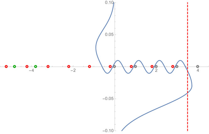
Figure 1: (Color online). Plot of the contour deformation in the complex $t$-plane for the Barnes integral representation Eq.(131) for the hypergeometric function. The straight blue curve is the contour ( $C_{1}$ ) in Eq.(131). The dashed red vertical line is the contour ( $C_{2}$ ) in Eq.(133). The circled crosses correspond to the poles of the various $\Gamma$ functions in the integrand of Eq.(131): the blue ones (at $t=0,1,2,\dots$) are those of $\Gamma(-t)$; the green ones (at $t=-a,-a-1,-a-2,\dots$) are those of $\Gamma(a+t)$; the red ones (at $t=-b,-b-1,-b-2,\dots$) are those of $\Gamma(b+t)$. This plot is for the case $k=1$, $\ell=2$, $s=0$, $\bar{\omega}=-0.1i$, which yields $a=3.9+O(\bar{\omega}^{2})$, $b=-3.1+O(\bar{\omega}^{2})$ and $N=3$.

From the above, we obtain

$$f_{\ell}(r,\omega)=\bar{r}^{s+1}\frac{e^{-i\bar{\omega}\bar{r}}(\bar{r}-1)^{-i\bar{\omega}}}{\sum_{k=-\infty}^{\infty}a_{k}\frac{\Gamma(a)\Gamma(b)}{\Gamma(c)}}\sum_{k=-\infty}^{\infty}a_{k}\cdot(F_{1}(k)+F_{2}(k)).$$ (134)

We note that the integral in $F_{2}$ is exponentially convergent. All that one has to do is completely trivial small-$\bar{\omega}$ expansions of the various coefficients appearing in Eqs.(132) and (133). For that, the small-$\bar{\omega}$ expansions for $\nu$ and for $a_{k}$ of the previous section are required.

VI.3 Cases $\ell=-s=0,1,2$

The results of the previous subsection are valid for any values of the spin $s$ (except for, obviously, Eq.(130)) and multipole number $\ell\geq|s|$. In this subsection we use those results to give the small-$\bar{\omega}$ expansions for the ingoing RW solutions specifically for the modes $\ell=-s=0$, $1$ and $2$, as these are the modes that we will use in the next section in order to calculate the Schwarzschild black hole response to a specific perturbation.

Specifically, for $\ell=s=0$ we have, for general $r$,

$$f_{\ell}(r,-i\sigma)=\bar{r}+\bar{r}\left\{-\log\left(\bar{r}-1\right)-1+\int_{-\infty}^{\infty}dv\frac{(\bar{r}-1)^{\frac{1}{2}+iv}\text{sech}(\pi v)}{1+2iv}\right\}\bar{\sigma}+$$

$$\frac{\bar{r}}{6}\left\{\bar{r}^{2}+8\bar{r}-6+3\log\left(\bar{r}-1\right)\left(\log\left(\bar{r}-1\right)+2\right)-\right.$$

$$\left.\int_{-\infty}^{\infty}dv\frac{(\bar{r}-1)^{\frac{1}{2}+iv}\text{sech}(\pi v)}{(4v^{2}-8iv-3)}\left(21-3\bar{r}-6i\bar{r}v+10iv+\frac{24}{1+2iv}-6(3+2iv)\log\left(\bar{r}-1\right)\right)\right\}\bar{\sigma}^{2}+o\left(\bar{\sigma}^{2}\right).$$ (135)

For $\ell=-s=1$ we have, for general $r$,

$$f_{\ell}(r,-i\sigma)=\bar{r}^{2}-\left\{\frac{\bar{r}}{2^{4}}\left(3-2\bar{r}+\bar{r}\log\left(\bar{r}-1\right)\right)+\frac{1}{\pi}\int_{-\infty}^{\infty}dv\left(\bar{r}-1\right)^{\tfrac{5}{2}+iv}\Gamma\left(-iv-\tfrac{5}{2}\right)\Gamma\left(iv+\tfrac{1}{2}\right)\right\}\bar{\sigma}+$$

$$\bigg{\{}20-168\bar{r}+144\bar{r}^{2}+16\bar{r}^{3}+3\bar{r}^{4}+15\bar{r}\log\left(\bar{r}-1\right)\left(6-4\bar{r}+\bar{r}\log\left(\bar{r}-1\right)\right)+$$

$$\left.\frac{1}{4}\int_{-\infty}^{\infty}dv\frac{(\bar{r}-1)^{\frac{5}{2}+iv}\text{sech}(\pi v)\Gamma\left(iv+\tfrac{1}{2}\right)}{\Gamma\left(iv+\tfrac{9}{2}\right)}\left(809-15\bar{r}(1+2iv)-60(7+2iv)\log\left(\bar{r}-1\right)+\right.\right.$$

$$\left.\left.154iv+\frac{720}{2iv+1}+\frac{480}{2iv+3}+\frac{240}{2iv+5}\right)\right\}\frac{\bar{\sigma}^{2}}{30}+o\left(\bar{\sigma}^{2}\right).$$ (136)

For $\ell=-s=2$ we have, for general $r$,

$$f_{\ell}(r,-i\sigma)=\bar{r}^{3}$$

$$-\left\{\frac{1}{6}\left(6\bar{r}^{3}\log\left(\bar{r}-1\right)-19\bar{r}^{3}+30\bar{r}^{2}-15\bar{r}+10\right)+\frac{12}{\pi\bar{r}}\int_{-\infty}^{\infty}dv\left(\bar{r}-1\right)^{\frac{9}{2}+iv}\Gamma\left(-\tfrac{9}{2}-iv\right)\Gamma\left(\tfrac{1}{2}+iv\right)\right\}\bar{\sigma}+$$

$$\left\{\frac{1}{5040\bar{r}}\left[840\bar{r}\log\left(\bar{r}-1\right)\left(3\bar{r}^{3}\log\left(\bar{r}-1\right)-19\bar{r}^{3}+30\bar{r}^{2}-15\bar{r}+10\right)+\right.\right.$$

$$\left.\left.360\bar{r}^{6}+1728\bar{r}^{5}+40385\bar{r}^{4}-67020\bar{r}^{3}+49470\bar{r}^{2}-397760\bar{r}+24860\right]\right.$$

$$\left.+\frac{1}{35\pi\bar{r}}\int_{-\infty}^{\infty}dv\frac{(\bar{r}-1)^{\frac{9}{2}+iv}\Gamma\left(iv+\frac{1}{2}\right)}{\Gamma\left(iv+\frac{13}{2}\right)}\left[175\pi(\bar{r}-1)(13+2iv)\text{sech}(\pi v)+\right.\right.$$

$$\left.\Gamma\left(-\tfrac{9}{2}-iv\right)\Gamma\left(\tfrac{13}{2}+iv\right)\left(420\bar{r}+420\log\left(\bar{r}-1\right)+420\psi\left(iv+\tfrac{1}{2}\right)-420\psi\left(iv+\tfrac{11}{2}\right)-1019\right)\right]\Bigg{\}}\bar{\sigma}^{2}+o\left(\bar{\sigma}^{2}\right),$$ (137)

where $\psi$ is the digamma function.

VII Late-time Tail

In this section we illustrate how one can apply the small-frequency expansions of the previous sections to obtain physically-relevant results: the late-time behaviour to high order of the black hole response, at an arbitrary point, to a field perturbation of arbitrary integer spin. Before we do that in Sec.VII.2, we first derive the late-time tail of the Green function in the next subsection.

VII.1 Late-time Tail of the Green Function

The late-time behaviour of the RW Green function is, via Eq.(17), given by that of its $\ell$-modes ${}_{s}G^{\text{ret}}_{\ell}$. In its turn, the late-time behaviour of ${}_{s}G^{\text{ret}}_{\ell}$ is dominated by the BC $\ell$-modes ${}_{s}G_{\ell}^{BC}$ in Eq.(19). Finally, it follows from the latter equation that ${}_{s}G_{\ell}^{BC}$ at late times is given by the small-frequency behaviour of $\delta{}_{s}G_{\ell}$. We now give more detailed expressions for these expansions.

The radius-independent part of the BC integrand in the BPT case is given in general (except for $\ell=s=0$) in Eq.(116), and specifically in Eqs.(122)–(124) for the lower modes. Let us generically write its small-frequency expansion as:

$$\frac{q^{T}}{\left|W^{T}\right|^{2}}=v_{0}\bar{\sigma}^{2\ell+1}+v_{1}\bar{\sigma}^{2\ell+2}+\left(v_{2a}+v_{2b}\ln\bar{\sigma}\right)\bar{\sigma}^{2\ell+3}+o(\bar{\sigma}^{2\ell+3}),$$ (138)

where the $\bar{\sigma}$-independent constant coefficients $v_{0}$, $v_{1}$ and $v_{2a/b}$ are readily readable from the mentioned equations. In order to obtain the corresponding RW quantity, we can trivially use Eq.(46). We write the small-frequency expansion of the proportionality constant in Eq.(46) as

$$\mathcal{C}=\mathcal{C}_{0}+\mathcal{C}_{1}\bar{\sigma}+\mathcal{C}_{2}\bar{\sigma}^{2}+O(\bar{\sigma}^{3}),$$ (139)

where the $\bar{\sigma}$-independent constant coefficients $\mathcal{C}_{0/1/2}$ can be read off from from Eqs.(47) and (48).

The radius-dependent part of the BC integrand in the RW case is given in general in Eq.(134); all that one has to do is a trivial small-$\bar{\omega}$ expansion of the summand in Eq.(132) and the integrand in Eq.(133) (with the use of Eqs.(90) and (92) in general, and specifically Eq.(99) for the lower modes). Again, let us write the small-frequency expansion of the ingoing RW solution as

$$f_{\ell}(r,-i\sigma)=f_{\ell 0}(r)+f_{\ell 1}(r)\bar{\sigma}+f_{\ell 2}(r)\bar{\sigma}^{2}+O(\bar{\sigma}^{3}),$$ (140)

where the $\bar{\sigma}$-independent (but radius-dependent) coefficients $f_{\ell,0/1/2}$ can be readily obtained in the manner just indicated.

The analytic small-frequency expansions of the radius-independent (Eq.(138) times Eq.(139)) and radius-dependent (Eq.(140) evaluated at $r$ times the same expression but evaluated at $r^{\prime}$) parts of the BC integrand in the RW case are then to be put together in Eq.(21) and integrated as per Eq.(19). The result, for late times is, straight-forwardly,

$${}_{s}G_{\ell}^{BC}=-\frac{(2\ell+2)!}{4\pi M^{2}}\Bigg{\{}\mathcal{C}_{0}v_{0}f_{00}(r,r^{\prime})+(2\ell+3)\bigg{[}\mathcal{C}_{0}v_{0}f_{01}(r,r^{\prime})+\left(\mathcal{C}_{0}v_{1}+\mathcal{C}_{1}v_{0}\right)f_{00}(r,r^{\prime})\bigg{]}{\bar{t}}^{-1}+$$ (141)

$$2(\ell+2)(2\ell+3)\bigg{[}\mathcal{C}_{0}v_{0}f_{012}(r,r^{\prime})+\left(v_{0}\mathcal{C}_{1}+\mathcal{C}_{0}v_{1}\right)f_{01}(r,r^{\prime})+$$

$$\left(\mathcal{C}_{0}v_{2b}\left(\psi(2\ell+5)-\ln\bar{t}\right)+\mathcal{C}_{0}v_{2a}+v_{0}\mathcal{C}_{2}+\mathcal{C}_{1}v_{1}\right)f_{00}(r,r^{\prime})\bigg{]}{\bar{t}}^{-2}\Bigg{\}}{\bar{t}}^{-2\ell-3}+o\left({\bar{t}}^{-2\ell-5}\right),$$

where

$$f_{00}(r,r^{\prime})\equiv f_{\ell 0}(r)f_{\ell 0}(r^{\prime}),\quad f_{01}(r,r^{\prime})\equiv f_{\ell 0}(r)f_{\ell 1}(r^{\prime})+f_{\ell 0}(r^{\prime})f_{\ell 1}(r),$$ (142)

$$f_{012}(r,r^{\prime})\equiv f_{\ell 0}(r)f_{\ell 2}(r^{\prime})+f_{\ell 0}(r^{\prime})f_{\ell 2}(r)+f_{\ell 1}(r)f_{\ell 1}(r^{\prime}).$$

Here we are using the dimensionless time $\bar{t}\equiv t/(2M)$. The leading-order behaviour at late times is, therefore, ${}_{s}G_{\ell}^{BC}\sim t^{-2\ell-3}$ for all integer spins. We also note that the logarithmic behaviour in Eq.(116) for $q^{T}/|W^{T}|^{2}$ for small frequencies led to the appearance of a logarithmic behaviour in ${}_{s}G_{\ell}^{BC}$ as $t^{-2\ell-5}\ln t$. The late-time behaviour of the GF of the $4$-dimensional RW equation is then obtained by replacing ${}_{s}G^{\text{ret}}_{\ell}$ in Eq.(17) by the expansion in Eq.(141).

A similar analysis can be done for the BPT GF, but using the corresponding equations instead: (37) and (35). The radius-independent part of the integrand, $q^{T}/|W^{T}|^{2}$, we have already given for the BPT case. The radius-dependent part can be obtained from the expansions Eq.(140) of the ingoing RW solutions via the Chandrasekhar transformation of Eq.(39). The late-time behaviour of the $\ell$-modes of the BPT GF is of the same leading order as that in the RW case (i.e., $t^{-2\ell-3}$) and the logarithmic term also generally appears at the same order as in the RW case (i.e., $t^{-2\ell-5}\ln t$).

VII.2 Late-time Tail of an Initial Perturbation

We shall now give a particular application of our late-time results for the GF. Let us here consider an initial field perturbation given by $u_{\ell}^{ic}(r^{\prime}_{*})\equiv u_{\ell}(r^{\prime}_{*},t^{\prime}=0)$ for the $\ell$-multipole of the field and $\dot{u}_{\ell}^{ic}(r^{\prime}_{*})\equiv\partial_{t}u_{\ell}(r^{\prime}_{*},t^{\prime}=0)$ for the $\ell$-multipole of the time derivative of the field. Then the response of a Schwarzschild black hole is given by

$$u_{\ell}(r_{*},t)=\int_{-\infty}^{\infty}dr^{\prime}_{*}\left[{}_{s}G^{\text{ret}}_{\ell}(r,r^{\prime};t)\dot{u}_{\ell}^{ic}(r^{\prime}_{*})+u_{\ell}^{ic}(r^{\prime}_{*})\frac{\partial}{\partial t}{}_{s}G^{\text{ret}}_{\ell}(r,r^{\prime};t)\right],$$ (143)

where $G^{ret}_{\ell}(r,r^{\prime};t)$ is the $\ell$-multipole of the retarded GF of the wave equation satisfied by the field. In this section we will take the RW equation as the wave equation. The late-time asymptotics of the perturbation $u_{\ell}$ are given by replacing ${}_{s}G^{\text{ret}}_{\ell}$ by ${}_{s}G_{\ell}^{BC}$ in Eq.(143) and approximating ${}_{s}G_{\ell}^{BC}$ by performing a small-frequency expansion of $\delta{}_{s}G_{\ell}$ in Eq.(19).

As in Casals and Ottewill (2012b), let us consider the following initial perturbation for general spin

$$u_{\ell}^{ic}(r_{*})=\frac{1}{M}\text{exp}\left(\frac{-\left(r_{*}-x_{0}\right)^{2}}{2M^{2}}\right),\quad\dot{u}_{\ell}^{ic}(r_{*})=-\frac{\left(r_{*}-x_{0}\right)}{M^{2}}u_{\ell}^{ic}(r_{*}),$$ (144)

with $x_{0}\equiv r_{*}(10M)$.

In Figs.2–6 we plot the time evolution via the RW equation of a spin-$s$ field for various multipole numbers $\ell$ using the initial data Eq.(144), similarly to Casals and Ottewill (2012b) where we only presented the case $s=0$, $\ell=1$. We calculate the time evolution numerically up to $T=3000M$, where $T\equiv t-2x_{0}$, and we compare it with late-time asymptotics. The numerical solution is obtained using the code in Wardell for the $(1+1)$-dimensional differential equation which results from the 4-d RW equation after factorizing out the angle dependence of the solution via scalar spherical harmonics. We obtain the late-time asymptotics, up to four leading orders, from the results of the previous section. In order to obtain the small-frequency expansion of $\delta{}_{s}G_{\ell}$ via Eq.(21), we need the small-frequency expansion of $q/|W|^{2}$ and of the ‘in’ radial solution $f_{\ell}$. We now give the specific expansions of the perturbation response for different spins $s$ and $\ell$ modes.

We found the late-time asymptotics for the case $s=0$ and $\ell=0$ using Eq.(VI.3) for the radial solution and Eq.(122) for $q/|W|^{2}$ ; for $\ell=1,2$ we merely inserted the corresponding value of $\ell$ into Eq.(V.4). The results are the following (the approximation sign is due to the fact that we have rounded up the coefficients to seven significant figures):

$$u_{\ell}^{BC}\approx\frac{20.02467}{\bar{T}^{3}}-\frac{269.1100}{\bar{T}^{4}}+\frac{-881.0855\ln\left(\bar{T}\right)+7561.913}{\bar{T}^{5}}+o\left(\bar{T}^{-5}\right),\quad s=\ell=0,$$ (145)

$$u_{\ell}^{BC}\approx-\frac{1144.318}{\bar{T}^{5}}+\frac{52385.24}{\bar{T}^{6}}+\frac{43484.10\ln\left(\bar{T}\right)-1746947}{\bar{T}^{7}}+o\left(\bar{T}^{-7}\right),\quad s=0,\ \ell=1,$$ (146)

$$u_{\ell}^{BC}\approx\frac{42634.22}{\bar{T}^{7}}-\frac{3114525}{\bar{T}^{8}}+\frac{-1796322\ln\left(\bar{T}\right)+146090980}{\bar{T}^{9}}+o\left(\bar{T}^{-9}\right),\quad s=0,\ \ell=2.$$ (147)

Figs.2–4 show excellent agreement at late times between the numerical solution of the RW equation for $s=0$ and $\ell=0,1,2$ and the late-time asymptotics of Eqs.(145)–(147).

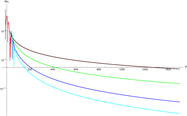
Figure 2: Scalar field $Mu_{\ell}$ at $r_{*}=x_{0}$ as a function of time $T/M$ for the initial data Eq.(144) with $x_{0}=r_{*}(10M)$ and $s=\ell=0$ (i.e., similar to Fig.1 in Casals and Ottewill (2012b) and with the same initial data but here it is for $s=\ell=0$). Red curve: numerical solution. Dashed black curve (overlapping with red curve): late-time expression given by Eq.(145) (which comes from Eqs.(122) together with the small-$\bar{\sigma}$ results in Sec.VI for the radial function). Green curve: numerical solution minus the leading order (i.e., $O(\bar{T}^{-3})$) in the late-time expression. Solid blue curve: numerical solution minus the two leading orders (i.e., $O(\bar{T}^{-3})$ and $O(\bar{T}^{-4})$) in the late-time expression. Solid cyan curve: numerical solution minus the four leading orders (i.e., $O(\bar{T}^{-3})$, $O(\bar{T}^{-4})$, $O(\bar{T}^{-5}\ln(\bar{T}))$ and $O((\bar{T})^{-5})$) in the late-time expression.

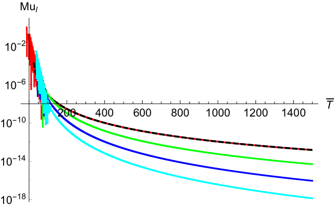
Figure 3: Similar to Fig.2 but here it is for $s=0$, $\ell=1$ (the orders subtracted from the numerical solution are the corresponding leading order, next-to-leading order and four leading orders for this case). The late-time expression is given by Eq.(146).

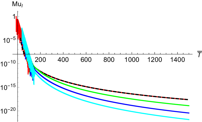
Figure 4: Similar to Fig.2 but here it is for $s=0$, $\ell=2$ (the orders subtracted from the numerical solution are the corresponding leading order, next-to-leading order and four leading orders for this case).

The late-time asymptotics for the RW cases $|s|=\ell=1$ and $2$ are obtained similarly to those above for $s=0$: we used Eqs.(VI.3) and (VI.3) for the small-frequency expansions of the radial solution and Eqs.(123) and (124) for that of $q^{T}/|W^{T}|^{2}$, which is then simply converted to RW version with the use of Eqs.(44) and (153). The final results for the late-time perturbation are the following:

$$u_{\ell}^{BC}\approx-\frac{1338.214}{\bar{T}^{5}}+\frac{59157.01}{\bar{T}^{6}}-\frac{1970216-62896.05\ln\left(\bar{T}\right)}{\bar{T}^{7}}+o\left(\bar{T}^{-7}\right),\quad|s|=\ell=1,$$ (148)

and

$$u_{\ell}^{BC}\approx\frac{60748.13}{\bar{T}^{7}}-\frac{4318418}{\bar{T}^{8}}+\frac{(198106997-3466693\ln\left(\bar{T}\right)}{\bar{T}^{9}}+o\left(\bar{T}^{-9}\right),\quad|s|=\ell=2.$$ (149)

Figs.5–6 show excellent agreement at late times between the numerical solution of the RW equation for $|s|=\ell=1,2$ and the late-time asymptotics of Eqs.(148)–(149).

The above examples illustrate the appearance of a higher-order logarithmic behaviour of a perturbation response, appearing after Price’s well-known power-law tail Price (1972a, b). We note that, as already pointed out in Sec.V.4, this logarithmic behaviour appears at third leading order at late times. It appears at third leading order, not at second leading order as one might have naively expected from the fact that the logarithmic behaviour at small frequency appears at the second leading order both in the BC strength $q^{T}$ and in the Wronskian. This is due to there being delicate cancellations between certain terms of $q^{T}$ and the Wronskian, which we have been able to derive using the precise values of the coefficients in the expansions.

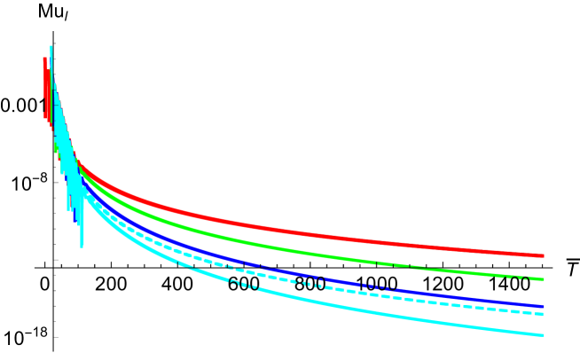
Figure 5: Similar to Fig.2 but here it is the RW solution for $|s|=\ell=1$ (the orders subtracted from the numerical solution are the corresponding leading order, next-to-leading order and four leading orders for this case).

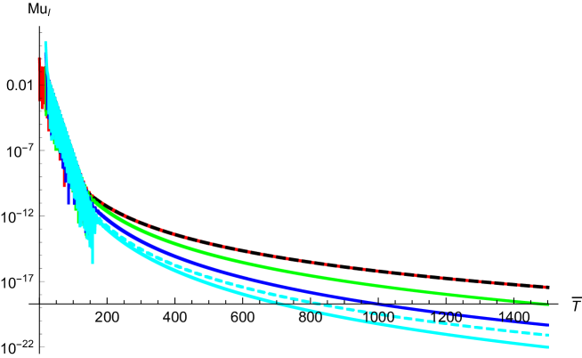
Figure 6: Similar to Fig.2 but here it is the RW solution for $|s|=\ell=2$ (the orders subtracted from the numerical solution are the corresponding leading order, next-to-leading order and four leading orders for this case).

VIII Conclusions

In this paper we have developed the MST formalism for the solutions of the radial Regge-Wheeler and Bardeen-Press-Teukolsky equations, which are obeyed by linear field perturbations of a Schwarzschild black hole space-time. We have derived, for the first time, the MST formalism for the solutions of the RW equation for spin-1 as well as the MST expressions for the branch-cut-relevant quantities for general spin. We have given explicit expansions for small frequency up to the first four leading orders for the various MST quantities for general spin. In principle, the MST series could be expanded to arbitrarily large order in the frequency. The main difficulty in achieving that is the fact that the small-frequency expansion of the renormalized angular momentum parameter $\nu$ that we currently use does not reproduce the numerically-observed behaviour of a sudden appearance of an imaginary part in $\nu$ as the frequency is increased from 0 to larger real values.

We have used our small-frequency expansions in order to obtain the late-time behaviour for arbitrary radius of spin-field perturbations of a Schwarzschild black hole up to the first four leading orders (for a specific multipole-$\ell$). Our results explicitly reveal a new logarithmic behaviour at third order for late times as $t^{-2\ell-5}\ln t$. We note that the appearance of a logarithmic behaviour was already predicted by other works (see, e.g., Ching et al. (1995b, a); Hod (1999, 2009)). However, to the best of our knowledge, the order at which the logarithmic behaviour appears was not correctly predicted anywhere (nor was the calculation of the coefficients for general radius carried out). As we noted at the end of Sec.V.4, there is a delicate cancellation between different logarithmic terms which averts the appearance of a logarithmic behaviour at a lower order; this delicate cancellation is probably hard to predict unless an exact and detailed analysis is carried out such as the one in this paper (see also Smith and Burko (2006), where they find numerical evidence that the logarithmic behaviour does not appear at first nor second leading orders).

We succinctly presented in the Letter Casals and Ottewill (2012b) the final results that we have derived in this paper. We already used some of these results in the calculation of the scalar self-force in Schwarzschild space-time carried out in Casals et al. (2013). The natural extension of our results is the explicit calculation of the small-frequency expansions of the MST quantities for the Teukolsky equation in Kerr space-time, with the corresponding late-time analysis of perturbations of a Kerr black hole. We expect to present the Kerr analysis in the near future, together with its application to a self-force calculation.

Finally, while the calculation of the quasinormal modes has been applied to the modelling of radiation after the inspiral of two black holes via a matching to a numerical relativity solution, to the best of our knowledge, the branch cut has never been taken into account for such purposes. We would expect that the inclusion in the modelling of the branch cut, together with the quasinormal modes, would help match the analytical solution from perturbation theory with the numerical relativity one.

Appendix A Validation of BC results

In this section we compare the small-$\bar{\sigma}$ results presented in this paper with an independent method which we presented in Casals and Ottewill (2013). The latter method is naturally-adapted to a ‘mid-frequency’ regime (which, although valid for all frequencies, is not practical to use in the asymptotic small- or large-frequency regimes). In this appendix we illustrate with plots that there is a region of overlap between the results obtained with the small-$\bar{\sigma}$ method presented here and those obtained with the mid-frequency method of Casals and Ottewill (2013). In Casals and Ottewill (2013) we already presented plots of quantities focused mainly on the $s=\ell=2$ case. Therefore, for variety, here we will focus on the $s=0$ and $\ell=0,1$ cases.

As explained in Casals and Ottewill (2013), the ingoing radial function $f_{\ell}(r,\omega)$ possesses simple poles along the NIA (which are ultimately irrelevant, as they are cancelled out in the Fourier modes of the GF by the corresponding poles in the Wronskian). It is therefore useful to define the following radial function: $\hat{f}_{\ell}(r,\omega)\equiv\sin(-2\pi i\bar{\omega})f_{\ell}(r,\omega)$.

In Figs.7, 8, 9 and 10 we respectively plot the radial function $f_{\ell}$, the BC ‘strength’ $q(\sigma)$, the Wronskian $W$ and the BC mode $\delta{}_{s}G_{\ell}\left(r,r^{\prime},-i\sigma\right)$, all as functions of the frequency $\bar{\sigma}$ along the NIA.

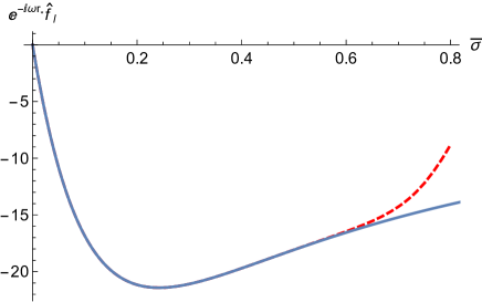
Figure 7: The radial function $e^{-i\omega r_{*}}\hat{f}_{\ell}(r,\omega)$ at $r=10M$ as a function of $\bar{\sigma}$ for $s=0$, $\ell=1$. We calculated the straight blue curve using the so-called Jaffé series (see, e.g., Leaver (1986a); Casals and Ottewill (2013)). and the dashed red curve using the small-frequency asymptotics presented in this paper up to $O(\bar{\sigma}^{15})$ (specifically, using Eq.137 Sasaki and Tagoshi (2003) as in this case we did not need to obtain the coefficients of the expansion analytically via the use of the Barnes integral method).

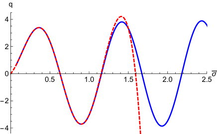
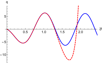
Figure 8: BC ‘strength’ $q(\sigma)$ of Eq.(20) (or, equivalently for $s=0$, $q^{T}(\sigma)$ of Eq.(36)) as a function of $\bar{\sigma}$. In the straight blue curves we calculated $q(\sigma)$ using the mid-frequency method of Casals and Ottewill (2013) (with the radial functions calculated at $r=5M$). In the dashed red curves we calculated $q(\sigma)$ using the small-frequency asymptotics presented in this paper up to $O(\bar{\sigma}^{15})$. (a) For $s=0$, $\ell=0$. (b) For $s=0$, $\ell=1$.

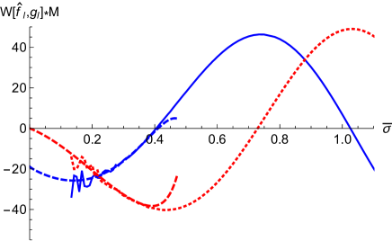
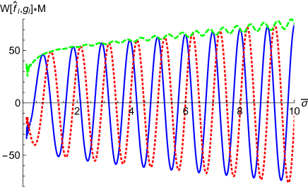
Figure 9: The Wronskian $W\left[\hat{f}_{\ell},g_{\ell}\right]$ as a function of $\bar{\sigma}$ for $s=0$, $\ell=1$. The straight-blue and dotted-red curves respectively correspond to the real and imaginary parts of the Wronskian evaluated using the mid-frequency method of Casals and Ottewill (2013) with the radial functions calculated at at $r=2.8M$; the convergence of the series used in the mid-frequency method becomes slower as the frequency becomes smaller. The dashed blue and red curves respectively correspond to the real and imaginary parts of the Wronskian evaluated using the small-frequency asymptotics presented in this paper up to $O(\bar{\sigma}^{14})$. In figure (b) we plot the mid-frequency to larger values of the frequency so as to show its general form; the green-dashed curve here corresponds to the absolute value of the Wronskian. Cf. Fig.13 Casals and Ottewill (2013) for $s=\ell=2$.

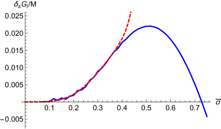
Figure 10: BC mode $\delta{}_{s}G_{\ell}\left(r,r^{\prime},-i\sigma\right)$ of Eq.(21) as a function of $\bar{\sigma}$ at $r=r(r_{*}=0.4M)$, $r^{\prime}=r^{\prime}(r_{*}=0.2M)$ for $s=0$ and $\ell=1$. In the straight blue curve we calculated tbe BC mode using the mid-frequency method of Casals and Ottewill (2013) and in the dashed red curve we calculated it using the small-frequency asymptotics presented in this paper up to $O(\bar{\sigma}^{15})$.

Appendix B Radial Coefficients

In this appendix we use the Chandrasekhar transformation Eq.(38) in order to relate the BPT and RW radial coefficients and Wronskians. Let us first add higher orders to the asymptotics in Eq.(11) of the RW solution:

$$f_{\ell}\sim\begin{cases}\left(1+\alpha_{+}\Delta+\beta_{+}\Delta^{2}\right)e^{-i\omega r_{*}},&r_{*}\to-\infty,\\ A^{in}_{\ell}\left(1+\frac{\alpha_{\infty}}{r}+\frac{\beta_{\infty}}{r^{2}}\right)e^{-i\omega r_{*}}+A^{out}_{\ell}e^{+i\omega r_{*}},&r_{*}\to+\infty,\end{cases}$$ (150)

where $\alpha_{+}$, $\beta_{+}$, $\alpha_{\infty}$ and $\beta_{\infty}$ are coefficients to be determined. By imposing that these asymptotics satisfy the RW equation, we find

$$\alpha_{\infty}=-\frac{i\lambda}{2\omega},\quad\beta_{\infty}=\frac{\lambda(2-\lambda)+4Mi(s^{2}-1)\omega}{8\omega^{2}},$$ (151)

$$\alpha_{+}=\frac{i\left(\lambda+1-s^{2}\right)}{4M^{2}(4M\omega+i)},\quad\beta_{+}=\frac{4-s^{4}-\lambda^{2}+\lambda(2-16iM\omega)+s^{2}(2\lambda+20iM\omega-3)-20iM\omega}{64M^{4}(2M\omega+i)(4M\omega+i)}.$$

We note that $\alpha_{\infty},\alpha_{+},\beta_{\infty},\beta_{+}$ are all real-valued when $\omega$ is purely imaginary.

Using the transformation Eq.(38) it is straight-forward to find the following coefficients of BPT solutions:

$${}_{s}\tilde{R}^{in,inc}_{\ell}=\begin{cases}A^{in}_{\ell},&s=0,\\ \displaystyle-\alpha_{\infty}A^{in}_{\ell}&s=-1,\\ \displaystyle 2\beta_{\infty}A^{in}_{\ell},&s=-2.\end{cases}\quad{}_{s}\tilde{R}^{in,tra}_{\ell}=\begin{cases}\frac{1}{2M},&s=0,\\ \displaystyle\alpha_{+}&s=-1,\\ \displaystyle\frac{2(\alpha_{+}+2M^{2}\beta_{+})}{M},&s=-2.\end{cases}\quad{}_{s}\tilde{R}^{up,tra}_{\ell}=\begin{cases}1,&s=0,\\ \displaystyle 2i\omega&s=-1,\\ \displaystyle-4\omega^{2},&s=-2.\end{cases}$$ (152)

It then immediately follows, using Eqs.(13) and (34), that

$$W^{T}=W\cdot\begin{cases}2M,&s=0,\\ \displaystyle\frac{-\alpha_{\infty}}{\alpha_{+}},&s=-1,\\ \displaystyle\frac{M\beta_{\infty}}{\alpha_{+}+2M^{2}\beta_{+}},&s=-2.\end{cases}$$ (153)

Note that $W^{T}$ is, by definition, independent of the chosen normalization for ${}_{s}R^{in}_{\ell}$ and ${}_{s}R^{up}_{\ell}$.

References

- Regge and Wheeler (1957) T. Regge and J. A. Wheeler, Phys. Rev. 108, 1063 (1957).
- Wheeler (1955) J. A. Wheeler, Phys. Rev. 97, 511 (1955).
- Price (1972a) R. H. Price, Phys. Rev. D5, 2419 (1972a).
- Price (1972b) R. H. Price, Phys. Rev. D5, 2439 (1972b).
- Zerilli (1970a) F. J. Zerilli, Phys. Rev. Lett. 24, 737 (1970a).
- Zerilli (1970b) F. J. Zerilli, Phys. Rev. D 2, 2141 (1970b).
- Ruffini et al. (1972) R. Ruffini, J. Tiomno, and C. Vishveshwara, Lettere Al Nuovo Cimento (1971–1985) 3, 211 (1972).
- Teukolsky (1972) S. A. Teukolsky, Physical Review Letters 29, 1114 (1972).
- Teukolsky (1973) S. A. Teukolsky, Astrophys. J. 185, 635 (1973).
- Bardeen and Press (1973) J. M. Bardeen and W. H. Press, Journal of Mathematical Physics 14, 7 (1973).
- Leaver (1986a) E. W. Leaver, J. Math. Phys. 27, 1238 (1986a).
- Mano et al. (1996a) S. Mano, H. Suzuki, and E. Takasugi, Prog. Theor. Phys. 95, 1079 (1996a).
- Mano et al. (1996b) S. Mano, H. Suzuki, and E. Takasugi, Prog. Theor. Phys. 96, 549 (1996b), arXiv:gr-qc/9605057 .
- Sasaki and Tagoshi (2003) M. Sasaki and H. Tagoshi, Living Rev. Rel. 6, 6 (2003), arXiv:gr-qc/0306120 .
- Poisson et al. (2011) E. Poisson, A. Pound, and I. Vega, Living Rev. Rel. 14, 7 (2011), arXiv:1102.0529 [gr-qc] .
- Hikida et al. (2004) W. Hikida, S. Jhingan, H. Nakano, N. Sago, M. Sasaki, and T. Tanaka, Progress of theoretical physics 111, 821 (2004).
- Hikida et al. (2005) W. Hikida, S. Jhingan, H. Nakano, N. Sago, M. Sasaki, and T. Tanaka, Progress of theoretical physics 113, 283 (2005).
- Casals et al. (2013) M. Casals, S. Dolan, A. C. Ottewill, and B. Wardell, Phys. Rev. D 88, 044022 (2013).
- Bini and Damour (2014a) D. Bini and T. Damour, Physical Review D 89, 064063 (2014a).
- Bini and Damour (2014b) D. Bini and T. Damour, Phys. Rev. D 90, 024039 (2014b).
- Bini and Damour (2014c) D. Bini and T. Damour, Phys. Rev. D 89, 104047 (2014c).
- Shah et al. (2014) A. G. Shah, J. L. Friedman, and B. F. Whiting, Phys. Rev. D 89, 064042 (2014).
- Shah (2014) A. G. Shah, (2014), arXiv:1403.2697 [gr-qc] .
- Delsate et al. (2013) T. Delsate, J. Steinhoff, and S. Chakrabarti, Physical Review Letters (2013).
- Leaver (1986b) E. W. Leaver, Phys. Rev. D 34, 384 (1986b).
- Ching et al. (1995a) E. S. C. Ching, P. T. Leung, W. M. Suen, and K. Young, Phys. Rev. D52, 2118 (1995a), arXiv:gr-qc/9507035 .
- Casals and Ottewill (2013) M. Casals and A. C. Ottewill, Phys.Rev. D87, 064010 (2013), arXiv:1210.0519 [gr-qc] .
- Casals and Ottewill (2012a) M. Casals and A. Ottewill, Phys.Rev. D86, 024021 (2012a), arXiv:1112.2695 [gr-qc] .
- Maassen van den Brink (2000) A. Maassen van den Brink, Phys. Rev. D62, 064009 (2000), arXiv:gr-qc/0001032 .
- Maassen van den Brink (2004) A. Maassen van den Brink, J. Math. Phys. 45, 327 (2004), arXiv:gr-qc/0303095 .
- Casals and Ottewill (2012b) M. Casals and A. Ottewill, Phys. Rev. Lett. 109, 111101 (2012b).
- Zhang et al. (2013) Z. Zhang, E. Berti, and V. Cardoso, Physical Review D 88, 044018 (2013).
- Nakano and Sasaki (2001) H. Nakano and M. Sasaki, Prog.Theor.Phys. 105, 197 (2001), arXiv:gr-qc/0010036 [gr-qc] .
- Chandrasekhar (1983) S. Chandrasekhar, The Mathematical Theory of Black Holes (Oxford University Press, New York, 1983).
- Leung et al. (2003) P. T. Leung, A. Maassen van den Brink, K. W. Mak, and K. Young, (2003), arXiv:gr-qc/0307024 .
- Goldberg et al. (1967) J. Goldberg, A. Macfarlane, E. T. Newman, F. Rohrlich, and E. Sudarshan, Journal of Mathematical Physics 8, 2155 (1967).
- Newman and Penrose (1966) E. T. Newman and R. Penrose, Journal of Mathematical Physics 7, 863 (1966).
- Chandrasekhar (1975) S. Chandrasekhar, Proceedings of the Royal Society of London. A. Mathematical and Physical Sciences 343, 289 (1975).
- Jensen et al. (1991) B. P. Jensen, J. G. McLaughlin, and A. C. Ottewill, Physical Review D 43, 4142 (1991).
- (40) DLMF, “NIST Digital Library of Mathematical Functions,” http://dlmf.nist.gov/, Release 1.0.5 of 2012-10-01, online companion to Olver et al. (2010).
- Gradshteyn and Ryzhik (2007) I. Gradshteyn and I. Ryzhik, Table of Integrals, Series, and Products (Academic Press, 2007).
- Erdelyi et al. (1953) A. Erdelyi, W. Magnus, F. Oberhettinger, and F. Tricomi, Higher Transcendental Functions (McGraw-Hill, New York, 1953).
- Teukolsky and Press (1974) S. A. Teukolsky and W. Press, The Astrophysical Journal 193, 443 (1974).
- Casals (2004) M. Casals, Electromagnetic Quantum Field Theory on Kerr-Newman Black Holes, Ph.D. thesis, University College Dublin (2004), arXiv:0802.1885 .
- Page (1976) D. N. Page, Phys. Rev. D 13, 198 (1976).
- (46) http://dlmf.nist.gov/.
- Jensen et al. (1995) B. P. Jensen, J. G. McLaughlin, and A. C. Ottewill, Phys. Rev. D 51, 5676 (1995).
- Wardell et al. (2014) B. Wardell, C. R. Galley, A. Zenginoğlu, M. Casals, S. R. Dolan, and A. C. Ottewill, Phys. Rev. D 89, 084021 (2014).
- (49) B. Wardell, https://github.com/barrywardell/scalarwave1d.
- Ching et al. (1995b) E. S. C. Ching, P. T. Leung, W. M. Suen, and K. Young, Phys. Rev. Lett. 74, 2414 (1995b), arXiv:gr-qc/9410044 .
- Hod (1999) S. Hod, Phys.Rev. D60, 104053 (1999), arXiv:gr-qc/9907044 [gr-qc] .
- Hod (2009) S. Hod, Class.Quant.Grav. 26, 028001 (2009), arXiv:0902.0237 [gr-qc] .
- Smith and Burko (2006) A. Z. Smith and L. M. Burko, Phys.Rev. D74, 028501 (2006), arXiv:gr-qc/0510008 [gr-qc] .
- Olver et al. (2010) F. W. J. Olver, D. W. Lozier, R. F. Boisvert, and C. W. Clark, eds., NIST Handbook of Mathematical Functions (Cambridge University Press, New York, NY, 2010) print companion to DLMF .