New expansion rate measurements of the Crab Nebula in radio and optical

Abstract

We present new radio measurements of the expansion rate of the Crab nebula’s synchrotron nebula over a $\sim$30-yr period. We find a convergence date for the radio synchrotron nebula of ce $1255\pm 27$. We also re-evaluated the expansion rate of the optical line emitting filaments, and we show that the traditional estimates of their convergence dates are slightly biased. Using an un-biased Bayesian analysis, we find a convergence date for the filaments of ce $1091\pm 34$ ($\sim 40$ yr earlier than previous estimates). Our results show that both the synchrotron nebula and the optical line-emitting filaments have been accelerated since the explosion in ce 1054, but that the synchrotron nebula has been relatively strongly accelerated, while the optical filaments have been only slightly accelerated. The finding that the synchrotron emission expands more rapidly than the filaments supports the picture that the latter are the result of the Rayleigh-Taylor instability at the interface between the pulsar-wind nebula and the surrounding freely-expanding supernova ejecta, and rules out models where the pulsar wind bubble is interacting directly with the pre-supernova wind of the Crab’s progenitor.

1 Introduction

The Crab Nebula is one of the most intensely studied objects in astrophysics, yet it retains the power to surprise us (see Bühler & Blandford, 2014; Hester, 2008, for recent reviews). It is the remnant of a supernova explosion in the year ce 1054, which was witnessed by Chinese and other astronomers (Stephenson & Green, 2003). The presently visible nebula is bright at all observable wavelengths, and contains one of the first known pulsars, PSR B0531+21. The pulsar’s spin frequency is 30 Hz, and it is slowing down at a rate of $-3.78\times 10^{-10}$ Hz s^-1 (Lyne et al., 2015). The Crab Nebula is the prototype of a pulsar-powered nebula, commonly known as a pulsar wind nebula (PWN), where the rotational energy lost by the spinning down of the pulsar powers the nebula. The energy input from the pulsar, which emerges in the form of a wind of magnetic field and relativistic particles, inflates a large bubble of relativistic fluid, which emits synchrotron radiation. The synchrotron-emitting fluid expands into the supernova ejecta, with which it interacts both dynamically and by photoionizing them. The synchrotron-emitting bubble and the optical-line emitting filaments of photoionized thermal gas constitute the bulk of the presently visible nebula.

The Crab has recently been discovered to produce substantial flares at gamma-ray wavelengths, where the emission at energies $>100$ MeV increases by more than a factor of two on timescales of days (e.g. Bühler & Blandford, 2014, and references therein). The origin of these flares is not yet well understood. Since they are poorly localized in gamma-rays, we obtained radio observations of the Crab following a gamma-ray flare in 2012 August to look for a radio counterpart. Our initial results are reported in Bietenholz et al. (2015): we did not find any such radio counterparts. We did, however, obtain high-quality radio images of the Crab. In the present paper, we use those radio images (from epoch 2012), and compare them to earlier radio images to more accurately determine the expansion rate of the synchrotron nebula.

The PWN inflated by the pulsar continues to expand, and the Crab nebula is young and close enough that the expansion has been directly observed at different wavelengths. In fact, not only is the Crab expanding, it has been accelerated since the ce 1054 explosion. Several authors have measured the proper motions of the optical filaments over the years (e.g., Duncan, 1939; Woltjer, 1958; Trimble, 1968; Wyckoff & Murray, 1977; Nugent, 1998), and from these calculated a convergence date, which is the date on which the filaments would have been closest together if their present positions and proper motions are extrapolated backwards in time. This convergence date is later than the known explosion date of ce 1054, indicating an accelerated expansion.

The expansion rate of the nebula was also determined in the radio by Bietenholz et al. (1991), who used VLA observations taken between 1981 and 1988. This radio measurement gave a determination of the expansion speed of the pulsar wind bubble (as opposed to that of the optical line-emitting filaments), and showed that the former was expanding at a rate slightly higher than, but within the uncertainties, of that observed for the filaments.

In the canonical picture of the Crab, such acceleration is in fact expected, because the PWN is expanding into the supernova ejecta, which themselves are still freely expanding. Since the ejecta expand with velocity proportional to the radius, as the PWN expands into the ejecta, it must move ever faster to overtake them, so as long as there is continued energy input from the pulsar and the PWN remains within the freely-expanding ejecta, the PWN bubble is expected to accelerate (see, e.g. Reynolds & Chevalier, 1984; Chevalier, 1984).

If SN 1054 was a normal supernova, then it would be expected to have released about $10^{51}$ erg of energy. The presently visible Crab nebula, however, contains at most 10% of this energy. It is mostly thought that the remainder of the expected $10^{51}$ erg resides in freely expanding ejecta, outside the presently visible nebula. There has as yet been no convincing direct detection of this “outer shell” of ejecta, despite the fact that it is predicted to be substantially ionized by the flux from the PWN (Lundqvist et al., 1986; Wang et al., 2013).

Nonetheless, circumstantial evidence does suggest that the presently visible nebula is confined by the unseen massive ejecta. In this picture, the optically-bright filaments are the product of a Rayleigh-Taylor instability between the low-density but high-pressure synchrotron-emitting fluid and the massive ejecta. Hester (2008) gives a summary of the arguments for this interpretation.

We note here, however, that there is an alternate interpretation, which is that SN 1054 was a low-energy electron-capture event, with only a small ejected mass, and that the presently visible filaments are the result of the PWN interacting with the circumstellar material (Smith, 2013; Tominaga et al., 2013; Moriya et al., 2014). The progenitor in this case is expected to have been a super-asymptotic giant branch star, in other words one at the upper end of the mass range of the asymptotic giant branch, with a mass of around 8 to 10 M$\odot$, although the mass is not well constrained (see Moriya et al., 2014, and references therein). Such progenitors are expected to produce slow, dense winds before the SN explosion.

If the Crab PWN is currently expanding into the freely expanding SN ejecta, then it should, as mentioned above, be the case that the synchrotron bubble is expanding more rapidly than the optical filaments. The measurements of Bietenholz et al. (1991) already suggested that this might be the case, but a better measurement of the expansion of the synchrotron bubble is required to be sure. Although the synchrotron emission is visible in the optical and even in the X-ray, such a measurement is most easily done in the radio where the synchrotron bubble is most clearly visible. We therefore undertook a new and more accurate determination of the expansion rate of the Crab’s PWN using radio images, as well as a re-evaluation of the expansion rate of the optical line-emitting filaments determined from proper motion measurements. The radio and optical data allow us to measure the expansion rate of two different components of the nebula, namely the low-density but high-pressure PWN and the massive line-emitting filaments, respectively.

2 Observations and data reduction

2.1 VLA observations

For the purposes of measuring the expansion rate of the Crab Nebula, we assemble a collection of 5-GHz images taken between 1981 and 2012. Images made from data taken at a specific time, and thus only using a single VLA array configuration would be best-suited for determining the expansion. We concentrate therefore on using images made only from B-configuration data, which was used for the observations between 1998 and 2012. However, due to various reasons, for some of the earlier epochs we use images made from combinations of several configurations, spatially filtered so as to approximate the B-configuration-only images. We will note these epochs below.

Using observations made only in a single VLA array configuration is the equivalent of applying a spatial filter to the images, limiting both the highest spatial frequency (highest resolution) and the lowest one (largest recoverable size). In particular, for the B-array at 5-GHz, the resolution is limited to $\sim 1\aas@@fstack{\prime\prime}2$ and the largest recoverable structure is $\sim$30″. Although the range of spatial frequencies sampled is similar in all our epochs it will not be identical due to slightly different observing frequencies, different observing hour angles and the occasional failure of an antenna. In order to unify our images as much as possible, we further spatially filter our images using a Gaussian kernel. First, we use a spatial low-pass filter to reduce the effective resolution to 2$\aas@@fstack{\prime\prime}$0 $\times$ 1$\aas@@fstack{\prime\prime}$8 at p.a. 80^∘, and secondly a high-pass filter with FWHM of 20″ to exclude poorly sampled large-scale structure.

As already mentioned, we use the 2012 radio observations described in Bietenholz et al. (2015). We give here only a brief description of the observations: there were two sessions of VLA observations on 2012 August 20 and 26, spaced 6 days apart (observing code 12A-486). We used a bandwidth 2048 MHz around a central frequency of 5567 MHz, with a total of 5 hours per session. The array was in the B configuration, resulting in native resolutions of $\sim$1″ FWHM, but as mentioned we low-pass filtered them to reduce the effective resolution to 2$\aas@@fstack{\prime\prime}$0 $\times$ 1$\aas@@fstack{\prime\prime}$8 for our expansion measurement.

We also used data from 2000 Feb. 11 and 2001 Apr. 17, described in Bietenholz et al. (2004). These observations were taken with centre frequencies of 4.885 and 4.625 GHz. Both frequencies were combined for imaging. We further used data from 1998 August 8, which is described in Bietenholz et al. (2001), and which was taken with the same centre frequencies.

We further used data taken between 1987 May to 1988 March, again taken at 4.885 and 4.625 GHz and described in Bietenholz & Kronberg (1990), Bietenholz & Kronberg (1991), Bietenholz et al. (1991) and Bietenholz & Kronberg (1992). For these epochs, the calibrated visibility data were no longer available, and we worked with the deconvolved images, which were made with the combined data from the B, CD and D configurations using maximum entropy deconvolution. We again high-pass filter them with a Gaussian of FWHM 20″. This filtering will remove almost all of the information contributed by the D array, and some of that contributed by the C-array. We take as the effective date of this image therefore a weighted average of those of the B and C configurations only, with the B configuration given double the weight of the C configuration. Since all three configurations were observed within one year the effective date is not overly sensitive to variations in this weighting and our results below do not depend on it.

Finally, we also used data from B-configuration taken on 1982 Oct. 16. Since the signal-to-noise ratio of the B-configuration data alone was low, we added some data from the C configuration, taken on 1981 Nov. 29. Both sets of observations were at 4.9 GHz and had a bandwidth of 12.5 MHz. These observations are described in Wilson et al. (1985) and Bietenholz et al. (1991). We re-reduced the archival visibility data, combined the data from both configurations, and then made an image using CLEAN deconvolution. We apply the same prescription as we used for the 1987 epoch to determine the effective date, of taking a weighted mean of the B and C configuration observing dates, with the B-configuration being given twice the weight, and again high- and low-pass filtered the resulting image as we did the others.

3 Expansion of the synchrotron bubble

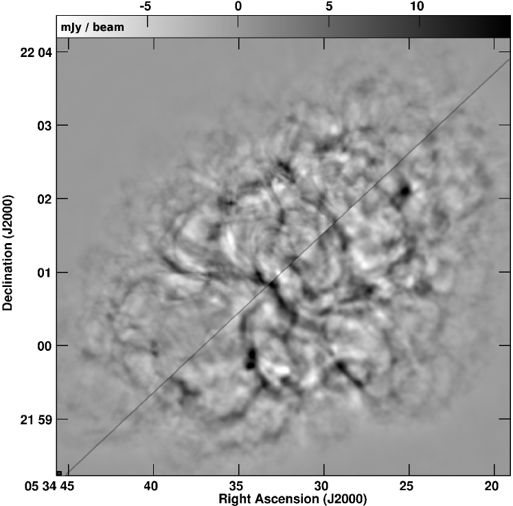
Figure 1: A composite image to illustrate the expansion of the Crab synchrotron nebula. On the top left is the image from 2012 Aug. 26, while on the lower right is the one from 1987 Dec. Both images are 5-GHz VLA radio images, which have been spatially band-limited to show only emission on a limited range of angular scales by convolving to limit the resolution to 2$\aas@@fstack{\prime\prime}$0 $\times$ 1$\aas@@fstack{\prime\prime}$8 at p.a. 80^∘ (FWHM), and high-pass filtering at 20″ (FWHM). Note that the image brightness can have negative as well as positive values because of the high-pass filtering. See text for a fuller description of the data and the processing of the images.

We first measure the expansion rate of the synchrotron bubble using the radio images. To illustrate the expansion we show a composite of the images from 1987 and 2012 in Figure 1. Since there are few sharply-defined features from which the expansion could be directly measured, we use the same approach for determining the expansion as was used in Bietenholz (2006), Bietenholz & Bartel (2008) and Bietenholz et al. (1991), and which was originally developed by Tan & Gull (1985). We repeat a brief description here for the convenience of the reader: rather than determining the proper motion of individual features, we measure the overall expansion by determining the scaling between a pair of images by least-squares. This is accomplished by using the MIRIAD (Sault et al., 1995) task IMDIFF which determines how to make one image most closely resemble another, by calculating unbiased estimators for the scaling in size, $e$, the scaling and the offset in flux density, $A$ and $b$ respectively, and the offsets in RA and decl., $x$ and $y$ respectively, by least squares. Our chief interest is in the expansion factor, $e$, but because of uncertainties in flux calibration, absolute position, and image zero-point offsets caused by missing short spacings and self-calibration and slightly different observing frequencies, all five parameters needed to be determined.

We calculate the expansion from images which were not corrected for the primary beam response. Although the attenuation due to the primary beam is appreciable towards the edge of the nebula at 5 GHz, the uncorrected images are preferred for the expansion calculation because the noise is uniform over the image, which is a desirable property for an algorithm that computes a least-squares fit over the whole image. The use of the uncorrected images should not affect our expansion results because the frequency of observation, and thus the primary beam response, was almost the same at all our epochs and the expansion is small. We re-imaged or re re-sampled all the earlier observations to have the same pixel spacing (0.27″) as the 2012 ones, and also, if required, J2000 coordinates. For each pair of images we compute $e$. To reduce biases, we also repeated the calculation but inverted the order of the images, which causes $1/e$ to be determined. As our final value of $e$ was the average of the two runs (although in all cases the two values of $e$ were consistent to within 0.001). The uncertainty in $e$ is difficult to estimate, we conservatively adopt a value of 0.002 (however, we show below that the scatter in the derived expansion rate suggests a lower uncertainty in $e$ of $\sim 0.0009$). We give our values of $e$ for various pairs of images in Table 2. We define the fractional expansion rate, ${\scriptstyle R}_{\rm exp}$, as the percentage increase in size of the nebula per year. The weighted mean value of ${\scriptstyle R}_{\rm exp}$ over the period of 1982 to 2012, was $0.134\pm 0.005$ % yr^-1 (at the weighted-mean epoch of 1996.6).

From each pair of images, we can also calculate a “convergence date” for the nebula under the assumption of constant-velocity expansion from a single origin. Let $t_{1}$ and $t_{2}$ be the times of two images measured with respect to the time of the explosion, and $\Delta t=t_{2}-t_{1}$. For constant velocity expansion, the value of $e$ between $t_{1}$ and $t_{2}$ is just $(t_{1}+\Delta t)/t_{1}$. From any determination of $e$ we can therefore calculate the value of $t_{1}$ and thus estimate the explosion date. Since the assumption of constant-velocity expansion is well known not to hold for the Crab, we term this date the “convergence date” or convergence year, which in the Crab’s case will be somewhat later than the actual explosion year of ce 1054.

The weighted mean convergence year calculated from our measurements in Table 2 is ce $1243.4\pm 9.3$, with the uncertainty obtained by scaling the input uncertainties to obtain $\chi^{2}_{8}=8$. We also performed a Bayesian calculation to estimate both the convergence year and the true uncertainties in $e$, which as mentioned above were not reliably estimated a priori. We used a uniform prior distribution for the convergence year and a Jeffrey’s prior ($p(\sigma)=1/\sigma$) for the uncertainties in $e$. The posterior distribution of the convergence year was obtained through Markov Chain Monte-Carlo (MCMC) sampling. We obtained a consistent value of ce $1240\pm 12$, with the estimate of the measurement uncertainties in $e$ being 0.0009.

Is there any bias in this determination of the convergence date? We explored the possibility of a bias as follows: we made a copy of a radio image, and expanded it by a factor of exactly 1.02 (i.e. by 2%), then added noise. For the noise, we used Gaussian random noise with the value in each pixel being independent, then convolved with the same CLEAN beam ($2\aas@@fstack{\prime\prime}0\times 1\aas@@fstack{\prime\prime}8$ at p.a. 80^∘) as our images, so that our added noise has same spatial auto-correlation function as that in the real images. We then again used IMDIFF to determine $e$ between this modified copy and the original image. In the absence of any bias, we expect to obtain $e=1.0200$. Over $n=8$ trials we found that the derived average value of $e$ was $1.0205\pm 0.00006$, suggesting that any bias in $e$ is less than 0.00006. We therefore believe that our estimates of $e$ are not significantly biased by the presence of noise in the images.

Does the expansion rate of the Crab change with time? We performed a weighted fit to our measured values of ${\scriptstyle R}_{\rm exp}$, taking the time of each rate measurement as being the midpoint of the two epochs involved. We plot the resulting values of ${\scriptstyle R}_{\rm exp}$ in Figure 2. We found that $\mbox{${\scriptstyle R}_{\rm exp}$}\ =+(5\pm 9)\times 10^{-4}\,t_{1054}-(0.341\pm 0.004)$ % yr^-1. Note that ${\scriptstyle R}_{\rm exp}$ represents the fractional expansion rate, so for constant velocity expansion since ce 1054, $d\mbox{${\scriptstyle R}_{\rm exp}$}/dt$ would be $-1.1\times 10^{-4}$ % yr^-2, and for constant velocity expansion since the convergence date of ce 1250, it would be $-1.8\times 10^{-4}$ % yr^-2. Although our results suggest that ${\scriptstyle R}_{\rm exp}$ is increasing with time, they are well compatible with the expected decrease with time (to within $1\sigma$), and we do not consider the increase with time of ${\scriptstyle R}_{\rm exp}$ significant (see Fig. 2).

Table 1: Images used for the expansion calculation

Date of observations	Julian date
1982 Apr 24a	2445084
1987 Dec 29	2447159 b
1998 Aug 09	2451035
2001 Apr 17	2452016
2012 Aug 26	2456165

^a For this epoch, to increase the signal-to-noise, we combined data taken in the B and C configurations on 1982 Oct. 16 and 1981 Oct. 29, respectively, but used data only at $u$-$v$ distance $>3.3$ K$\lambda$. As the time of these observations, we take a weighted mean, with the B-array, which contributes most of the information, being given double the weight of the C-array. The resulting date is 1982 June 22.
^b For this epoch, we used an image made from B,CD and D configurations, taken on 1987 Nov. 21, 1988 Mar. 14 and 1987 May 26, respectively. Due to the spatial high-pass filtering which will isolate chiefly the information contributed by the B-array we use, as we did for the 1982 epoch, a weighted combination of the B and C configuration dates, with again the B-configuration being given twice the weight. The resulting date is 1987 Oct. 31.

Table 2: Expansion Factors

First Epoch	Second Epoch	Interval	Expansion Factor
		(yr)
1982	1987	5.52	1.007
1982	2001	18.82	1.024
1982	2012	30.18	1.040
1987	1998	10.61	1.015
1987	2001	13.30	1.018
1987	2012	24.66	1.034
1998	2012	14.05	1.019
2001	2012	11.36	1.016

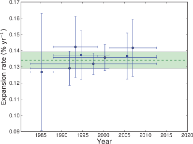
Figure 2: The fractional expansion rate of the Crab Nebula (${\scriptstyle R}_{\rm exp}$), as calculated from pairs of radio images. Each blue point shows a value of the expansion rate derived from one pair of images, with the horizontal bar showing the time interval over which the corresponding rate was calculated, and the vertical one the uncertainty in the derived expansion rate. The green dashed line shows the weighted mean of ${\scriptstyle R}_{\rm exp}$ of $0.134\pm 0.015$ % yr^-1, with the shaded area showing the $1\sigma$ uncertainty on the mean. Near the outside edge of the nebula, ${\scriptstyle R}_{\rm exp}$= 0.135 % yr^-1 corresponds to 2310 km s^-1 ($\theta=3\arcmin,D=2$ kpc).

4 Expansion of the line-emitting filaments

We also re-examined the expansion rate as determined from the proper motions of the line-emitting filaments observed in the optical. We used the proper motion measurements made by Nugent (1998), on the basis of four published high-resolution optical images of the Crab, with the first made in 1939 and the last in 1992 (Baade, 1942; Gingerich, 1977; Parker, 1995; Wainscoat & Kormendy, 1997). The details of the astrometrical reduction and proper motion measurements are given in Nugent (1998).

Previously, the expansion age of the Crab had been determined by extrapolating the present positions backwards using the (presently measured) proper motions (e.g. Nugent, 1998), and taking the convergence date as the time at which the scatter amongst the extrapolated positions was smallest, and the corresponding convergence position as the mean position at that time. This procedure, however, does not properly take into account the uncertainties in the proper motion measurements, and leads to a slightly, but significantly, biased value for the convergence date, as we will illustrate below.

We will assume, like others workers (e.g. Duncan, 1939), that the filaments originated at some particular point in space, namely the convergence point, at some particular time, namely the convergence time, and that they have moved at a constant velocity since then. Since we know in fact that the supernova was in 1054 ce, a convergence date later than 1054 ce implies that the filaments have not in fact been moving at constant speed, but rather have been accelerated since 1054 ce. A more straightforward analysis would be to fix the explosion date at its known value and more directly estimate the amount of acceleration. However, we chose the more indirect method of estimating the convergence date for easier comparison with earlier results. The amount by which the convergence date is later than 1054 ce indicates the amount of acceleration that has taken place.

The bias in the convergence date can easily be illustrated with the following example. Imagine that the Nebula were static, in other words that the convergence date was infinitely far in the past (or the future). The true proper motions would be 0. The measured values would be randomly distributed about zero because of measurement errors. The smallest scatter in the extrapolated positions would be near the present time, since no matter what the random motions, over any length of time they are more likely to move the filaments farther apart than closer together. The date at which the extrapolated position scatter is smallest would therefore be near the present, not infinitely far in the past where the true convergence date is. This bias occurs even if the real proper motions are not zero, in the sense that the date of smallest extrapolated position scatter is always somewhat nearer to the present than the true convergence date.

To take proper account of the errors in both the measured positions and proper motions, we again turn to a Bayesian analysis. We retain the hypothesis that the proper motions are constant in time, and that the filaments all originated at the convergence point in space and at the convergence date in time, and it is the convergence point and date that we wish to estimate. For any given convergence position and date, the present true filament positions and proper motions are functionally related. We treat the measurements of the positions and proper motions as independent, and in our Bayesian analysis we also estimate the true present positions of the filaments. We take the measured proper motions and positions to be Gaussian-distributed about the true values, with standard deviations given by the observational uncertainties.

We take the following prior distributions: uniform with a range of ce 500 to 1500 for the convergence year, Gaussian with $\sigma=200\arcsec$ centred around the present mean position of the filaments for the convergence position, and Gaussian with a with $\sigma=10\arcsec$ centred on the measured positions for the true filament positions. Note that the measured filament positions are very unlikely to be in error by 10″, so our prior distribution should be minimally informative and should therefore have very little effect on the derived posterior distributions.

We again turn to Markov Chain Monte-Carlo to estimate the posterior distributions. We obtain a values for the convergence year of ce $1091\pm 34$, and the convergence position of RA = ${5}^{\mathrm{h}}\;{34}^{\mathrm{m}}\;{33}\aas@@fstack{s}{27}$, decl. = ${22}\degr\;{00}\arcmin\;{42}\aas@@fstack{\prime\prime}{52}$ (J2000).

These convergence year and position estimates are not sensitive to the exact choice of the prior distribution for reasonable choices. We emphasize that our estimate of the convergence year is obtained using exactly the same measurements as Nugent (1998), and the difference between our value and the one Nugent obtained (of ce $1130\pm 16$) is due our Bayesian estimate not being biased towards the present. The bias in Nugent’s (and other earlier values of the convergence year) is not large, although we note that the uncertainty in the convergence year from our Bayesian analysis is larger than that of Nugent’s estimate, which is because our analysis takes the uncertainties in the measured proper motions into account.

5 Discussion

5.1 Expansion and acceleration of the Crab

We found above that the fractional expansion rate of the Crab’s synchrotron bubble, ${\scriptstyle R}_{\rm exp}$, during the period 1982 to 2012 was $0.134\pm 0.005$ % yr^-1, (at mean epoch 1996.6). This value of ${\scriptstyle R}_{\rm exp}$ implies a convergence year of ce $1255\pm 27$. Bietenholz et al. (1991) found ${\scriptstyle R}_{\rm exp}$ for epoch 1987.4 was $0.133\pm 0.016$ and a convergence year of ce $1243\pm 92$ for the whole nebula, which agrees well with our determination (we note that since we used some of the same data as Bietenholz et al., 1991, our ${\scriptstyle R}_{\rm exp}$ estimates are not completely independent from theirs).

It is well known that the Crab Nebula has been accelerated since the explosion (e.g., Trimble, 1968; Wyckoff & Murray, 1977; Bietenholz et al., 1991; Nugent, 1998). The explosion epoch of 1054.5 implies that without acceleration, ${\scriptstyle R}_{\rm exp}$ should be of 0.106 % yr^-1 at epoch 1996.6. Our measured expansion rate for the synchrotron bubble of $0.134\pm 0.005$ % yr^-1 suggests therefore an accelerated expansion and the later convergence date of ce $1255\pm 27$. If we assume a power-law expansion, with $\mbox{$R_{\mathrm{PWN}}$}\propto t^{m}$, then we can calculate that $m=1.264\pm 0.049$. For a spherical pulsar wind nebula expanding into un-shocked supernova ejecta, both theory and simulations predict an approximately power-law expansion, with $m$ in the range of 1.1 to 1.3 (e.g. Chevalier, 1984; van der Swaluw et al., 2001; Bucciantini et al., 2003; Gaensler & Slane, 2006). Our results are therefore consistent with the theoretical expectations, albeit at the higher end of the range of expected values of $m$.

We also determined the convergence year for the optical filaments to be ce $1091\pm 34$, which implies a powerlaw exponent of $m=1.040\pm 0.039$. Since we found $m=1.264\pm 0.049$ for the synchrotron bubble, we can say that the synchrotron bubble is experiencing an acceleration which is stronger than that of the optical filaments by $3.5\sigma$.

Rudie et al. (2008) examined the proper motion of knots in the northern jet, at the northern extremity of the Crab, and found a convergence date of ce $1055\pm 24$. Although this convergence date is earlier than the biased values obtained by other workers for the filaments in the body of the nebula, it is in fact consistent within the combined uncertainties with the unbiased convergence date we obtained for the optical filaments. Rudie et al. (2008) conclude that the jet, unlike the filaments in the body of the nebula, had experienced essentially no acceleration. Since we find a lower acceleration for the bulk of the filaments, the difference between any acceleration experienced by the jet and that experienced by the remainder of the filaments is less clear, and we cannot conclusively say whether or note the jet has experienced less acceleration than the body of the nebula.

The origin of the optical filaments is generally thought to be the following: the pulsar outflow blows a synchrotron-emitting bubble, whose interior has high pressure but low density, into the still freely expanding supernova ejecta. The interface between the pulsar bubble and the ejecta is Rayleigh-Taylor unstable (Chevalier & Gull, 1975; Hester et al., 1996; Hester, 2008). This picture is supported by the fact that the filaments seem to only occur in a thick shell around the exterior of the nebula, but not in the central region (Lawrence et al., 1995; Charlebois et al., 2010). The magnetohydrodynamic simulations of Porth et al. (2014) show that this instability causes “fingers” of ejecta to develop, which then stream downwards into the PWN, while “bubbles” of synchrotron-emitting fluid move outward between them.

In this model, on average the synchrotron nebula would expand more rapidly than the filaments. Our observations show exactly this, and therefore give strong support to the idea that the presently visible optical filaments are largely the result of the Rayleigh-Taylor and other instabilities at the interface between the synchrotron-emitting relativistic fluid from the pulsar and the massive supernova ejecta.

In the alternate scenario of SN 1054 being a low-energy electron-capture event (e.g. Smith, 2013; Tominaga et al., 2013; Moriya et al., 2014), interaction of the supernova shock with the circumstellar medium (CSM) was responsible for the luminosity of SN 1054 as well as for the presently visible filaments, which contain largely swept-up CSM rather than supernova ejecta. The PWN is therefore confined by the dense wind from the super-asymptotic giant branch progenitor of the supernova. In this scenario one would also expect, as we have observed, that the synchrotron nebula expands more rapidly than the filaments. However, our measurement of the strong acceleration of the synchrotron bubble is at odds with this scenario: if this bubble is confined largely by a stellar-wind CSM, expected to have speeds of order 10 km s^-1, or less than 1% of the PWN’s present expansion speed, then one would expect that PWN have been strongly decelerated since the explosion. The opposite seems to be true, as confirmed by our measurement of the relatively strong acceleration of the synchrotron bubble. Our measurement of the acceleration of the synchrotron bubble therefore rule out any scenario where the PWN is interacting with a slowly moving wind.

Recently, Yang & Chevalier (2015) suggested a modified version of the canonical scenario above, where the Crab was indeed the result of a low-energy ($\sim 10^{50}$ erg) supernova. However, although the energy (and mass) of the ejecta is lower than those of a supernova of normal energy ($10^{51}$ erg), the synchrotron bubble is at present still interacting with the freely expanding ejecta rather than with the CSM. Yang & Chevalier (2015) find that for a total ejecta mass of 4.6 M$\odot$ (as found by Fesen et al., 1997), a supernova energy of $\mbox{\raisebox{-3.00003pt}{$\stackrel{{\scriptstyle\textstyle<}}{{\sim}}$}}10^{50}$ erg is required, in which case the synchrotron bubble is still interacting with the inner, flat density-profile, part of the freely-expanding ejecta, although it is approaching point in the ejecta density profile where the density profile becomes steep.

Our determination of the relatively strong acceleration of the synchrotron bubble (near to the canonical value of $r\propto t^{6/5}$) is consistent with the low-energy supernova scenario of Yang & Chevalier (2015), although it does not distinguish between that scenario and that of a conventional ($E\sim 10^{51}$ erg) supernova. In the case of a low-energy event, the pulsar bubble might be expected, over the next few centuries, to accelerate further once it reaches the steeper portion of the ejecta density profile, and then decelerate as it starts to interact with the CSM, which is moving much more slowly than the ejecta.

6 Summary and conclusions

1. By comparing our radio images from 2012 with earlier ones dating as far back as 1981, we conclude that the average fractional expansion rate of the Crab nebula’s synchrotron bubble over this period is $\mbox{${\scriptstyle R}_{\rm exp}$}=0.135\pm 0.005$ % yr^-1. This corresponds to a convergence date of ce $1226\pm 27$, or a powerlaw expansion since ce 1054 with $\mbox{$R_{\mathrm{PWN}}$}\propto t^{1.264\pm 0.049}$.

2. We also re-examined the proper motion measurements made for the optical line-emitting filaments. We find a that previous estimates of the convergence year were slightly biased, and we obtain a new, un-biased Bayesian estimate ce $1091\pm 34$, corresponding to a powerlaw expansion with $\mbox{$R_{\mathrm{fil}}$}\propto t^{1.040\pm 0.039}$.

3. The synchrotron bubble shows significantly stronger acceleration than the optical line-emitting filaments. This finding give strong support to the idea that the presently visible optical filaments are largely the result of the Rayleigh-Taylor and other instabilities at the interface between the synchrotron-emitting relativistic fluid from the pulsar and the massive supernova ejecta.

4. The relatively strong acceleration of the PWN since the ce 1054 seems to rule out scenarios where the PWN is confined largely by a slowly moving CSM, but rather requires that the PWN be still expanding into the freely expanding ejecta. This in turn requires that the total energy in the ejecta is rather larger than the $\sim 5\times 10^{49}$ erg in the presently visible filaments. It therefore argues against the scenario where SN 1054 was an electron capture supernova producing $<10^{50}$ erg.

References

- Baade (1942) Baade W., 1942, ApJ, 96, 188
- Bietenholz (2006) Bietenholz M. F., 2006, ApJ, 645, 1180
- Bietenholz & Bartel (2008) Bietenholz M. F., Bartel N., 2008, MNRAS, 386, 1411
- Bietenholz et al. (2001) Bietenholz M. F., Frail D. A., Hester J. J., 2001, ApJ, 560, 254
- Bietenholz et al. (2004) Bietenholz M. F., Hester J. J., Frail D. A., Bartel N., 2004, ApJ, 615, 794
- Bietenholz & Kronberg (1990) Bietenholz M. F., Kronberg P. P., 1990, ApJL, 357, L13
- Bietenholz & Kronberg (1991) —, 1991, ApJ, 368, 231
- Bietenholz & Kronberg (1992) —, 1992, ApJ, 393, 206
- Bietenholz et al. (1991) Bietenholz M. F., Kronberg P. P., Hogg D. E., Wilson A. S., 1991, ApJL, 373, L59
- Bietenholz et al. (2015) Bietenholz M. F., Yuan Y., Buehler R., Lobanov A. P., Blandford R., 2015, MNRAS, 446, 205
- Bucciantini et al. (2003) Bucciantini N., Blondin J. M., Del Zanna L., Amato E., 2003, Astron. Astrophys., 405, 617
- Bühler & Blandford (2014) Bühler R., Blandford R., 2014, Reports on Progress in Physics, 77, 066901
- Charlebois et al. (2010) Charlebois M., Drissen L., Bernier A.-P., Grandmont F., Binette L., 2010, AJ, 139, 2083
- Chevalier (1984) Chevalier R. A., 1984, ApJ, 280, 797
- Chevalier & Gull (1975) Chevalier R. A., Gull T. R., 1975, ApJ, 200, 399
- Duncan (1939) Duncan J. C., 1939, ApJ, 89, 482
- Fesen et al. (1997) Fesen R. A., Shull J. M., Hurford A. P., 1997, AJ, 113, 354
- Gaensler & Slane (2006) Gaensler B. M., Slane P. O., 2006, Ann. Rev. Astron. Astrophys., 44, 17
- Gingerich (1977) Gingerich O., 1977, Sky & Telescope, 54, 378
- Hester (2008) Hester J. J., 2008, Ann. Rev. Astron. Astrophys., 46, 127
- Hester et al. (1996) Hester J. J., Stone J. M., Scowen P. A., Jun B., Gallagher J. S., Norman M. L., Ballester G. E., Burrows C. J., Casertano S., Clarke J. T., Crisp D., Griffiths R. E., Hoessel J. G., Holtzman J. A., Krist J., Mould J. R., Sankrit R., Stapelfeldt K. R., Trauger J. T., Watson A., Westphal J. A., 1996, ApJ, 456, 225
- Lawrence et al. (1995) Lawrence S. S., MacAlpine G. M., Uomoto A., Woodgate B. E., Brown L. W., Oliversen R. J., Lowenthal J. D., Liu C., 1995, AJ, 109, 2635
- Lundqvist et al. (1986) Lundqvist P., Fransson C., Chevalier R. A., 1986, Astron. Astrophys., 162, L6
- Lyne et al. (2015) Lyne A. G., Jordan C. A., Graham-Smith F., Espinoza C. M., Stappers B. W., Weltevrede P., 2015, MNRAS, 446, 857
- Moriya et al. (2014) Moriya T. J., Tominaga N., Langer N., Nomoto K., Blinnikov S. I., Sorokina E. I., 2014, Astron. Astrophys., 569, A57
- Nugent (1998) Nugent R. L., 1998, PASP, 110, 831
- Parker (1995) Parker W. J., 1995, Sky & Telescope, 89, 38
- Porth et al. (2014) Porth O., Komissarov S. S., Keppens R., 2014, MNRAS, 443, 547
- Reynolds & Chevalier (1984) Reynolds S. P., Chevalier R. A., 1984, ApJ, 278, 630
- Rudie et al. (2008) Rudie G. C., Fesen R. A., Yamada T., 2008, MNRAS, 384, 1200
- Sault et al. (1995) Sault R. J., Teuben P. J., Wright M. C. H., 1995, in Astronomical Society of the Pacific Conference Series, Vol. 77, Astronomical Data Analysis Software and Systems IV, Shaw R. A., Payne H. E., Hayes J. J. E., eds., p. 433
- Smith (2013) Smith N., 2013, MNRAS, 434, 102
- Stephenson & Green (2003) Stephenson F. R., Green D. A., 2003, Journal of Astronomical History and Heritage, 6, 46
- Tan & Gull (1985) Tan S. M., Gull S. F., 1985, MNRAS, 216, 949
- Tominaga et al. (2013) Tominaga N., Blinnikov S. I., Nomoto K., 2013, ApJL, 771, L12
- Trimble (1968) Trimble V., 1968, AJ, 73, 535
- van der Swaluw et al. (2001) van der Swaluw E., Achterberg A., Gallant Y. A., Tóth G., 2001, Astron. Astrophys., 380, 309
- Wainscoat & Kormendy (1997) Wainscoat R. J., Kormendy K., 1997, PASP, 109, 279
- Wang et al. (2013) Wang X., Ferland G. J., Baldwin J. A., Loh E. D., Richardson C. T., 2013, ApJ, 774, 112
- Wilson et al. (1985) Wilson A. S., Samarasinha N. H., Hogg D. E., 1985, ApJL, 294, L121
- Woltjer (1958) Woltjer L., 1958, Bull. Astr. Inst. Netherlands, 14, 39
- Wyckoff & Murray (1977) Wyckoff S., Murray C. A., 1977, MNRAS, 180, 717
- Yang & Chevalier (2015) Yang H., Chevalier R. A., 2015, ApJ, 806, 153