Universal energy diffusion in a quivering billiard

Abstract

We introduce and study a model of time-dependent billiard systems with billiard boundaries undergoing infinitesimal wiggling motions. The so-called quivering billiard is simple to simulate, straightforward to analyze, and is a faithful representation of time-dependent billiards in the limit of small boundary displacements. We assert that when a billiard’s wall motion approaches the quivering motion, deterministic particle dynamics become inherently stochastic. Particle ensembles in a quivering billiard are shown to evolve to a universal energy distribution through an energy diffusion process, regardless of the billiard’s shape or dimensionality, and as a consequence universally display Fermi acceleration. Our model resolves a known discrepancy between the one-dimensional Fermi-Ulam model and the simplified static wall approximation. We argue that the quivering limit is the true fixed wall limit of the Fermi-Ulam model.

I Introduction

Billiards are remarkably useful physical models; they allow a diverse range of classical dynamics to be understood intuitively through easy-to-visualize particle trajectories and are a natural setting for quantum and wave chaos Ott (2002), while the discrete time nature of particle-billiard boundary interactions make classical billiards especially amenable to numerical study. Time-dependent billiards (billiards with boundaries in motion) in particular can be found in a wide range of applications: KAM theory Brahic (1970); Lieberman and Lichtenberg (1972); Lichtenberg et al. (1980), one-body dissipation in nuclear dynamics Jarzynski and Swiatecki (1993), Fermi acceleration Fermi (1949); Zaslavskii and Chirikov (1965); Ulam (1961); Hammersley (1961); Lieberman and Lichtenberg (1972); Brahic (1970); Gelfriech et al. (2012); Batistic (2014a, b), and adiabatic energy diffusion Wilkinson (1990); Jarzynski (1993), for example.
This work was originally motivated by the desire to study and simulate classical particle trajectories in time-dependent billiard systems. The task is complicated by the boundary’s displacement, which produces implicit equations for the time between particle-boundary collisions. We propose a fixed wall simplification by considering the limit of infinitesimally small boundary displacements. Our limit will be called the quivering limit, and the resulting billiard system will be called a quivering billiard. The purpose of this paper is to show that, although simple, quivering billiards are accurate descriptions of time-dependent billiards in the limit of small boundary displacements, and to support our conjecture that any physically consistent, non-trivial, fixed wall simplification of a time-dependent billiard must be physically equivalent to a quivering billiard. Using physical reasoning, we will argue that in the quivering limit, deterministic billiard dynamics become inherently stochastic. Then, by utilizing the simplifications allowed by stochastic methods and fixed billiard walls, we will derive analytic expressions to describe energy evolution in a quivering billiard. Our investigations will uncover universal behavior in time-dependent billiards when billiard motion is close to the quivering limit, and our results will enable us to addresses several issues that have been raised in previous Fermi acceleration and time-dependent billiard literature.
The outline of this paper is as follows. In Sec. II, we first define a quivering billiard and determine its behavior in one dimension, and then generalize to quivering billiards in arbitrary dimensions. The energy statistics of a single particle and a particle ensemble are examined in Sec. III, and the results are discussed in the context previous literature in Sec. IV. In Sec. V, we give examples of quivering billiards and present numerical analyses, and we conclude in Sec. VI.

II The Quivering Limit

In this section, we define quivering as a particular limit of time-dependent billiard motion. Because the dynamics are so poorly behaved in this limit, billiard systems can only be described stochastically. For simplicity, we first work with a one-dimensional billiard with a single moving wall, and then extend to arbitrary billiard motion in arbitrary dimensions.

II.1 The 1-D Fermi-Ulam Model

Consider a particle in one dimension bouncing between two infinitely massive walls. One wall is fixed at $x=0$, and the other oscillates about its mean position at $x=L$, where we take $L>0$. The particle’s energy fluctuates due to collisions with the moving wall, and the dynamical system corresponding to the particle’s motion defines the well-known Fermi-Ulam model Ulam (1961); Hammersley (1961); Zaslavskii and Chirikov (1965); Brahic (1970); Lieberman and Lichtenberg (1972). Suppose that the moving wall oscillates periodically with period $\tau$, characteristic oscillation amplitude $a$, and characteristic speed $u_{c}=a/\tau$. The moving wall’s position $x(t)$ and velocity $u(t)$ at time $t$ can be written as

$$x(t) = L+g(t)$$ (1)

$$u(t) = \frac{\mathrm{d}g}{\mathrm{d}t},$$

where $g(t)$ is some piecewise smooth $\tau$-periodic function with mean zero. The wall velocity scales like $u_{c}$, and $g(t)$ scales like $a$. To make the scaling obvious, we note that $g(t)$ depends on $t$ only through the value of $t$ mod $\tau$, and we make the following substitutions:

$$\Psi(t) = \frac{t}{\tau}~{}\mathrm{mod}~{}1$$ (2)

$$g(t) = a\,h\boldsymbol{(}\Psi(t)\boldsymbol{)}.$$

The quantity $\Psi(t)$ will be referred to as the wall’s phase. Here, $h$ is regarded as a function of $\Psi$, and $h\boldsymbol{(}\Psi(t)\boldsymbol{)}$ means $h(\Psi)$ evaluated for $\Psi=\Psi(t)$. The quantity $h\boldsymbol{(}\Psi(t)\boldsymbol{)}$ is just $g(t)$ rescaled to have a characteristic oscillation amplitude of unity. The state of the wall at time $t$ is thus

$$x(t) = L+a~{}h\boldsymbol{(}\Psi(t)\boldsymbol{)}$$ (3)

$$u(t) = u_{c}\,h^{\prime}\boldsymbol{(}\Psi(t)\boldsymbol{)},$$

where the $h^{\prime}$ denotes the derivative of $h$ with respect to its argument $\Psi$.
We define the quivering limit of the Fermi-Ulam model by taking $a,\tau\rightarrow 0$ while holding $u_{c}$ constant and leaving the dependence of $h$ on $\Psi$ fixed. In the quivering limit, the moving wall’s position reduces to $x(t)=L$, so no implicit equations for the time between collisions arise from the dynamics. This simplification comes at a price; when $\tau\rightarrow 0$, $\Psi$ oscillates infinitely fast in time, and $u(t)$ does not converge to any value for any given $t$. That is, in the quivering limit, $u(t)$ becomes ambiguous to evaluate. Our task now is to physically interpret and resolve this ambiguity.
Note that in the quivering limit, the wall makes infinitely erratic motions at finite speeds; the $n^{th}$ derivative of $g(t)$, scaling like $a/\tau^{n}$, diverges for all $n\geq 2$. An infinitesimal change in the state of a particle results in a finite and essentially unpredictable change in the wall’s velocity at the time of the next bounce. We assert that one could never, even in principle, specify the state of the particle with enough precision to reliably predict the velocity of the moving wall, and thus the change in particle energy, during the next collision. We therefore claim that in the quivering limit, the dynamics of the Fermi-Ulam model become inherently stochastic; deterministic particle trajectories defined on phase space transition to stochastic processes defined on a probability space. Given any initial condition, the resulting particle trajectory actually represents one possible realization drawn from an ensemble of initial conditions infinitesimally displaced from one another. The wall’s velocity during a collision will be treated as a random variable, and we now find the corresponding probability distribution.
Consider again the moving wall with non-zero $a$ and $\tau$. Let $P(u|0)$ be the probability density for a stationary observer to measure the velocity $u$ during a randomly timed snapshot of the wall:

$$P(u|0) = \frac{1}{\tau}\int_{0}^{\tau}\mathrm{d}t\,\delta\boldsymbol{(}u-u(t)\boldsymbol{)}$$

$$= \int_{0}^{1}\mathrm{d}\Psi\delta\boldsymbol{(}u-u_{c}\,h^{\prime}(\Psi)\boldsymbol{)}.$$

The reason for placing the conditional $|0$ in the argument of $P$ will become apparent shortly. We note that $P(u|0)$ is normalized, so it is indeed a well-defined probability density. In the quivering limit, $u_{c}$ and the dependence of $h$ on $\Psi$ remain constant, so $P(u|0)$ remains well-defined and unchanged. If the stationary observer were to measure the wall velocity in the quivering limit, any observation, no matter how well-timed, would be an essentially random snapshot due to the wall’s infinitely erratic motion. We thus take $P(u|0)$ to be the probability for a stationary observer to measure the wall with velocity $u$ when the wall is quivering.

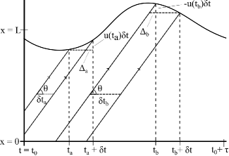
Figure 1: Spacetime diagram over one period of a moving wall’s motion. The smooth curve represents the wall’s position, and particles approach the wall along the diagonal arrows to collide at times $t_{a},t_{a}+\delta t,t_{b}$ and $t_{b}+\delta t$

The particle bouncing between the walls effectively measures the wall’s velocity during collisions, but the particle is not a stationary observer. Collisions with large relative speeds of approach occur more frequently than collisions with small relative speeds of approach, so there exists a statistical bias that favors collisions for which the wall moves towards the particle. If the quivering dynamics are to be physically consistent with the Fermi-Ulam dynamics, this statistical bias must be incorporated into the probability distribution used to determine the wall’s velocity during collisions. The mathematical realization of the statistical bias can be found with the aid of Fig. 1, a construction first employed by Hammersley Hammersley (1961) and Brahic Brahic (1970).
In Fig. 1, the position of the moving wall in the Fermi-Ulam model is plotted over one period of motion in the interval $(t_{0},t_{0}+\tau)$. Consider an ensemble of particles approaching the moving wall with speed $v$. For the moment, we assume that $v$ is larger than the maximum wall velocity $u_{max}$. The particles are launched from $x=0$ at a uniform rate over a period of duration $\tau$ such that they all collide with the wall during the interval $(t_{0},t_{0}+\tau)$. We concern ourselves only with the first collision each particle makes with the moving wall. Four trajectories from the ensemble are shown in Fig. 1, representing collisions with the wall at times $t_{a},\,t_{a}+\delta t,\,t_{b},$ and $t_{b}+\delta t$. Because the launch times are uniformly distributed, the fraction of particles that collide with the wall between $t_{a}$ and $t_{a}+\delta t$ will be proportional to the interval $\delta t_{a}=\delta t-\Delta_{a}$. Likewise, the fraction that collide between $t_{b}$ and $t_{b}+\delta t$ will be proportional to $\delta t_{b}=\delta t+\Delta_{b}$. Using the geometry of Fig. 1 and the fact that $\tan(\theta)=v$, we find the probability density for randomly selected ensemble member collide with the moving wall at a time $t$ within the interval $(t_{0},t_{0}+\tau)$ to be

$$P\boldsymbol{(}u(t)|v\boldsymbol{)}=\frac{1}{\tau}\left(1-\frac{u(t)}{v}\right).$$ (5)

Multiplying by a delta function and integrating Eq. (5) over a period of the wall’s motion gives $P(u|v)$, the probability density for a randomly selected ensemble member’s collision to occur when the wall moves with velocity $u$:

$$P(u|v) = \frac{1}{\tau}\int\limits_{0}^{\tau}\mathrm{d}t\,\delta\boldsymbol{(}u-u(t)\boldsymbol{)}\left(1-\frac{u(t)}{v}\right)$$

$$= \int\limits_{0}^{1}\mathrm{d}\Psi\,\delta\boldsymbol{(}u-u_{c}\,h^{\prime}(\Psi)\boldsymbol{)}\left(1-\frac{u_{c}\,h^{\prime}(\Psi)}{v}\right)$$

$$= P(u|0)\left(1-\frac{u}{v}\right).$$

Because the wall’s average displacement over one period of motion is zero, the product $uP(u|0)$ integrated over all wall velocities must also give zero, and $P(u|v)$ is therefore normalized and a well-defined probability density. The distribution $P(u|v)$ has a statistical bias towards larger negative $u$ due to the flux factor $1-u/v$. We will henceforth refer to $P(u|0)$ as the unbiased distribution and $P(u|v)$ as the biased distribution. In the quivering limit, $P(u|v)$ remains well-defined and unchanged. As $\tau\rightarrow 0$, an ensemble of particles launched over a period of wall motion from a fixed $x$ is essentially equivalent to an ensemble of infinitesimally displaced initial conditions. We therefore take $P(u|v)$ to be the conditional probability density to observe a quivering wall with velocity $u$ during a collision, given that the particle approaches the wall with speed $v>u_{max}$.
If a particle approaches the moving wall with speed $v<u_{max}$, then $P(u|v)$ will become negative for some values of $u$, and Eq. (II.1) will make no sense as a probability density. These $u$ values correspond to impossible collisions for which the wall moves with positive velocity away from the particle faster than the particle moves toward the wall. Such collisions occur with probability zero, and we can account for this by simply attaching a step-function to the biased distribution, yielding

$$P(u|v)=\begin{cases}P(u|0)\left(1-\frac{u}{v}\right),&v\geq u_{max}\\ N(v)P(u|0)\left(1-\frac{u}{v}\right)\Theta(v-u),&v<u_{max},\end{cases}$$ (7)

where $\Theta(x)$ is the unit step function (equal to $0$ for $x<0$ and $1$ for $x\geq 0$) and $N(v)$ is a $v$ dependent normalization.
Equation (7) determines the statistics of a particle’s energy evolution in a quivering Fermi-Ulam system. As with any billiard system, the particle’s energy is simply the kinetic energy $\frac{1}{2}mv^{2}$, where $m$ is the particle’s mass and $v$ is its speed. The particle bounces between the two walls as if the system were time-independent, but when colliding with the quivering wall at an incoming speed $v_{i}$ (the particle moves in the positive $x$ direction to collide with the moving wall, so $v_{i}$ is also the incoming velocity), a value for the wall velocity $u$ is selected using the biased distribution $P(u|v_{i})$. The particle’s velocity just after the collision, $v_{f}$, is given by

$$v_{f}=2u-v_{i},$$ (8)

and the corresponding energy change, $\Delta E$, is given by

$$\Delta E=2mu^{2}-2mu\,v_{i}.$$ (9)

Equations (8) and (9) are determined using the standard collision kinematics for a particle in one-dimension colliding elastically with an infinitely massive moving object.
Before moving on to higher dimensions, we must address the possibility of particles escaping the billiard interior. This issue will plague any fixed wall simplification of time-dependent billiards, and is discussed in detail in Ref. Karlis et al. (2008). From Eq. (8), we see that if $0<u<v_{i}\leq 2u$, the particle does not turn around after a collision with the moving wall, but instead slows down and continues forward. We refer to these types of collisions as glancing collisions. For non-zero $a$ and $\tau$, just after a glancing collision, the particle continues forward slower than the wall moves outward, so the particle will remain within the billiard interior. With a fixed wall simplification, however, the wall does not actually move outward after a glancing collision, so the particle will continue forward and escape the billiard interior. A particle escaping through a hard wall is a non-physical by-product of setting $a=0$, so in order to make a physically reasonable fixed wall simplification, one must always devise a method to handle glancing collisions. Our method for a quivering Fermi-Ulam system is devised as follows.
For non-zero $a$ and $\tau$, after a glancing collision occurs, the wall continues to evolve through its period, and one of two possibilities will occur. The wall may slow down sometime after the glancing collision and allow the particle to catch up and collide again, or the wall may reverse its direction and move inward sometime after the glancing collision, also allowing the particle to collide again. In either case, a second collision occurs after the first collision, and as $a$ and $\tau$ approach zero, the second occurs essentially instantaneously after the first. Therefore, we treat a glancing collision in a quivering Fermi-Ulam billiard as a double collision. When a particle with speed $v_{i}$ (also the particle’s velocity) collides with the quivering wall, we draw a $u$ value from the distribution $P(u|v_{i})$. If the selected value of $u$ is such that $0<u<v_{i}\leq 2u$, the particle’s new speed $v_{f}$ (also velocity) is given by $v_{f}=2u-v_{i}$, and we draw a new $u$ value from the distribution $P(u|v_{f})$. If the second $u$ value gives another glancing collision, we again update the particle’s speed and then draw a third $u$ value. The process is repeated until a non-glancing collision occurs, and the whole event (which occurs instantaneously) is treated as a single collision.

II.2 Arbitrary Time-Dependent Billiards

We now generalize to arbitrary billiards in arbitrary dimensions. Consider a time-dependent billiard in $d$ dimensions moving periodically through some continuous sequence of shapes with period $\tau$, characteristic oscillation amplitude $a$, and characteristic speed $u_{c}=a/\tau$. The evolution of any one point on the boundary will be denoted by the path $\mathbf{q}(t)$, where $\mathbf{q}(t+\tau)=\mathbf{q}(t)$. For every $t$, the set of all boundary points $\{\mathbf{q}(t)\}$ is assumed to define a collection of unbroken $d-1$ dimensional surfaces, which we refer to as the boundary components, enclosing some $d$ dimensional bounded connected volume. The outward unit normal to the billiard boundary at the point $\mathbf{q}(t)$ is denoted by $\mathbf{\hat{n}}\boldsymbol{(}\mathbf{q}(t)\boldsymbol{)}$, and the velocity of the boundary point $\mathbf{q}(t)$ is denoted by $\mathbf{u}\boldsymbol{(}\mathbf{q}(t)\boldsymbol{)}=\mathrm{d}\mathbf{q}(t)/\mathrm{d}t$. The billiard shape evolves continuously in time, and we assume that the boundary components remain unbroken throughout their evolution, so $\mathbf{u}\boldsymbol{(}\mathbf{q}(t)\boldsymbol{)}$ forms a smooth vector field with domain on the boundary $\{\mathbf{q}(t)\}$ for any fixed $t$. Likewise, $\mathbf{\hat{n}}\boldsymbol{(}\mathbf{q}(t)\boldsymbol{)}$ forms a smooth field on $\{\mathbf{q}(t)\}$ for any fixed $t$, except possibly at corners, where $\mathbf{\hat{n}}\boldsymbol{(}\mathbf{q}(t)\boldsymbol{)}$ is ill-defined and discontinuous. We denote the outward normal velocity of the point $\mathbf{q}(t)$ by $u\boldsymbol{(}\mathbf{q}(t)\boldsymbol{)}=\mathbf{u}\boldsymbol{(}\mathbf{q}(t)\boldsymbol{)}\cdot\mathbf{\hat{n}}\boldsymbol{(}\mathbf{q}(t)\boldsymbol{)}$.
Denote by $\mathbf{q}$ the average of $\mathbf{q}(t)$ over one period:

$$\mathbf{q}=\frac{1}{\tau}\int_{0}^{\tau}\mathrm{d}{t}\,\mathbf{q}(t).$$ (10)

Noting that the boundary components remain unbroken throughout the period of motion, it is straightforward to show that set of average boundary points $\{\mathbf{q}\}$ forms a collection of unbroken $d-1$ dimensional surfaces. The trajectory $\mathbf{q}(t)$ and normal velocity $u\boldsymbol{(}\mathbf{q}(t)\boldsymbol{)}$ of any given boundary point can be written as functions of the corresponding average location $\mathbf{q}$ and the time $t$:

$$\mathbf{q}(t) = \mathbf{q}+\mathbf{g}(\mathbf{q},t)$$ (11)

$$u(\mathbf{q},t) = \partial_{t}\mathbf{g}(\mathbf{q},t)\cdot\mathbf{\hat{n}}\boldsymbol{(}\mathbf{q}(t)\boldsymbol{)},$$

where $\mathbf{g}(\mathbf{q},t)$ is a piecewise smooth in time $\tau$ periodic function with a time average of zero. $\mathbf{g}(\mathbf{q},t)$ scales like $a$ and $u\boldsymbol{(}\mathbf{q}(t)\boldsymbol{)}$ scales like $u_{c}$. Equation (11) depends on $t$ only through the value of $\Psi(t)=t/\tau~{}\mathrm{mod}~{}1$, so we write

$$\mathbf{q}(t) = \mathbf{q}+a\,\mathbf{h}\boldsymbol{(}\mathbf{q},\Psi(t)\boldsymbol{)}$$ (12)

$$u(\mathbf{q},t) = u_{c}\,\partial_{\Psi}\mathbf{h}\boldsymbol{(}\mathbf{q},\Psi(t)\boldsymbol{)}\cdot\mathbf{\hat{n}}\boldsymbol{(}\mathbf{q}(t)\boldsymbol{)}.$$

where $a\,\mathbf{h}\boldsymbol{(}\mathbf{q},\Psi(t)\boldsymbol{)}=\mathbf{g}(\mathbf{q},t)$. Analogously to the one dimensional case, $\mathbf{h}$ is regarded as a function of $\mathbf{q}$ and $\Psi$, and $\mathbf{h}\boldsymbol{(}\mathbf{q},\Psi(t)\boldsymbol{)}$ means $\mathbf{h}(\mathbf{q},\Psi)$ evaluated for $\Psi=\Psi(t)$. The quivering limit of an arbitrary dimensional billiard is defined by taking $a,\tau\rightarrow 0$ while holding $u_{c}$ and the dependence of $\mathbf{h}$ on $\Psi$ and $\mathbf{q}$ constant. In this limit, the billiard’s boundary points become fixed in time at the average locations $\{\mathbf{q}\}$, so the outward normal vectors become fixed in time as well. Thus, in the quivering limit, we have

$$\mathbf{q}(t) = \mathbf{q}$$ (13)

$$u(\mathbf{q},t) = u_{c}\,\partial_{\Psi}\mathbf{h}\boldsymbol{(}\mathbf{q},\Psi(t)\boldsymbol{)}\cdot\mathbf{\hat{n}}(\mathbf{q})$$

$$= u_{c}\,h^{\prime}\boldsymbol{(}\mathbf{q},\Psi(t)\boldsymbol{)},$$

where we write $h^{\prime}\boldsymbol{(}\mathbf{q},\Psi(t)\boldsymbol{)}=\partial_{\Psi}\mathbf{h}\boldsymbol{(}\mathbf{q},\Psi(t)\boldsymbol{)}\cdot\mathbf{\hat{n}}(\mathbf{q})$ for brevity. Any time-dependent billiard taken to the quivering limit will be called a quivering billiard.
Analogously to the one dimensional case, we define the unbiased distribution for each $\mathbf{q}$:

$$P(u|0,\mathbf{q})=\int_{0}^{1}\mathrm{d}\Psi\delta\boldsymbol{(}u-u_{c}\,h^{\prime}(\mathbf{q},\Psi)\boldsymbol{)}.$$ (14)

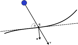
Figure 2: Collision geometry in a two-dimensional billiard. A particle with velocity $\mathbf{v}$ approaches the point $\mathbf{q}$ on the billiard boundary, where the outward unit normal vector is $\mathbf{n}$. The dotted line represents the tangent line to the boundary at $\mathbf{q}$

The biased distribution for each $\mathbf{q}$ can also be defined analogously to the one dimensional case, but we must also consider the collision angle $\theta$, depicted for two-dimensional billiard in Fig. 2. For a particle approaching the boundary point $\mathbf{q}$ with speed $v$, $\theta$ is the angle between the particle’s velocity vector and the $d-1$ dimensional tangent surface to the wall at $\mathbf{q}$, and $v\sin(\theta)$ thus gives the component of the particle’s velocity in the $\mathbf{\hat{n}}(\mathbf{q})$ direction. If the particle collides when the wall has normal velocity $u$, then the relative speed of approach just before the collision is determined by $v\sin(\theta)$ and $u$, so $v\sin(\theta)$ determines the statistical bias towards collisions with large negative $u$. We account for this by simply replacing $v$ with $v\sin(\theta)$ in Eq. (7), yielding

$$P(u|v,\mathbf{q},\theta)=\begin{cases}P(u|0,\mathbf{q})\left(1-\frac{u}{v\sin(\theta)}\right),&v\sin(\theta)\geq u_{max}(\mathbf{q})\\ N(v,\theta)P(u|0,\mathbf{q})\left(1-\frac{u}{v\sin(\theta)}\right)\Theta\boldsymbol{(}v\sin(\theta)-u\boldsymbol{)},&v\sin(\theta)<u_{max}(\mathbf{q}),\end{cases}$$ (15)

Equation (15) determines the statistics of a particle’s energy evolution in a quivering billiard.
To summarize, we describe how one may construct a quivering billiard and determine a particle’s trajectory, without the need to define a real, fully time-dependent billiard and take the quivering limit. First, one must select a billiard shape by defining a surface $\{\mathbf{q}\}$, then set boundary quivering by giving a value to $u_{c}$ and defining a scalar field $h^{\prime}(\mathbf{q},\Psi)$ on $\{\mathbf{q}\}$. If the constructed quivering billiard is to honestly represent some deterministic billiard’s motion in the quivering limit, then $h^{\prime}(\mathbf{q},\Psi)$ should be chosen to be a smooth function of $\mathbf{q}$ for any $\Psi$ wherever $\mathbf{\hat{n}}(\mathbf{q})$ in continuous. Using the field $h^{\prime}$ and the value of $u_{c}$, one may then calculate the unbiased distribution $P(u|0,\mathbf{q})$ from Eq. (14) for any $\mathbf{q}$ on the billiard boundary. For a particle in free flight inside the quivering billiard, the next collision location is found deterministically using the geometry of the billiard boundary, just as with a time-independent billiard. When a particle with velocity $\mathbf{v}_{i}$ and speed $v_{i}$ collides with the boundary at $\mathbf{q}$ with a collision angle $\theta_{i}$, we draw a value of $u$ from the distribution $P(u|v_{i},\mathbf{q},\theta_{i})$. The particle’s velocity component tangent to the boundary remains constant, and the component normal to the boundary just after the collision, $\mathbf{v}_{f}\cdot\hat{\mathbf{n}}(\mathbf{q})$, is given by

$$\mathbf{v}_{f}\cdot\hat{\mathbf{n}}(\mathbf{q}) = 2u-\mathbf{v}_{i}\cdot\hat{\mathbf{n}}(\mathbf{q})$$

$$= 2u-v_{i}\sin(\theta_{i}).$$

The corresponding change in energy, $\Delta E$, is given by

$$\Delta E=2mu^{2}-2mu\,v_{i}\sin\left(\theta_{i}\right).$$ (17)

Analogously to the one dimensional case, if the selected value of $u$ is such that $0<u<v_{i}\sin(\theta_{i})\leq 2u$, then a glancing collision occurs, and we draw a second value of $u$ using the same collision located and updated particle speed and collision angle, determined from Eqs. (II.2) and (17).

III Energy Statistics

In this section, we study in detail the statistical behavior of particles and ensembles in a $d$-dimensional quivering billiard, with the aim of describing energy evolution of a ensemble of initial conditions as a diffusion process. Our notation will be as follows: $\mathbf{q}_{b}$ is the location of a particle’s $b^{th}$ collision with the billiard boundary, $\theta_{b}$ is the $b^{th}$ collision angle, $u_{b}$ is the selected value of the wall velocity during the $b^{th}$ collision (sampled using Eq. (15)), $v_{b-1}$ is the particle’s speed just before the $b^{th}$ collision, and $\Delta E_{b}$ is the change in particle energy due to the $b^{th}$ collision, given by

$$\Delta E_{b}=2mu_{b}^{2}-2mu_{b}\,v_{b-1}\sin\left(\theta_{b}\right).$$ (18)

In order to derive analytic results, we will assume that the initial particle speeds $v_{0}$ are much larger than $u_{c}$, and we will solve to leading order in the small parameter $\varepsilon=u_{c}/v_{0}$. We regard $u_{c}$ as an $O(1)$ quantity, and $v_{0}$ as an $O(\varepsilon^{-1})$ quantity. This approximation allows us to ignore glancing collisions in our analysis, and also allows us ignore the possibility of $v_{b-1}\sin(\theta_{b})\leq u_{max}(\mathbf{q}_{b})$, so that the biased distributions at the time of collision always take the form $P(u_{b}|v_{b-1},\mathbf{q}_{b},\theta_{b})=P(u_{b}|0,\mathbf{q}_{b})\left(1-u_{b}/v_{b-1}\sin(\theta_{b})\right)$ (as opposed to the more complicated Eq. (15)). The assumption $\varepsilon\ll 1$ is not particularly restrictive; even if particles begin with an initial speed comparable to or less than $u_{c}$, energy gaining collisions are more likely than energy losing collisions due to the flux factor in the biased distribution, and a slow particle will gain roughly $mu_{c}^{2}$ of energy during a collision according to Eq. (18). Therefore, a slow particle will more than likely gain speed $u_{c}\sim O(1)$ during a single bounce, and after $1/\delta$ bounces, where $\delta\ll 1$ is some small number, the particle will more than likely have a speed $v$ such that $u_{c}/v\lesssim\delta\ll 1$. Thus, slow particles are very likely to eventually become fast particles, and the assumption $u_{c}/v\ll 1$ will give a better and better approximation over time.
In the analysis, it will prove useful to consider both the full dynamics and frozen dynamics, as is done in Refs. Jarzynski (1992, 1993). If the frozen dynamics are used at the $b^{th}$ collision, the energy change $\Delta E_{b}$ is calculated, but the particle’s energy remains constant, and the angle of reflection is equal to the collision angle $\theta_{b}$. In other words, the frozen dynamics are identical to those of a time-independent billiard, but we calculate and keep track of the $\Delta E_{b}$’s that would have occurred had the billiard walls been quivering. In the full dynamics, the particle’s energy is actually incremented by the calculated value of $\Delta E_{b}$, and the angle of reflection is consequently altered.

III.1 Expectations

Consider single a particle with energy $E_{0}$ released at time $t_{0}$ in a $d$-dimensional quivering billiard. The resulting particle trajectory generates a sequence of energy increments $\{\Delta E_{1},\Delta E_{2},...,\Delta E_{b-1},\Delta E_{b},\Delta E_{b+1},...\}$. Let the operator $\{...\}_{b}$ denote the conditional expectation value of the quantity $...$, given the outcomes of the previous $b-1$ bounces. The first $b-1$ bounces determine $v_{b-1}$, $\mathbf{q}_{b}$, and $\theta_{b}$, so the $b^{th}$ conditional expected energy change, $\mu_{b}\equiv\{\Delta E_{b}\}_{b}$, can be calculated using the biased distribution $P(u_{b}|v_{b-1},\mathbf{q}_{b},\theta_{b})$ and the expression for $\Delta E_{b}$ in Eq. (18):

$$\mu_{b} \equiv \{\Delta E_{b}\}_{b}$$

$$= \int\mathrm{d}u_{b}P(u_{b}|v_{b-1},\mathbf{q}_{b},\theta_{b})\Delta E_{b}$$

$$= \int\mathrm{d}u_{b}P(u_{b}|0,\mathbf{q}_{b})\left(4mu_{b}^{2}-\frac{2mu_{b}^{3}}{v_{b-1}\sin(\theta_{b})}-2mu_{b}\,v_{b-1}\sin(\theta_{b})\right).$$

The integral in Eq. (III.1) is taken over all possible values of $u_{b}$ at $\mathbf{q}_{b}$.
Let $M_{n}(\mathbf{q}_{b})$ denote the $n^{th}$ moment of the wall velocity at $\mathbf{q}_{b}$ as measured by a stationary observer:

$$M_{n}(\mathbf{q})=\int\mathrm{d}uP(u|0,\mathbf{q})u^{n}.$$ (20)

By construction, $M_{1}(\mathbf{q})=0$ for all $\mathbf{q}$. Otherwise, $M_{n}(\mathbf{q}_{b})$ generally scales like $u_{c}^{n}$. The conditional mean thus simplifies to

$$\mu_{b} = \int\mathrm{d}u_{b}P(u_{b}|0,\mathbf{q}_{b})4mu_{b}^{2}\left(1-\frac{u_{b}}{2v_{b-1}\sin(\theta_{b})}\right)$$

$$= 4mM_{2}(\mathbf{q}_{b})\left(1-\frac{M_{3}(\mathbf{q}_{b})/M_{2}(\mathbf{q}_{b})}{2v_{b-1}\sin(\theta_{b})}\right).$$

Similarly, the conditional variance $\sigma_{b}^{2}$ is given by

$$\sigma_{b}^{2} \equiv \{(\Delta E_{b})^{2}\}_{b}-\{\Delta E_{b}\}^{2}_{b}$$

$$= \int\mathrm{d}u_{b}P(u_{b}|v_{b-1},\mathbf{q}_{b},\theta_{b})\left((\Delta E_{b})^{2}-\{\Delta E_{b}\}^{2}_{b}\right)$$

$$= 4m^{2}[M_{2}(\mathbf{q}_{b})]^{2}\left(\frac{v_{b-1}^{2}\sin^{2}(\theta_{b})}{M_{2}(\mathbf{q}_{b})}-3\frac{v_{b-1}\sin(\theta_{b})}{[M_{2}(\mathbf{q}_{b})]^{2}/M_{3}(\mathbf{q}_{b})}+~{}3\frac{M_{4}(\mathbf{q}_{b})}{[M_{2}(\mathbf{q}_{b})]^{2}}\right.$$

$$~{}\left.-4+\frac{4M_{3}(\mathbf{q}_{b})/M_{2}(\mathbf{q}_{b})-M_{5}(\mathbf{q}_{b})/[M_{2}(\mathbf{q}_{b})]^{2}}{v_{b-1}\sin(\theta_{b})}-\frac{[M_{3}(\mathbf{q}_{b})]^{2}/[M_{2}(\mathbf{q}_{b})]^{2}}{v_{b-1}^{2}\sin^{2}(\theta_{b})}\right).$$

The terms enclosed in the parentheses of Eqs. (III.1) and (III.1) are ordered in increasing powers of $\varepsilon$. To leading order, we have

$$\mu_{b}=4mM_{2}(\mathbf{q}_{b})$$ (23)

$$\sigma_{b}^{2}=4m^{2}M_{2}(\mathbf{q}_{b})v_{b-1}^{2}\sin^{2}(\theta_{b})$$

The quantities $\mu_{b}$ and $\sigma^{2}_{b}$ are $O(1)$ and $O\left(\varepsilon^{-2}\right)$, respectively; average energy gain is moderate, and fluctuations are huge.

III.2 Correlations

The conditional covariance between adjacent bounces, $\mathrm{Cov}_{b,b+1}$, is defined by

$$\mathrm{Cov}_{b,b+1} \equiv \left\{\left(\Delta E_{b}-\{\Delta E_{b}\}_{b}\right)\left(\Delta E_{b+1}-\{\Delta E_{b+1}\}_{b}\right)\right\}_{b}$$

$$= \{\Delta E_{b}\Delta E_{b+1}\}_{b}-\{\Delta E_{b}\}_{b}\{\Delta E_{b+1}\}_{b}.$$

The conditional expectations in Eq. (III.2) are taken given the outcomes of the previous $b-1$ collisions, with the outcome of the $b^{th}$ collision yet to be determined. That is, we must average over all possible realizations of the stochastic process $E_{b-1}\rightarrow E_{b-1}+\Delta E_{b}\rightarrow E_{b-1}+\Delta E_{b}+\Delta E_{b+1}$, given the first $b-1$ collisions. Denote $\{\Delta E_{b+1}|u_{b}\}_{b+1}$ as the conditional expectation of $E_{b+1}$, given the first $b-1$ collision outcomes and supposing that $u_{b}$ is the wall velocity during the $b^{th}$ collision. The expression for $\{\Delta E_{b+1}\}_{b}$ is then

$$\{\Delta E_{b+1}\}_{b}=\int\mathrm{d}u_{b}P(u_{b}|v_{b-1},\mathbf{q}_{b},\theta_{b})\{\Delta E_{b+1}|u_{b}\}_{b+1}.$$ (25)

The expression for $\{\Delta E_{b}\Delta E_{b+1}\}_{b}$ can be written similarly:

$$\{\Delta E_{b}\Delta E_{b+1}\}_{b} = \int\mathrm{d}u_{b}\mathrm{d}u_{b+1}P(u_{b}|v_{b-1},\mathbf{q}_{b},\theta_{b})P(u_{b+1}|v_{b},\mathbf{q}_{b+1},\theta_{b+1}|u_{b})\Delta E_{b}\Delta E_{b+1}$$

$$= \int\mathrm{d}u_{b}P(u_{b}|v_{b-1},\mathbf{q}_{b},\theta_{b})\Delta E_{b}\{\Delta E_{b+1}|u_{b}\}_{b+1}.$$

The term $P(u_{b+1}|v_{b},\mathbf{q}_{b+1},\theta_{b+1}|u_{b})$ denotes the value of $P(u_{b+1}|v_{b},\mathbf{q}_{b+1},\theta_{b+1})$ when $v_{b},\theta_{b+1}$, and $\mathbf{q}_{b+1}$ are determined given the first $b-1$ collision outcomes while supposing that $u_{b}$ is the wall velocity upon the $b^{th}$ collision. Equation (III.2) can thus be expressed as

$$\mathrm{Cov}_{b,b+1}=\int\mathrm{d}u_{b}P(u_{b}|v_{b-1},\mathbf{q}_{b},\theta_{b})\{\Delta E_{b+1}|u_{b}\}_{b+1}\left(\Delta E_{b}-\{\Delta E_{b}\}_{b}\right).$$ (27)

If the frozen dynamics are used at the $b^{th}$ collision, then $v_{b}$, $\theta_{b+1}$, and $\mathbf{q}_{b+1}$ are independent of $u_{b}$, so we have

$$\{\Delta E_{b+1}|u_{b}\}_{b+1}|_{F}=\{\Delta E_{b+1}\}_{b+1}|_{F}=\mu_{b+1}|_{F},$$ (28)

where $...|_{F}$ denotes the quantity $...$ evaluated using the frozen dynamics. $\mu_{b+1}|_{F}$ carries no $u_{b}$ dependence, so it can be brought outside of the integral in Eq. (27), giving

$$\mathrm{Cov}_{b,b+1}|_{F}=0.$$ (29)

Adjacent energy increments are thus statistically uncorrelated in the frozen dynamics.
Under the assumption $\varepsilon\ll 1$, the frozen dynamics closely resemble the full dynamics over the time scale of a few bounces Jarzynski (1993). Over such a time scale, we can regard the full dynamics trajectory as a stochastic perturbation of the deterministic frozen dynamics trajectory. Let $\mathbf{q}_{b+1}|u_{b}=\mathbf{q}_{b+1}|_{F}+\delta\mathbf{q}_{b+1}|u_{b}$ be the $(b+1)^{th}$ collision location when the full dynamics are used at the $b^{th}$ bounce, given the first $b-1$ collisions and supposing that $u_{b}$ is the observed wall velocity upon the $b^{th}$ collision. Equation (23) then gives, to leading order in $\varepsilon$

$$\{\Delta E_{b+1}|u_{b}\}_{b+1} = 4mM_{2}(\mathbf{q}_{b+1}|u_{b})$$

$$= 4mM_{2}(\mathbf{q}_{b+1}|_{F})+4m\,\nabla M_{2}(\mathbf{q}_{b+1}|_{F})\cdot\delta\mathbf{q}_{b+1}|u_{b}.$$

where the gradient $\nabla M_{2}$ is constrained to act along directions tangent to the billiard boundary at $\mathbf{q}_{b+1}|_{F}$. In the appendix, we solve for $\|\delta\mathbf{q}_{b+1}|u_{b}\|$ to leading order in $\varepsilon$ and find

$$\|\delta\mathbf{q}_{b+1}|u_{b}\|=2L_{b}|_{F}\frac{\cos(\theta_{b})}{\sin(\theta_{b+1}|_{F})}\frac{|u_{b}|}{v_{b-1}},$$ (31)

where $L_{b}|_{F}$ is the distance between the $b^{th}$ and $b+1^{th}$ collision locations in the frozen dynamics. Combining Eqs. (27), (III.2), and (31), gives to leading order in $\varepsilon$

$$\mathrm{Cov}_{b,b+1} = \int\mathrm{d}u_{b}P(u_{b}|v_{b-1},\mathbf{q}_{b},\theta_{b})\left(4m\,\nabla M_{2}(\mathbf{q}_{b+1}|_{F})\cdot\delta\mathbf{q}_{b+1}|u_{b}\right)\left(\Delta E_{b}-\{\Delta E_{b}\}_{b}\right)$$

$$= \int\mathrm{d}u_{b}P(u_{b}|0,\mathbf{q}_{b})\left(4m\nabla M_{2}(\mathbf{q}_{b+1}|_{F})\cdot\frac{\delta\mathbf{q}_{b+1}|u_{b}}{\|\delta\mathbf{q}_{b+1}|u_{b}\|}\right.$$

$$\times~{}\left.2L_{b}|_{F}\frac{\cos(\theta_{b})}{\sin(\theta_{b+1}|_{F})}\frac{|u_{b}|}{v_{b-1}}\right)\left(4mu_{b}^{2}-2m\frac{u_{b}^{3}}{v_{b-1}\sin(\theta_{b})}-2mu_{b}v_{b-1}\sin(\theta_{b})\right.$$

$$\left.-4mM_{2}(\mathbf{q}_{b})+4mM_{2}(\mathbf{q}_{b})\frac{u_{b}}{v_{b-1}\sin(\theta_{b})}\right)$$

$$= -16m^{2}L_{b}|_{F}\frac{\cos(\theta_{b})\sin(\theta_{b})}{\sin(\theta_{b+1}|_{F})}\nabla M_{2}(\mathbf{q}_{b+1}|_{F})\cdot\int\mathrm{d}u_{b}P(u_{b}|0,\mathbf{q}_{b})\frac{\delta\mathbf{q}_{b+1}|u_{b}}{\|\delta\mathbf{q}_{b+1}|u_{b}\|}u_{b}|u_{b}|.$$

All but the leading order terms are dropped in the last line of Eq. (III.2). With exception to the one-dimensional case, $\mathrm{Cov}_{b,b+1}$ is thus an $O(1)$ quantity. In a one-dimensional billiard, the frozen and full dynamics always give the same collision location, so $\{\Delta E_{b+1}|u_{b}\}_{b+1}=\{\Delta E_{b+1}\}_{b+1}|_{F}$, and consequently, $\mathrm{Cov}_{b,b+1}$ is identically zero.
The conditional correlation $\rho_{b,b+1}$ is defined as the normalized conditional covariance, and is given by

$$\rho_{b,b+1}=\frac{\mathrm{Cov}_{b,b+1}}{\sigma_{b}\{\sigma_{b+1}\}_{b}}.$$ (33)

To leading order in $\varepsilon$, the conditional expectation $\{\sigma_{b+1}\}_{b}$ can be taken as the frozen dynamics value in Eq. (33). Therefore, the conditional correlation $\rho_{b,b+1}$ is $O(\varepsilon^{2})$ (with exception to the one-dimensional case, where $\rho_{b,b+1}=0$). This quantity is very small, and correlations between more distant collisions will further diminish due to the mixing of particle trajectories induced by the stochastic wall motion. We thus conclude that, in any dimension, correlations between energy increments effectively decay over the time scale of a single collision.

III.3 Ensemble averages

Consider now a microcanonical ensemble of independent particles with energy $E_{0}$ released at time $t_{0}$. The resulting trajectories will generate an ensemble of statistically independent energy increment sequences, and we denote $\Delta E_{i,b}$ as the $b^{th}$ recorded energy increment of the $i^{th}$ particle. Define the ensemble averaged $b^{th}$ energy increment $\left<\Delta E_{b}\right>$ as

$$\left<\Delta E_{b}\right>\underset{N\rightarrow\infty}{=}\sum\limits_{i=1}^{N}\frac{\Delta E_{i,b}}{N},$$ (34)

and the ensemble averaged $b^{th}$ conditional mean $\left<\mu_{b}\right>$ as

$$\left<\mu_{b}\right>\underset{N\rightarrow\infty}{=}\sum\limits_{i=1}^{N}\frac{\mu_{i,b}}{N},$$ (35)

where $\mu_{i,b}=\{\Delta E_{i,b}\}_{b}$. Equation (III.1) shows that the $b^{th}$ conditional variances $\sigma_{i,b}^{2}\equiv\{\left(\Delta E_{i,b}\right)^{2}\}_{b}-\{\Delta E_{i,b}\}^{2}$ are finite and bounded from above. Noting this, and the fact that the series $\sum\limits_{k=1}^{\infty}k^{-2}$ converges, we deduce

$$\lim\limits_{N\rightarrow\infty}\sum\limits_{k=1}^{N}\frac{\sigma_{k,b}^{2}}{k^{2}}<\infty.$$ (36)

By Kolmogorov’s strong law of large numbers Revesz (1968), Eq. (36) assures that, with probability unity,

$$\left<\Delta E_{b}\right>=\left<\mu_{b}\right>.$$ (37)

Combining Eqs. (37),(35), and (23) gives, to leading order in $\varepsilon$,

$$\left<\Delta E_{b}\right> \underset{N\rightarrow\infty}{=} \sum\limits_{i=1}^{N}\frac{4mM_{2}(\mathbf{q}_{i,b})}{N}$$

$$= 4m\left<M_{2}(\mathbf{q}_{b})\right>,$$

where $\mathbf{q}_{i,b}$ denotes the $b^{th}$ collision location of the $i^{th}$ particle. By similar law of large number arguments, we also have, to leading order in $\varepsilon$,

$$\left<u_{b}^{2}\right>=\left<M_{2}(\mathbf{q}_{b})\right>,$$ (39)

where

$$\left<u_{b}^{2}\right>\underset{N\rightarrow\infty}{=}\sum\limits_{i=1}^{N}\frac{u_{i,b}^{2}}{N},$$ (40)

and $u_{i,b}$ is the wall velocity during the $b^{th}$ collision of the $i^{th}$ particle. To leading order, we thus have

$$\left<\Delta E_{b}\right>=4m\left<u_{b}^{2}\right>.$$ (41)

III.4 Energy diffusion

We now consider the normalized energy distribution of an ensemble of independent particles, denoted by $\eta(E,t)$. We have thus far shown that energy of any one ensemble member evolves stochastically, in small increments, with correlations in energy changes effectively decaying over a characteristic time scale given by time between collisions. A particle’s energy evolution is therefore effectively a Markov process describing a random walk along an energy axis, so following Refs. Wilkinson (1990); Jarzynski (1993), we assert that $\eta(E,t)$ evolves like a diffusion process and obeys a Fokker-Planck equation:

$$\partial_{t}\eta(E,t)=-\partial_{E}\left[g_{1}(E,t)\eta(E,t)\right]+\frac{1}{2}\partial^{2}_{E}\left[g_{2}(E,t)\eta(E,t)\right].$$ (42)

The functions $g_{1}(E,t)$ and $g_{2}(E,t)$, the drift and diffusion terms, respectively, are to be determined in this section. The energy of any one particle in a quivering billiard evolves discretely in time, so the continuous time evolution implied by Eq. (42) will be an accurate description of the ensemble only down to a coarse-grained time scale. The time scale must be large enough to ensure that most particles in the ensemble experience at least a few bounces off the billiard wall, but small enough to ensure the energy change experienced by most particles is small compared to their total energy. Generally speaking, a diffusive description of a stochastic process is only accurate over time scales larger than the process’s typical correlation time Jarzynski (1992, 1993). We have established that energy correlations for any one particle effectively decay over the time scale of a single collision, thus, the diffusion approach to energy evolution in a quivering billiard is justified on any time scale over which $\eta(E,t)$ can be described by a continuous evolution.
The drift term $g_{1}(E^{\prime},t^{\prime})$ is defined as the rate of ensemble averaged energy change for an ensemble of particles all with energy $E^{\prime}$ at time $t^{\prime}$. Specifically,

$$g_{1}(E^{\prime},t^{\prime})\underset{\Delta t\rightarrow 0}{=}\frac{\left<E(t^{\prime}+\Delta t)-E(t^{\prime})\right>}{\Delta t},$$ (43)

where $E(t^{\prime})=E^{\prime}$ for all particles in the ensemble, and $\left<E(t^{\prime}+\Delta t)\right>$ is the ensemble averaged particle energy at time $t^{\prime}+\Delta t$. We can not actually take the limit $\Delta t\rightarrow 0$ because $g_{1}$ has no meaning over time scales for which the evolution of $\eta$ appears discontinuous. Instead, we will let $\Delta t$ be the average time for which the ensemble members make $B$ bounces after time $t^{\prime}$, and we will find corresponding ensemble averaged change in energy. We assume that $B$ is small enough so that the particle energies change very little relative to $E^{\prime}$ over the time $\Delta t$, so that $\Delta t$ is the smallest coarse-grained time scale for which Eq. (42) is valid for an ensemble with common energy $E^{\prime}$. We let $E_{B}$ be a particle’s energy $B$ bounces after $t^{\prime}$, and find from Eq. (37)

$$\left<E_{B}-E^{\prime}\right> = \left<\sum\limits^{B}\Delta E_{b}\right>$$

$$= \sum\limits^{B}4m\left<u_{b}^{2}\right>.$$

We denote the coarse grained squared wall speed by $\overline{u^{2}}(t^{\prime};B)$, defined as the time average of $\left<u^{2}_{b}\right>$ over the first $B$ bounces after $t^{\prime}$:

$$\overline{u^{2}}(t^{\prime};B)=\sum\limits^{B}\frac{\left<u^{2}_{b}\right>}{B}.$$ (45)

We thus have

$$\left<E_{B}-E^{\prime}\right>=4m~{}\overline{u^{2}}(t^{\prime};B)B$$ (46)

The time scale $\Delta t$ corresponding to the $B$ bounces after $t^{\prime}$ is the ensemble averaged total free flight time over which the $B$ bounces occur. If we denote by $\Delta t_{b}$ a particle’s $b^{th}$ free flight time after $t^{\prime}$, we have

$$\Delta t=\sum\limits^{B}\left<\Delta t_{b}\right>.$$ (47)

We are assuming small wall velocities, so the particles’ speeds change very little relative to their initial speed $\sqrt{2E^{\prime}/m}$ over the $B$ bounces. Therefore, to leading order in $\varepsilon$, we have

$$\Delta t_{b}=\sqrt{\frac{m}{2E^{\prime}}}l_{b},$$ (48)

where $l_{b}$ denotes a particles $b^{th}$ free flight distance after $t^{\prime}$. We now define the coarse grained free flight distance, $\overline{l}(t^{\prime},B)$ by time averaging the ensemble average of $l_{b}$ over the first $B$ bounces after $t^{\prime}$:

$$\overline{l}(t^{\prime};B)=\sum\limits^{B}\frac{\left<l_{b}\right>}{B}$$ (49)

Substituting Eqs. (49) and (48) into Eq. (47) gives

$$\Delta t=B~{}\overline{l}(t^{\prime};B)\sqrt{\frac{m}{2E^{\prime}}},$$ (50)

and substituting for $B$ in Eq. (46) gives

$$\left<E_{B}-E^{\prime}\right>=\Delta t~{}\frac{4\sqrt{2m}~{}\overline{u^{2}}(t^{\prime};B)}{\overline{l}(t^{\prime};B)}E^{\prime\frac{1}{2}}.$$ (51)

Equation (51) gives the ensemble averaged change in energy over the time $\Delta t$ after $t^{\prime}$ for an ensemble of particles with energy $E^{\prime}$. Comparing to Eq. (43), we see that dividing both sides of Eq. (51) by $\Delta t$ gives us $g_{1}(E^{\prime},t^{\prime})$. We thus have,

$$g_{1}(E,t)=\frac{4\sqrt{2m}~{}\overline{u^{2}}(t)}{\overline{l}(t)}E^{\frac{1}{2}},$$ (52)

where we have switched from primed to unprimed variables, and the dependence on $B$ has been suppressed.
The diffusion term $g_{2}(E^{\prime},t^{\prime})$ is defined as

$$g_{2}(E^{\prime},t^{\prime})\underset{\Delta t\rightarrow 0}{=}\frac{\left<\left(E(t^{\prime}+\Delta t)-E(t^{\prime})\right)^{2}\right>}{\Delta t},$$ (53)

where $E(t^{\prime})=E^{\prime}$ for all particles in the ensemble, and $\left<E(t^{\prime}+\Delta t)\right>$ is the ensemble averaged particle energy at time $t^{\prime}+\Delta t$. An expression for the diffusion term can be found by employing similar methods used to find the drift term. Alternatively, $g_{2}(E,t)$ can be found by invoking Liouville’s theorem, as in Ref. Jarzynski (1992). Combing Liouville’s theorem and the Fokker-Planck equation allows one to deduce a fluctuation-dissipation relation:

$$g_{1}(E,t)=\frac{1}{2\Sigma(E)}\partial_{E}\left[\Sigma(E)g_{2}(E,t)\right],$$ (54)

where $\Sigma(E)$ is the microcanonical partition function of a single particle with energy $E$ in the corresponding frozen billiard. In a $d$ dimensional billiard, the microcanonical partition function is given by Jarzynski (1993)

$$\Sigma(E)=\frac{1}{2}V_{d}\,\Omega_{d}\left(2m\right)^{\frac{d}{2}}E^{\frac{d}{2}-1},$$ (55)

where $\Omega_{d}$ is the $d$-dimensional solid angle, and $V_{d}$ is the $d$-dimensional billiard’s volume. Combining Eqs. (52),(54), and (55), we find

$$g_{2}(E,t)=\frac{4}{d+1}\frac{4\sqrt{2m}~{}\overline{u^{2}}(t)}{\overline{l}(t)}E^{\frac{3}{2}}.$$ (56)

This method of determining $g_{2}$ allows for an additive constant, but this constant must be identically zero; when $E=0$, the particles are motionless and there can be no drift or diffusion of energies, so we must have $g_{1}(0,t)=g_{2}(0,t)=0$.
With our expressions for $g_{1}$ and $g_{2}$, we may rewrite the Fokker-Planck equation:

$$\partial_{t}\eta(E,t)=\frac{2\alpha(t)}{d+1}\partial_{E}\left[E^{\frac{1+d}{2}}\partial_{E}\left(E^{\frac{2-d}{2}}\eta(E,t)\right)\right]$$ (57)

where we define $\alpha(t)$ as

$$\alpha(t)\equiv\frac{4\sqrt{2m}~{}\overline{u^{2}}(t)}{\overline{l}(t)}.$$ (58)

Equation (57) can be simplified by defining a rescaled time $s$:

$$s=\int_{t_{0}}^{t}\mathrm{d}t^{\prime}\alpha(t^{\prime}),$$ (59)

which gives

$$\partial_{s}\eta(E,s)=\frac{2}{d+1}\partial_{E}\left[E^{\frac{1+d}{2}}\partial_{E}\left(E^{\frac{2-d}{2}}\eta(E,s)\right)\right]$$ (60)

Equation (60) can be solved by separation of variables. We assume a solution of the form $\phi(s)f(E)$, and upon making the substitutions $F(E)=E^{\frac{3-d}{4}}f(E)$ and $z=E^{\frac{1}{4}}$ one finds a first order homogeneous linear differential equation for $\phi(s)$ and a Bessel equation of order $d-1$ for $F(z)$. The details of the separation of variables, including existence, uniqueness, and boundary conditions, are given in Ref. Kargovsky et al. (2013) and will be omitted here. We also acknowledge a similar, much older, one-dimensional solution given in Ref. Zaslavskii and Chirikov (1965). The separation of variables solution is

$$\eta(E,s)=E^{\frac{d-3}{4}}\int_{0}^{\infty}\mathrm{d}k\,A(k)J_{d-1}(kE^{\frac{1}{4}})e^{-\frac{sk^{2}}{8(d+1)}},$$ (61)

where $J_{d-1}$ is an ordinary Bessel function of order $d-1$, and the amplitudes $A(k)$ are found by taking a Hankel transform of the initial ensemble $\eta(E,0)$. When the ensemble begins in the microcanonical distribution with energy $E_{0}$, we have $\eta(E,0)=\delta(E-E_{0})$, and a closed form expression for $A(k)$ results. The energy distribution $\eta(E,s)$, subject to $\eta(E,0)=\delta(E-E_{0})$, is then

$$\eta(E,s)=\frac{1}{4E_{0}^{\frac{1}{2}}}\left(\frac{E}{E_{0}}\right)^{\frac{d-3}{4}}\int_{0}^{\infty}\mathrm{d}k\,kJ_{d-1}(kE_{0}^{\frac{1}{4}})J_{d-1}(kE^{\frac{1}{4}})e^{-\frac{sk^{2}}{8(d+1)}}.$$ (62)

Making use of an identity of Bessel integrals utilized in Eq. (22) of Ref. Kargovsky et al. (2013), we can solve the integral in Eq. (62) and simplify the expression to

$$\eta(E,s)=\frac{d+1}{sE_{0}^{\frac{1}{2}}}\left(\frac{E}{E_{0}}\right)^{\frac{d-3}{4}}I_{d-1}\left[\frac{4(d+1)}{s}E_{0}^{\frac{1}{4}}E^{\frac{1}{4}}\right]e^{-\frac{2(d+1)}{s}\left(E_{0}^{\frac{1}{2}}+E^{\frac{1}{2}}\right)},$$ (63)

where $I_{d-1}$ is a modified Bessel function of order $d-1$. Using this energy distribution, we can find the ensemble averaged energy as a function of time:

$$\left<E(s)\right>=\frac{d}{d+1}\frac{s^{2}}{4}+\sqrt{E_{0}}~{}s+E_{0}.$$ (64)

Equation (63) is only valid under the assumption $\varepsilon\ll 1$. If we begin with an ensemble where $\varepsilon$ is order unity or larger, over sufficiently long time, the slow particles inevitably gain so much energy that the fast particle assumption holds and Eq. (63) becomes valid asymptotically. We can thus find a universally valid asymptotic energy distribution by considering Eq. (62) or Eq. (63) in the limit of very large $s$. Specifically, if $k\ll d/\sqrt{E_{0}}$ for all $k^{2}\gg 8(d+1)/s$, which implies that $s\gg 8\sqrt{E_{0}}(d+1)/d$, one can approximate $J_{d-1}(kE_{0}^{\frac{1}{4}})$ by the lowest order term in its Taylor expansion over the non-negligible contributions to the integral in Eq. (62), and the solution reduces to

$$\eta_{a}(E,s)=\frac{1}{2E\Gamma(d)}\left[\frac{2(d+1)}{s}E^{\frac{1}{2}}\right]^{d}e^{-\frac{2(d+1)}{s}E^{\frac{1}{2}}},$$ (65)

where $\Gamma$ is the gamma function. One can easily verify that $\eta_{a}(E,s)$ is normalized and obeys the Fokker-Planck equation. Using the asymptotic energy distribution Eq. (65), we find the ensemble averaged energy at a large times to be

$$\left<E(s)\right>_{a}=\frac{d}{1+d}\frac{s^{2}}{4}.$$ (66)

The results of this section are summarized as follows. In the quivering limit, correlations in particle energy decay over the time scale of a single collision, and as a result, the energy distribution of an ensemble evolves diffusively, regardless of the shape and dimensionality of the billiard boundary. Ensembles universally evolve to the asymptotic energy distribution given in Eq. (65), and ensemble averaged energy asymptotically grows quadratically in time. Before discussing the implications and broader context of these results, we comment on the interpretations of the coarse grained quantities $\overline{l}$ and $\overline{u^{2}}$.
If the particular billiard shape is ergodic, then their exists a characteristic ergodic time scale over which ensembles uniformly explore the entire billiard boundary. Invoking ergodicity and replacing time averages with phase space averages, we deduce that, over time scales greater than the ergodic time scale, $\overline{l}$ will be the billiard’s mean free path, and $\overline{u^{2}}$ will be the second wall moment $M_{2}(\mathbf{q})$ uniformly averaged over the billiard boundary. This implies that, over time scales greater than the ergodic time scale, $g_{1}$ and $g_{2}$ are time-independent and that $\alpha$ is merely a constant. In this case, the expression for $g_{1}$ in Eq. (52) is equivalent to the wall formula, which was originally used to model energy dissipation from collective to microscopic degrees of freedom in nuclear dynamics Jarzynski and Swiatecki (1993). In non-ergodic billiards, or over time scales shorter than the ergodic time scale in ergodic billiards, $\overline{l}$ and $\overline{u^{2}}$ will generally be time-dependent and can not be interpreted in terms of properties of the billiard shape alone. Nevertheless, they are still well-defined properties of the ensemble; $\overline{l}$ is simply the ensemble’s average free flight distance over the coarse grained time scale, and $\overline{u^{2}}$ is the average squared wall velocity for the collisions taking place over the coarse grained time scale.

IV Discussion

IV.1 Approximate Quivering

The quivering limit is most certainly an idealization of time-dependent billiard motion; no real billiard boundary can actually move with zero amplitude and period. However, if the idealized system is defined in a physically consistent manner, then we expect that for smaller and smaller $a$ and $\tau$, real time-dependent billiards will be better and better approximated by quivering billiards. We now clarify how small $a$ and $\tau$ must actually be for a time-dependent billiard to be well-approximated by a quivering billiard.
In Refs. Lieberman and Lichtenberg (1972) and Lichtenberg et al. (1980), Lieberman, Lichtenberg, and Cohen studied the Fermi-Ulam model numerically and analytically using dynamical systems theory. It was shown that the energy evolution of a particle in the Fermi-Ulam model is generically diffusive and can be described by a Fokker-Planck equation for particle speeds such that, using our notation from Sec. II.1, $v\ll u_{c}\sqrt{L/a}$. The value $u_{c}\sqrt{L/a}$ is associated with the stability of periodic orbits in $v$-$\Psi$ space, where $v$ and $\Psi$ are the particle velocity and wall phase during collisions, respectively. At particle speeds much below $u_{c}\sqrt{L/a}$, Refs. Lieberman and Lichtenberg (1972) and Lichtenberg et al. (1980) show that periodic orbits in $v$-$\Psi$ space are unstable, dynamical correlations are small, and trajectories in $v$-$\Psi$ space are generally chaotic (the language of the day labelled such trajectories stochastic as opposed to chaotic). At particle speeds above $u_{c}\sqrt{L/a}$, periodic orbits begin to stabilize, correlations become important, and the presence of elliptic islands and invariant spanning curves inhibit energy growth Lieberman and Lichtenberg (1972) Lichtenberg et al. (1980). In a one-dimensional quivering billiard, correlations vanish, trajectories are stochastic, and particle energy evolves diffusively, so, based on Lieberman, Lichtenberg, and Cohen’s work, we see that a quivering billiard is a good description of the Fermi-Ulam model when $v\ll u_{c}\sqrt{L/a}$. As $a$ becomes smaller and smaller with $u_{c}$ held fixed, elliptic islands and invariant spanning curves move away to regions of larger and larger particle speeds, correlations become smaller and smaller due to the more and more erratic wall motion, and quivering becomes a valid approximation for wider and wider ranges of particle speeds. As $a$ approaches zero in the idealized limit, the infinitely erratic wall motion destroys correlations, elliptic islands and spanning curves occur only at infinite energy, and quivering becomes an exact description for all particle speeds. The same reasoning can be applied to higher dimensional time-dependent billiards; as $a$ becomes smaller and smaller with $u_{c}$ held constant, correlations become smaller and smaller and non-diffusive dynamics occur at higher and higher energies. We thus claim that when $v\ll u_{c}\sqrt{l_{c}/a}$ for all possible particle speeds $v$ that could be observed in a simulation or experiment, where $l_{c}$ is a characteristic free-flight distance, an arbitrary-dimensional time-dependent billiard will be approximately a quivering billiard.
Due to the inevitable increase in particle energy, the speed bound inequality $v\ll u_{c}\sqrt{l_{c}/a}$ implies that quivering will closely approximate a real billiard simulation or experiment only up to some maximum time $t_{max}$. The value of $t_{max}$ depends on the particles’ initial energy distribution, but we can estimate its scaling behavior in situations where the actual energy distribution is able to evolve the asymptotic distribution given in Eq. (65). In such cases, the average particle speed at large times can be estimated from the asymptotic ensemble averaged energy given by Eq. (66), and we find $v\sim t~{}u_{c}^{2}/l_{c}$. Substituting this estimate for $v$ into the speed bound inequality yields $t\ll(l_{c}/a)^{1/2}~{}(l_{c}/u_{c})=(l_{c}/a)^{3/2}\tau$. We thus have $t_{max}\sim(l_{c}/a)^{1/2}~{}(l_{c}/u_{c})=(l_{c}/a)^{3/2}\tau$. As expected, in the quivering limit, $t_{max}$ diverges.

IV.2 Consistency

Quivering wall motion corresponds to volume preserving billiard motion with negligible correlations in particles’ energy changes. Therefore, if the quivering limit is actually physically meaningful, then the results obtained in Sec. III should agree with previous time-dependent billiard literature for the special case of volume preserving billiard motion with negligible correlations in energy changes. We now highlight three such examples.
In Ref. Lichtenberg et al. (1980), $\left<\Delta E\right>$ and $\left<(\Delta E)^{2}\right>$ are calculated for a single collision in the Fermi-Ulam model, assuming periodic wall motion (which corresponds to volume preserving billiard motion on average) and no correlations in the wall velocity between collisions. The authors also assume, without explicitly stating, that the wall velocity is an even function of time. The expressions obtained in Ref. Lichtenberg et al. (1980) are in fact identical to our expressions for $\{\Delta E_{b}\}_{b}$ in Eq. (III.1) and $\{(\Delta E_{b})^{2}\}_{b}$, which can be found by adding $\{\Delta E_{b}\}_{b}^{2}$ to Eq. (III.1), under the assumption that all odd moments of the wall velocity $M_{2n+1}$ vanish. The odd moments vanish in a quivering billiard when we take the quivering limit of wall motion defined by an even function of time, so our results agree perfectly with those of Ref. Lichtenberg et al. (1980).
Reference Jarzynski (1993) studies the energy evolution of ensembles of independent particles in chaotic adiabatic billiards in two and three dimensions. A Fokker-Planck equation to describe the evolution of the energy distribution is proposed, and expressions for the corresponding drift and diffusion coefficients are derived. These results are obtained for general adiabatic billiard motion, under the assumption that correlations in a particle’s energy changes decay over the mixing time scales corresponding to the frozen chaotic billiard shapes. The expressions for $g_{1}$ and $g_{2}$ are given in terms of a diffusion constant $D$, and an explicit expression for $D$ is given using the quasilinear approximation - the assumption that energy changes between bounces are completely uncorrelated. Under the quasilinear approximation, assuming volume preserving billiard motion, the expressions for $g_{1}$ and $g_{2}$ in Ref. Jarzynski (1993) are identical to our two and three-dimensional expressions for $g_{1}$ and $g_{2}$ in Eqs. (52) and (56), respectively, for ergodic billiards, over time scales greater than the ergodic time scale. Our results are thus consistent with those of Ref. Jarzynski (1993). It is remarked in Ref. Jarzynski (1993) that it is not precisely clear under what conditions the quasilinear approximation will be valid for time-dependent billiards in general, but roughly speaking, the approximation requires the billiard shapes and motion to be “sufficiently irregular.” Our results help clarify this issue; the quasilinear approximation is justified when a time-dependent billiard is approximately quivering, and the quasilinear approximation is in fact exact, not an approximation, in the quivering limit.
In Ref. Jarzynski and Swiatecki (1993), it is shown that the velocity distribution for independent particles in a time-dependent irregular container is asymptotically universally an exponential. This work assumes an isotropic velocity distribution, volume preserving billiard motion, and a three-dimensional billiard. If we assume an isotropic velocity distribution in a quivering billiard, we can change variables from energy to velocity in Eq. (65), and we find the asymptotic velocity distribution $f_{a}(\mathbf{v},s)$ in arbitrary dimensions

$$f_{a}(\mathbf{v},s)=\frac{1}{\Omega_{d}\Gamma(d)}\left(\frac{2(d+1)}{s}\sqrt{\frac{m}{2}}\right)^{d}e^{-\frac{2(d+1)}{s}||\mathbf{v}||}.$$ (67)

In agreement with Ref. Jarzynski and Swiatecki (1993), the isotropic velocity distribution in a quivering billiard is universally an exponential in all dimensions. For a three-dimensional chaotic quivering billiard, where $s=\alpha t$ and chaotic mixing ensures an isotropic velocity distribution, Eq. (67) is identical to the velocity distribution obtained in Ref. Jarzynski and Swiatecki (1993).

IV.3 Fermi acceleration

Equation (66) shows that the ensemble averaged growth is unbounded, increasing quadratically in time. Unbounded average energy growth in time-dependent billiards is known as Fermi acceleration. Fermi acceleration was originally proposed by Fermi as the mechanism by which cosmic rays gain enormous energies through reflections off of moving magnetic fields Fermi (1949), and since become an active field of research in its own right. The current research generally seeks to determine under what conditions time-dependent billiards allow for Fermi acceleration, and to understand how the dynamics of sequence of frozen billiard shapes affects the energy growth rate. In Refs. Zaslavskii and Chirikov (1965); Brahic (1970); Lieberman and Lichtenberg (1972); Lichtenberg et al. (1980), it was established that sufficiently smooth wall motion in the one-dimensional Fermi-Ulam model prohibits Fermi acceleration, and that non-smooth wall motion allows for Fermi acceleration that may be much slower than quadratic in time. While the one-dimensional billiard is always integrable, higher dimensional billiards allow for integrable, pseudo-integrable, chaotic, or mixed dynamics. In Ref. Loskutov et al. (2000), it was conjectured that fully chaotic frozen billiard shapes are a sufficient condition for Fermi acceleration in multi-dimensional time-dependent billiards, and the energy growth rate in such billiards was thought to be quadratic in time Loskutov et al. (2000); Gelfriech et al. (2012). It has since been shown that the problem is a bit more subtle; certain symmetries in the sequence frozen billiard shapes can prohibit or stunt the quadratic energy growth in chaotic billiards Batistic (2014a). The problem is complicated for non-chaotic multi-dimensional billiards as well. Integrable billiards may prohibit Khamporst and de Carvalho (1999) or allow Lenz et al. (2011) quadratic or slower Fermi acceleration, while exponential Fermi acceleration is possible for pseudo-integrable billiards Shah (2011) and billiards with multiple ergodic components Shah et al. (2010); Gelfreich et al. (2011); Gelfriech et al. (2012); Gelfreich et al. (2014); Batistic (2014b) with possibly mixed or pseudo-integrable dynamics.
Given the complexities observed in the previous literature, our result in Eq. (66) is surprising; in the quivering limit, regardless of the dimensionality or underlying frozen dynamics, time-dependent billiards universally show quadratic Fermi acceleration. The apparent contradiction between our work and previous work is due to a difference in the limits studied. Both our work and the previous literature, because of the inevitable speed up of particles, analyze time-dependent billiards in the adiabatic limit, where the wall speed is much slower than the particle speed. In the previous literature, however, the period of billiard oscillations is typically fixed and non-zero (with numerical results often presented as a function of the oscillation amplitude), so in the adiabatic limit, the typical time between collisions is always much shorter than the billiard’s oscillation period. In our work, the oscillation period approaches zero, so the time between collisions is always much larger than the oscillation period, even in the adiabatic limit where particles move much faster than walls.

IV.4 Fixed wall simplifications

An alternative simplification similar to the quivering billiard has been frequently employed in the literature. The so-called static wall approximation (sometimes called the simplified Fermi-Ulam model) was originally introduced in Lieberman and Lichtenberg (1972) in order to ease the analytical and numerical study of the Fermi-Ulam model, and through the years has become a standard approximation assumed valid for small oscillation amplitudes, often studied entirely in lieu of the exact dynamics. See Ref. Lieberman and Lichtenberg (1972); Lichtenberg et al. (1980); Loskutov et al. (1999, 2000); Leonel et al. (2004); Karlis et al. (2006, 2007, 2008) for example. Using the notation of Sec. II, assuming $v\gg u_{c}$ so that we may ignore glancing collisions for the sake of simplicity, the dynamics of the one-dimensional Fermi-Ulam model can be described by the deterministic map,

$$v_{b} = v_{b-1}-2u(t_{b}),$$ (68a)

$$t_{b} = t_{b-1}+\frac{2L}{v_{b-1}}+\frac{g(t_{b})+g(t_{b-1})}{v_{b-1}},$$ (68b)

while the corresponding static wall approximation is given by the deterministic map,

$$v_{b} = v_{b-1}-2u(t_{b}),$$ (69a)

$$t_{b} = t_{b-1}+\frac{2L}{v_{b-1}}.$$ (69b)

In the above maps, $v_{b-1}$ is the particle’s velocity just before the $b^{th}$collision, and $t_{b}$ is the time of the $b^{th}$ collision. An analogous static wall approximation can be constructed for higher dimensional billiards Loskutov et al. (1999, 2000); Karlis et al. (2007). Like the quivering billiard, the static wall approximation eliminates the implicit equations for the time between collisions by holding the billiard boundary fixed. The two models differ because the static wall approximation assumes $u(t_{b})$ to be a well behaved function. It is common practice to consider stochastic versions of the maps (68) and (69), where $u(t_{b})$ is replaced by $u(t_{b}+\zeta)$ for some random variable $\zeta$  Lieberman and Lichtenberg (1972); Loskutov et al. (1999, 2000); Karlis et al. (2006, 2007, 2008). The stochastic case simulates the effects of external noise on the system and allows one to average over $\zeta$ when determining ensemble averages, which often facilitates analytical calculations.
In Refs. Karlis et al. (2006, 2007), Karlis et al. show that the stochastic static wall map and its analogue for the two-dimensional Lorentz gas give one half the asymptotic energy growth rate of the stochastic Fermi-Ulam map. This inconsistency exists even for small $a$, so Karlis et al. conclude that (69) is not a valid approximation of (68). We add that the same factor of two discrepancy can be observed between our quivering billiard expression for $g_{1}$ and the corresponding expressions obtained from the deterministic static wall maps given in Lieberman and Lichtenberg (1972); Lichtenberg et al. (1980); Loskutov et al. (1999, 2000). In an early study of the Fermi-Ulam model, Ref. Zaslavskii and Chirikov (1965) obtains a drift term that is actually in agreement with the static wall approximation value, but a careful reading reveals that the authors make a series of simplifications that inadvertently reduce their Fermi-Ulam model to the static wall approximation. Ref. Karlis et al. (2006) corrects for the energy inconsistency to a high degree of accuracy in the stochastic case by introducing the hopping wall approximation. The hopping wall approximation assumes wall motion slow enough such that the moving wall’s position at the $b^{th}$ bounce can be approximated by its position at the $(b-1)^{th}$ bounce, or by its position at the time of the particle’s collision with the fixed wall just after the $(b-1)^{th}$ bounce. This approximation allows $g(t_{b})$ in Eq. (68b) to replaced by either $g(t_{b-1})$ or $g(t_{b-1}+L/v_{b-1})$. An analogous hopping wall approximation for two dimensions is presented in Karlis et al. (2007). Like the static wall approximation, the hopping wall approximation eliminates the implicit equations for the time between collisions, which eases numerical and analytical study. Based on the hopping wall approximation’s more accurate asymptotic energy growth rate, Karlis et al. conclude in Refs. Karlis et al. (2006, 2007) that the energy discrepancy between the Fermi-Ulam model and the static wall approximation is due to dynamical correlations induced by small changes in the free flight time between collisions which are neglected in the static wall approximation.
Based on the results of this paper, we propose an alternative explanation of the energy discrepancy. The energy discrepancy is observed because the static wall approximation is simply unphysical, and it can not accommodate for the fact that, due to the relative motion between the particles and walls, collisions with inward moving walls are more likely than collisions with outward moving walls. In fact, defining the quivering billiard without the flux factor in the biased distribution (so that the biased and unbiased distribution are equal) reproduces the asymptotic energy growth rate predicted by the stochastic static wall approximation. Evidently, the last term in Eq. (68b) is responsible for the bias towards inward moving wall collisions in the exact Fermi-Ulam model, and hopping wall approximation’s estimate of this term is responsible for its more accurate energy growth rate. Although the static wall approximation is a mathematically well-defined dynamical system, it is an ill-posed physical system for the following reasons. If a billiard boundary is truly static such that (68b) somehow reduces to (69b), then we must have $a\rightarrow 0$. But if $a\rightarrow 0$, then $u_{c}\rightarrow 0$ and the billiard becomes trivially time-independent unless $\tau\rightarrow 0$ as well. However, if both $a$ and $\tau\rightarrow 0$, then $u(t)$ can not be a well-behaved function as required by the definition of the static wall map, and, as argued in Sec. II, the wall velocity becomes stochastic. This logic seems to be unavoidable; if the walls are to be genuinely fixed, then physical consistency demands that the wall motion must be non-existent or stochastic. Based on this reasoning, we propose the following conjecture: any physically consistent, non-trivial, fixed wall limit of a time-dependent billiard must be physically equivalent to the quivering limit, and the corresponding quivering billiard as defined in this paper yields the correct dynamics and energy growth rate (by physically equivalent, we mean equivalent energy and velocity statistics). Of particular note, corrections to the free flight time between collisions are not needed to achieve the correct energy growth rate.

V Examples and Numerics

We now give explicit examples of quivering billiards in one and two dimensions and support the previous sections’ analyses with numerical work. Consider first a one dimensional Fermi-Ulam model with one wall oscillating at a constant speed. Following the notation of Sec. II, the position of the moving wall about its mean position is given by

$$g(t)=\begin{cases}a[-1+4\Psi(t)],&0\leq~{}\Psi(t)<\frac{1}{2}\\ a[1-4(\Psi(t)-\frac{1}{2})],&\frac{1}{2}\leq~{}\Psi(t)<1,\end{cases}$$ (70)

and the corresponding wall velocity is given by

$$u(t)=\begin{cases}4u_{c},&0\leq~{}\Psi(t)<\frac{1}{2}\\ -4u_{c},&\frac{1}{2}\leq~{}\Psi(t)<1.\end{cases}$$ (71)

The numerical analyses of this Fermi-Ulam model are presented in Figs. 3 and 4. The histograms in Fig. 3 show of the evolution of the energy distribution of $10^{5}$ particles of mass $m=1$ in a microcanonical ensemble with initial speed $v_{0}=1$ at time $t=0$, and the curves show the analytical solution for this system in the quivering limit as predicted by Eq. (63). For this simulation, we set $L=1.0$, $a=10^{-5}$, and $\tau=10^{-2}$, which gives $u_{c}=10^{-3}$. We see good agreement, with some small deviation apparent beginning at $t=5000$. We suspect that the deviation is due to the faster particles interacting with the elliptic islands in phase space, which is not accounted for in the quivering billiard. By the time $t=15000$, a sufficient number of the particles have gained enough energy such that the system is no longer approximately quivering. Further energy gain is stunted by elliptic islands, so we see an excess of probability (an excess relative to the quivering billiard energy distribution) begin to build up at low energies. Figure 4 shows the same Fermi-Ulam model, with $u_{c}=10^{-3}$, for successively smaller and smaller values of $a$ and $\tau$ at time $t=5000$. As $a$ becomes smaller, we see the actual energy distribution converge to the distribution predicted by the quivering billiard.

(a) $t=100$

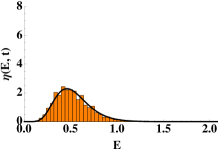
(b) $t=1000$

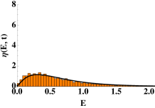
(c) $t=5000$

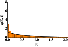
(d) $t=15000$

Figure 3: Energy distribution $\eta(E,t)$ of $10^{5}$ particles following the exact Fermi-Ulam dynamics with small wall oscillation amplitude $a=10^{-5}$ at times $t=100,~{}1000,~{}5000,$ and $15000$. The histograms are generated from numerical simulations, and the smooth curve is the analytical solution Eq. (63) for the energy distribution of a particle ensemble in the corresponding quivering billiard.

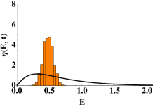
(a) $a=10^{-1}$

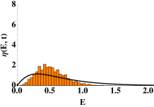
(b) $a=10^{-2}$

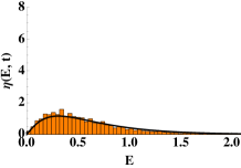
(c) $a=10^{-3}$

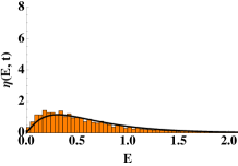
(d) $a=10^{-4}$

Figure 4: Energy distribution $\eta(E,t)$ at $t=5000$ of $10^{5}$ particles following the exact Fermi-Ulam dynamics for successively smaller wall oscillation amplitudes $a$. The histograms are generated from numerical simulations, and the smooth curve is the analytical solution Eq. (63) for the energy distribution of a particle ensemble in the corresponding quivering billiard. The case for $a=10^{-5}$ is shown in the $t=5000$ plot in Fig. 3

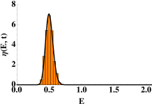
(a) $t=100$

(b) $t=1000$

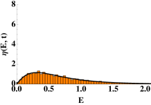
(c) $t=5000$

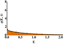
(d) $t=15000$

Figure 5: Energy distribution $\eta(E,t)$ of $10^{5}$ particles at $t=100,~{}1000,~{}5000,$ and $15000$ in a quivering billiard corresponding to the quivering limit of the Femi-Ulam model used in Fig. 3. The histograms are generated from numerical simulations, and the smooth curve is the analytical solution for the energy distribution given by Eq. (63).

The quivering limit of the Fermi-Ulam model given in Eqs. (70) and (71) is found by following the procedures described in Sec. II. We first obtain the unbiased distribution,

$$P(u_{b}|0)=\frac{1}{2}\delta(u_{b}-4u_{c})+\frac{1}{2}\delta(u_{b}+4u_{c}),$$ (72)

and then the biased distribution $P(u_{b}|v_{b-1})$,

$$P(u_{b}|v_{b-1})=\begin{cases}\frac{1}{2}\left(1-\frac{u_{b}}{v_{b-1}}\right)\left[\delta(u_{b}-4u_{c})+\delta(u_{b}+4u_{c})\right],&v_{b-1}>4u_{c}\\ \delta(u_{b}+4u_{c}),&v_{b-1}\leq 4u_{c}.\end{cases}$$ (73)

The drift and diffusion terms corresponding to this quivering billiard are found by following the procedures Sec. III.4. We note that $M_{2}(\mathbf{q}_{b})=16u_{c}^{2}$ for the moving wall, and $M_{2}(\mathbf{q}_{b})=0$ for the stationary wall, so Eq. (45) yields $\overline{u^{2}}=(1/2)~{}16u_{c}^{2}$. The coarse grained free flight distance is given simply by $\overline{l}=L$, so we find

$$g_{1}(E) = \frac{32\sqrt{2m}~{}u_{c}^{2}}{L}E^{\frac{1}{2}}=\alpha E^{\frac{1}{2}}$$ (74)

$$g_{2}(E) = \frac{64\sqrt{2m}~{}u_{c}^{2}}{L}E^{\frac{3}{2}}=2\alpha E^{\frac{3}{2}}.$$

The drift and diffusion terms are independent of time, so the rescaled time $s$ is simply $s=\alpha t$. Using the same values for $L$, $m$, and $u_{c}$ the we used in the Fermi-Ulam simulation, we find $\alpha\approx 4.53\times 10^{-5}$. Figure 5 shows the evolving energy distribution in the simulated quivering billiard, with the analytical result predicted by Eq. (63) superimposed. Our analytical solution agrees very well with the numerical simulation.

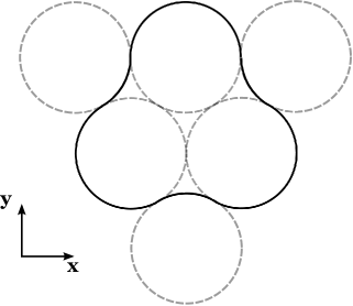
Figure 6: The six-circle clover billiard, constructed from sections of six adjacent equi-radii circles.

For pedagogical purposes, we now construct and simulate a two-dimensional quivering billiard. For the billiard shape, we have chosen the six-circle clover introduced in Ref. Jarzynski (1993), depicted here in Fig. 6. We set the normal wall velocities along the billiard boundary to be,

$$u(\mathbf{q},t)=\begin{cases}u_{c}|\hat{\mathbf{n}}(\mathbf{q})\cdot\hat{\mathbf{x}}|,&0\leq~{}\Psi(t)<\frac{1}{2}\\ -u_{c}|\hat{\mathbf{n}}(\mathbf{q})\cdot\hat{\mathbf{x}}|,&\frac{1}{2}\leq~{}\Psi(t)<1,\end{cases}$$ (75)

where $\hat{\mathbf{n}}(\mathbf{q})$ is the outward unit normal to the wall at $\mathbf{q}$ and $\hat{\mathbf{x}}$ is the unit vector in the x-direction. This choice of wall velocities gives in the quivering limit,

$$P(u_{b}|0,\mathbf{q}_{b})=\frac{1}{2}\delta\boldsymbol{(}u_{b}-u_{c}|\hat{\mathbf{n}}(\mathbf{q}_{b})\cdot\hat{\mathbf{x}}|\boldsymbol{)}+\frac{1}{2}\delta\boldsymbol{(}u_{b}+u_{c}|\hat{\mathbf{n}}(\mathbf{q}_{b})\cdot\hat{\mathbf{x}}|\boldsymbol{)}$$ (76)

$$P(u_{b}|v_{b-1},\mathbf{q}_{b},\theta_{b})=\begin{cases}\left(1-\frac{u_{b}}{v_{b-1\sin(\theta_{b})}}\right)P(u_{b}|0,\mathbf{q}_{b}),&v_{b-1}>u_{c}|\hat{\mathbf{n}}(\mathbf{q}_{b})\cdot\hat{\mathbf{x}}|\\ \delta\boldsymbol{(}u_{b}+u_{c}|\hat{\mathbf{n}}(\mathbf{q}_{b})\cdot\hat{\mathbf{x}}|\boldsymbol{)},&v_{b-1}\leq u_{c}|\hat{\mathbf{n}}(\mathbf{q}_{b})\cdot\hat{\mathbf{x}}|.\end{cases}$$ (77)

The six-circle clover constructed from equi-radii circles is fully chaotic Jarzynski (1993), so over time scales greater than the clover’s ergodic time scale, $\overline{u^{2}}$ is just $M_{2}(\mathbf{q})$ averaged uniformly over the billiard boundary. For any $\mathbf{q}$ on the boundary, we have $M_{2}(\mathbf{q})=u_{c}^{2}~{}|\hat{\mathbf{n}}(\mathbf{q})\cdot\hat{\mathbf{x}}|^{2}$, and from Fig. 6, we see the outward normals $\hat{\mathbf{n}}(\mathbf{q})$ are distributed uniformly around a unit circle, so we have $\overline{u^{2}}=(1/2)~{}u_{c}^{2}$. The coarse grained free flight distance $\overline{l}$, over time scales greater than the ergodic time scale, is just the billiard’s mean free path. For a two dimensional ergodic billiard, the mean free path is given by $\pi A/S$, where $A$ is the billiard’s area and $S$ is the billiard’s perimeter Jarzynski (1993). If the radius of the circles used to construct the six-circle clover is $R$, then the geometry of Fig. 6 gives $A=R^{2}(4\sqrt{3}+\pi)$ and $S=4\pi R$. We thus have for the drift and diffusion coefficients,

$$g_{1}(E) = \frac{2\sqrt{2m}~{}u_{c}^{2}}{l}E^{\frac{1}{2}}=\alpha E^{\frac{1}{2}}$$ (78)

$$g_{2}(E) = \frac{8\sqrt{2m}~{}u_{c}^{2}}{3~{}l}E^{\frac{3}{2}}=\frac{4}{3}\alpha E^{\frac{3}{2}}.$$

where $l=R(\sqrt{3}+\pi/4)$ is the mean free path.
Figure 7 shows the energy evolution of a microcanonical ensemble of $10^{5}$ particles in a quivering clover, with the distribution Eq. (63) superimposed. The particles have mass $m=1$ and initial energy $E_{0}=1/2$. We constructed the clover with circles of radius $R=1$ and set $u_{c}=6.35\times 10^{-3}$ to give $\alpha\approx 4.53\times 10^{-5}$. Again, we see good agreement between the distribution predicted by Eq. (63) and the simulated energy distribution.

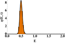
(a) $t=100$

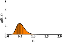
(b) $t=1000$

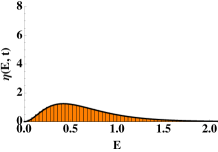
(c) $t=5000$

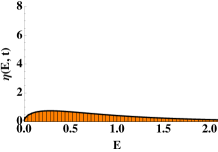
(d) $t=15000$

Figure 7: Energy distribution $\eta(E,t)$ of $10^{5}$ particles at $t=100,~{}1000,~{}5000,$ and $15000$ in a two-dimensional chaotic quivering billiard. The histograms are generated from numerical simulations, and the smooth curve is the analytical solution for the energy distribution given by Eq. (63).

VI Summary and Conclusions

In this work, we have defined a particular fixed wall limit of time-dependent billiards, the quivering limit, and explored the evolution of particles and ensembles in the resulting quivering billiards. We have conjectured that any physically consistent, non-trivial, fixed wall limit of a time-dependent billiard must be physically equivalent to the quivering limit, and we have shown that the simplifications allowed by a physically consistent fixed wall limit come at a price: deterministic billiard dynamics become inherently stochastic. Although quivering is an idealized limit of billiard motion, we have shown that for smaller and smaller oscillation amplitudes and periods, time-dependent billiards become better and better approximated by quivering billiards. Billiards that quiver or approximately quiver behave universally; particle energy evolves diffusively, particle ensembles achieve a universal asymptotic energy distribution, and quadratic Fermi acceleration always occurs, regardless of a billiard’s dimensionality or frozen dynamics. The mechanism for this quadratic Fermi acceleration is analogous to a resistive friction-like force, present due to the fluctuations induced by the erratic wall motion, as described by the fluctuation-dissipation relation in Eq. (54).
Through this work, we have gained some insight into issues that have been discussed in the previous literature. Namely, we concluded that in the quivering limit, the quasilinear approximation is exact, not an approximation. Also, we showed that the often used static wall approximation fails because it is unphysical and can not take into account the statistical bias towards inward moving wall collisions. Energy gain in the static wall approximation is a purely mixing effect; unbiased fluctuations in particle velocity produce an average increase in particle velocity squared, analogous to a Brownian random walk where unbiased fluctuations in position produce an average increase in squared distance from the initial position. From this observation, and the fact that the static wall approximation gives one half the asymptotic energy growth rate observed in exact systems, we conclude that in the quivering limit, half of the average energy gain observed in a time-dependent billiard is due to the mere presence of fluctuations, and half is due to the fact that energy gaining fluctuations are more likely than energy losing fluctuations.
We close by acknowledging that we have not given a rigorous mathematical proof showing that deterministic time-dependent billiards become stochastic quivering billiards in the quivering limit. One possible approach toward such a proof would be to define some sort of space of time-dependent billiards consisting of systems with different oscillation amplitudes and periods, define a metric to give some notion of distance in this space, and prove that particular sequences in this space with successively smaller amplitudes and periods are Cauchy sequences. One could then determine what properties the space of systems would need to posses in order to assure that these Cauchy sequences converge to limits, and then study the limits by studying the sequences that converge to them. Instead of a rigorous mathematical approach, we have taken a more intuitive approach and have attempted to justify our work by using physical reasoning and by showing consistency with previous results. We hope that the evidence is convincing enough to mitigate our mathematical deficiencies.

*

Appendix A

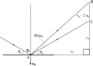
Figure 8: Incoming and outgoing particle trajectories at the $b^{th}$ collision location $\mathbf{q}_{b}$ in the full and frozen dynamics, assuming a collision wall velocity $u_{b}$. The full dynamics trajectory is perturbed by an angle $\delta\theta|u_{b}$ relative to the frozen dynamics trajectory. $\mathbf{n}_{b}$ is the outward normal to the boundary at $\mathbf{q}_{b}$.

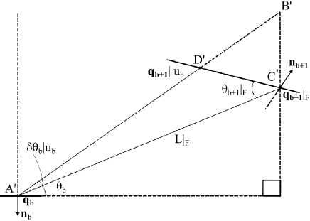
Figure 9: The geometrical relationship between $\mathbf{q}_{b}$, $\mathbf{q}_{b+1}|_{F}$, and $\mathbf{q}_{b+1}|u_{b}$. $\mathbf{q}_{b}$ and $\mathbf{q}_{b+1}|_{F}$ denote the $b^{th}$ and $(b+1)^{th}$ collision locations in the frozen dynamics, respectively, while $\mathbf{q}_{b+1}|u_{b}$ denotes the $(b+1)^{th}$ collision location in the full dynamics. $\mathbf{n}_{b}$ and $\mathbf{n}_{b+1}$ are the outward normals to the boundary at $\mathbf{q}_{b}$ and $\mathbf{q}_{b+1}|_{F}$, respectively.

Here, we find $\|\delta\mathbf{q}_{b+1}|u_{b}\|$, the magnitude of the perturbation to the frozen dynamics $(b+1)^{th}$ collision location due to the energy gained or lost at the $b^{th}$ collision in the full dynamics. In the frozen dynamics, the collision angle $\theta_{b}$ is equal to the angle of reflection. Let $\theta_{b}+\delta\theta|u_{b}$ be the reflected angle in the full dynamics, assuming a wall velocity of $u_{b}$ at the $b^{th}$ collision. We denote $v_{b-1}$ as the incoming particle speed at the $b^{th}$ collision, $v_{T}$ as the velocity component tangent to the wall, $v_{P}$ as the reflected particle’s velocity component perpendicular to the wall in the frozen dynamics, and $v_{P}|u_{b}$ as the reflected perpendicular velocity component in the full dynamics. The collision kinematics give $v_{P}|u_{b}=v_{P}-2u_{b}$. The perturbation $\delta\theta|u_{b}$ can be found using the geometry in Fig. 8. Note that $\tan(\theta_{b})=\frac{v_{P}}{v_{T}}$ and $\tan(\theta_{b}+\delta\theta|u_{b})=\frac{v_{P}|u_{b}}{v_{T}}$. Expanding $\tan(\theta_{b}+\delta\theta|u_{b})$ to first order in $\delta\theta|u_{b}$, we find

$$\tan(\theta_{b}+\delta\theta|u_{b}) = \frac{v_{P}|u_{b}}{v_{T}}$$

$$= \tan(\theta_{b})+\frac{1}{\cos^{2}(\theta_{b})}\delta\theta|u_{b}$$

$$= \frac{v_{P}}{v_{T}}+\frac{1}{\cos^{2}(\theta_{b})}\delta\theta|u_{b}.$$

Noting that $v_{P}|u_{b}=v_{P}-2u_{b}$ and $v_{T}=v_{b-1}\cos{\theta_{b}}$, we solve for $\delta\theta|u_{b}$ to find

$$\delta\theta|u_{b}=2\cos(\theta_{b})\frac{u_{b}}{v_{b-1}}.$$ (80)

Figure 9 shows the geometry of the $b^{th}$ and $(b+1)^{th}$ collisions in both the full and frozen dynamics, where $\|\delta\mathbf{q}_{b+1}|u_{b}\|$ is the length of the line segment $C^{\prime}D^{\prime}$. We assume that $\delta\theta|u_{b}$ is small enough such that the wall appears flat between the frozen and full dynamics’ $(b+1)^{th}$ collision locations. The triangle $A^{\prime}B^{\prime}C^{\prime}$ in Fig. 9 is similar to the triangle $ABC$ in Fig. 8, so we have $\frac{|BC|}{|AC|}=\frac{|B^{\prime}C^{\prime}|}{|A^{\prime}C^{\prime}|}=\frac{2|u_{b}|}{v_{b-1}}$. We note that $|A^{\prime}C^{\prime}|$ is the distance between the $b^{th}$ and $(b+1)^{th}$ collision locations in the frozen dynamics, so we denote $|A^{\prime}C^{\prime}|=L_{b}|_{F}$ and find

$$|B^{\prime}C^{\prime}|=\frac{2|u_{b}|}{v_{b-1}}L_{b}|_{F}.$$ (81)

All angles in Fig. 8 can be found in terms of $\theta_{b}$, $\theta_{b+1}|_{F}$, and $\delta\theta|u_{b}$. By applying the Law of Sines to the triangle $B^{\prime}C^{\prime}D^{\prime}$, we find

$$|C^{\prime}D^{\prime}|=2L_{b}|_{F}\frac{\cos(\theta_{b})}{\sin(\theta_{b+1}|_{F})}\frac{|u_{b}|}{v_{b-1}}.$$ (82)

We thus have

$$\|\delta\mathbf{q}_{b+1}|u_{b}\|=2L_{b}|_{F}\frac{\cos(\theta_{b})}{\sin(\theta_{b+1}|_{F})}\frac{|u_{b}|}{v_{b-1}}.$$ (83)

References

- Ott (2002) E. Ott, Chaos in Dynamical Systems (Cambridge University Press, Cambridge, England, 2002).
- Brahic (1970) A. Brahic, Astron. and Astrophys. 12, 98 (1970).
- Lieberman and Lichtenberg (1972) M. A. Lieberman and A. J. Lichtenberg, Phys. Rev. A 5, 1852 (1972).
- Lichtenberg et al. (1980) A. J. Lichtenberg, M. A. Lieberman, and R. H. Cohen, Physica D 1, 291 (1980).
- Jarzynski and Swiatecki (1993) C. Jarzynski and W. J. Swiatecki, Nucl. Phys. A552, 1 (1993).
- Fermi (1949) E. Fermi, Phys. Rev. 75, 1169 (1949).
- Zaslavskii and Chirikov (1965) G. M. Zaslavskii and B. V. Chirikov, Sov. Phys. Dokl. 9, 989 (1965).
- Ulam (1961) S. M. Ulam, in Proceedings of the Fourth Berkeley Symposium on Mathematical Statistics and Probability, Vol. 3 (California University Press, Berkeley, 1961) p. 315.
- Hammersley (1961) J. M. Hammersley, in Proceedings of the Fourth Berkeley Symposium on Mathematical Statistics and Probability, Vol. 3 (California University Press, Berkeley, 1961) p. 79.
- Gelfriech et al. (2012) V. Gelfriech, V. Rom-Kedar, and D. Turaev, Chaos 22, 033116 (2012).
- Batistic (2014a) B. Batistic, Phys. Rev. E 89, 022912 (2014a).
- Batistic (2014b) B. Batistic, Phys. Rev. E 90, 032909 (2014b).
- Wilkinson (1990) M. Wilkinson, J. Phys. A 23, 3603 (1990).
- Jarzynski (1993) C. Jarzynski, Phys. Rev. E 48, 4340 (1993).
- Karlis et al. (2008) A. K. Karlis, F. K. Diakonos, V. Constantoudis, and P. Schmelcher, Phys. Rev. E 78, 046213 (2008).
- Jarzynski (1992) C. Jarzynski, Phys. Rev. A 46, 7498 (1992).
- Revesz (1968) P. Revesz, The Laws of Large Numbers (Academic Press, 1968).
- Kargovsky et al. (2013) A. V. Kargovsky, E. I. Anashkina, O. A. Chichigina, and A. K. Krasnova, Phys. Rev. E 87, 042133 (2013).
- Loskutov et al. (2000) A. Loskutov, A. B. Ryabov, and L. G. Akinshin, J. Phys A 33, 7973 (2000).
- Khamporst and de Carvalho (1999) S. O. Khamporst and S. P. de Carvalho, Nonlinearity 12, 1363 (1999).
- Lenz et al. (2011) F. Lenz, C. Petri, F. R. N. Koch, F. K. Diakonos, and P. Schmelcher, New J. Phys 11, 083035 (2011).
- Shah (2011) K. Shah, Phys. Rev. E 83, 046215 (2011).
- Shah et al. (2010) K. Shah, D. Turaev, and V. Rom-Kedar, Phys. Rev. E 81, 056205 (2010).
- Gelfreich et al. (2011) V. Gelfreich, V. Rom-Kedar, K. Shah, and D. Turaev, Phys. Rev. Lett. 106, 074101 (2011).
- Gelfreich et al. (2014) V. Gelfreich, V. Rom-Kedar, and D. Turaev, J. Phys. A 47, 395101 (2014).
- Loskutov et al. (1999) A. Loskutov, A. B. Ryabov, and L. G. Akinshin, J. Exp. Theor. Phys. 89, 966 (1999).
- Leonel et al. (2004) E. D. Leonel, P. V. E. McClintock, and J. K. da Silva, Phys. Rev. Lett. 93, 014101 (2004).
- Karlis et al. (2006) A. K. Karlis, P. K. Papachristou, F. K. Diakonos, V. Constantoudis, and P. Schmelcher, Phys. Rev. Lett. 97, 194102 (2006).
- Karlis et al. (2007) A. K. Karlis, P. K. Papachristou, F. K. Diakonos, V. Constantoudis, and P. Schmelcher, Phys. Rev. E 76, 016214 (2007).