OU-HET-870

Band spectrum is D-brane

Koji Hashimoto¹ and Taro Kimura²

¹Department of Physics, Osaka University, Toyonaka, Osaka 560-0043, Japan
²Department of Physics, Keio University, Kanagawa 223-8521, Japan

We show that band spectrum of topological insulators can be identified as the shape of D-branes in string theory. The identification is based on a relation between the Berry connection associated with the band structure and the ADHM/Nahm construction of solitons whose geometric realization is available with D-branes. We also show that chiral and helical edge states are identified as D-branes representing a noncommutative monopole.

1 Introduction

Topological insulators and superconductors are one of the most interesting materials in which theoretical and experimental progress have been intertwined each other. In particular, the classification of topological phases [1, 2] provided concrete and rigorous argument on stability and possibility of topological insulators and superconductors. The key to find the topological materials is their electron band structure. The existence of gapless edge states appearing at spatial boundaries of the material signals the topological property. Identification of possible electron band structures is directly related to the topological nature of the topological insulators. It is important, among many possible applications of the topological insulators, to gain insight on what kind of electron band structure is possible for topological insulators with fixed topological charges.

D-branes in superstring theory [3, 4, 5] are extended objects in higher spatial dimensions which play crucial roles in any string theory dynamics. The shape of D-branes encodes information of the higher dimensions as well as non-perturbative dynamics of gauge theories living on the D-branes. In particular, D-branes have Ramond-Ramond charges which can be seen as topological charges on the brane worldvolume theories. The D-brane charges are classified by K-theory [6], which offers a natural path to relate the topological insulators and superstring theory. Indeed, recent progress [7, 8, 9] realizes a field theory setups of the topological insulators in terms of worldvolume gauge theories on D-branes, which provides a consistent K-theory interpretation with Refs. [2, 10]. The established relation is partially due to the Chern-Simons term indicating the topological nature of the theory, appearing as a part of the D-brane worldvolume gauge theory.

The topological nature of the topological insulators is, on the other hand, naturally understood in terms of electron band structure. The quantum Hall effect, which is the most popular example of the topological material, has the topological number called Thouless-Kohmoto-Nightingale-den Nijs (TKNN) number [11]. The topological number $\nu_{\rm TKNN}$ is defined as a first Chern class of the Berry connection of Bloch wave functions in the momentum space. The electron band structure crucially determines the Chern number, and the topological nature is hidden in the band spectrum.

In this paper, we show that the electron band structure of topological insulators can be identified as the shape of D-branes in string theory. The dispersion relation in the momentum space for electrons in the continuum limit is shown to be identical to the shape of a particular species of D-branes in higher dimensional coordinate space.

To relate these, we notice the following analogy between (i) the D-branes, (ii) topological solitons and (iii) the topological insulators.

• (i) $\leftrightarrow$ (ii). Particular set of D-branes in string theory can represent topological solitons of gauge theories [12, 13, 14]. Monopoles can be given by a D1-brane stuck to D3-branes as seen from the D3-brane worldvolume theory. The D3-brane exhibits a particular spiky shape in higher dimensional space. Instantons can be given by a D0-brane bound inside a pile of D4-branes.

• (ii) $\leftrightarrow$ (iii). For important kinds of topological solitons, there exists a construction method of all possible solitons. For monopoles and instantons, we have Nahm construction of monopoles [15] and Atiyah-Drinfeld-Hitchin-Manin (ADHM) construction of instantons [16, 17]. The way they work is quite analogous to the Berry connections in topological insulators.

We fully use these correspondence to find that the shape of D-branes in coordinate spaces can be identical to the shape of the electron bands in topological insulators in momentum space.

In [18], the stability of the Fermi surfaces was topologically studied from the viewpoint of K-theory, and possible relation to D-branes due to the K-theory was pointed out, through the exchange of the coordinate space and the momentum space. See also [19] and [20]. Based on this exchange, we find an explicit and new connection between the electron bands and the shape of the D-branes.

We first study typical examples of class A topological insulators both in 2 and 4 dimensions, which have no additional discrete symmetry, according to the established classification of topological phases [1, 2]. We start with a popular topological property of a Hamiltonian of a free electron, and will find that it parallels the Nahm and ADHM constructions of monopoles and instantons. Such topological solitons respect supersymmetries in string theory and are represented by a set of D-branes. To have a direct relation, we use the fact that some scalar field is associated with the topological solitons, through Bogomol’nyi-Prasad-Sommerfield (BPS) equations. The scalar field configuration is the shape of D-branes, and we can show that it can be identified with the electron dispersion relation through the connection described.

In this paper we consider the following D-brane configurations: D1-branes stuck to a D3-brane, and a D0-brane within D4-branes with fundamental strings stuck to them, and a D1-brane piercing a D3-brane at an oblique angle (see Fig. 1). Through (i) $\leftrightarrow$ (ii), each brane setup corresponds respectively to $U(1)$ monopoles, dyonic instantons [21] and a monopole in non-commutative space [22, 23, 24, 25]. Then, through (ii) $\leftrightarrow$ (iii), each corresponds respectively to 2-dimensional and 4-dimensional class A topological insulators, and a chiral edge state at the boundary of the 2-dimensional topological insulators. In each example, we find that the D-brane shape is the electron band structure.

This argument can be generalized to other classes by applying discrete symmetry. We in particular study the class AII system by imposing time-reversal symmetry, and show how the helical edge state, which is peculiar to this case, can be understood from the string theoretical point of view. The symmetry applied here can be realized by using an orientifold, and we show how it stabilizes the D-brane configuration corresponding to the helical edge state.

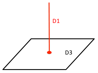
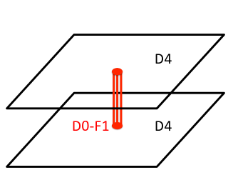
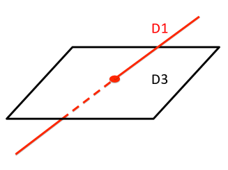
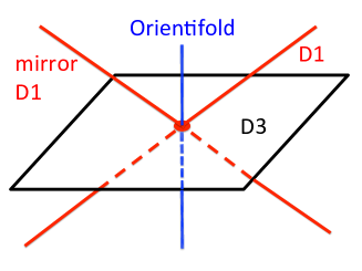
Figure 1: Top-Left: a D1-brane stuck to a D3-brane, corresponding to a $U(1)$ monopole, and to an electron band of the 2-dimensional topological insulator. Top-Right: a D0-F1(fundamental string) bound state stuck to two parallel D4-branes, corresponding to a dyonic instanton, and to a band structure of the 4-dimensional topological insulator. Bottom-Left: a D1-brane piercing a D3-brane at an oblique angle, corresponding to an energy dispersion of a chiral edge state at the boundary of the 2-dimensional class A topological insulator. Bottom-Right: An orientifold makes a mirror image of the slanted D1-brane, corresponding to an energy dispersion of a helical edge state at the boundary of the 2-dimensional class AII topological insulator.

The merit of presenting a map between the band structure of electrons and the shape of D-branes is to have a better understanding of possible band structure, as D-branes have fertile and fruitful applications in string theory in higher dimensions. In this paper, we partially identify the mechanism of how topological insulators can acquire a topological number larger than 1 for class A systems. We solve the constraint equation of the soliton construction techniques, which are called the Nahm equation, to find a class of electron Hamiltonians which have larger and generic topological numbers, and discuss its realization in a multilayer system.

The organization of this paper is as follows. In section 2, we study the 2-dimensional class A topological insulators. We briefly review the Nahm construction of monopoles, and study its relevance to the Hamiltonian, Berry connection and the topological number. Then we identify the shape of the deformed D3-branes as the electron dispersion relation. We study how larger topological numbers are realized in Hamiltonians, through the shape of the D-branes. In section 3, we further generalize the correspondence to the 4-dimensional class A topological insulators. We will find that the D-brane shape is related to the electron dispersion through the dyonic instanton which probes the shape of the instanton through the additional scalar field. In section 4, we turn to a boundary of the 2-dimensional topological insulators. There, the electron Hamiltonian is identified with the Nahm construction in a noncommutative space. The solutions of noncommutative monopoles are represented by a slanted D1-brane which is shown to relate directly to the shape of the dispersion relation of the chiral edge state. In section 5, we generalize this argument to the class AII system in 2 dimensions by imposing time-reversal symmetry. We show that this symmetry is realized by using an orientifold for the D-brane configuration. It naturally requires a mirror D1-brane which is allowed to intersect with the orientifold as a pair. This pair of D1-branes exhibits the helical edge state in the class AII topological insulator. The final section is for a summary and discussions for further applications.

2 2D class A and D1-D3 brane systems

In this section, we show that a band spectrum of a 2 dimensional class A topological insulator is identified as the shape of a D-brane.

2.1 A brief review of Nahm construction of monopoles

Our identification of the band and the D-brane is based on Nahm construction of monopoles  [15]. It is a complete process to construct all solutions of BPS equations for monopoles. In particular, it is useful for constructing multiple monopole solutions in non-Abelian gauge theories, but here for our purpose a single monopole in Abelian gauge theory suffices. We shall give a brief review of how it is constructed.

First we prepare for a “Dirac operator” $\nabla^{\dagger}$ in one dimension parameterized by a coordinate $\xi$,

$$\nabla^{\dagger}\equiv i\frac{d}{d\xi}+i\sigma_{i}\left(x^{i}-T_{i}(\xi)\right)\,.$$ (2.1)

Here $\sigma_{i}(i=1,2,3)$ is the Pauli matrix, and $T_{i}(\xi)$ is a $k\times k$ Hermitian matrix which satisfies the Nahm equation,

$$\frac{d}{d\xi}T_{i}=i\epsilon_{ijk}T_{j}T_{k}\,.$$ (2.2)

The matrix size $k$ is for $k$ monopoles. For example, for a single monopole $k=1$, the Nahm equation is trivially solved by $T_{i}(\xi)=0$.

Next, we solve the “Dirac equation”

$$\nabla^{\dagger}v(\xi)=0$$ (2.3)

where the vector $v(\xi)$ is normalized as

$$\int_{-\infty}^{0}d\xi\;v^{\dagger}v=1.$$ (2.4)

This expression is for $U(1)$ BPS monopoles.

Finally, the monopole solution satisfying a $U(1)$ BPS equation

$$\partial_{i}\Phi(x)=\frac{1}{2}\epsilon_{ijk}F_{jk}(x)$$ (2.5)

is given by

$$\Phi(x)\equiv\int\!d\xi\;v^{\dagger}\xi v\,,\quad A_{i}(x)\equiv\int\!d\xi\;v^{\dagger}i\frac{d}{dx^{i}}v\,,$$ (2.6)

where $\Phi$ and $A_{i}(i=1,2,3)$ are Hermitian.

As an exercise, using the Nahm construction let us construct a BPS $U(1)$ Dirac monopole solution

$$\Phi(x)=\frac{-1}{2r}\,,\quad B_{i}\left(=\frac{1}{2}\epsilon_{ijk}F_{jk}\right)=\frac{x^{i}}{2r^{3}}\,,$$ (2.7)

where $r\equiv\sqrt{(x^{1})^{2}+(x^{2})^{2}+(x^{3})^{2}}$. The normalized zero mode solving the “Dirac equation” (2.3) is easily obtained as

$$v=\frac{1}{\sqrt{r+x^{3}}}\exp(r\xi)\;\left(\begin{array}[]{c}-x^{1}+ix^{2}\\ r+x^{3}\end{array}\right)\,.$$ (2.10)

Then using the formulas (2.6), we obtain the BPS Dirac monopole solution (2.7). The Dirac string is at the negative axis of $x^{3}$, as seen from the vector (2.10) having an ill-defined normalization factor there.

As for our later purpose let us construct $k=2$ monopole solution. The Nahm equation (2.2) can be solved by

$$T_{1}=\Delta\sigma_{1},\;T_{2}=T_{3}=0$$ (2.11)

where $\Delta$ is a constant parameter. With this, the “Dirac equation” (2.3) is given by

$$\frac{d}{d\xi}v+\left(\begin{array}[]{cccc}x^{3}&x^{1}-ix^{2}&&\Delta\\ x^{1}+ix^{2}&-x^{3}&\Delta&\\ &\Delta&x^{3}&x^{1}-ix^{2}\\ \Delta&&x^{1}+ix^{2}&-x^{3}\end{array}\right)v=0.$$ (2.16)

The solutions are

$$v_{-}=\frac{\exp[r_{-}\xi]}{\sqrt{2(x^{3}+r_{-})}}\left(\begin{array}[]{c}x^{1}-ix^{2}-\Delta\\ -(x^{3}+r_{-})\\ -(x^{1}-ix^{2}-\Delta)\\ x^{3}+r_{-}\end{array}\right),\quad v_{+}=\frac{\exp[r_{+}\xi]}{\sqrt{2(x^{3}+r_{+})}}\left(\begin{array}[]{c}x^{1}-ix^{2}+\Delta\\ -(x^{3}+r_{+})\\ x^{1}-ix^{2}+\Delta\\ -(x^{3}+r_{+})\end{array}\right),$$ (2.25)

(2.26)

where $r_{\pm}\equiv\sqrt{(x^{1}\pm\Delta)^{2}+(x^{2})^{2}+(x^{3})^{2}}$. These vectors are orthogonal to each other and normalized. The scalar field is obtained by the Nahm construction formula as

$$\Phi=\int_{-\infty}^{0}d\xi\left(v_{-}^{\dagger}\xi v_{-}+v_{+}^{\dagger}\xi v_{+}\right)=\frac{-1}{2r_{-}}+\frac{-1}{2r_{+}}\,.$$ (2.27)

We find that two $U(1)$ monopoles are located at $(x^{1},x^{2},x^{3})=(\pm\Delta,0,0)$, and the monopole charge is two. The Dirac strings are in the negative $x^{3}$ direction emanating from each monopole.

2.2 The shape of D-brane relates to electron band structure

We start with the model Hamiltonian in 2 dimensions, describing the vicinity of the band crossing point,

$${\cal H}=\sigma_{1}p_{1}+\sigma_{2}p_{2}+\sigma_{3}m$$ (2.28)

where $p_{1},p_{2}$ are momentum of the electron and $m$ is the band gap, playing a role of the mass term. The eigenvalues of this Hamiltonian (2.28) are simply given by

$$\epsilon=\pm\sqrt{p_{1}^{2}+p_{2}^{2}+m^{2}}\,.$$ (2.29)

This is a dispersion relation of a relativistic particle with its mass $m$.

class $\backslash$ $d$	0	1	2	3	4	5	6	7	T	C	S
A	$\mathbb{Z}$	0	$\mathbb{Z}$	0	$\mathbb{Z}$	0	$\mathbb{Z}$	0	0	0	0
AIII	0	$\mathbb{Z}$	0	$\mathbb{Z}$	0	$\mathbb{Z}$	0	$\mathbb{Z}$	0	0	1
AI	$\mathbb{Z}$	0	0	0	$2\mathbb{Z}$	0	$\mathbb{Z}_{2}$	$\mathbb{Z}_{2}$	$+$	0	0
BDI	$\mathbb{Z}_{2}$	$\mathbb{Z}$	0	0	0	$2\mathbb{Z}$	0	$\mathbb{Z}_{2}$	$+$	$+$	1
D	$\mathbb{Z}_{2}$	$\mathbb{Z}_{2}$	$\mathbb{Z}$	0	0	0	$2\mathbb{Z}$	0	0	$+$	0
DIII	0	$\mathbb{Z}_{2}$	$\mathbb{Z}_{2}$	$\mathbb{Z}$	0	0	0	$2\mathbb{Z}$	$-$	$+$	1
AII	$2\mathbb{Z}$	0	$\mathbb{Z}_{2}$	$\mathbb{Z}_{2}$	$\mathbb{Z}$	0	0	0	$-$	0	0
CII	0	$2\mathbb{Z}$	0	$\mathbb{Z}_{2}$	$\mathbb{Z}_{2}$	$\mathbb{Z}$	0	0	$-$	$-$	1
C	0	0	$2\mathbb{Z}$	0	$\mathbb{Z}_{2}$	$\mathbb{Z}_{2}$	$\mathbb{Z}$	0	0	$-$	0
CI	0	0	0	$2\mathbb{Z}$	0	$\mathbb{Z}_{2}$	$\mathbb{Z}_{2}$	$\mathbb{Z}$	$+$	$-$	1

Table 1: Classification of topological insulators and topological superconductors [1, 2]. This classification is associated with discrete symmetries, time-reversal (T), particle-hole (C), and chiral (sublattice) (S) symmetries. A system classified into class A which we focus on in this part has no additional discrete symmetry. We will also discuss the class AII system by imposing time-reversal symmetry in section 5.

This system is classified into class A according to the periodic table of topological insulators [1, 2]. As summarized in Table 1, the class A system has topological charge $\mathbb{Z}$ in even dimensions, and no additional discrete symmetry. In this sense it is the most generic situation, which can be a good starting point to study. Other classes can be realized by imposing additional symmetries. In section 5, for example, we will explain how to incorporate the time-reversal symmetry. We remark that this classification is completely parallel to possible D-brane charges based on K-theory [6], and the class A corresponds to type IIA string theory having D-branes in even dimensions.

Let us point out a relevance to the “Dirac equation” (2.3) of the Nahm construction of monopoles. We find that (2.3) for a single $U(1)$ monopole is identical to the Hamiltonian time evolution

$$\left[i\frac{\partial}{\partial t}+{\cal H}\right]v(t)=0$$ (2.30)

with the Hamiltonian (2.28), when one identifies $\xi\leftrightarrow it$ and

$$(x^{1},x^{2},x^{3})\leftrightarrow(p_{1},p_{2},m).$$ (2.31)

Using the eigenvalues (2.29), the “Dirac operator” $\nabla^{\dagger}$ is written as

$$\nabla^{\dagger}\sim\frac{\partial}{\partial\xi}\pm\epsilon\,,$$ (2.32)

so the zero mode of it is proportional to $\exp[\epsilon\xi]$. This particular form of the eigenfunction, together with $\epsilon\sim\int\!d\xi\;v^{\dagger}(\partial/\partial\xi)v$, leads to a novel relation

$$\Phi=\int d\xi\;v^{\dagger}\xi v\sim\frac{1}{\epsilon}.$$ (2.33)

A precise expression between the electron energy and the scalar field of the BPS monopole via the Nahm construction is found as

$$\pm 2\epsilon=\frac{1}{\Phi}\,.$$ (2.34)

The scalar field of the BPS monopole is nothing but the shape of the D-brane: a D1-brane stuck perpendicular to a D3-brane [14]. The scalar field is a deformation of the D3-brane surface, causing a spike configuration. When identifying the electron dispersion with the shape of a D-brane, we note two points:

• The coordinate in which the D-brane lives is interpreted as the electron’s momentum and the mass, as in (2.31).

• The D-brane shape is measured in a space in which the transverse coordinate is inverse of the original flat coordinate, $X=1/\Phi$.

In particular, the latter changes the spike shape $\phi\sim 1/r$ (which would be popular in string theory) to a conic shape $\Phi\sim r$. This transformation is just one of the general coordinate transformation of the target space of string theory, and is popular for the case of $AdS$ geometries, see for example Ref. [28].

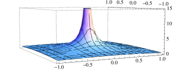
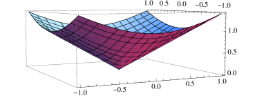
Figure 2: Left: a spike configuration representing a D1-brane stuck to a D3-brane. The D1-brane can be seen as a monopole from the D3-brane gauge theory. Right: the same configuration in a different coordinate $X=1/\Phi$. The coordinate in the vertical direction is replaced by its inverse.

In Fig. 2, we plot a spike configuration of the D1-D3 brane system, in the two ways, for $m=0$. The conic shape is in the coordinate $X=1/\Phi$ for the direction transverse to the D3-brane. We can see the Dirac cone for a massless particle.

The agreement is not a coincidence. It is known that the free relativistic electron with mass $m$ given by the Hamiltonian (2.28) is characterized by a topological number, the TKNN number [11]. The TKNN number is defined as follows. First, we consider an eigenstate of the Hamiltonian (2.28),

$${\cal H}(p_{1},p_{2},m)\;v=\epsilon\;v\,$$ (2.35)

which needs to be normalized, $v^{\dagger}v=1$. Using this eigenstate $v$, we define a Berry connection

$$A_{\mu}^{\rm(B)}=v^{\dagger}i\frac{d}{dp_{\mu}}v\;(\mu=1,2)$$ (2.36)

Then this connection exhibits a topological property; the field strength defined by the Berry phase shows half-integer quantization

$$\frac{1}{2\pi}\int\!dp_{1}dp_{2}\;F_{12}^{\rm(B)}=\frac{1}{2}\text{sign}(m)\,.$$ (2.37)

In particular, taking a difference for positive and negative $m$, we obtain the integral topological number

$$\nu \equiv \frac{1}{2\pi}\int\!dp_{1}dp_{2}\;F_{12}^{\rm(B)}(m>0)-\frac{1}{2\pi}\int\!dp_{1}dp_{2}\;F_{12}^{\rm(B)}(m<0)$$ (2.38)

$$= 1\,.$$

At this stage we find a complete analogy with the Nahm construction of monopoles. The Berry connection (2.36) is almost identical to the formula for the gauge field in the Nahm construction of monopoles (2.6). The difference is just the integral over $\xi$, which can be shown to be irrelevant for the present case, due to the form of the eigenfunction $\exp[r\xi]$.

Note that the space in which the monopole lives is $(p_{1},p_{2},m)$. Then the total monopole charge calculated by integrating the magnetic flux surrounding the monopole located at the origin is

$$1=\frac{1}{2\pi}\int\!d{\bf S}\cdot{\bf B}=\frac{1}{2\pi}\int\!dp_{1}dp_{2}\;F_{12}\biggm{|}_{m>0}-\frac{1}{2\pi}\int\!dp_{1}dp_{2}\;F_{12}\biggm{|}_{m<0}\,.$$ (2.39)

This is nothing but the calculation of the topological number (2.38). So, we find that the monopole charge due to the Nahm construction parallels the topological charge of the class A system. Along the course, the band is identified with the shape of the D-brane.

2.3 Generalization to topological number $\nu=2$

2.3.1 Copies of electrons for higher topological numbers

The topological number calculated in the previous subsection is for $\nu=1$. Generically, for the class A systems, the topological charge is a Chern class labeled by integral topological number $\mathbb{Z}$, and it should be possible to generalize it to the cases with more monopoles. Here, we use the Nahm construction to obtain a fermion system which has $\nu=2$. We generalize the correspondence between the D-brane shape and the electron dispersion to the case with $\nu=2$.

As we have seen previously, the Nahm construction of monopoles coincides with the Hamiltonian of a single free electron system. To obtain $\nu=2$ we just follow the Nahm construction to find what kind of electron system is relevant for the topological charge $\nu=2$.

We have studied the $k=2$ monopole, and what we need to do is to look at Nahm data and rephrase it to some electron Hamiltonians. First, notice that Nahm’s “Dirac operator” $\nabla^{\dagger}$ is a $2k\times 2k$ matrix for the monopole number $k$. The Nahm data $T_{i}$ are $k\times k$ matrices, which are tensored with the Pauli matrices $\sigma_{i}$. So, to have a higher topological charge, we need to prepare $k$ copies of electron Hamiltonians.

The Nahm data has to satisfy the Nahm equation (2.2). Since our extra dimension $\xi$ necessary for the Nahm construction corresponds to an auxiliary parameter for the electron case, we look at $\xi$-independent Nahm data. A generic solution to (2.2) is given by

$$T_{i}=\Delta_{i}A$$ (2.40)

where $\Delta_{i}$ $(i=1,2,3)$ is an arbitrary real constant parameter, and $A$ is an arbitrary 2 by 2 Hermitian constant matrix. A special case was studied in (2.11). The Hermitian matrix can be decomposed to a unit matrix and Pauli matrices, so

$$T_{i}=\Delta_{i}\left({\bf 1}_{2}+b_{k}\sigma_{k}\right)$$ (2.41)

where $b_{i}$ $(i=1,2,3)$ are constant real parameters.

The corresponding electron system has a Hamiltonian

$${\cal H}={\bf 1}_{2}\otimes(\sigma_{1}p_{1}+\sigma_{2}p_{2}+\sigma_{3}m)-T_{i}\otimes\sigma_{i}$$ (2.42)

The correspondence tells us that $T_{i}$ of the form (2.40) exhibits the topological charge $\nu=2$. So we are led to a conclusion that the Hamiltonian (2.42) is responsible for 2-dimensional topological insulator with topological charge $\nu=2$, once (2.40) is satisfied.

Note that the interacting Hamiltonian of the form (2.42) with (2.40) is a sufficient condition to get $\nu=2$. This is because we simply set $\xi$-independence for simplicity, and generically various monopole solutions with $\xi$-dependent Nahm data are possible.

2.3.2 The shape of D-branes and electron dispersion for $\nu=2$

Here for simplicity we shall consider the simplest Nahm data (2.11) for the $k=2$ monopole in the Nahm construction. The resultant configuration of the D3-brane consist of just two spikes whose centers are located at $x^{1}=\pm\Delta,x^{2}=x^{3}=0$. See the left figure in Fig. 3. The two spikes correspond to two D1-branes stuck to the D3-brane, and from the viewpoint of the worldvolume of the D3-brane, they are two monopoles.

Let us see a relation to the electron dispersion relation. The Hamiltonian of the electron, corresponding to (2.11), is

$${\cal H}=\left(\begin{array}[]{cccc}m&p^{1}-ip^{2}&&\Delta\\ p^{1}+ip^{2}&-m^{3}&\Delta&\\ &\Delta&m&p^{1}-ip^{2}\\ \Delta&&p^{1}+ip^{2}&-m^{3}\end{array}\right).$$ (2.47)

We find two eigenvectors corresponding to $v_{-}$ and $v_{+}$ in (2.26). The eigenvalues are

$$\epsilon_{\pm}=\sqrt{(p_{1}\pm\Delta)^{2}+(p_{2})^{2}+m^{2}}\,,$$ (2.48)

therefore the zero of the momentum $p_{1}$ is shifted by $\Delta$. Using the correspondence (2.31), we find approximately

$$2\epsilon=\frac{-1}{\Phi}$$ (2.49)

near the location of the monopoles. This expression is the same as that of the single monopole case, (2.34). Plotting $-1/\Phi$, we find two Dirac cones (see the right figure of Fig. 3).

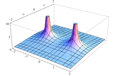
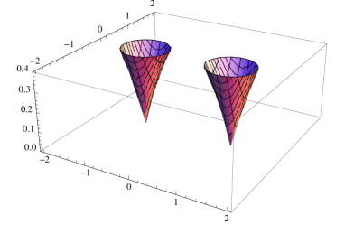
Figure 3: (Left) The shape of the D3-brane for monopole number $k=2$. The vertical axis is $-\Phi(x)$. (Right) A plot of $1/\Phi$. We find two Dirac cones.

2.3.3 Bilayer graphene and Nahm equation

For $m=0$, the Hamiltonian (2.42) includes bilayer graphene. The monopole number $k=2$, which is the topological charge, needs a twice large Hamiltonian matrix. The enlarged Hamiltonian is naturally realized by a bilayer graphene. The Nahm data term $\sigma_{i}\otimes T_{i}$ in (2.42) naturally encodes inter-layer interactions, for $b_{1},b_{2}\neq 0$.

Let us discuss briefly a correspondence to bilayer graphene (see Ref. [29] for a review of graphene). It is often convenient to describe the effective low energy Hamiltonian at the continuum as

$${\cal H}=\left(\begin{array}[]{cc}H(p)&H_{\perp}\\ (H_{\perp})^{\dagger}&H(p)\end{array}\right),\quad H(p)\equiv\left(\begin{array}[]{cc}0&p^{1}-ip^{2}\\ p^{1}+ip^{2}&0\end{array}\right),$$ (2.54)

where $H_{\perp}$ is a $2\times 2$ generic matrix responsible for the inter-layer interactions. This $H_{\perp}$ can depend on the momentum $p$, but here we consider only the case with $p$-independent constant matrix.

The first example is an AA-stacking bilayer graphene [30] which has the following inter-layer interaction

$$H_{\perp}\equiv\left(\begin{array}[]{cc}\Delta&0\\ 0&\Delta\end{array}\right).$$ (2.57)

This corresponds to the following Nahm data

$$T_{1}=\Delta{\bf 1}_{2},\quad T_{2}=T_{3}=0,$$ (2.58)

satisfying the Nahm equation (2.2). So it should naturally exhibit $\nu=2$.

On the other hand, an AB-stacking (Bernal stacking) bilayer graphene (see a review [31]) may have

$$H_{\perp}=\left(\begin{array}[]{cc}0&0\\ \Delta&0\end{array}\right)$$ (2.61)

which is not consistent with the form (2.40). Therefore our naive ansatz of having a $\xi$-independent Nahm data does not work, so we cannot make sure that it has $\nu=2$.

It would be an interesting question if the twisted graphene having typically the following effective Hamiltonian [32]

$$H_{\perp}=\Delta\left(\begin{array}[]{cc}1&1\\ 1&1\end{array}\right)+\cdots$$ (2.64)

can be in our category of Nahm data. The result should depend on whether the first term in (2.64) dominates against others.

This argument is straightforwardly generalized to multilayer graphenes. Applying the same procedure, we can similarly obtain higher topological number situations, depending on how to stack the layers.

2.4 All possible Hamiltonians for higher topological charges

Since we have shown the equivalence between the dispersion relation of the 2-dimensional topological insulators and the shape of D-branes, we would like to use the relation to discuss what are all possible Hamiltonians which have generic topological number.

The shape of D-branes has an intuitive understanding of what kind of configurations are possible. As we have seen in Fig. 3, an example of the two-monopole configuration suggests that possible configurations are only by positions of the monopoles. First, let us concentrate on the case of $k=1$ and $k=2$.

As we have learnt in this section, the eigenvalues of the Hamiltonian can either be positive or negative, and they are paired. The eigenvalues $\pm\epsilon$ corresponds to $\pm r$ in the Nahm construction. So, choosing one sign for the energy means to choose $+r$ and discard $-r$. In the Nahm construction, this in fact means that we consider only monopoles in $U(1)$ gauge theory. In order to construct non-Abelian monopoles, one needs both $+r$ and $-r$ and restrict the allowed region of $\xi$ to be a finite period. In our case, we need only the positive eigenvalues which means that we treat $U(1)$ monopoles and an Abelian Berry connection, as we assume that generic energy eigenstates are not degenerate.

For $k=1$, the generic solution of the Nahm equation (2.2) is

$$T_{i}=c_{i}$$ (2.65)

where $c_{i}$ $(i=1,2,3)$ is a constant parameter. Looking at the zero-mode equation (2.3), we see that these $c_{i}$ specify the location of the monopole, $(x^{1},x^{2},x^{3})=(c_{1},c_{2},c_{3})$. Using our dictionary (2.31), this translates to the zeros of the eigenvalues in the momentum space and the mass:

$$(p_{1},p_{2},m)=(c_{1},c_{2},c_{3})\,.$$ (2.66)

This means that for the topological charge $\nu=1$, once the BPS equation (2.5) is assumed for the application of the Nahm construction, all possible Hamiltonian is just given by a simple translation in $(p_{1},p_{2},m)$-space.

Next, let us consider the case $k=2$. Once we assume that the Nahm data is independent of $\xi$ (which may be a natural assumption since electron Hamiltonian does not depend on time $t$, since $\xi$ is interpreted as imaginary $t$), generic solution of the Nahm equation is given by (2.41), other than the total shift $(c_{i})$. Using the redundant symmetry $T_{i}\rightarrow UT_{i}U^{\dagger}$ with any unitary transformation $U\in SU(k)$, we can further bring (2.41) to a diagonal form

$$T_{i}=c_{i}{\bf 1}_{2}+d_{i}\sigma_{3}=\left(\begin{array}[]{cc}c+d&0\\ 0&c-d\end{array}\right).$$ (2.69)

So, basically, the Nahm data is the position of the two monopoles. The D-brane configuration shown in Fig. 3 turns out to be generic. Possible Hamiltonians with $\nu=2$ are parameterized only by the positions of the monopoles, once the BPS equation for monopoles (2.5) is assumed.

We can generalize this argument to arbitrary monopole charge $k$. $\xi$-independent Nahm data $T_{i}$ means that the Nahm equation reduces to

$$[T_{i},T_{j}]=0\,.$$ (2.70)

The unique solution of this equation is made by diagonal matrices,

$$T_{i}=U{\rm diag}(c_{i}^{(1)},\ldots,c_{i}^{(k)})U^{\dagger}$$ (2.71)

where $U$ is a generic $U(k)$ unitary matrix. So, generic monopole configuration consists of just arbitrary distribution of center locations of the $k$ monopoles.

This confirms that the intuitive picture of D-branes exhaust all possible Hamiltonians of 2-dimensional class A systems without any additional symmetries. Possible Hamiltonians having the nontrivial topological charge $\nu=k$ is only dictated by the location of the $k$ monopoles in the $(p_{1},p_{2},m)$-space, under the assumption that the monopoles obey the BPS equations and the electrons are free except for inter-layer momentum-independent interactions.

3 4D class A, dyonic instanton and D0-F1-D4 systems

In this section, we consider a 4-dimensional class A systems and study its relation to the shape of D-branes in string theory. According to the periodic table presented in Table 1, this system has integral topological charge $\mathbb{Z}$, and hypothetical topological insulators in 4 spatial dimensions are in fact classified by a second Chern class, e.g. 4-dimensional quantum Hall effect [33, 34]. The Chern class counts Yang-Mills instanton number, where generic solutions to self-dual equation of Yang-Mills are given by ADHM constructions [16, 17]. Furthermore, the instantons can be regarded as a D-brane bound states: D0-brane sitting and dissolved inside the worldvolume of multiple D4-branes can be seen as a Yang-Mills instanton configuration [12, 13]. The shape of the instanton can be detected again by introducing a scalar field, to form a dyonic instanton [21]. This scalar field is nothing but the shape of the D-brane corresponding to the dyonic instantons, which is known [35] to be a D0-F1-D4 bound state and supertubes [36, 37, 38] suspended between parallel D4-branes.

In the following, first we briefly review the ADHM construction of instantons, then study the shape of the corresponding D-branes to relate it to electron dispersion in 4-dimensional topological insulators.

3.1 A brief review of ADHM construction of instantons

The ADHM construction of instantons [16, 17] allows calculating all solutions of the self-dual equation of $SU(N)$ Yang-Mills theory,

$$F_{\mu\nu}=*F_{\mu\nu}$$ (3.1)

where $F_{\mu\nu}\equiv\partial_{\mu}A_{\nu}-\partial_{\nu}A_{\mu}-i[A_{\mu},A_{\nu}]$ and the Hodge dual $*$ is given by $*F_{\mu\nu}=(1/2)\epsilon_{\mu\nu\rho\sigma}F_{\rho\sigma}$ ($\mu,\nu=1,2,3,4$). The instantons are classified by the topological charge, namely the second Chern class, as

$$k=\frac{1}{16\pi^{2}}\int\!d^{4}x\;{\rm tr}\left[F_{\mu\nu}*F_{\mu\nu}\right]\,.$$ (3.2)

The ADHM procedure to obtain the solutions with the instanton number $k$ is as follows. First, we prepare “Dirac operator”

$$\nabla^{\dagger}\equiv\left(S^{\dagger}\;\;\;\bar{e}_{\mu}\otimes(x_{\mu}{\bf 1}_{k}-T_{\mu})\right)$$ (3.3)

where $T_{\mu}$ ($\mu=1,2,3,4$) is a $k\times k$ Hermitian matrix, and $S^{\dagger}$ is a $2k\times N$ complex matrix. The Pauli matrices are $e_{\mu}=(i\sigma_{1},i\sigma_{2},i\sigma_{3},{\bf 1}_{2})$ and $\bar{e}_{\mu}$ is a complex conjugate of $e_{\mu}$. The ADHM equation which the ADHM data $S$ and $T_{\mu}$ need to satisfy is

$${\rm tr}\left[\sigma_{i}\left(S^{\dagger}S+\bar{e}_{\mu}e_{\nu}T_{\mu}T_{\nu}\right)\right]=0\quad(i=1,2,3)$$ (3.4)

To construct instanton configurations, we solve the zero mode equation

$$\nabla^{\dagger}v=0$$ (3.5)

where $v$ is a vector with $N+2k$ components. Due to the size of $\nabla^{\dagger}$, there exist $N$ independent vectors, so we label them as $v^{(a)}$ $(a=1,2,\ldots,N)$. Then the gauge connection of the instanton, as a function of $x_{\mu}$, is given by

$$A_{\mu}^{ab}\equiv i\left(v^{(a)}\right)^{\dagger}\frac{d}{dx_{\mu}}v^{(b)}.$$ (3.6)

Let us demonstrate how the simplest nontrivial case works, for our later purpose. It is for $SU(2)$ Yang-Mills instanton with the instanton number $k=1$. For $k=1$, $T_{\mu}$ in the ADHM data is just constant parameters, whose meaning is just a translation of $x_{\mu}$. So we can put $T_{\mu}=0$ without losing generality. Then the ADHM equation (3.4) with generic $2\times 2$ complex matrix $S=\alpha_{\mu}e_{\mu}$ provides

$${\rm tr}\left[\sigma_{i}\bar{e}_{\mu}e_{\nu}\right]\alpha^{*}_{\mu}\alpha_{\nu}=0\,.$$ (3.7)

This condition amounts to $\alpha^{*}_{k}\alpha_{l}\epsilon_{ikl}+\alpha^{*}_{4}\alpha_{i}-\alpha^{*}_{i}\alpha_{4}=0$. A generic solution to this equation is parameterized as $S=\rho U$ where $U$ is an $U(2)$ matrix and $\rho$ is a complex constant parameter. Since this $U$ rotation does not change the final form of the gauge connection $A_{\mu}(x)$ of the instantons, we can use $U$ transformation to simplify the ADHM data. Then we can take $S=\rho{\bf 1}_{2}$ with $\rho$ being a non-negative real parameter. The “Dirac operator” for the present case is a $2\times 4$ matrix,

$$\nabla^{\dagger}=\left(\rho{\bf 1}_{2}\;\;\bar{e}_{\mu}x_{\mu}\right)\,.$$ (3.8)

The normalized zero-mode $\nabla^{\dagger}v=0$ is solved as

$$v=\frac{1}{\sqrt{r^{2}+\rho^{2}}}\left(\begin{array}[]{c}\bar{e}_{\mu}x_{\mu}\\ -\rho{\bf 1}_{2}\end{array}\right)$$ (3.11)

In this expression, two zero-modes are aligned to form a $4\times 2$ matrix $v$, and we defined $r\equiv\sqrt{x_{\mu}x_{\mu}}$ as the distance from the center of the instanton in the 4-dimensional space. Using this zero-mode, following (3.6), we can calculate the self-dual connection

$$A_{\mu}=iv^{\dagger}\frac{d}{dx_{\mu}}v\,=\frac{i}{r^{2}+\rho^{2}}\left(e_{\nu}x_{\nu}\bar{e}_{\mu}-x_{\mu}{\bf 1}_{2}\right)$$ (3.12)

With this, we can explicitly show that the field strength is self-dual,

$$F_{\mu\nu}=\frac{1}{2}\epsilon_{\mu\nu\rho\sigma}F_{\rho\sigma}=\frac{i\rho^{2}}{(r^{2}+\rho^{2})^{2}}\left(e_{\mu}\bar{e}_{\nu}-e_{\nu}\bar{e}_{\mu}\right),$$ (3.13)

and the instanton number (3.2) is $k=1$.

The parameter $\rho$ is the size of the instanton. We will use the following property later,

$$iv^{\dagger}\frac{d}{d\rho}v=0$$ (3.14)

for $v$ of this $SU(2)$ single instanton.

3.2 4-dimensional class A system and ADHM construction

Let us consider a free class A system in 4 spatial dimensions, whose Hamiltonian is provided by

$${\cal H}=\gamma_{\mu}p_{\mu}+\gamma_{5}m$$ (3.15)

where $\mu=1,2,3,4$ is for the four spatial directions, and $m$ is the mass. We have defined the gamma matrices

$$\gamma_{\mu}\equiv\left(\begin{array}[]{cc}0&\bar{e}_{\mu}\\ e_{\mu}&0\end{array}\right),\quad\gamma_{5}\equiv-\gamma_{1}\gamma_{2}\gamma_{3}\gamma_{4}=\left(\begin{array}[]{cc}{\bf 1}_{2}&0\\ 0&-{\bf 1}_{2}\end{array}\right)$$ (3.20)

which satisfy the Clifford algebra $\{\gamma_{M},\gamma_{N}\}=2\delta_{MN}{\bf 1}_{4}$ ($M,N=1,2,3,4,5$). The Hamiltonian eigenvectors satisfy

$${\cal H}v=\epsilon v$$ (3.21)

which is equivalent to

$$\left(\begin{array}[]{cc}m-\epsilon&\bar{e}_{\mu}p_{\mu}\\ e_{\mu}p_{\mu}&-m-\epsilon\end{array}\right)v=0\,.$$ (3.24)

Two normalized zero-modes are found as

$$v=\frac{1}{\sqrt{(p_{\mu})^{2}+m^{2}}}\left(\begin{array}[]{c}\bar{e}_{\mu}p_{\mu}\\ (\epsilon-m){\bf 1}_{2}\end{array}\right)$$ (3.27)

for which we need the dispersion relation

$$\epsilon=\pm\sqrt{(p_{\mu})^{2}+m^{2}}\,.$$ (3.28)

The Berry connection is defined, using the zero-modes (3.27), as

$$A_{\mu}^{\rm(B)}=iv^{\dagger}\frac{d}{dp_{\mu}}v.$$ (3.29)

At this stage, the analogy to the ADHM construction is obvious. The “Dirac operator” $\nabla^{\dagger}$ of the ADHM construction (3.8) is nothing but the upper half part of the matrix giving the zero-mode equation (3.24), under the following identification:

$$(x_{\mu},\rho)\;\leftrightarrow\;(p_{\mu},m-\epsilon)$$ (3.30)

Then the ADHM connection (3.12) can be identified with the Berry connection (3.29). Here the formulas look the same, but we need to be careful. In (3.12), the derivative $d/dx_{\mu}$ does not act on $\rho$, while in (3.29) the derivative $d/dp_{\mu}$ acts on $\epsilon(p)$ due to the dispersion relation coming from the lower half of the Hamiltonian (which is absent in the ADHM construction). If we write the difference more explicitly, the Berry connection (3.29) is

$$A_{\mu}^{\rm(B)}=iv^{\dagger}\frac{\partial}{\partial p_{\mu}}v+i\left(\frac{\partial\epsilon}{\partial p_{\mu}}\right)v^{\dagger}\frac{\partial}{\partial\epsilon}v.$$ (3.31)

The second term is the difference from the ADHM construction. However, interestingly, this difference vanishes for the single instanton case, due to the special relation (3.14). So we conclude that Berry connection (3.29) is identical to the ADHM connection (3.12) for the single instanton in $SU(2)$.

Once the equivalence of the connection is given, one would think that the second Chern class should be equal to each other. Unfortunately, this is not the case: the second Chern class differs from each other. The reason is as follows. Since the instanton size $\rho$ corresponds to $m-\epsilon(p)$, the size of the “instanton” of the 4-dimensional Hamiltonian is not constant. It goes to zero at $p\rightarrow 0$, while it blows up at $p\rightarrow\infty$. Therefore, although the second Chern class is obviously topological, the value of the second Chern class for the 4-dimensional fermion system is not equal to just $k=1$. This is also the case in 2 dimensions, as shown in section 2. This half-integer quantization reflects the parity anomaly of the Dirac fermion in odd dimensions, while its change must be integer. See Ref. [43] for the explanation in condensed-matter terminology.

This difference is again hidden in the derivative $\partial\epsilon/\partial p_{\mu}$. Even though the BPST instanton connection (3.12) and the Berry connection (3.29) are equal to each other, the field strengths are different, due to $\partial\epsilon/\partial p_{\mu}$. In fact, for the Berry connection, we obtain

$$F_{\mu\nu}^{\rm(B)} = \frac{i(m-\epsilon)^{2}}{(p^{2}+(m-\epsilon)^{2})^{2}}\left(e_{\mu}\bar{e}_{\nu}-e_{\nu}\bar{e}_{\mu}\right)$$ (3.32)

$$+\frac{2i}{(p^{2}+(m-\epsilon)^{2})^{2}}\frac{m-\epsilon}{p}\frac{\partial\epsilon}{\partial p}e_{\rho}p_{\rho}\left(p_{\mu}\bar{e}_{\nu}-p_{\nu}\bar{e}_{\mu}\right),$$

which is not self-dual. The first line is equivalent to (3.13), while the second line breaks the self-duality. The second Chern class calculated with this field strength is provided as

$$\frac{1}{16\pi^{2}}\int\!d^{4}p\,{\rm tr}\left[F_{\mu\nu}^{\rm(B)}*F_{\mu\nu}^{\rm(B)}\right]=-\frac{1}{2}\mbox{sign}(m).$$ (3.33)

The second Chern class is a half integer, and we find an analogy to the 2-dimensional case, (2.37). In particular, the second Chern class depend on the sign of the mass $m$, and we find the difference for the change of the sign of the mass is an integer,

$$k\biggm{|}_{m>0}-k\biggm{|}_{m<0}=-1.$$ (3.34)

An interesting question is how we can obtain the Hamiltonian with the instanton number $k=2$. The ADHM construction tells us that the easiest way to get the multiple number of instantons is to have a multiple system of “sheets” as in the case of graphene layers. If we tensor the Hamiltonian (3.15) such that the total Hamiltonian is

$${\cal H}^{\rm tot}={\cal H}\otimes{\bf 1}_{k}$$ (3.35)

then this automatically has the instanton number $k$. The issue is what kind of “inter-layer” interaction does not spoil the topological number. The total Hamiltonian can have off-diagonal interactions which are of the form of the ADHM data $S$ and $T_{\mu}$. Once the ADHM data satisfy the ADHM equation (3.4), the resultant connection satisfies the self-dual equation and the instanton number remains $k$. However, our field strength of the Berry connection differs from that of the instanton connection, as we have seen for the $k=1$ example. So it is still an open question if these generic $k$ instanton ADHM data corresponds to a larger topological number for the 4 dimensional class A topological insulators.

3.3 The shape of D-brane relates to band spectrum

Our idea is to relate the shape of D-branes in the $x$ space to the band structure in the momentum $p$ space, via the identification (3.30). The shape of D-brane is given by the transverse scalar field living on the D-brane.

We have seen above that the instanton charge dictates the 4-dimensional topological insulators, and in string theory the instanton charge of $SU(2)$ Yang-Mills connection is nothing but the D0-brane charge in 2 D4-branes [12, 13]. However, The D0-brane in the D4-branes does not modify the shape of the D4-brane itself, on the contrary to the case of the monopole where the stuck D1-brane deforms the shape of the D3-brane so that we could identify the shape of the deformed D3-brane given by the scalar field with the electron dispersion relation for the 2-dimensional systems.

There is a way to introduce a scalar field to the system of Yang-Mills theory; the dyonic instantons [21], namely, the instantons in the Coulomb phase. The scalar field appearing in the dyonic instantons have a brane interpretation: it is indeed the shape of the deformed D4-brane. The 2 D4-branes are separated parallelly from each other, and the D0-brane needs to connect them with the help of fundamental strings (F1). So, between the parallel D4-branes, there appears F1’s with the D0-brane. The configuration was first studied in Ref. [35] and it was noticed that the fundamental strings can blow up to form a supertube [36, 37, 38] suspended between the parallel D4-branes. The supertube is a bound state of a cylindrical D2-brane with the fundamental strings and the D0-brane.

In the following, first we introduce the dyonic instantons and consider its scalar field configuration, which is nothing but the shape of the D4-brane. Then we will show that the shape can be identified with the electron dispersion (3.28) of the 4-dimensional topological insulator. The formula we will find is similar to the case of the 2-dimensional topological insulator, (2.34).

The dyonic instanton is a solution to the following BPS equations in $(1+4)$-dimensional Yang-Mills-Scalar theory,

$$F_{\mu\nu}=*F_{\mu\nu},\quad F_{\mu 0}=D_{\mu}\Phi\,.$$ (3.36)

Here the subscript $0$ means the additional time direction, and $\Phi$ is the scalar field in the adjoint representation. The BPS equations solve the full equations of motion. In particular, the second equation can be solved by simply setting $A_{0}=\Phi$ with a Gauss law

$$D_{\mu}D_{\mu}\Phi=0.$$ (3.37)

It means that for $\Phi$ one needs to solve the Laplace equation in the background of the Yang-Mills instantons. Notice that the presence of $\Phi$ and the time component does not modify the Yang-Mills instanton itself. The instanton configuration is given first, then in that background one solves the Laplace equation (3.37). So the information of the instanton parameters is not altered even when we upgrade the instanton to the dyonic instanton.

For our purpose we concentrate on $SU(2)$ Yang-Mills theory with a single instanton. It is encouraging that there exists a formula to solve (3.37) in the ADHM construction [44],

$$\Phi=\frac{C}{2}v^{\dagger}Mv$$ (3.38)

where $M={\rm diag}(1,-1,0,0)$. Here $C$ specifies the value of the scalar field at the asymptotic infinity,

$$\Phi\to\frac{C}{2}\sigma_{3}\quad(r\rightarrow\infty)$$ (3.39)

Using our zero-mode (3.11) in the ADHM construction, after an appropriate unitary transformation, we obtain the scalar field of the dyonic instanton,

$$\Phi=\frac{C}{2}\sigma_{3}\frac{r^{2}}{r^{2}+\rho^{2}}\,.$$ (3.40)

This is nothing but the D4-brane shape deformed by the presence of the D0-brane and the fundamental string.

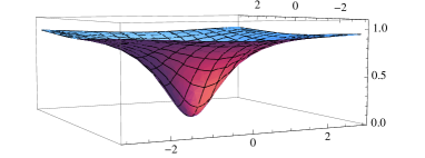
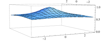
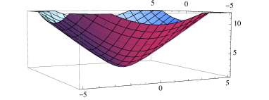
Figure 4: Upper left: the shape $\Phi(x)$ of the D4-brane for a single dyonic instanton. The instanton size is taken to be $\rho=1$, with $C=1$. Upper right: the shape $\Phi(p)$ for which the instanton size is given through the dispersion relation $\rho=m-\epsilon(p)$. Low: The electron dispersion given by $\epsilon=(m/2)/(\Phi(p)-1/2)$.

Now, let us use our dictionary (3.30) to relate the D4-brane shape (3.40) to the electron dispersion (3.28). Substituting the dictionary (3.30) to the first component (which represents a D4-brane among the pair) of (3.40), and choosing $C=2$ for simplicity (a scaling can recover the $C$ dependence anytime), we find

$$\Phi=\frac{(p_{\mu})^{2}}{(p_{\mu})^{2}+(m-\epsilon(p))^{2}}\,.$$ (3.41)

Using (3.28), we can eliminate the explicit $p_{\mu}$ dependence in this equation to finally obtain

$$\epsilon=\frac{m/2}{\Phi-1/2}\,.$$ (3.42)

This is the relation between the D4-brane shape $\Phi$ and the electron dispersion $\epsilon(p)$. See Fig. 4 for graphical images.

Remember that for the 2-dimensional system, the relation was found in (2.34) where the dispersion energy is given by the inverse of the scalar field. Here, we find the same equation; The energy is given by the inverse of the scalar field, and the inverse is measured from the asymptotic value of $\Phi$,

$$\Phi\rightarrow\frac{C}{4}=\frac{1}{2}\quad(p_{\mu}\rightarrow\infty)$$ (3.43)

Note that this is not inconsistent with the previous (3.39). When $p$ goes to $\infty$, $\epsilon(p)$ also scales. This means that through the identification (3.30), one needs to scale $\rho$ simultaneously.

In summary, we have found that the band $\epsilon(p)$ for the 4 dimensional class A system can be identified as the shape of a D-brane, under the exchange $x_{\mu}\leftrightarrow p_{\mu}$. The precise relation is given by (3.42) through the ADHM construction of dyonic instantons.

4 Chiral edge mode, noncommutative monopoles and tilted D-brane

So far, we have studied bulk properties and dispersions of electrons for 2-dimensional and 4-dimensional class A systems. On the other hand, the essential feature of topological materials is to have a surface massless state. In this section, we shall demonstrate that the dispersion of the chiral edge state for the 2-dimensional class A topological insulators can be understood again as the shape of a D-brane. The corresponding D-brane is a D-string which is tilted due to the spatial noncommutativity on the worldvolume of a D3-brane.

First we will give a brief review of the chiral edge state, then we turn to a review of the Nahm construction of a monopole in a noncommutative space. We will see a correspondence between the dispersion of the chiral edge state and the shape of the D-brane corresponding to the noncommutative monopoles.

4.1 Edge state and noncommutativity

First, we describe the chiral edge state appearing at a boundary of a 2-dimensional class A topological insulator, typically realized as the quantum Hall effect (see Ref. [20] for a comprehensive review). To introduce a boundary for the Hamiltonian (2.28) of the 2-dimensional system, let us consider an $x^{1}$-dependent mass term $m(x^{1})$, namely the domain-wall configuration. $x^{1}=0$ is the boundary of the 2-dimensional material, where the gap closes. To simplify the situation, we look at only the vicinity of the boundary, and approximate the region by a linear profile of the mass,

$$m(x^{1})=\theta x^{1}\,.$$ (4.1)

At $x^{1}=0$, the mass changes its sign, which indicates the boundary of the topological material such that the Chern number (2.38) is added once we cross the boundary line. The relevant Hamiltonian now reads

$${\cal H}=\sigma_{1}\theta x^{1}+\sigma_{2}p_{1}+\sigma_{3}p_{2}.$$ (4.2)

Due to the Heisenberg algebra $[\theta x^{1},p_{1}]=i\theta$, we define a creation/annihilation operator

$$\hat{a}\equiv\frac{1}{\sqrt{2\theta}}\left(\theta x^{1}+ip_{1}\right),\quad\hat{a}^{\dagger}\equiv\frac{1}{\sqrt{2\theta}}\left(\theta x^{1}-ip_{1}\right),$$ (4.3)

which satisfies $[\hat{a},\hat{a}^{\dagger}]=1$. (For simplicity, in this section we consider $\theta>0$.) The Hamiltonian is conveniently written as

$${\cal H}=\left(\begin{array}[]{cc}p_{2}&\sqrt{2\theta}\;\hat{a}^{\dagger}\\ \sqrt{2\theta}\;\hat{a}&-p_{2}\end{array}\right).$$ (4.6)

Let us remark that this Hamiltonian is equivalent to the 2-dimensional massive Dirac system in the presence of perpendicular magnetic field $B=\theta$, by replacing the momentum $p_{2}$ with the mass. In this sense, the dispersion relation shown in Fig. 5 is equivalent to the spectral flow with respect to the mass parameter of the corresponding system.

The energy eigenstates with energy $\epsilon$ can be easily obtained as

$$v_{0} = \left(\begin{array}[]{c}|0\rangle\\ 0\end{array}\right),\quad\epsilon=p_{2}$$ (4.9)

$$v_{n}^{\pm} = {\cal N}\left(\begin{array}[]{c}\sqrt{2\theta n}|n\rangle\\ (\epsilon-p_{2})|n-1\rangle\end{array}\right),\quad\epsilon=\pm\sqrt{2\theta n+(p_{2})^{2}}\quad(n\geq 1)$$ (4.12)

Note that the lowest mode is chiral, while higher modes are paired. The existence of this chiral edge mode $\epsilon=p_{2}$ is related to the topological number $\nu=1$, which is called bulk-edge correspondence. See, for example, a textbook on this topic [45].

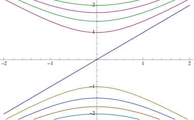
Figure 5: The dispersion relation of the states at the edge with $\theta=1$. The vertical axis is the energy $\epsilon$, and the horizontal axis is the momentum $p_{2}$. There exists a straight line $\epsilon=p_{2}$ which is the chiral edge state.

The energy is parameterized by a continuous momentum $p_{2}$ and the excited level $n$. This is contrast to the bulk state of the 2-dimensional system which is parameterized by the momenta $(p_{1},p_{2})$ and the mass $m$. Here, for the edge states, the noncommutativity between $m$ and $p_{1}$ is important and discretize the bulk state as if one has a magnetic field in the hypothetical $p_{1}$-$m$ plane.

If we look back our identification (2.31), we immediately notice that the corresponding D-brane configuration should be through a monopole in a non-commutative space,

$$[x^{1},x^{3}]=-i\theta.$$ (4.13)

The monopole in a noncommutative space was first predicted by D-brane configurations in string theory in Ref. [22] and explicitly constructed in Refs. [23, 24, 25].

4.2 The shape of tilted D1-brane and chiral edge state

The Nahm construction of monopoles in noncommutative space has been developed in Refs. [23, 24, 25] (see also Ref. [46]). The construction is almost the same as that in a commutative space. There are two differences: first, $\hat{x}^{1}$ and $\hat{x}^{3}$ need to be treated as operators, obviously, and second, the Nahm equation (2.2) is modified to

$$\frac{d}{d\xi}T_{i}=i\epsilon_{ijk}T_{j}T_{k}-\theta\delta_{i2}.$$ (4.14)

For a single $U(1)$ monopole, the simplest solution is

$$T_{2}=-\theta\xi,\quad T_{1}=T_{3}=0\,.$$ (4.15)

Therefore the zero-mode equation of the “Dirac operator” is

$$\left[\frac{d}{d\xi}+\theta\xi\sigma_{2}+\sigma_{i}x^{i}\right]v=0\,.$$ (4.16)

Note that here $\hat{x}^{1}$ and $\hat{x}^{3}$ are operators, and they do not commute. The last term can be identified with the electron Hamiltonian at the edge.

A variation of the noncommutative monopole solutions include so-called “fluxon” solution [24, 47]. It is a simple solution which is relevant to our study. The solution is given by the zero-mode

$$v=\left(\frac{\pi}{\theta}\right)^{1/4}\exp\left[-\frac{\theta}{2}\left(\xi+\frac{x_{2}}{\theta}\right)^{2}\right]\;\left(\begin{array}[]{c}|0\rangle\langle 0|\\ 0\end{array}\right)$$ (4.19)

One immediately notice a similarity to the chiral edge state (4.9). As the region of $\xi$ for this zero-mode is given by $-\infty<\xi<\infty$, we can evaluate the scalar field as

$$\Phi=\int_{-\infty}^{\infty}d\xi\;v^{\dagger}\xi v=-\frac{x_{2}}{\theta}|0\rangle\langle 0|$$ (4.20)

The scalar field configuration is linear in $x^{2}$. Indeed, the configuration was interpreted in string theory as a D1-brane piercing a D3-brane at an angle given by the noncommutativity. When $\theta=0$, the D1-brane becomes perpendicular to the D3-brane.

Since the Hamiltonian eigenvalues correspond to the operator $id/dt$ while the Nahm construction has $d/d\xi+\theta\xi$, from the formula $\Phi=\int d\xi\;v^{\dagger}\xi v$ we expect $\theta\Phi\sim\epsilon$. Indeed, comparing the D1-brane shape (4.20) and the dispersion of the chiral edge state (4.9), we find

$$\epsilon=-\theta\Phi\biggm{|}_{|0\rangle\langle 0|}$$ (4.21)

under the identification (2.31). So, the shape of the piercing D1-brane is the dispersion of the chiral edge state.

5 2D class AII and D-branes with orientifold

So far we studied class A systems which are fundamental examples responsible for the quantum Hall effect. Interesting topological insulators are offered with various other classes as shown in Table 1, and among them a popular topological insulator is class AII exhibiting the time-reversal symmetry. In this section we consider 2-dimensional class AII topological insulators and provide a D-brane interpretation of the band spectrum.

5.1 A brief review of helical edge state

The class AII topological insulators are protected by a time-reversal symmetry. A Hamiltonian of a free fermion which allows the time-reversal invariance can be obtained by a combination of two class A Hamiltonians (2.28) which amounts to introducing the spin degrees of freedom. In fact, it is a Dirac Hamiltonian in 3 dimensions with $p_{3}=0$,

$${\cal H}=(\sigma_{1}p_{1}+\sigma_{2}p_{2})\otimes\sigma_{2}+m\mathbf{1}_{2}\otimes\sigma_{3}\,.$$ (5.1)

Since in this Dirac representation the spin operator is given by $(\hbar/2)\sigma_{i}\otimes\mathbf{1}_{2}$, the time-reversal symmetry transformation is provided as

$$\Theta=(-i\sigma_{2})\otimes\mathbf{1}_{2}K$$ (5.2)

where $K$ is the complex conjugation operator and the matrix $(-i\sigma_{2})$ flips the sign of the spin operator. Under this operation, our Hamiltonian is transformed as follows,

$$\Theta:\quad{\cal H}(p) \rightarrow \Theta^{-1}{\cal H}(p)\Theta$$ (5.3)

$$=\left[(-i\sigma_{2})\otimes\mathbf{1}_{2}\right]^{-1}{\cal H}^{*}(p)\left[(-i\sigma_{2})\otimes\mathbf{1}_{2}\right]$$

$$={\cal H}(-p)\,.$$

This shows the time-reversal symmetry for the Bloch Hamiltonian for the present system, because $K$ changes the sign of the momenta $(p_{1},p_{2})\rightarrow(-p_{1},-p_{2})$ as is easily understood in the coordinate space representation. Obviously from the definition we have $\Theta^{2}=-1$, which corresponds, in Table 1, to the “$-$” sign in the class AII.

To obtain the helical edge state, we repeat the procedures given in the last section. First, consider the edge given by a mass profile $m(x^{1})=\theta x^{1}$. Then, together with the momentum $p_{1}$, these form the creation and annihilation operators,

$$m=\sqrt{\theta/2}(\hat{a}+\hat{a}^{\dagger}),\quad p_{1}=(-i)\sqrt{\theta/2}(\hat{a}-\hat{a}^{\dagger}).$$ (5.4)

Hamiltonian eigenvalue problem can be easily worked out to have two edge modes

$$v_{0}^{(1)}=\left(\begin{array}[]{c}|0\rangle\\ 0\\ 0\\ i|0\rangle\end{array}\right),\quad\epsilon=p_{2}\qquad\mbox{and}\qquad v_{0}^{(2)}=\left(\begin{array}[]{c}0\\ |0\rangle\\ i|0\rangle\\ 0\end{array}\right),\quad\epsilon=-p_{2}\qquad$$ (5.13)

These are helical edge modes, which are indicators of the class AII topological insulators. The dispersion relations of the other modes (4.12) degenerate, see Fig. 6.

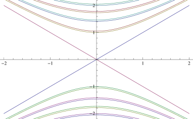
Figure 6: The dispersion relation of the states at the edge. The vertical axis is the energy $\epsilon$, and the horizontal axis is the momentum $p_{2}$. There are two straight lines $\epsilon=\pm p_{2}$ which are the helical edge states. Other gapped lines are doubly degenerate.

The class AII topological insulators have a topological number $\mathbb{Z}_{2}$. If one considers a deformation of the Hamiltonian (5.1) while keeping the time-reversal symmetry, the number of the pairs of the helical edge states should be kept odd. That is, the intersection of the two straight lines in Fig. 6 cannot be reconnected to form a mass gap.

5.2 Orientifold and helical edge state

We would like to realize the spectra of the helical edge modes, $\epsilon=\pm p_{2}$, in terms of the D-brane shape. As has been already constructed in the previous section, the dispersion of the chiral edge mode corresponds to the shape of a slanted D1-brane. So, one would think that we just need to duplicate the system such that we have two edge modes whose dispersion relations cross. However, the story is not that simple. the most important property of the class AII topological insulators is the $\mathbb{Z}_{2}$ charge. As emphasized at the end of the previous subsection, the helical edge modes should appear as an odd number of pairs. How this property can be seen in the D-brane shape is our goal of this section.

First, we need to re-interpret the Hamiltonian of the class AII, (5.1), in terms of the Nahm construction. Renaming the variables $(p_{1},p_{2},m)$ to the coordinates $(x^{1},x^{2},x^{3})$ as in (2.31), we can interpret the Hamiltonian as a Dirac operator of the Nahm construction, by further adding $\partial/\partial\xi$. At this stage, to make more use of the D-brane technique, we make use of the D-brane interpretation of the Dirac operator itself of the Nahm construction. The interpretation was given in Ref. [27]: the essential interpretation of the Dirac operator is a Hermitian tachyon field $T$ on a non-BPS D4-brane whose worldvolume completely contains the D1 and the D3-branes,

$$T=i\frac{\partial}{\partial\xi}+iu\left[(\sigma_{1}x^{1}+\sigma_{2}x^{2})\otimes(i\sigma_{2})+\mathbf{1}_{2}x^{3}\otimes\sigma_{3}\right]$$ (5.14)

where $u$ is a real positive parameter which will be taken to infinity for the tachyon to be on-shell. The four-dimensional space of the non-BPS D4-brane worldvolume is spanned by the coordinates $(x^{1},x^{2},x^{3},\xi)$.

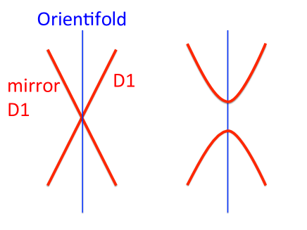
Figure 7: The effect of the orientifold in string theory. Left: a D1-brane intersects with the orientifold, yielding a mirror image of the D1-brane which appears to cross the original one at the orientifold. Right: A prohibited D-brane configuration. The D-brane intersects with the orientifold cannot be a single D1-brane. Intersection on the orientifold should accompany another D1-brane.

Now, we need to consider the time-reversal symmetry of the Hamiltonian. The D-brane interpretation of the time-reversal transformation should be

$$\Theta:\quad(x^{1},x^{2},x^{3},\xi)\rightarrow(-x^{1},-x^{2},x^{3},\xi),\quad T\rightarrow\left[(-i\sigma_{2})\otimes\mathbf{1}_{2}\right]^{-1}T^{*}\left[(-i\sigma_{2})\otimes\mathbf{1}_{2}\right]\,.$$ (5.15)

The equivalence to the time-reversal transformation for the Hamiltonian (5.3) is obvious.

Interestingly, this discrete transformation is equivalent to an orientifold transformation acting on the D4-brane. The orientifolding in string theory is given by

$$T\rightarrow J^{-1}T^{\rm T}J$$ (5.16)

accompanied by a target space parity. Since the tachyon field (and the Dirac Hamiltonian) is Hermitian, we have $T^{*}=T^{\rm T}$. The orientifolding $J$ is for defining a symplectic structure acting on the Chan-Paton factor of the non-BPS D4-branes, and our spin flip operation $(-i\sigma_{2})\otimes\mathbf{1}_{2}$ for the fermion Hamiltonian is identified with $J$. Therefore, the time-reversal invariance means the existence of an orientifold localized at $x^{1}=x^{2}=0$ in string theory.

Now, the consequence of the existence of the orientifold is important. It directly shows how D-brane configurations are consistent with band spectra of topological insulators (see Fig. 7).

• Existence of a mirror D-brane.

  Suppose we have a slanted D1-brane as in the previous section, $\epsilon=p_{2}$. Then the orientifold shows the existence of another D1-brane which is a mirror partner of the original D1-brane, $\epsilon=-p_{2}$. So the D1-branes cross each other and the intersection is on the orientifold.

  This shape of the D-branes is nothing but the pair of the helical edge states.

• D-brane intersect with the orientifold only as a pair.

  Upon the existence of the orientifold, it is known that D-branes crossing the orientifold fixed plane need to move as a pair [12, 49]. In other words, a single D1-brane intersecting with the orientifold is prohibited. Therefore the D1-brane intersecting with its mirror image cannot be reconnected.

  This means that the helical edge state is stable against any deformation preserving the time-reversal symmetry, and there is no way to produce a mass gap.

In summary, since the time-reversal invariance is identified with the existence of the orientifold in string theory under the dictionary (2.31), the dispersion relation of the helical edge state is interpreted as a D1-brane intersecting with its mirror image on the orientifold. No opening of a mass gap is consistent with the fact that D-branes needs to move as a pair on the orientifold.

6 Summary and discussions

In this paper, we showed that some dispersion relations and electron band spectrum of class A topological insulators are the shape of D-branes in string theory. The former is in a momentum space while the latter is in a coordinate space. The explicit dictionary between the momentum and the coordinate spaces is given as (2.31) and (3.30), and the relations between the electron bands and the shape of D-branes are given as (2.34) and (3.42). These examples are 2-dimensional and 4-dimensional class A topological insulators, corresponding to quantum Hall effects.

The correspondence was found through an analogy of the ADHM/Nahm construction of instantons and monopoles to the electron Hamiltonians of the topological insulators. The shape of D-branes is captured by a scalar field on the D-brane, and the scalar field detects the configuration of the topological solitons whose charge specify the topological properties of the electron system.

The correspondence between the electron band structure and the shape of D-branes was further generalized to the chiral and helical edge states. The corresponding D-brane configuration represents a monopole in non-commutative space which have been studied in string theory in details. We found that fluxon solutions (4.20) corresponds to the edge state, and indeed the shape of the D1-brane piercing the D3-brane corresponds to the dispersion of the chiral edge state. This interpretation is also possible for the system with time-reversal symmetry giving a helical edge state. On the D-brane side the time-reversal transformation is identified as an orientifolding, providing a mirror image of the slanted D1-brane, resulting in a crossing of the D1-branes at the orientifold. Opening a mass-gap is not allowed because the crossed D1-branes cannot be reconnected on the orientifold.

The intriguing part of the story is that D-brane picture is so intuitive that it enables us to study generalization of the system. As an example we studied the case with general integer value for the topological number $\nu$. It turns out that under the assumption of the BPS equation for the monopole and also under the assumption that the inter-layer interaction does not depend on momentum, all possible Hamiltonians having the general integer value $k$ of $\nu$ are characterized solely by the location of the $k$ monopoles in the space spanned by $(p_{1},p_{2},m)$.

In this paper we considered topological insulators only in 2 and 4 spatial dimensions. Obviously it would be interesting to further consider the case with 3 dimensions. The topological charge is ${\mathbb{Z}}_{2}$ for class AII system and the dispersion relation of the helical edge states will be given by some D-branes with an orientifold. In addition, in this manner, Hamiltonian systems with dimensions higher than 4 can be treated. Therefore, it would be interesting to discuss how to realize all the topological superconductors in the classification table along the direction studied in this paper.

D-branes have a lot of applications in string theory, and their shape can have various types. Spherical D-branes [50] and conic D-branes [51] appear in various context in string theory. General electron band structure can be compared with the shape of generic D-brane configurations. Intersecting D-branes reconnect as described by the worldvolume gauge theories [52], while electron bands reconnect generically in parameter space. More similarities and classifications due to our correspondence would be important for possible topological materials and also for string theory dynamics.

Acknowledgments

K. H. would like to thank M. Sato for valuable discussions. T. K. is grateful to Institut des Hautes Études Scientifiques for hospitality where a part of this work has been done. The work of K. H. was supported in part by JSPS KAKENHI Grant Numbers 15H03658, 15K13483. The work of T. K. was supported in part by JSPS KAKENHI Grant Number 13J04302.

References

- [1] A. Schnyder, S. Ryu, A. Furusaki, and A. Ludwig, “Classification of topological insulators and superconductors in three spatial dimensions,” Phys. Rev. B78 (2008) 195125, arXiv:0803.2786 [cond-mat.mes-hall].
- [2] A. Kitaev, “Periodic table for topological insulators and superconductors,” AIP Conf. Proc. 1134 (2009) 22–30, arXiv:0901.2686 [cond-mat.mes-hall].
- [3] J. Dai, R. G. Leigh, and J. Polchinski, “New Connections Between String Theories,” Mod. Phys. Lett. A4 (1989) 2073–2083.
- [4] J. Polchinski, “Combinatorics of boundaries in string theory,” Phys. Rev. D50 (1994) 6041–6045, arXiv:hep-th/9407031 [hep-th].
- [5] J. Polchinski, “Dirichlet Branes and Ramond-Ramond charges,” Phys. Rev. Lett. 75 (1995) 4724–4727, arXiv:hep-th/9510017 [hep-th].
- [6] E. Witten, “D-branes and K theory,” JHEP 12 (1998) 019, hep-th/9810188 [hep-th].
- [7] S. Ryu and T. Takayanagi, “Topological Insulators and Superconductors from D-branes,” Phys. Lett. B693 (2010) 175–179, arXiv:1001.0763 [hep-th].
- [8] S. Ryu and T. Takayanagi, “Topological Insulators and Superconductors from String Theory,” Phys. Rev. D82 (2010) 086014, arXiv:1007.4234 [hep-th].
- [9] A. Furusaki, N. Nagaosa, K. Nomura, S. Ryu, and T. Takayanagi, “Electromagnetic and thermal responses in topological matter: Topological terms, quantum anomalies and D-branes,” Comptes Rendus Physique 14 (2013) 871–883, arXiv:1211.0533 [cond-mat.mes-hall].
- [10] S. Ryu, A. P. Schnyder, A. Furusaki, and A. W. W. Ludwig, “Topological insulators and superconductors: Tenfold way and dimensional hierarchy,” New J. Phys. 12 (2010) 065010, arXiv:0912.2157 [cond-mat.mes-hall].
- [11] D. J. Thouless, M. Kohmoto, M. P. Nightingale, and M. den Nijs, “Quantized Hall Conductance in a Two-Dimensional Periodic Potential,” Phys. Rev. Lett. 49 (1982) 405–408.
- [12] E. Witten, “Small instantons in string theory,” Nucl. Phys. B460 (1996) 541–559, hep-th/9511030 [hep-th].
- [13] M. R. Douglas, “Branes within branes,” in Strings, Branes and Dualities, vol. 520 of NATO ASI Series, pp. 267–275. 1999. hep-th/9512077 [hep-th].
- [14] C. G. Callan and J. M. Maldacena, “Brane death and dynamics from the Born-Infeld action,” Nucl. Phys. B513 (1998) 198–212, hep-th/9708147 [hep-th].
- [15] W. Nahm, “A Simple Formalism for the BPS Monopole,” Phys. Lett. B90 (1980) 413.
- [16] M. F. Atiyah, N. J. Hitchin, V. G. Drinfeld, and Yu. I. Manin, “Construction of Instantons,” Phys. Lett. A65 (1978) 185–187.
- [17] E. Corrigan and P. Goddard, “Construction of Instanton and Monopole Solutions and Reciprocity,” Annals Phys. 154 (1984) 253.
- [18] P. Hořava, “Stability of Fermi surfaces and K-theory,” Phys. Rev. Lett. 95 (2005) 016405, hep-th/0503006 [hep-th].
- [19] S.-J. Rey, “String theory on thin semiconductors: Holographic realization of Fermi points and surfaces,” Prog. Theor. Phys. Suppl. 177 (2009) 128–142, arXiv:0911.5295 [hep-th].
- [20] G. E. Volovik, The Universe in a Helium Droplet. Oxford Univ. Press, 2009.
- [21] N. D. Lambert and D. Tong, “Dyonic instantons in five-dimensional gauge theories,” Phys. Lett. B462 (1999) 89–94, hep-th/9907014 [hep-th].
- [22] A. Hashimoto and K. Hashimoto, “Monopoles and dyons in noncommutative geometry,” JHEP 11 (1999) 005, hep-th/9909202 [hep-th].
- [23] D. J. Gross and N. A. Nekrasov, “Monopoles and strings in noncommutative gauge theory,” JHEP 07 (2000) 034, hep-th/0005204 [hep-th].
- [24] D. J. Gross and N. A. Nekrasov, “Dynamics of strings in noncommutative gauge theory,” JHEP 10 (2000) 021, hep-th/0007204 [hep-th].
- [25] D. J. Gross and N. A. Nekrasov, “Solitons in noncommutative gauge theory,” JHEP 03 (2001) 044, hep-th/0010090 [hep-th].
- [26] D.-E. Diaconescu, “D-branes, monopoles and Nahm equations,” Nucl. Phys. B503 (1997) 220–238, hep-th/9608163 [hep-th].
- [27] K. Hashimoto and S. Terashima, “Stringy derivation of Nahm construction of monopoles,” JHEP 09 (2005) 055, hep-th/0507078 [hep-th].
- [28] N. Drukker and B. Fiol, “All-genus calculation of Wilson loops using D-branes,” JHEP 02 (2005) 010, hep-th/0501109 [hep-th].
- [29] A. H. Castro Neto, F. Guinea, N. M. R. Peres, K. S. Novoselov, and A. K. Geim, “The electronic properties of graphene,” Rev. Mod. Phys. 81 (2009) 109–162, arXiv:0709.1163 [cond-mat.other].
- [30] Z. Liu, K. Suenaga, P. J. F. Harris, and S. Iijima, “Open and Closed Edges of Graphene Layers,” Phys. Rev. Lett. 102 (2009) 015501.
- [31] E. McCann and M. Koshino, “The electronic properties of bilayer graphene,” Rep. Prog. Phys. 76 (2013) 056503, arXiv:1205.6953 [cond-mat.mes-hall].
- [32] R. de Gail, M. O. Goerbig, F. Guinea, G. Montambaux, and A. H. Castro Neto, “Topologically protected zero modes in twisted bilayer graphene,” Phys. Rev. B84 (2011) 045436, arXiv:1103.3172 [cond-mat.mes-hall].
- [33] S.-C. Zhang and J. Hu, “A Four Dimensional Generalization of the Quantum Hall Effect,” Science 294 (2001) 823, arXiv:cond-mat/0110572.
- [34] X.-L. Qi, T. Hughes, and S.-C. Zhang, “Topological Field Theory of Time-Reversal Invariant Insulators,” Phys. Rev. B78 (2008) 195424, arXiv:0802.3537 [cond-mat.mes-hall].
- [35] S. Kim and K.-M. Lee, “Dyonic instanton as supertube between D-4 branes,” JHEP 09 (2003) 035, hep-th/0307048 [hep-th].
- [36] D. Mateos and P. K. Townsend, “Supertubes,” Phys. Rev. Lett. 87 (2001) 011602, hep-th/0103030 [hep-th].
- [37] R. Emparan, D. Mateos, and P. K. Townsend, “Supergravity supertubes,” JHEP 07 (2001) 011, hep-th/0106012 [hep-th].
- [38] D. Mateos, S. Ng, and P. K. Townsend, “Tachyons, supertubes and brane/anti-brane systems,” JHEP 03 (2002) 016, hep-th/0112054 [hep-th].
- [39] H.-Y. Chen, M. Eto, and K. Hashimoto, “The Shape of Instantons: Cross-Section of Supertubes and Dyonic Instantons,” JHEP 01 (2007) 017, hep-th/0609142 [hep-th].
- [40] K. Hashimoto and S. Terashima, “ADHM is tachyon condensation,” JHEP 02 (2006) 018, hep-th/0511297 [hep-th].
- [41] E. T. Akhmedov, “D-brane annihilation, renorm group flow and nonlinear sigma model for the ADHM construction,” Nucl. Phys. B592 (2001) 234–244, hep-th/0005105 [hep-th].
- [42] E. T. Akhmedov, A. A. Gerasimov, and S. L. Shatashvili, “On Unification of RR couplings,” JHEP 07 (2001) 040, hep-th/0105228 [hep-th].
- [43] M. Oshikawa, “Quantized Hall conductivity of Bloch electrons: Topology and the Dirac fermion,” Phys. Rev. B50 (1994) 17357–17363, cond-mat/9409079 [cond-mat].
- [44] N. Dorey, T. J. Hollowood, V. V. Khoze, and M. P. Mattis, “The Calculus of many instantons,” Phys. Rept. 371 (2002) 231–459, hep-th/0206063 [hep-th].
- [45] X.-G. Wen, Quantum Field Theory of Many-Body Systems: From the Origin of Sound to an Origin of Light and Electrons. Oxford Univ. Press, 2004.
- [46] M. Hamanaka, “ADHM/Nahm construction of localized solitons in noncommutative gauge theories,” Phys. Rev. D65 (2002) 085022, hep-th/0109070 [hep-th].
- [47] A. P. Polychronakos, “Flux tube solutions in noncommutative gauge theories,” Phys. Lett. B495 (2000) 407–412, hep-th/0007043 [hep-th].
- [48] B. A. Bernevig, T. L. Hughes, and S.-C. Zhang, “Quantum Spin Hall Effect and Topological Phase Transition in HgTe Quantum Wells,” Science 314 (2006) 1757, cond-mat/0611399 [cond-mat.mes-hall].
- [49] E. G. Gimon and J. Polchinski, “Consistency conditions for orientifolds and d manifolds,” Phys. Rev. D54 (1996) 1667–1676, arXiv:hep-th/9601038 [hep-th].
- [50] R. C. Myers, “Dielectric branes,” JHEP 12 (1999) 022, hep-th/9910053 [hep-th].
- [51] K. Hashimoto, S. Kinoshita, and K. Murata, “Conic D-branes,” PTEP 2015 (2015) 083B04, arXiv:1505.04506 [hep-th].
- [52] K. Hashimoto and S. Nagaoka, “Recombination of intersecting D-branes by local tachyon condensation,” JHEP 06 (2003) 034, hep-th/0303204 [hep-th].