Overlap distributions for quantum quenches in the anisotropic Heisenberg chain

Abstract

The dynamics after a quantum quench is determined by the weights of the initial state in the eigenspectrum of the final Hamiltonian, i.e., by the distribution of overlaps in the energy spectrum. We present an analysis of such overlap distributions for quenches of the anisotropy parameter in the one-dimensional anisotropic spin-1/2 Heisenberg model (XXZ chain). We provide an overview of the form of the overlap distribution for quenches from various initial anisotropies to various final ones, using numerical exact diagonalization. We show that if the system is prepared in the antiferromagnetic Néel state (infinite anisotropy) and released into a non-interacting setup (zero anisotropy, XX point) only a small fraction of the final eigenstates gives contributions to the post-quench dynamics, and that these eigenstates have identical overlap magnitudes. We derive expressions for the overlaps, and present the selection rules that determine the final eigenstates having nonzero overlap. We use these results to derive concise expressions for time-dependent quantities (Loschmidt echo, longitudinal and transverse correlators) after the quench. We use perturbative analyses to understand the overlap distribution for quenches from infinite to small nonzero anisotropies, and for quenches from large to zero anisotropy.

I Introduction and motivation

The past decade has witnessed a tremendous resurgence of interest in the physics of quantum many-body systems out of equilibrium 2011_Polkovnikov_RevModPhys_83_863 ; 2015_Eisert_NatPhys_11_124 ; 2010_Dziarmaga_AdvPhys_59_1063 . This growth has been partly motivated by remarkable developments in experiments, especially in experiments on cold atoms, which made the explicit observation of time evolution of many-body quantum systems possible 2002_Greiner_Nature_419_51 ; 2006_Kinoshita_Nature_440_900 ; 2012_Schneider_NaturePhys_8_213 ; 2012_Trotzky_Nature_8_325 ; 2007_Hofferberth_Nature_449_324 ; 2012_Cheneau_Nature_481_484 ; 2012_Gring_Science_337_1318 ; 2013_Ronzheimer_PRL_110_205301 ; 2007_Lee_PRL_99_020402 ; 2009_Palzer_PRL_103_150601 ; 2007_Trotzky_Science_319_295 . In addition to the experimental motivation, fundamental conceptual issues, such as thermalization in isolated systems and the nature of adiabaticity, have also played a strong role in driving the development of this field. A central paradigm in the study of non-equilibrium physics is the quantum quench. A quantum quench involves a protocol starting from the ground state (or a thermal state or another eigenstate) of an ‘initial’ Hamiltonian $H_{i}$, and then rapidly changing the Hamiltonian so that nontrivial time evolution occurs under a different (‘final’) Hamiltonian $H_{f}$. Many aspects of the dynamics induced by quantum quenches have been considered in recent years; the literature is rapidly growing and already too vast to review here.

A quantum quench can lead to nontrivial dynamics as the initial state generally has overlap with many eigenstates of the final Hamiltonian. If $|n\rangle$ and $E_{n}$ are the eigenstates and eigenvalues of the final Hamiltonian, i.e., $H_{f}|n\rangle=E_{n}|n\rangle$, an initial state $|\Psi_{0}\rangle$ will lead to the following time dependence of the system wavefunction:

$$|\Psi(t)\rangle=\mathrm{e}^{-\mathrm{i}H_{f}t}|\Psi_{0}\rangle=\mathrm{e}^{-\mathrm{i}H_{f}t}\sum_{n}c_{n}|n\rangle=\sum_{n}\mathrm{e}^{-\mathrm{i}E_{n}t}c_{n}|n\rangle\qquad\textnormal{with}\quad c_{n}=\langle n|\Psi_{0}\rangle\,.$$ (1)

If a large number of final eigenstates have non-negligible overlap $|c_{n}|$, this sum can lead to highly nontrivial time dependence. Clearly, both the overlaps $|c_{n}|=|\langle\Psi_{0}|n\rangle|$ and the corresponding eigenenergies $E_{n}$ are important in determining the subsequent dynamics. The object of study of the present paper is the distribution of overlaps, i.e., the overlap magnitudes $|c_{n}|$ as a function of energy $E_{n}$. We will refer to this as the “overlap distribution”. Note that, if the squares $|c_{n}|^{2}$ were considered, this could be regarded as a discrete probability distribution, as $\sum_{n}|c_{n}|^{2}=1$ and the squares $|c_{n}|^{2}$ represent probabilities. Since $|c_{n}|$ and $|c_{n}|^{2}$ provide equivalent information, we will focus on $|c_{n}|$. Also note that the distribution of phases of $c_{n}$ may provide useful information but are not individually well-defined, since the phases of individual eigenstates $|n\rangle$ can be chosen arbitrarily.

This work presents an investigation of the features of the overlap distribution for various quenches in a particular system. In this introductory section, we provide motivation for the study of the overlap distribution, by reviewing its connections to topics that have attracted widespread attention in recent years.

The overlap distribution is closely related to the statistics of the work performed in a quench, which is characterized by the so-called work distribution 1997_Jarzynski_PRL_78_2690 ; 2007_Talkner_PRE_75_050102 ; 2008_Silva_PRL_101_120603 ; 2011_Campisi_RMP_83_771 :

$$p(w)=2\pi\sum_{n}|c_{n}|^{2}\delta(w-(E_{n}-E_{i}))\,,$$ (2)

where $E_{i}$ is the initial energy. The work distribution is thus simply a continuous version of the distribution of squared overlaps, with the zero of the energy shifted by $E_{i}$. The work statistics in non-equilibrium processes in various quantum many-body systems is a topic of much recent interest 2008_Silva_PRL_101_120603 ; 2014_Shchadilova_PRL_112_070601 ; 2012_Dora_PRB_86_161109 ; 2009_Paraan_PRE_80_061130 ; 2010_Mossel_NewJPhys_12_055028 ; 2011_Gambassi_1106.2671 ; 2012_Heyl_PRL_108_190601 ; 2012_Gambassi_PRL_109_250602 ; 2012_Heyl_PRB_85_155413 ; 2012_Smacchia_PRL_109_037202 ; 2013_Dorner_PRL_110_230601 ; 2013_Mazzola_PRL_110_230602 ; 2013_Sotiriadis_PRE_87_052129 ; 2013_Smacchia_PRE_88_042109 ; 2014_Sindona_NJP_16_045013 ; 2014_Marino_PRB_89_024303 ; 2014_Palmai_PRE_90_052102 ; 2014_Fusco_PRX_4_031029 ; 2015_Dutta_PRE_92_012104 ; 2015_Palmai_1506.08200 . Another quantity of wide current interest, closely related to the overlap distribution and work distribution, is the return probability,

$$\mathcal{L}(t)=|\langle\Psi_{0}|\mathrm{e}^{-\mathrm{i}H_{f}t}|\Psi_{0}\rangle|^{2}=|\langle\Psi_{0}|\mathrm{e}^{\mathrm{i}H_{i}t}\mathrm{e}^{-\mathrm{i}H_{f}t}|\Psi_{0}\rangle|^{2}\,.$$ (3)

This is a special case of the Loschmidt echo where the reverse time evolution occurs under the Hamiltonian $H_{i}$, for which the initial state $|\Psi_{0}\rangle$ is an eigenstate. Following common practice, we will refer to this quantity simply as the Loschmidt echo. The behavior of the Loschmidt echo after a quantum quench has been studied in a large body of recent literature, see, e.g., 2008_Silva_PRL_101_120603 ; 2014_Andraschko_PRB_89_125120 ; 2012_Heyl_PRB_85_155413 ; 2014_Palmai_PRE_90_052102 ; 2011_Stephan_JStatMech_P08019 ; 2010_Mossel_NewJPhys_12_055028 ; 2013_Pozsgay_JStatMech_P10028 ; 2006_Quan_PRL_96_140604 ; 2014_Torres-Herrera_NJP_16_063010 ; 2015_Torres-Herrera_1506.08904 ; 2015_Torres-Herrera_PRB_92_014208 ; 2014_Torres-Herrera_PRA_90_033623 ; 2014_Torres-Herrera_PRE_89_062110 ; 2014_Torres-Herrera_PRA_89_043620 ; 2013_Torres-Herrera_PRE_88_042121 ; 2015_Viti_1507.08132 ; 2014_DeLuca_90_081403 ; 2013_Heyl_PRL_110_135704 ; 2014_Kennes_PRB_90_115101 ; 2014_Canovi_PRL_113_265702 ; 2015_Schmitt_PRB_92_075114 ; 2015_Rajak_1507.00963 ; 2012_Mukherjee_PRB_86_020301 ; 2012_Montes_PRE_86_021101 ; 2011_Jacobson_PRA_84_022115 ; 2011_CamposVenuti_PRL_107_010403 ; 2012_Happola_PRA_85_032114 ; 2010_CamposVenuti_PRA_81_022113 ; 2014_Campbell_PRA_90_013617 ; 2014_Vasseur_PRX_4_041007 ; 2013_Heyl_1310.6226 ; 2014_Sachdeva_PRB_90_045421 ; 2013_Karrasch_87_195104 ; 2013_Stephan_JSTAT_P09002 ; 2012_Lelas_PRA_86_033620 ; 2014_Kriel_PRB_90_125106 ; 2014_Heyl_PRL_113_205701 ; 2014_Hickey_PRB_89_054301 ; 2013_Dora_PRL_111_046402 ; 2014_Dora_1410.5954 ; 2013_Fagotti_1308.0277 ; 2014_Vajna_PRB_89_161105 ; 2014_Vajna_PRB_91_155127 . In particular, the Loschmidt echo is central to the study of so-called dynamical phase transitions 2013_Heyl_PRL_110_135704 ; 2014_Canovi_PRL_113_265702 ; 2013_Karrasch_87_195104 ; 2014_Hickey_PRB_89_054301 ; 2014_Heyl_PRL_113_205701 ; 2014_Andraschko_PRB_89_125120 ; 2015_Schmitt_PRB_92_075114 ; 2014_Kriel_PRB_90_125106 ; 2014_Vajna_PRB_89_161105 ; 2014_Vajna_PRB_91_155127 . By expanding $|\Psi_{0}\rangle$ in terms of the eigenstates $|n\rangle$ of the final Hamiltonian $H_{f}$, we find

$$\mathcal{L}(t)=\left|\sum_{n}\textnormal{e}^{-\mathrm{i}E_{n}t}|c_{n}|^{2}\right|^{2}=\left|\int{}\frac{d\omega{}}{2\pi}p(\omega)\mathrm{e}^{-\mathrm{i}{\omega}t}\right|^{2}\,.$$ (4)

Knowledge of the overlap distribution, i.e., the $|c_{n}|$’s and corresponding $E_{n}$’s, thus leads directly to the Loschmidt echo. For example, the energy width of the distribution determines the coefficient of the initial quadratic decay of $\mathcal{L}(t)$, as it can be seen by expanding $\mathrm{e}^{-\mathrm{i}H_{f}t}$ in Eq. (3) to second order in $t$ 2015_Viti_1507.08132 ; 2014_Torres-Herrera_PRA_89_043620 .

After a quench, a generic observable $\mathcal{O}$ has the following time evolution:

$$\langle\mathcal{O}(t)\rangle=\langle\Psi(t)|\mathcal{O}|\Psi(t)\rangle=\langle\Psi_{0}|\mathrm{e}^{\mathrm{i}H_{f}t}\mathcal{O}\mathrm{e}^{-\mathrm{i}H_{f}t}|\Psi_{0}\rangle=\sum_{m,n}c_{m}^{\ast}c_{n}\mathrm{e}^{-\mathrm{i}(E_{n}-E_{m})t}\langle m|\mathcal{O}|n\rangle\xrightarrow{t\to\infty}\sum_{n}|c_{n}|^{2}\langle n|\mathcal{O}|n\rangle\,.$$ (5)

The long-time behavior of such expectation values, $\lim_{t\to\infty}\langle\mathcal{O}(t)\rangle$, is of fundamental interest since this is closely related to the question of whether an isolated quantum system thermalizes in some sense. As outlined above, this long-time limit is determined solely by the overlap magnitudes and the diagonal matrix elements. This is often called the “diagonal ensemble” value of the long-time limit 2008_Rigol_Nature_452_854 . The eigenstate thermalization hypothesis (ETH), which is expected to hold for non-integrable systems, postulates that the diagonal matrix elements $\langle n|\mathcal{O}|n\rangle$ are smooth functions of eigenenergy, for large enough systems 1994_Srednicki_PRE_50_888 ; 1991_Deutsch_PRA_43_2046 ; 2008_Rigol_Nature_452_854 ; 2012_Neuenhahn_PRE_85_060101 ; 2014_Beugeling_PRE_89_042112 . The question of thermalization can then reduce to the question of how narrow in energy the overlap distribution is. Recent work (such as the “quench action” approach 2013_Caux_PRL_110_257203 ; 2014_DeNardis_PRA_89_033601 ; 2014_Wouters_PRL_113_117202 ; 2014_Pozsgay_PRL_113_117203 ; 2014_Brockmann_JStatMech_P12009 ; 2015_DeLuca_PRA_91_021603 ; 2015_Ilievski_1507.02993 and an approach based on linked-cluster expansions 2014_Rigol_PRL_112_170601 ; 2014_Rigol_PRE_90_031301 ) has formulated calculations of long-time expectation values directly in the thermodynamic limit, thus avoiding the explicit calculation of overlaps in finite-size systems. The diagonal ensemble formulation of Eq. (5) for finite sizes, involving the overlap distribution $|c_{n}|$, will play an essential role in the discussion of such calculations for long-time stationary state values of observables, in particular for comparing the ordering of the limiting procedures (limits of large sizes and large times). We also note that the overlaps $c_{n}$ appear not only in the long-time limit, but also in the arbitrary-time expression for $\langle\mathcal{O}(t)\rangle$ (cf. Eq. (5)), although in this case the phases of $c_{n}$ are also important.

From the discussion above, it is clear that the overlap distribution plays a central role in many aspects of quench dynamics. Numerical data on overlap distributions have appeared in many different non-equilibrium studies for specific quenches, e.g., in Refs. 2015_Torres-Herrera_1506.08904 ; 2015_Torres-Herrera_PRB_92_014208 ; 2014_Torres-Herrera_PRA_90_033623 ; 2014_Torres-Herrera_PRE_89_062110 ; 2013_Torres-Herrera_PRE_88_042121 ; 2014_Torres-Herrera_NJP_16_063010 ; 2014_Torres-Herrera_PRA_89_043620 where the overlap distributions are called “local density of states”, in Refs. 2008_Rigol_Nature_452_854 ; 2011_Cassidy_PRL_106_140405 ; 2011_Rigol_PRA_84_033640 ; 2011_Santos_PRL_107_040601 ; 2014_Sorg_PRA_90_033606 ; 2009_Rigol_PRA_80_053607 ; 2010_Biroli_PRL_105_250401 in the context of thermalization, in Ref. 2014_Shchadilova_PRL_112_070601 in connection with intermediate-time behaviors of the Loschmidt echo, and in Ref. 2014_Hild_PRL_113_147205 for a spin spiral initial state. There have been, however, relatively few systematic studies of the overlap distribution so far. The present work is a step towards addressing this gap in the literature.

We provide a detailed study of the overlap distribution for a well-known model system, namely the one-dimensional anisotropic spin-1/2 Heisenberg model (XXZ chain) at zero magnetization. We consider quenches of the anisotropy parameter $\Delta$, see Eq. (6), and provide an overview of the overlap distributions obtained in quenches from various initial $\Delta_{i}$ values to various final $\Delta_{f}$ values, using full numerical diagonalization. For the special case of $\Delta_{i}=\infty$ and $\Delta_{f}=0$, i.e., quenching from the Néel state to the so-called XX point, we present a full analytical study of the overlap distribution. The XX point is mappable to a chain of free fermions, which allows this detailed analysis. We find that all nonzero overlaps are exactly equal and derive expressions for them, using the Slater determinant structure of the XX eigenfunctions, as well as using the Bethe ansatz. We derive the selection rules determining the eigenstates that have nonzero overlaps for this quench, both in the language of fermionic momenta and using the language of Bethe roots. We show how these results on the overlap distribution can be used to derive explicit expressions for the Loschmidt echo $\mathcal{L}(t)$ and for equal-time correlators after the quench. For quenches ending at small but nonzero anisotropy, $\Delta_{f}\ll 1$, a splitting structure appears in the overlap distribution; we analyze the main features of this structure using perturbation theory. Similarly, for quenches to the XX point starting from large but finite initial value $\Delta_{i}\gg 1$, a perturbative expansion in $1/\Delta_{i}$ explains the structure of the overlap distribution.

After introducing the model and some notation in Sec. II, we provide our numerical overview of overlap distributions in quenches from various $\Delta_{i}$ to various $\Delta_{f}$ in Sec. III. Section IV is devoted to a detailed analysis of the $\Delta_{i}=\infty\to\Delta_{f}=0$ case. We also use the results for the overlap distribution to derive analytical expressions for time-dependent quantities, in particular, for the Loschmidt echo and for longitudinal and transverse two-point correlators. Section V outlines a perturbative treatment of the $\Delta_{i}=\infty\to\Delta_{f}\ll 1$ case (perturbation in $\Delta_{f}$), while Sec. VI describes a perturbative treatment of the $\Delta_{i}\gg 1\to\Delta_{f}=0$ case (perturbation in $1/\Delta_{i}$).

II The model

This work focuses on the one-dimensional anisotropic spin-1/2 Heisenberg model (XXZ chain) with nearest-neighbor interactions. The Hamiltonian is given by

$$H=\sum_{j=1}^{L}\left(S_{j}^{x}S_{j+1}^{x}+S_{j}^{y}S_{j+1}^{y}+\Delta S_{j}^{z}S_{j+1}^{z}\right)=\frac{1}{2}\sum_{j=1}^{L}\left(S_{j}^{+}S_{j+1}^{-}+S_{j}^{-}S_{j+1}^{+}\right)+\Delta\sum_{j=1}^{L}S_{j}^{z}S_{j+1}^{z}=H_{\text{xx}}+\Delta H_{z}\,,$$ (6)

where $S_{j}^{\alpha}=\sigma_{j}^{\alpha}/2$, $\alpha=x,y,z$, with $\sigma_{j}^{\alpha}$ being the usual Pauli matrices, and $S_{j}^{\pm}=S_{j}^{x}\pm\mathrm{i}S_{j}^{y}$. We will refer to the $\Delta=0$ part of the Hamiltonian as the XX Hamiltonian: $H_{\text{xx}}=\frac{1}{2}\sum_{j=1}^{L}\left(S_{j}^{+}S_{j+1}^{-}+S_{j}^{-}S_{j+1}^{+}\right)$. Throughout this manuscript we choose the number $L$ of lattice sites to be even. We also distinguish between two different types of boundary conditions. For an open chain we set $S_{L+1}^{\alpha}=0$, for a periodic chain $S_{L+1}^{\alpha}=S_{1}^{\alpha}$, $\alpha=x,y,z$.

The XXZ chain is a natural generalization of the isotropic Heisenberg chain 1928_Heisenberg_ZPhys_49_619 . It is one of the most widely studied models in quantum magnetism in particular, and condensed matter physics in general. It is absolutely central to the study of integrability, having a relatively simple integrable structure, yet possessing rich physics and displaying a phase transition. In the current era of non-equilibrium physics, it has been widely used as a model system to explore and exemplify non-equilibrium phenomena, including studies of the Loschmidt echo (e.g. 2010_Mossel_NewJPhys_12_055028 ; 2014_Andraschko_PRB_89_125120 ; 2013_Dora_PRL_111_046402 ; 2014_Dora_1410.5954 ; 2013_Fagotti_1308.0277 ; 2014_Heyl_PRL_113_205701 ; 2014_Torres-Herrera_PRA_89_043620 ), studies of quenches of the anisotropy parameter $\Delta$ (e.g. 2010_Barmettler_NewJPhys_12_055017 ; 2015_Collura_1507.03492 ), and of quenches starting from a Néel state (e.g. 2014_Wouters_PRL_113_117202 ; 2010_Barmettler_NewJPhys_12_055017 ; 2014_Fagotti_PRB_89_125101 ; 2014_Pozsgay_PRL_113_117203 ; 2014_Brockmann_JStatMech_P12009 ; 2014_Heyl_PRL_113_205701 ; 2014_Torres-Herrera_PRA_89_043620 ). Dynamics starting from various non-uniform states (such as domain wall initial states), leading to propagation or transmission along the XXZ chain, is also a rapidly growing topic of investigation (see, e.g., 2014_Liu_PRL_112_257204 ; 2014_Alba_PRB_90_075144 ; 2005_Gobert_PRE_71_036102 ; 2010_Mossel_NewJPhys_12_055028 ; 2013_Misguich_PRB_88_245114 ; 2013_Ganahl_1302.2667 ; 2012_Woellert_PRB_85184433 ; 2009_Langer_PRB_79_214409 ; 2010_Haque_PRA_82_012108 ; 2011_Jesenko_PRB_84_174438 ; 2014_Karrasch_PRB_89_075139 ; 2014_Sharma_PRA_89_043608 ; 2014_DeLuca_PRB_90_161101 ; 2013_Karrasch_PRB_88_195129 ; 2012_Karrasch_PRL_108_227206 ; 2011_Langer_PRB_84_205115 ; 2015_Vlijm_1507.08624 ). The XXZ chain is also being increasingly used to study real-time thermal transport and real-time dynamics at finite temperatures 2012_Karrasch_PRL_108_227206 ; 2014_Karrasch_PRB_89_075139 ; 2013_Karrasch_PRB_88_195129 ; 2014_Bonnes_PRL_113_187203 ; 2011_Langer_PRB_84_205115 ; 2014_DeLuca_PRB_90_161101 . It is a primary testbed for developments and applications of Bethe ansatz techniques for addressing non-equilibrium issues (e.g. 2010_Mossel_NewJPhys_12_055028 ; 2014_Goldstein_90_043625 ; 2014_Liu_PRL_112_257204 ; 2015_Alba_91_155123 ; 2014_Pozsgay_JStatMech_P06011 ; 2014_Brockmann_JPA_47_145003 ; 2014_Brockmann_JPA_47_345003 ; 2013_Caux_PRL_110_257203 ; 2014_DeNardis_PRA_89_033601 ; 2014_Wouters_PRL_113_117202 ; 2015_Vlijm_1507.08624 ; 2014_Pozsgay_PRL_113_117203 ; 2014_Brockmann_JStatMech_P12009 ; 2013_Alba_2013_JStatMech_P10018 ). We therefore find the XXZ chain to be an appropriate model for a systematic study of the work distribution in quantum quenches.

In this work, we restrict to positive anisotropies $\Delta>0$. The isotropic critical point $\Delta=1$ separates two regimes with different behaviors; in terms of low-energy physics, the $\Delta<1$ regime is gapless, while the $\Delta>1$ regime is gapped. The Hamiltonian (6) commutes with the $z$-component $S^{z}=\sum_{j=1}^{L}S_{j}^{z}$ of the total spin operator. For even $L$ the zero magnetization sector contains the ground state for all $\Delta>1$. Our initial states are ground states of the XXZ chain and, hence, lie in the zero magnetization sector. Thus, we can restrict to the subspace spanned by energy eigenstates $|n\rangle$ with $S^{z}|n\rangle=0$. At $\Delta=0$ the chain can be mapped onto a gas of free fermions via the Jordan-Wigner mapping, and subsequently solved using free-fermion techniques. For generic values of the anisotropy parameter $\Delta$ the XXZ model is integrable and can be solved by means of Bethe Ansatz techniques 1931_Bethe_ZPhys_71_205 ; BaxterBOOK ; GaudinBOOK ; KorepinBOOK ; 1988_Sklyanin_JPhysA_21_2375 . In the fermionic language the anisotropy $\Delta$ acts as the strength of nearest-neighbor interactions.

A particular focus of this work will be on quenches starting from the purely antiferromagnetic regime ($\Delta_{i}\to\infty$). In the limit $\Delta_{i}\to\infty$ the initial Hamiltonian effectively becomes the Ising Hamiltonian, $H_{i}\sim H_{\rm Ising}=\sum_{j=1}^{L}S_{j}^{z}S_{j+1}^{z}$. The ground state of $H_{\rm Ising}$ is exactly degenerate, with both symmetric and antisymmetric combinations of the Néel states having the same energy. For $\Delta_{i}$ large but finite this degeneracy is lifted. We denote the two Néel states as

$$|N_{1}\rangle=\left|\uparrow\downarrow\right\rangle^{\otimes L/2}\qquad\text{and}\qquad|N_{2}\rangle=\left|\downarrow\uparrow\right\rangle^{\otimes L/2}\,.$$ (7)

For $\Delta_{i}=\infty$, any linear combination of $|N_{1}\rangle$ and $|N_{2}\rangle$ is a valid ground state and, in principle, any such linear combination could be chosen as the initial state with which to calculate overlaps. Physically, we find it most reasonable to choose the symmetric combination for $L/2$ even and the antisymmetric combination for $L/2$ odd, which is adiabatically connected to the (unique) ground state for $\Delta_{i}$ large but finite,

$$|\Psi_{\sigma}\rangle=\frac{1}{\sqrt{2}}\left(|N_{1}\rangle+\sigma|N_{2}\rangle\right)\qquad\textnormal{with}\quad\sigma=(-1)^{L/2}\,.$$ (8)

For the periodic chain we set $\sigma=\mathrm{e}^{\mathrm{i}p_{0}}$ with $p_{0}=0,\pi$. Since $\hat{T}|\Psi_{\sigma}\rangle=\mathrm{e}^{\mathrm{i}p_{0}}|\Psi_{\sigma}\rangle$, where $\hat{T}$ is the translation operator by one lattice site, $p_{0}$ is nothing but the momentum of the initial state. For the open chain, $\sigma$ is related to the symmetry of $|\Psi_{\sigma}\rangle$ under reflection, $\mathscr{R}|\Psi_{\sigma}\rangle=\sigma|\Psi_{\sigma}\rangle$, where the reflection operator $\mathscr{R}$ maps lattice site $j$ to $L+1-j$ for all $j=1,\ldots,L$.

Recently, some progress has been made in calculating overlaps using the Bethe ansatz 2014_Pozsgay_JStatMech_P06011 ; 2014_Brockmann_JPA_47_145003 ; 2014_Brockmann_JPA_47_345003 ; 2014_Piroli_JPhysA_47_385003 . There are now exact formulas for the overlap between a Néel state and any eigenstate in terms of the Bethe roots describing the eigenstate 2014_Brockmann_JPA_47_145003 ; 2014_Brockmann_JPA_47_345003 ; 2014_Pozsgay_JStatMech_P06011 ; 2012_Kozlowski_JStatMech_P05021 ; 1998_Tsuchiya_JMathPhys_39_5946 . By taking the thermodynamic limit of the results of Ref. 2014_Brockmann_JPA_47_145003 , it was possible to investigate the long-time limit in quenches to the antiferromagnetic gapped phase $\Delta_{f}>1$ 2014_Wouters_PRL_113_117202 ; 2014_Pozsgay_PRL_113_117203 ; 2014_Brockmann_JStatMech_P12009 and also to the isotropic point $\Delta_{f}=1$ 2014_Brockmann_JStatMech_P12009 , using the quench action approach 2013_Caux_PRL_110_257203 . However, extracting all the overlaps for large but finite chains by means of the exact formulas of Refs. 2014_Brockmann_JPA_47_145003 ; 2014_Brockmann_JPA_47_345003 is technically quite challenging. For this reason, in this work we will use these forumlas only in the limit $\Delta_{f}\to 0$, where the structure of Bethe roots is well understood.

III Features of the overlap distribution: numerical overview

In this section we present an overview of the features of overlap distributions for quenches from various $\Delta_{i}$ to various $\Delta_{f}$, obtained using numerical exact diagonalization. We present overlaps with only those eigenstates of the post-quench Hamiltonian $H_{f}$ that lie in the zero magnetization sector. Since the initial states are always in this sector, eigenstates of $H_{f}$ in other magnetization sectors have zero overlap due to symmetry.

In cases where eigenstates of $H_{f}$ are (nearly or exactly) degenerate, numerical diagonalization might give overlaps with arbitrary linear combinations of the (nearly) degenerate eigenstates. In all cases where we discuss visible features of the overlap distribution, we have taken care to resolve such degeneracies. There are more degeneracies for periodic chains, so we show mainly open-chain data. We have checked in each case that the qualitative features are very similar for open and periodic chains.

III.1 Quench from $\Delta_{i}=\infty$ to $\Delta_{f}=0$

As explained in Sec. II, for quenches starting from $\Delta_{i}=\infty$ we choose as the initial state $\ket{\Psi_{0}}$ the combination $\ket{\Psi_{\sigma}}$ of Néel states as defined in Eq. (8). Overlap distributions for $\Delta_{i}=\infty$ to $\Delta_{f}=0$ quenches are shown in Fig. 1, for both open and periodic chains. The remarkable feature of these distributions is that the overlaps are either zero or have exactly equal nonzero value. There is no reason to expect that the ground state at $\Delta=\infty$ should have any particular preference between low-energy and high-energy eigenstates of the $\Delta=0$ Hamiltonian. Nevertheless, such a physical argument does not suffice to predict that the nonzero overlaps should all be exactly equal. This is a particular feature of the Néel-to-XX quench in the XXZ chain.

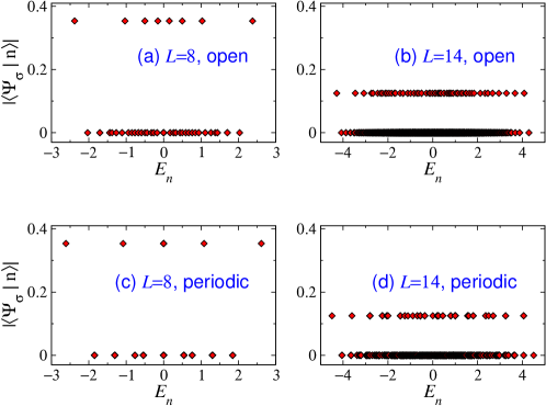
Figure 1: Overlap distributions for the quench $\Delta_{i}=\infty\to\Delta_{f}=0$. Data are shown for both open and periodic chains, for two different system sizes. There are $2^{L/2-1}$ nonzero overlaps, all exactly equal to $2^{-L/4+1/2}$ which is $2^{-3/2}\approx 0.354$ for $L=8$ and $2^{-3}=0.125$ for $L=14$. In the periodic cases some of the nonzero overlaps are not visually distinguishable because of degeneracies, e.g., in panel (c) there are four degenerate nonzero overlaps at $E_{n}=0$.

Among the $\binom{L}{L/2}$ final eigenstates in the zero magnetization sector, only $2^{L/2-1}$ have nonzero $c_{n}$’s. The number of nonzero overlaps fixes the nonzero values to be $|c_{n}|=2^{-L/4+1/2}$, by virtue of normalization and the fact that they are all equal. The counting can sometimes be tricky due to degeneracies. For example, there appears to be only five instead of eight nonzero overlaps in the $L=8$ periodic case in Fig. 1(c). This is because the symbol at the center represents four exactly degenerate eigenstates, which cannot be distinguished. There are also few eigenstates with the same eigenenergy but zero overlap. Of course, any linear combination of the degenerate eigenstates is also a valid eigenstate. So, there is some ambiguity in the overlaps plotted. By choosing the eigenstates to be the appropriate ‘Slater determinants’ in fermionic language (see Sec. IV), the overlaps turn out to be either zero or $|c_{n}|=2^{-L/4+1/2}$.

The overlap distribution for quenches from $\Delta_{i}=\infty$ to $\Delta_{f}=0$ will be analyzed in detail in Sec. IV, in particular we will derive the selection rules, which determine whether or not an eigenstate has nonzero overlap. We will also exploit this analysis to obtain closed expressions for time-dependent quantities.

III.2 Quenches from $\Delta_{i}=\infty$ to various nonzero $\Delta_{f}$

We now consider quenches starting from the $\ket{\Psi_{\sigma}}$ state ($\Delta_{i}=\infty$) to various nonzero values of $\Delta_{f}$.

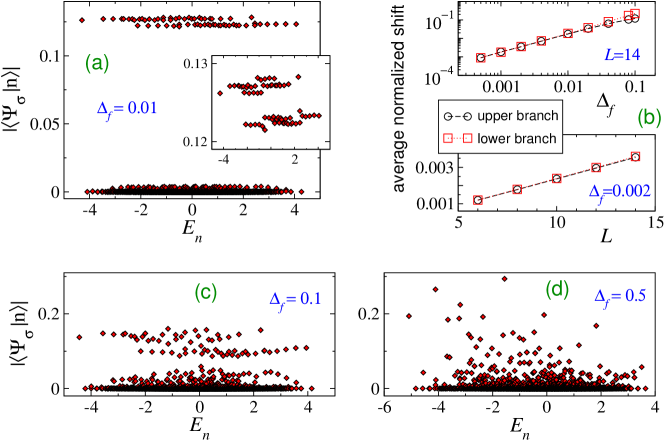
Figure 2: (a,c,d) Overlap distributions for $\Delta_{i}=\infty$ (initial state $\ket{\Psi_{0}}=\ket{\Psi_{\sigma}}$) in an open chain with $L=14$ sites. The splitting that can be observed for $\Delta_{f}\ll 1$ disappears as $\Delta_{f}$ grows. (b) Magnitude of the average normalized shifts for the two branches as function of $\Delta_{f}$ (double logarithmic scale) and as function of system size $L$ (linear scale). The normalized shift for small $\Delta_{f}$ is observed to be linear in $\Delta_{f}$ and $L$.

In Fig. 2(a,c,d), we show overlap distributions for quenches to $\Delta_{f}$ values in the gapless region, $\Delta_{f}<1$. When $\Delta_{f}$ is very small, the distribution is only slightly distorted from the $\Delta_{f}=0$ case, as expected from perturbative arguments. However, the pattern of distortion is rather remarkable. The $2^{L/2-1}$ nonzero overlaps now split into two well-defined branches; one branch is shifted upwards and one branch is shifted downwards, see Fig. 2(a). The upward- (resp. downward-) shifted branch is biased toward lower (resp. higher) energies. In particular, among the eigenstates satisfying the selection rule, the lowest few all have positive shift, the highest few always have negative shift, and the eigenstates with intermediate energies can have either positive or negative shift. In addition, many of the overlaps that were zero for the $\Delta_{f}=0$ case, now have nonzero (albeit tiny) $|c_{n}|$ values.

We will refer to the difference $|c_{n}|-2^{-L/4+1/2}$ of the absolute value of the Néel overlap with an eigenstate of the $\Delta_{f}\ll 1$ Hamiltonian and the Néel overlap at $\Delta_{f}=0$, i.e., $2^{-L/4+1/2}$, as the “shift” of the overlap. The splitting structure is well-defined as long as the shift is much smaller than $2^{-L/4+1/2}$; otherwise the lower branch is difficult to distinguish from the states with near-zero overlap. It is useful to normalize the shift with respect to the $\Delta_{f}=0$ value, i.e., for each eigenstate connected to one having nonzero overlap at $\Delta_{f}=0$, we define

$$\text{normalized shift}=\frac{\text{shift}}{2^{-L/4+1/2}}=\frac{|c_{n}|-2^{-L/4+1/2}}{2^{-L/4+1/2}}\,.$$ (9)

In Fig. 2(b), the magnitudes of the normalized shifts are averaged over the eigenstates in each branch. We see this to be linear with $\Delta_{f}$ at fixed $L$, and linear with $L$ at fixed $\Delta_{f}$, i.e., proportional to $L\Delta_{f}$. This indicates that the shift can be calculated perturbatively in $\Delta_{f}$ for any finite chain. However as the chain size gets larger the perturbative region of $\Delta_{f}$ shrinks. In Sec. V we will analyze the splitting and shift using first-order perturbation theory. The branches have internal structures, e.g., the overlap values roughly increase with energy within each branch.

For a fixed $L$, as $\Delta_{f}$ increases further, the splitting structures gets diffuse, and the separation between the $2^{L/2}$ larger values and the rest smaller values also gets obscured, see Fig. 2(c). Eventually, there is no visible remnant of the characteristic structure at $\Delta_{f}=0$, as seen for $\Delta_{f}=0.5$ in Fig. 2(d). For $\Delta_{f}=0.5$ the overlap distribution has no striking pattern, and no obvious remnant of the flat distribution at $\Delta_{f}=0$. A slight bias toward smaller energies is visible. This may be expected because, for any finite $\Delta_{f}>0$, the $\Delta_{i}=\infty$ ground state $\ket{\Psi_{\sigma}}$ should have more weight in the lower part of the spectrum than in the upper part.

This trend gets more prominent at larger $\Delta_{f}$. In Fig. 5 we show some examples for $\Delta_{f}>1$. The bias toward lower-energy states gets progressively stronger. This indicates that for quenches from $\Delta_{i}=\infty$ to $\Delta_{f}>1$, the dynamical evolution will be determined mostly by low-energy states. For $\Delta_{f}\gtrsim 3$ the ground state dominates the overlap distribution very strongly.

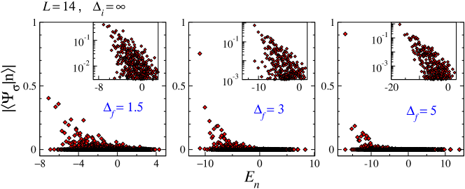
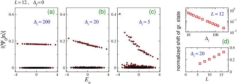
Figure 3: Overlap distributions for $\Delta_{i}=\infty$ (initial state $\ket{\Psi_{0}}=\ket{\Psi_{\sigma}}$) and $\Delta_{f}>1$ in an open chain with $L=14$ sites. The overlap distributions decay with increasing energy. The insets show the same data in a logarithmic scale.

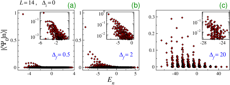
Figure 4: (a,b,c) Overlap distributions for $\Delta_{i}\gg 1$ and $\Delta_{f}=0$ in an open chain with $L=12$ sites. (d) The normalized shift of the lowest-energy eigenstate, as a function $\Delta_{i}$ for fixed chain length $L$ (double logarithmic scale), and as a function of chain length $L$ for fixed $\Delta_{i}$ (linear scale).

Figure 5: Overlap distributions for $\Delta_{i}=0$ and various $\Delta_{f}$ in an open chain with $L=14$ sites. In the last panel we see how for large values of $\Delta_{f}$ the energy spectrum is organized in ‘bands’.

III.3 Quenches from $\Delta_{i}\gg 1$ to $\Delta_{f}=0$

We now consider quenches to $\Delta_{f}=0$, starting from $\Delta_{i}\gg 1$ large but finite. The initial state $|\Psi_{0}\rangle$ is now no longer exactly the combination $\ket{\Psi_{\sigma}}$ of Néel states. From perturbative intuition, we expect that as $\Delta_{i}$ decreases toward smaller values the overlap distribution will deviate gradually from the characteristic shape of Fig. 1. This is seen to be true in Fig. 5, where we have plotted overlap distributions for an open chain with $L=12$, for three different $\Delta_{i}\gg 1$. The $2^{L/2-1}$ nonzero values exhibit a roughly linear dependence on $E_{n}$ as $\Delta_{i}$ is decreased from $\infty$. One expects the ground state at any finite $\Delta_{i}$ to be closer to the low-energy eigenstates of the $\Delta_{f}=0$ than to the higher-energy eigenstates. Hence, it is not surprising that the slope of the line is negative. The set of overlaps fall on a very nearly linear curve for large $\Delta_{i}$. For moderate $\Delta_{i}$, see Fig. 5(c), the overlaps follow a more curved line and show more scatter. In addition the near-zero overlap values start to be noticeable.

The shift of the ground state overlap from $2^{-L/4+1/2}$ can be seen numerically to scale as $\propto 1/\Delta_{i}$ for a given $L$ and large $\Delta_{i}$, see Fig. 5(d). The overlap of the highest-energy eigenstate obeying the selection rules scales in the same way. Also, the normalized shift for the ground state scales linearly with chain length $L$ for a given $\Delta_{i}$.

In Sec. VI, treating the XX part of the Hamiltonian as a perturbation to the Ising Hamiltonian, we will show that the shift of the overlaps is exactly a linear function of energy at first order in $1/\Delta_{i}$. In fact, the normalized shift for the eigenstates satisfying the selection rule will be shown to be $-E_{n}/\Delta_{i}$ at first order (exact for periodic chains, approximate up to order $1/L$ for open chains), consistent with the numerical data.

III.4 Quenches from $\Delta_{i}=0$ to various $\Delta_{f}$

We now consider quenches starting from $\Delta_{i}=0$. Thus, the initial state is the ground state of a free fermionic Hamiltonian. Examples for three $\Delta_{f}$ values are shown in Fig. 5 for an $L=14$ open chain. For any finite value of $\Delta_{f}$, we expect a bias toward low-energy states. This is seen in all three cases. The bias is naturally stronger for smaller $\Delta_{f}$. We see that up to $\Delta_{f}=2$ the ground state overlap dominates the overlap distribution. Other than the ground state, most of the weight for $\Delta_{f}\approx 1$ goes to a few final eigenstates at relatively low energies. We also see from the logarithmic plots in the insets of Fig. 5(a,b) that there is a characteristic decaying shape. The upper envelope of this scatter-plot decays roughly exponentially, although a sharp qualitative statement about the decay rate is difficult to make, due to finite-size effects.

The $\Delta_{f}\gg 1$ case has some bunching structure reflecting the fact that the energy spectrum near the Ising limit is grouped into ‘bands’. Each band is characterized by the number of domain walls in the configurations that dominate the eingenstates of that band. Accordingly, the overlap distribution is broken into groups. Interestingly, within each band the overlap distribution is dominated by the lower-energy part of that band. Moreover, each band of the distribution has roughly similar shape as the characteristic shape of the full distribution for the $\Delta_{f}\approx 1$ case (see Figs. 5(a,b)). The inset to Fig. 5(c) exemplifies this by zooming into one of the bands.

IV Analytical results for the quench from $\Delta_{i}=\infty$ to $\Delta_{f}=0$

In this section, we will present a series of analytical results on the quench from $\Delta_{i}=\infty$ to $\Delta_{f}=0$, i.e., the quench from the combination $\ket{\Psi_{\sigma}}$ of Néel states to the XX chain. This is the case addressed numerically in Sec. III.1 and Fig. 1. In Sec. IV.1, we set notation by providing a brief reminder of how the XX Hamiltonian is diagonlized by mapping to Jordan-Wigner fermions.

In Sec. IV.2, we use the fermionic language to derive selection rules for an XX eigenstate to have nonzero overlap with $\ket{\Psi_{\sigma}}$. The rules are expressed in terms of the momenta (periodic chain) or pseudo-momenta (open chain) of the fermions. Physically, one rule arises from the structure of the Néel states $\ket{N_{1,2}}$, and a second rule arises from the well-defined symmetry of the combination $\ket{\Psi_{\sigma}}$. We also express the overlap magnitudes as a sum of determinants (one for each $\ket{N_{1,2}}$). This is evaluated as a function of the chain length $L$, both by exploiting determinant properties, and from normalization, using the fact that all the nonzero overalps are equal for this quench.

In Sec. IV.3, we use the overlap formulas of Refs. 2014_Brockmann_JPA_47_145003 ; 2014_Brockmann_JPA_47_345003 (valid for all $\Delta_{f}$) and take the limit $\Delta_{f}\to 0$. In this way we formulate selection rules in the language of Bethe roots. We show how these rules are equivalent to the rules in terms of fermionic (pseudo-)momenta.

Finally, we provide two applications of our detailed understanding of the overlap distribution in this particular case. In Sec. IV.4, we derive closed expressions for the Loschmidt echo after the quench. In Sec. IV.5, we present closed expressions for the full time dependence of equal-time two-point correlators. We consider both longidudinal ($\left<S_{j}^{z}S_{j+n}^{z}\right>$) and transverse ($\left<S_{j}^{+}S_{j+n}^{-}\right>$) correlators. The expressions for the transverse correlators appear here for the first time, to the best of our knowledge.

IV.1 XX eigenstates in free-fermion language

To diagonalize $H_{\text{xx}}$, i.e., the $\Delta=0$ part of the Hamiltonian (6), one uses the Jordan-Wigner (JW) transformation

$$S_{j}^{+}=S_{j}^{x}+\mathrm{i}S_{j}^{y}=c_{j}^{\dagger}\exp\left(\mathrm{i}\pi\sum_{i=1}^{j-1}c_{i}^{\dagger}c_{i}^{\phantom{{\dagger}}}\right)\,,\qquad S_{j}^{z}=c_{j}^{\dagger}c_{j}^{\phantom{{\dagger}}}-\frac{1}{2}\,.$$ (10)

Here $c_{j}^{\dagger}$ and $c_{j}^{\phantom{{\dagger}}}$ are usual fermionic operators, satisfying anticommutation relations $\{c_{i}^{\phantom{{\dagger}}},c_{j}^{\dagger}\}=\delta_{ij}$, $\{c_{i}^{\dagger},c_{j}^{\dagger}\}=\{c_{i}^{\phantom{{\dagger}}},c_{j}^{\phantom{{\dagger}}}\}=0$.

For periodic boundary conditions, the JW transformation turns $H_{\text{xx}}$ to the free fermionic Hamiltonian $H^{\rm PBC}=\frac{1}{2}\sum_{j=1}^{L}\left(c^{\dagger}_{j+1}c_{j}^{\phantom{{\dagger}}}+c_{j}^{\dagger}c_{j+1}^{\phantom{{\dagger}}}\right)$, with the boundary condition $c_{L+1}^{\phantom{{\dagger}}}=\mathrm{e}^{\mathrm{i}\pi\sum_{j=1}^{L}c_{j}^{\dagger}c_{j}^{\phantom{{\dagger}}}}c_{1}^{\phantom{{\dagger}}}=(-1)^{\hat{N}}c_{1}^{\phantom{{\dagger}}}$, where $N=\langle\hat{N}\rangle$ is the number of fermions in the state. Using a Fourier transformed set of operators,

$$\tilde{c}_{k}^{\dagger}=\frac{1}{\sqrt{L}}\sum_{j=1}^{L}\mathrm{e}^{\mathrm{i}kj}c_{j}^{\dagger}\,,$$ (11)

$H^{\rm PBC}$ can be written in diagonal form

$$H^{\rm PBC}=\sum_{k}\epsilon_{k}\tilde{c}^{\dagger}_{k}\tilde{c}_{k}^{\phantom{{\dagger}}}\,,\quad\epsilon_{k}=\cos(k)\,.$$ (12)

The boundary conditions enforce quantization of the momenta $k$:

$$k\in K_{a}=\left\{\frac{2\pi(m-a)}{L}\right\}_{m=1}^{L}\,,$$ (13)

where $a=1/2$ for $N$ even, and $a=0$ for $N$ odd.

For the open chain, the JW transformation leads to $H^{\rm OBC}=\frac{1}{2}\sum_{j=1}^{L-1}(c^{\dagger}_{j+1}c_{j}^{\phantom{{\dagger}}}+c_{j}^{\dagger}c_{j+1}^{\phantom{{\dagger}}})$. This Hamiltonian is diagonalized be introducing the canonical operators

$$\bar{c}_{q}^{\dagger}=\sqrt{\frac{2}{L+1}}\sum_{j=1}^{L}\sin(qj)c^{\dagger}_{j}\,.$$ (14)

leading to

$$H^{\rm OBC}=\sum_{q}\epsilon_{q}\bar{c}^{\dagger}_{q}\bar{c}_{q}^{\phantom{{\dagger}}}\,,\quad\epsilon_{q}=\cos(q)\,,$$ (15)

provided that the numbers $q$ are quantized as

$$q\in Q=\left\{\frac{\pi m}{L+1}\right\}_{m=1}^{L}\,.$$ (16)

Since there is no translational invariance in the open chain, we call $q$ “pseudo-momenta”.

IV.2 Determinant formulas and selection rules

In terms of the Jordan-Wigner fermions introduced above, our initial state (8) can be written as

$$|\Psi_{\sigma}\rangle=\frac{1}{\sqrt{2}}\left(\prod_{j=1}^{L/2}c_{2j-1}^{\dagger}+\sigma\prod_{j=1}^{L/2}c_{2j}^{\dagger}\right)|0\rangle\,,$$ (17)

where $|0\rangle$ is the vacuum state (all spins down). The eigenstates of the XX Hamiltonian in the zero-magnetization ($N=L/2$ fermion) sector can be written for the periodic (resp. open) chain as

$$|\{k_{\alpha}\}_{\alpha=1}^{L/2}\rangle=\tilde{c}_{k_{1}}^{\dagger}\tilde{c}_{k_{2}}^{\dagger}\dots\tilde{c}_{k_{L/2}}^{\dagger}|0\rangle\quad\left(\text{resp.}\ |\{q_{\alpha}\}_{\alpha=1}^{L/2}\rangle=\bar{c}_{q_{1}}^{\dagger}\bar{c}_{q_{2}}^{\dagger}\dots\bar{c}_{q_{L/2}}^{\dagger}|0\rangle\right)$$ (18)

with $k_{\alpha}\in K_{a}$ (resp. $q_{\alpha}\in Q$) for all $\alpha=1,\ldots,L/2$, and $k_{\alpha}\neq k_{\beta}$ (resp. $q_{\alpha}\neq q_{\beta}$) for $\alpha\neq\beta$.

The overlap between an eigenstate of the form (18) and the initial state $\ket{\Psi_{\sigma}}$ from Eq. (17) can now be computed using Wick’s theorem. For example, with periodic boundary conditions, we obtain

$$\langle\Psi_{\sigma}|\{k_{\alpha}\}_{\alpha=1}^{L/2}\rangle =\frac{1}{\sqrt{2}}\left[\langle 0|c_{1}^{\phantom{{\dagger}}}c_{3}^{\phantom{{\dagger}}}\ldots c_{L-1}^{\phantom{{\dagger}}}\tilde{c}_{k_{1}}^{\dagger}\tilde{c}_{k_{2}}^{\dagger}\dots\tilde{c}_{k_{L/2}}^{\dagger}|0\rangle+\sigma\langle 0|c_{2}^{\phantom{{\dagger}}}c_{4}^{\phantom{{\dagger}}}\ldots c_{L}^{\phantom{{\dagger}}}\tilde{c}_{k_{1}}^{\dagger}\tilde{c}_{k_{2}}^{\dagger}\dots\tilde{c}_{k_{L/2}}^{\dagger}|0\rangle\right]$$ (19)

$$=\frac{1}{\sqrt{2}}\left[\det_{1\leq j,\alpha\leq L/2}\left(\langle 0|c_{2j-1}^{\phantom{{\dagger}}}\tilde{c}_{k_{\alpha}}^{\dagger}|0\rangle\right)+\sigma\det_{1\leq j,\alpha\leq L/2}\left(\langle 0|c_{2j}^{\phantom{{\dagger}}}\tilde{c}_{k_{\alpha}}^{\dagger}|0\rangle\right)\right]\,.$$ (20)

Equation (20) follows from Eq. (19) by separate application of Wick’s theorem on the two correlators. Using definition (11) this can be simplified to

$$\langle\Psi_{\sigma}|\{k_{\alpha}\}_{\alpha=1}^{L/2}\rangle =\frac{1}{\sqrt{2}}\left(\frac{1}{L}\right)^{L/4}\left[\det_{1\leq j,\alpha\leq L/2}\Big{(}\mathrm{e}^{\mathrm{i}k_{\alpha}(2j-1)}\Big{)}+\sigma\det_{1\leq j,\alpha\leq L/2}\Big{(}\mathrm{e}^{\mathrm{i}k_{\alpha}2j}\Big{)}\right]\,.$$ (21)

For the open chain we similarly obtain

$$\langle\Psi_{\sigma}|\{q_{\alpha}\}_{\alpha=1}^{L/2}\rangle =\frac{1}{\sqrt{2}}\left(\frac{2}{L+1}\right)^{L/4}\left[\det_{1\leq j,\alpha\leq L/2}\Big{(}\sin\big{(}q_{\alpha}(2j-1)\big{)}\Big{)}+\sigma\det_{1\leq j,\alpha\leq L/2}\Big{(}\sin\big{(}2q_{\alpha}j\big{)}\Big{)}\right]\,.$$ (22)

The overlaps (21) and (22) can be zero if both determinants vanish, or if their sum exactly cancels. As discussed below, it turns out that both cases can occur.

We first analyze the formula for the periodic chain. We set $\sigma=\mathrm{e}^{\mathrm{i}p_{0}}$ and simplify the square bracket in Eq. (21),

$$\det_{1\leq j,\alpha\leq L/2}\Big{(}\mathrm{e}^{\mathrm{i}k_{\alpha}(2j-1)}\Big{)}+\sigma\det_{1\leq j,\alpha\leq L/2}\Big{(}\mathrm{e}^{2\mathrm{i}k_{\alpha}j}\Big{)}=\det_{1\leq j,\alpha\leq L/2}\Big{(}\mathrm{e}^{2\mathrm{i}k_{\alpha}j}\Big{)}\left(\mathrm{e}^{-\mathrm{i}\sum_{\alpha=1}^{L/2}k_{\alpha}}+\mathrm{e}^{\mathrm{i}p_{0}}\right)\,.$$ (23)

Now, if there is a pair of the form $\{k,k+\pi\}\subset\{k_{\alpha}\}_{\alpha=1}^{L/2}$, the determinant in Eq. (23) is zero as two columns of the matrix are equal, $\mathrm{e}^{2i(k+\pi)j}=\mathrm{e}^{2ikj}$ for all $j$. The set $K_{a}$ of all possible momenta, defined in Eq. (13), decomposes into $L/2$ many of such pairs:

$$K_{a}=\bigcup_{m=1}^{L/2}\left\{\frac{2\pi(m-a)}{L},\frac{2\pi(m-a)}{L}+\pi\right\}\,,$$ (24)

with $a=1/2$ for $L/2$ even and $a=0$ for $L/2$ odd. In order to get a non-vanishing determinant, each pair in this decomposition has to be occupied by exactly one momentum. This shows that there are only $2^{L/2}$ states for which the determinant can be nonzero. If we flip one of the momenta by $\pm\pi$, i.e., choosing the other member of the pair (‘pair flip’), the determinant does not change, again due to $\mathrm{e}^{2\mathrm{i}(k\pm\pi)j}=\mathrm{e}^{2\mathrm{i}kj}$. Therefore, the determinant has always the same non-vanishing value for all of these $2^{L/2}$ states. Note that the overlaps (21) might differ by a factor $-1$ due to the different order of momenta in pair-flipped states.

The other momentum-dependent factor in Eq. (23) is $\mathrm{e}^{-\mathrm{i}\sum_{\alpha=1}^{L/2}k_{\alpha}}+\mathrm{e}^{\mathrm{i}p_{0}}$, which is zero if the total momentum $\sum_{\alpha=1}^{L/2}k_{\alpha}$ of the eigenstate $|\{k_{\alpha}\}_{\alpha=1}^{L/2}\rangle$ and the momentum $p_{0}$ of the initial state $|\Psi_{\sigma}\rangle$ differ by $\pi$ (modulo $2\pi$). This means that only an even number of pair flips are allowed. Hence, the number of states that have nonzero overlap gets reduced by a factor of $2$.

Thus, there are in total $2^{L/2-1}$ eigenstates $|\{k_{\alpha}\}_{\alpha=1}^{L/2}\rangle$, all with the same overlap (up to a possible global minus sign as dicussed above). Since the initial state $\ket{\Psi_{\sigma}}$ is normalized, this common value is

$$\left|\langle\Psi_{\sigma}|\{k_{\alpha}\}_{\alpha=1}^{L/2}\rangle\right|=2^{-L/4+1/2}\,.$$ (25)

The derivation above did not require any explicit determinant calculation. We also checked that the result can be recovered by directly computing the determinant in Eq. (23). The Vandermonde determinant formula $\det_{1\leq j,l\leq n}\left(x_{j}^{l-1}\right)=\prod_{1\leq j<l\leq n}\left(x_{j}-x_{l}\right)$ allows to express it as a double product that can be further simplified. Crucial in the evaluation is the formula $\prod_{p=1}^{n-1}(1-\mathrm{e}^{2ip\pi/n})=n$, which can be established by noticing that $\prod_{p=1}^{n-1}(z-\mathrm{e}^{2ip\pi/n})=\frac{z^{n}-1}{z-1}$ and $\lim_{z\to 1}\frac{z^{n}-1}{z-1}=n$.

The analysis of the overlap formula (22) for the open chain is similar. If there is a pair of the form $\{q,\pi-q\}\subset\{q_{\alpha}\}_{\alpha=1}^{L/2}$, both determinants are zero as two columns are proportional to each other: $\sin(2(\pi-q)j)=-\sin(2qj)$ or $\sin((\pi-q)(2j-1))=\sin(q(2j-1))$, respectively. The set $Q$ of all possible pseudo-momenta, see Eq. (16), decomposes into $L/2$ many of such pairs:

$$Q=\bigcup_{m=1}^{L/2}\left\{\frac{\pi m}{L+1},\pi-\frac{\pi m}{L+1}\right\}\,.$$ (26)

Again, in order to get non-vanishing determinants, each pair in this decomposition has to be occupied by exactly one pseudo-momentum. If we flip one of them by $\pm\pi$, i.e., doing a pair flip, the second determinant does not change, while the first one picks up a minus sign. This shows that there are again $2^{L/2}$ states for which the determinants are nonzero and that they all have the same absolute value. The two determinants are equal for the state where all pseudo-momenta are smaller than $\pi/2$ and also for all states that can be obtained from this state by an even number of pair flips. In contrast, for states obtained by an odd number of pair flips they differ by a factor $-1$. If $n$ denotes the number of pair flips, i.e., the number of pseudo-momenta larger than $\pi/2$, the overlap is proportional to $(-1)^{n}+\sigma$, which is zero for $\sigma=1$ and $n$ odd or $\sigma=-1$ and $n$ even, and it is $\pm 2$ otherwise. This supplemental restriction also follows from the reflection symmetry of the initial state. Since the reflection operator $\mathscr{R}$ commutes with the Hamiltonian, the energy eigenstates are also eigenstates of $\mathscr{R}$, i.e. $\mathscr{R}|\{q_{\alpha}\}_{\alpha=1}^{L/2}\rangle=r|\{q_{\alpha}\}_{\alpha=1}^{L/2}\rangle$. Hence,

$$\sigma\langle\Psi_{\sigma}|\{q_{\alpha}\}_{\alpha=1}^{L/2}\rangle=\langle\Psi_{\sigma}|\mathscr{R}|\{q_{\alpha}\}_{\alpha=1}^{L/2}\rangle=r\langle\Psi_{\sigma}|\{q_{\alpha}\}_{\alpha=1}^{L/2}\rangle$$ (27)

and the overlap with $|\Psi_{\sigma}\rangle$ can only be nonzero if $r=\sigma$. (In the fermionic language the action of $\mathscr{R}$ on a many particle state can be deduced from the formula $\mathscr{R}c_{j}^{\dagger}\mathscr{R}^{-1}=(-1)^{\hat{N}}c_{L+1-j}^{\dagger}$, where $\hat{N}$ is the total fermion number. Applying this to the Néel state we recover the same rule.) Therefore, as in the periodic case, the number of states that have nonzero overlap gets reduced by a factor of $2$ due to the reflection symmetry. Again, there are $2^{L/2-1}$ eigenstates with overlap

$$\left|\langle\Psi_{\sigma}|\{q_{\alpha}\}_{\alpha=1}^{L/2}\rangle\right|=2^{-L/4+1/2}\,.$$ (28)

Note that this result is in agreement with the ground-state overlap of Ref. 2011_Stephan_PRB_84_195128 , obtained by an explicit determinant calculation. All other eigenstates (those with a pair $\{q,\pi-q\}$ or those with the wrong number of momenta larger than $\pi/2$) have zero overlap with $|\Psi_{\sigma}\rangle$.

Let us summarize our findings. We have a simple algorithm that allows us to determine which post-quench eigenstates (18) have nonzero overlap with the initial state $\ket{\Psi_{\sigma}}$ and, therefore, contribute to the time evolution and to the non-equilibrium dynamics after the quench. For that to happen two conditions need to be fulfilled:

1. The first condition (‘forbidden pairs’) selects the states for which the determinants are individually nonzero, i.e. states with momenta or pseudo-momenta satisfying

   $$|k_{\alpha}-k_{\beta}| \neq\pi\quad\textnormal{for all $\alpha,\beta\in\{1,\ldots,L/2\}$ (periodic chain)}\,,$$ (29)

   $$q_{\alpha}+q_{\beta} \neq\pi\quad\textnormal{for all $\alpha,\beta\in\{1,\ldots,L/2\}$ (open chain)}\,.$$ (30)

2. The second condition (‘number of pair flips’) selects the states for which the two terms in Eqs. (21) and (22) do not cancel. This corresponds to selecting eigenstates with the same symmetry (translation or reflection) as the initial state. In the periodic case this restriction can be written as $\sum_{\alpha=1}^{L/2}k_{\alpha}=p_{0}$, which relates the total momentum of the eigenstate to the momentum $p_{0}$ of the initial state. For the open chain the restriction is imposed by the reflection symmetry of the initial state, $\mathscr{R}|\Psi_{\sigma}\rangle=\sigma|\Psi_{\sigma}\rangle$, via $\sigma=(-1)^{n}$, where $n$ is the number of pseudo-momenta larger than $\pi/2$.

Note that, if we use $\ket{N_{1}}$ or $\ket{N_{2}}$ as initial state, only the first rule (i) above applies and there are $2^{L/2}$ nonzero overlaps. The second rule (ii) arises because $\ket{\Psi_{\sigma}}$ respects the translation/reflection symmetry of the Hamiltonian.

IV.3 Overlaps derived from a Bethe Ansatz approach

In this subsection, we treat the overlap distribution for the $\Delta_{i}=\infty$ to $\Delta_{f}=0$ quench using the Bethe Ansatz formalism. Recent work has provided expressions for the overlap between Néel states and Bethe eigenstates at arbitrary $\Delta_{f}$ 2014_Brockmann_JPA_47_145003 ; 2014_Brockmann_JPA_47_345003 ; 2014_Pozsgay_JStatMech_P06011 ; 2012_Kozlowski_JStatMech_P05021 ; 1998_Tsuchiya_JMathPhys_39_5946 . We specialize the formulas of Ref. 2014_Brockmann_JPA_47_345003 to the XX limit ($\Delta_{f}=\cos(\gamma)\to 0$, i.e. $\gamma\to\pi/2$). We will show that the condition of having nonzero overlap with an XX Bethe state can be visualized by adjacent corners of certain rectangles in the pattern of possible XX Bethe roots. We further relate this condition to the selection rule (29) of single particle momenta. The description here is mostly self-contained, but the interested reader may wish to consult Refs. 2014_Brockmann_JPA_47_145003 ; 2014_Brockmann_JPA_47_345003 for background and details on related matters.

For simplicity we focus on the case $L/2$ even. We start our analysis by presenting the solutions of XX Bethe equations with twist and constant inhomogeneity (see, e.g., BaxterBOOK ). The twist deformation is related to twisted boundary conditions of the spin chain, $S_{L+1}^{\alpha}=\mathrm{e}^{\mathrm{i}\phi}S_{1}^{\alpha}$, $\alpha=x,y,z$. It is necessary to introduce a nonzero twist to resolve issues with singular terms in the norm formula for Bethe states in the limit $\gamma\to\pi/2$. We then use ‘twist-deformed’ solutions to calculate overlaps by means of the aforementioned formulas.

The Bethe equations for anisotropy $\Delta=\cos(\gamma)$ with twist $\phi$ and constant inhomogeneity $\epsilon$ read

$$\left[\frac{\sinh(\lambda_{j}-\epsilon+\frac{\mathrm{i}\gamma}{2})}{\sinh(\lambda_{j}-\epsilon-\frac{\mathrm{i}\gamma}{2})}\right]^{L}=-\mathrm{e}^{\mathrm{i}\phi}\prod_{j^{\prime}=1}^{M}\frac{\sinh(\lambda_{j}-\lambda_{j^{\prime}}+\mathrm{i}\gamma)}{\sinh(\lambda_{j}-\lambda_{j^{\prime}}-\mathrm{i}\gamma)}\,,\qquad j=1,\ldots,M\,.$$ (31)

We consider $\phi,\epsilon\in\mathbb{R}$ small. For $\gamma=\pi/2$ and $M=L/2$ even, the right hand side simplifies to $-\mathrm{e}^{\mathrm{i}\phi}$, which eventually leads to

$$\tanh(\lambda_{j}-\epsilon)=\tan\big{(}\tfrac{\pi}{L}(n_{j}-\tfrac{1}{2})-\tfrac{\phi}{2L}\big{)}\,,\qquad j=1,\ldots,L/2\,,$$ (32)

where $n_{j}$ are integers. For small $\phi$ and $\epsilon$, we have $-L/4+1\leq n_{j}\leq L/4$ for $j=1,\ldots,M_{p}$, and $-L/2+1\leq n_{j}\leq-L/4$ or $L/4+1\leq n_{j}\leq L/2$ for $j=M_{p}+1,\ldots,L/2$. Here, $M_{p}$ and $L/2-M_{p}$ are the numbers of Bethe roots with imaginary part zero and $\pi/2$, respectively. We consider the set $\{\lambda_{1},\lambda_{2},\lambda_{3},\lambda_{4}\}$ of four possible Bethe roots, corresponding to the numbers $n$, $L/2+1-n$, $-L/2+n$, and $-n+1$ with $1\leq n\leq L/4$. For small $\phi$ we can expand them in the small parameter $\delta=\frac{\phi}{2L\cos(\frac{\pi}{L}(2n-1))}$. Setting $\lambda=\text{artanh}\left(\tan\left[\tfrac{\pi}{L}(n-\tfrac{1}{2})\right]\right)$ we obtain

$$\begin{array}[]{l@{\qquad}l}\lambda_{3}=-\lambda+\tfrac{\mathrm{i}\pi}{2}+\delta+\epsilon\,,&\lambda_{2}=\lambda+\tfrac{\mathrm{i}\pi}{2}+\delta+\epsilon\,,\\[4.30554pt] \lambda_{4}=-\lambda-\delta+\epsilon\,,&\lambda_{1}=\lambda-\delta+\epsilon\,.\end{array}$$ (33)

These four approximate solutions can be considered as a deformation of the rectangle with corners $(\lambda,\lambda+\mathrm{i}\pi/2,-\lambda+\mathrm{i}\pi/2,-\lambda)$.

In the formulas for the overlaps of Ref. 2014_Brockmann_JPA_47_345003 —valid also for the so-called (unnormalized) off-shell Bethe states— we first send $\epsilon\to 0$ and afterwards $\phi\to 0$. It can be shown that overlaps of the Néel state with normalized Bethe states identified by a set of Bethe roots $\{\lambda_{j}\}_{j=1}^{L/2}$ containing an opposite pair of the form $(\lambda_{1},\lambda_{3})$ and/or $(\lambda_{2},\lambda_{4})$ are of order $\epsilon$. Thus, if there are three or four Bethe roots in one rectangle, there is at least one opposite pair and the overlap is zero in the limit $\epsilon\to 0$. Therefore, to have non-vanishing overlap, there can be at most two XX Bethe roots in each rectangle. Since there are in total $L/2$ Bethe roots and $L/4$ rectangles, all rectangles are occupied exactly by two Bethe roots sitting at two adjacent corners (‘rectangle condition’). In Fig. 6 we show an example for which the rectangle condition is fulfilled.

The overlap formula for Bethe states 2014_Brockmann_JPA_47_145003 consists of two parts, a prefactor and a ratio of two determinants. It can be shown that the latter is exactly one in the XX limit, if the rectangle condition is fulfilled, zero otherwise. The remaining part is the prefactor that simplifies in the XX limit to

$$\left|\frac{\langle N_{1,2}|\{\lambda_{j}\}_{j=1}^{L/2}\rangle}{\sqrt{\langle\{\lambda_{j}\}_{j=1}^{L/2}|\{\lambda_{j}\}_{j=1}^{L/2}\rangle}}\right|_{\gamma=\pi/2,\phi\to 0}=\prod_{j=1}^{L/4}\frac{\sqrt{\tanh(\mu_{j}+\frac{\mathrm{i}\pi}{4})\tanh(\mu_{j}-\frac{\mathrm{i}\pi}{4})}}{2\sinh(2\mu_{j})}=2^{-L/4}\prod_{j=1}^{L/4}\cot\left[\tfrac{2\pi}{L}(n_{j}-\tfrac{1}{2})\right]\,.$$ (34)

Here, the Bethe roots $\mu_{j}$, $j=1,\ldots,L/4$, belong to a solution of the untwisted homogeneous Bethe Ansatz equations, each of them representing one of the $L/4$ rectangles. Due to the $\pi$-periodicity of the tangent function we have $\prod_{n_{j}=1}^{L/4}\cot^{2}\left[\frac{2\pi}{L}(n_{j}-\frac{1}{2})\right]=1$, and finally obtain

$$\left|\frac{\langle N_{1,2}|\{\lambda_{j}\}_{j=1}^{M}\rangle}{\sqrt{\langle\{\lambda_{j}\}_{j=1}^{M}|\{\lambda_{j}\}_{j=1}^{M}\rangle}}\right|_{\gamma=\pi/2,\phi\to 0}=\left\{\begin{array}[]{cl}0&\text{for $M\neq L/2$,}\\ 0&\text{if there are more (or less) than two roots in one rectangle,}\\ 0&\text{if there is a rectangle with roots sitting at opposite corners,}\\ 2^{-L/4}&\text{otherwise.}\end{array}\right.$$ (35)

Here, ‘otherwise’ means that all $L/4$ rectangles are occupied exactly by two roots sitting at adjacent corners, see Fig. 6 for an example.

The rectangle condition allows for four possibilities for each rectangle and hence, in total, for $4^{L/4}=2^{L/2}$ many states, each contributing to the sum of absolute squares of overlaps with a constant $2^{-L/2}$. This can be translated into the language of momenta of XX Bethe states. The momentum assigned to a Bethe root, which can be interpreted as a single particle momentum, is given by

$$p_{j}=p(\lambda_{j})\qquad\text{with}\quad p(\lambda)=-\mathrm{i}\ln\left[\frac{\sinh(\lambda+\mathrm{i}\pi/4)}{\sinh(\lambda-\mathrm{i}\pi/4)}\right]\,.$$ (36)

The rule that eigenstates with Bethe roots in opposite corners are forbidden translates into the rule that the corresponding momenta cannot differ by $\pm\pi$, which is exactly the selection rule (29).

Figure 6: Example of a Bethe root configuration (full circles) for a chain of length $L=16$. The four ‘rectangles’ are indicated by the dashed lines. The ‘rectangle condition’ is fulfilled, leading to a nonzero overlap with the Néel state. Each collection of four possible roots with equal $\left|\text{Re}{\lambda}\right|$ contains exactly two roots sitting on two adjacent corners of the rectangle.

IV.4 Application: the Loschmidt echo

In this section we use our findings for the overlap distribution in the quench $\Delta_{i}=\infty\to\Delta_{f}=0$ to compute the Loschmidt echo (LE) defined in Eq. (3). We start from the definition of the Loschmidt echo and exploit the selection rules of Sec. IV.2 to obtain an explicit product formula. For the sake of simplicity we only discuss open chains, but the periodic case is very similar. We start by considering the case with only one of the Néel states $\ket{N_{1}}$ or $\ket{N_{2}}$, before deriving the result for the initial state $\ket{\Psi_{\sigma}}=(\ket{N_{1}}+\sigma\ket{N_{2}})/\sqrt{2}$. Recall that the LE is defined as

$$\mathcal{L}(t)=|\langle N_{1,2}|\mathrm{e}^{-\mathrm{i}Ht}|N_{1,2}\rangle|^{2}\,,$$ (37)

where the Hamiltonian $H$ of the time evolution operator is given in this subsection by the open chain Hamiltonian of the free system. Expanding $|N_{1,2}\rangle$ in a basis of energy eigenstates $|n\rangle$, we obtain

$$\braket{N_{1,2}}{\mathrm{e}^{-\mathrm{i}Ht}}{N_{1,2}}=\sum_{n}\mathrm{e}^{-\mathrm{i}E_{n}t}|c_{n}|^{2}\,,$$ (38)

where $E_{n}$ is the many-body energy and $c_{n}=\langle N_{1,2}|n\rangle$. As in Sec. IV.2, we use the sets of single particle momenta $\{q_{\alpha}\}_{\alpha=1}^{L/2}$ to label the eigenstates $|n\rangle$.

From Secs. IV.2 and IV.3 we know that the overlap distribution is flat and that if we take $|N_{1}\rangle$ or $|N_{2}\rangle$ as initial state, only selection rule (i) of Sec. IV.2 must be fulfilled, namely $q_{\alpha}+q_{\beta}\neq\pi$ for all indices $\alpha$ and $\beta$. In terms of the single particle energies $\epsilon_{q}=\cos(q)$, the previous condition for the momenta can be interpreted in the following way:

$$\epsilon_{q}\neq-\epsilon_{q^{\prime}}\qquad\textnormal{for all}\quad q,q^{\prime}\in\{q_{\alpha}\}_{\alpha=1}^{L/2}\,.$$ (39)

Since the total energy of the state is $E(\{q_{\alpha}\}_{\alpha=1}^{L/2})=\sum_{\alpha=1}^{L/2}\epsilon_{q_{\alpha}}$, Eq. (38) can be rewritten as

$$\braket{N_{1,2}}{\mathrm{e}^{-\mathrm{i}Ht}}{N_{1,2}}=2^{-L/2}{\sum}^{\prime}\prod_{\alpha=1}^{L/2}\mathrm{e}^{-\mathrm{i}\epsilon_{q_{\alpha}}t}\,,$$ (40)

where ${\sum}^{\prime}$ is a sum over all possible states $|\{q_{\alpha}\}_{\alpha=1}^{L/2}\rangle$, i.e., a sum over all subsets $\{q_{\alpha}\}_{\alpha=1}^{L/2}\subset Q$, restricted to the states/subsets for which Eq. (39) holds. Since half of the possible single particle energies are positive, while the others are their negative counterparts, we can rewrite Eq. (40) as

$$\braket{N_{1,2}}{\mathrm{e}^{-\mathrm{i}Ht}}{N_{1,2}}=\prod_{\epsilon_{q}>0}\left(\frac{\mathrm{e}^{-\mathrm{i}\epsilon_{q}t}+\mathrm{e}^{\mathrm{i}\epsilon_{q}t}}{2}\right)=\prod_{\epsilon_{q}>0}\cos\left(\epsilon_{q}t\right)\,.$$ (41)

In this way condition (39) is automatically satisfied, since it is impossible, when expanding the product, to have in a single term the same energies with opposite signs. Therefore, for the open chain the LE corresponding to one of the Néel states $\ket{N_{1,2}}$ is given by the simple formula

$$\mathcal{L}(t)=\prod_{m=1}^{L/2}\cos^{2}\left[t\cos\left(\frac{\pi m}{L+1}\right)\right]\,.$$ (42)

We note that similar formulas have been derived for periodic chains in Refs. 2006_Quan_PRL_96_140604 ; 2014_Andraschko_PRB_89_125120 . Our result for the open chain can be also obtained by expressing the LE as a determinant and then computing it explicitly. This is however unnecessary. As we have seen it can be obtained from simple counting arguments based on the selection rules of Sec. IV.2.

We now consider $\ket{\Psi_{\sigma}}$ as initial state. The LE is still given by a formula similar to Eq. (40),

$$\braket{\Psi_{\sigma}}{\mathrm{e}^{-\mathrm{i}Ht}}{\Psi_{\sigma}}=2^{-L/2}{\sum}^{\prime}\prod_{\alpha=1}^{L/2}\mathrm{e}^{-\mathrm{i}\epsilon_{q_{\alpha}}t}\,,$$ (43)

where the prime at the sum now means that both selection rules (i) and (ii) of Sec. IV.2 must be fulfilled. In addition to Eq. (39), the set of pseudo-momenta have to satisfy $(-1)^{n}=\sigma=(-1)^{L/2}$, where $n$ is the number of pseudo-momenta with negative energy. Equation (43) can then be recast as

$$\braket{\Psi_{\sigma}}{\mathrm{e}^{-\mathrm{i}Ht}}{\Psi_{\sigma}}=\prod_{\epsilon_{q}>0}\left(\frac{\mathrm{e}^{-\mathrm{i}\epsilon_{q}t}+\mathrm{e}^{\mathrm{i}\epsilon_{q}t}}{2}\right)\;+\;\sigma\prod_{\epsilon_{q}>0}\left(\frac{\mathrm{e}^{-\mathrm{i}\epsilon_{q}t}-\mathrm{e}^{\mathrm{i}\epsilon_{q}t}}{2}\right)=\prod_{\epsilon_{q}>0}\cos(\epsilon_{q}t)\;+\;\,\mathrm{i}^{L/2}\prod_{\epsilon_{q}>0}\sin(\epsilon_{q}t)\,.$$ (44)

A simple way to prove this is to expand the two products in Eq. (44), and check that all states that do not satisfy the selection rules (i) and (ii) cancel. Therefore, the LE corresponding to $\ket{\Psi_{\sigma}}$ is given by

$${\cal L}(t)=\left|\braket{\Psi_{\sigma}}{\mathrm{e}^{-\mathrm{i}Ht}}{\Psi_{\sigma}}\right|^{2}=\left|\prod_{m=1}^{L/2}\cos\left[t\cos\left(\frac{\pi m}{L+1}\right)\right]\;+\;\mathrm{i}^{L/2}\prod_{m=1}^{L/2}\sin^{2}\left[t\cos\left(\frac{\pi m}{L+1}\right)\right]\right|^{2}$$ (45)

Both results (42) and (45) are plotted in Fig. 7 for several system sizes $L$.

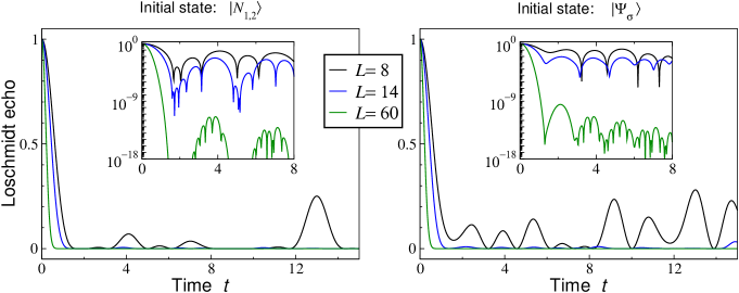
Figure 7: Loschimdt echoes in open chains of sizes $L=8,14,60$ corresponding to the Néel initial state $\ket{N_{1,2}}$ (left), see Eq. (42) and to the initial state $\ket{\Psi_{\sigma}}$ (right), see Eq. (45). For the two smaller sizes, a comparison with Loschmidt echoes numerically calculated by means of exact diagonalization shows exact agreement with the derived closed formulas.

IV.5 Application: time-dependent two-point correlation functions

We now provide a second application of the results on overlap distributions in Sec. IV.2 for the quench $\Delta_{i}=\infty\to\Delta_{f}=0$. We will compute the full time-dependence of finite distance two-point correlation functions after such a quench. For simplicity we will restrict to the periodic chain and list results which are derived in the large-$L$ limit. We provide only a skeleton outline of the derivation, pointing out how the selection rules are used.

The time evolution occurs under the $\Delta=0$ Hamiltonian $H_{\text{xx}}$. The equal-time two-point correlators are defined as

$$G_{\Psi_{0}}^{zz}(j,j+n;t) =\langle\Psi_{0}|\mathrm{e}^{\mathrm{i}tH_{\textnormal{xx}}}S_{j}^{z}S_{j+n}^{z}\mathrm{e}^{-\mathrm{i}tH_{\textnormal{xx}}}|\Psi_{0}\rangle\,,$$ (46)

$$G_{\Psi_{0}}^{+-}(j,j+n;t) =\langle\Psi_{0}|\mathrm{e}^{\mathrm{i}tH_{\textnormal{xx}}}S_{j}^{+}S_{j+n}^{-}\mathrm{e}^{-\mathrm{i}tH_{\textnormal{xx}}}|\Psi_{0}\rangle\,.$$ (47)

We refer to them as the longitudinal and transverse two-point correlators, respectively. We consider as initial state $|\Psi_{0}\rangle$ the four different cases $|\Psi_{+}\rangle=(|N_{1}\rangle+|N_{2}\rangle)/\sqrt{2}$, $|\Psi_{-}\rangle=(|N_{1}\rangle-|N_{2}\rangle)/\sqrt{2}$ and the two Néel states $|N_{1}\rangle$ and $|N_{2}\rangle$ themselves. Since the state $|\Psi_{\sigma}\rangle$ is an eigenstate of the translation operator $\hat{T}$, the two-point correlators only depend on the distance between the two points, $G_{\Psi_{\sigma}}^{zz,+-}(j,j+n;t)=G_{\Psi_{\sigma}}^{zz,+-}(n;t)=\frac{1}{L}\sum_{j=1}^{L}G_{\Psi_{\sigma}}^{zz,+-}(j,j+n;t)$. Applying the Jordan Wigner mapping (10) we obtain

$$G_{\Psi_{0}}^{zz}(n;t) =\frac{1}{L}\sum_{j=1}^{L}\langle\sigma_{j}^{z}\sigma_{j+n}^{z}\rangle=\frac{1}{L}\sum_{j=1}^{L}\langle\left(c_{j}^{{\dagger}}c_{j}^{\phantom{{\dagger}}}-\frac{1}{2}\right)\left(c_{j+n}^{{\dagger}}c_{j+n}^{\phantom{{\dagger}}}-\frac{1}{2}\right)\rangle=\frac{1}{L}\sum_{j=1}^{L}\langle c_{j}^{{\dagger}}c_{j}^{\phantom{{\dagger}}}c_{j+n}^{{\dagger}}c_{j+n}^{\phantom{{\dagger}}}\rangle-\frac{1}{4}$$ (48)

$$G_{\Psi_{0}}^{+-}(n;t) =\frac{1}{L}\sum_{j=1}^{L}\langle c_{j}^{{\dagger}}\left[\prod_{m=1}^{n-1}(1-2c_{j+m}^{{\dagger}}c_{j+m}^{\phantom{{\dagger}}})\right]c_{j+n}^{\phantom{{\dagger}}}\rangle\,,$$ (49)

where from now on the time dependence is implicit, i.e., the expectation values are taken between the time evolved states, $\braket{\cdot}=\braket{\Psi(t)}{\cdot}{\Psi(t)}$ with $\ket{\Psi(t)}=\mathrm{e}^{-\mathrm{i}Ht}\ket{\Psi_{0}}$. In the first line we used that the initial state $|\Psi_{0}\rangle$ lies in the zero magnetization sector and therefore $\frac{1}{L}\sum_{j=1}^{L}\langle c_{j}^{{\dagger}}c_{j}^{\phantom{{\dagger}}}\rangle=1/2$ for all times $t$. In the second line we wrote the ‘Jordan-Wigner string’ operators as $\mathrm{e}^{\mathrm{i}\pi c_{j}^{{\dagger}}c_{j}^{\phantom{{\dagger}}}}=1-2c_{j}^{{\dagger}}c_{j}^{\phantom{{\dagger}}}$, which can be written as

$$1-2c_{j}^{{\dagger}}c_{j}^{\phantom{{\dagger}}}=1-\frac{2}{L}\sum_{p}\tilde{c}_{p}^{{\dagger}}\tilde{c}_{p}^{\phantom{{\dagger}}}-\frac{2}{L}\sum_{\begin{subarray}{c}p,q\\ p\neq q\end{subarray}}\mathrm{e}^{-\mathrm{i}(p-q)j}\tilde{c}_{p}^{{\dagger}}\tilde{c}_{q}^{\phantom{{\dagger}}}\,.$$ (50)

It turns out that the first two terms cancel up to order $1/L$, so that the last term dominates in the large $L$ limit. Thus, the transverse correlator will involve correlators of products like $\left[\prod_{m=1}^{n}c_{p_{m}}^{{\dagger}}\right]\left[\prod_{m=1}^{n}c_{q_{m}}^{\phantom{{\dagger}}}\right]$, where $\{p_{m}\}$ and $\{q_{m}\}$ are sets of $n$ distinct single-particle momenta. As an example, the correlator $G_{\Psi_{\sigma}}^{+-}(n;t)$ is a momentum sum over products of phase factors, which can be rewritten as

$$\langle\Psi_{\sigma}|\left[\prod_{m=1}^{n}c_{p_{m}}^{{\dagger}}\right]\left[\prod_{m=1}^{n}c_{p_{A(m)+\pi}}^{\phantom{{\dagger}}}\right]|\Psi_{\sigma}\rangle =\sum_{\{k\},\{k^{\prime}\}}\langle\Psi_{\sigma}|\{k\}\rangle\langle\{k^{\prime}\}|\Psi_{\sigma}\rangle\;\;\langle\{k^{\prime}\}|\left[\prod_{m=1}^{n}c_{p_{m}}^{{\dagger}}\right]\left[\prod_{m=1}^{n}c_{q_{m}}^{\phantom{{\dagger}}}\right]|\{k\}\rangle$$

$$=(-1)^{\frac{n(n-1)}{2}}\left(\frac{1+(-1)^{n}}{2}\right)\frac{(-1)^{|A|}}{2^{n}}\,,$$ (51)

The second line has been obtained using the selection rules of Sec. IV.2. Since $n$ momenta of the eigenstates $|\{k_{\alpha}\}_{\alpha=1}^{L/2}\rangle$ that obey condition (29) are fixed, there are $\frac{1}{2}\sum_{j=0}^{L/2-n}\binom{L/2-n}{j}=2^{L/2-n-1}$ states with overlap square $2^{-L/2+1}$. This gives the factor $2^{-n}$. The factor $(1+(-1)^{n})/2$ comes from the additional selection rule (‘number of pair flips’) for the total momentum of the eigenstates $|\{k\}\rangle$ and $|\{k^{\prime}\}\rangle$. Hence, the transverse two-point correlator at points $j$ and $j+n$ is only nonzero for $n$ even. Here, $A$ is the mapping matrix from the set $\{p_{m}\}$ to the set $\{q_{m}\}$, given by an element of the symmetric group $\mathcal{S}^{n}$. The factor $(-1)^{|A|}$ implies that the result is a determinant. Carrying all factors and simplifying, we eventually obtain ($t\geq 0$)

$$\hskip 113.81102ptG_{\Psi_{\sigma}}^{+-}(n;t) =\frac{1}{2}\det\nolimits_{n}\Big{(}\tilde{J}_{m-m^{\prime}-1}(2t)\Big{)} \text{for $n$ even}\,,\hskip 113.81102pt$$ (52)

$$\hskip 113.81102ptG_{\Psi_{\sigma}}^{+-}(n;t) =0 \text{for $n$ odd}\,.\hskip 113.81102pt$$ (53)

Here, we have defined the quantity

$$\tilde{J}_{m}(2t)=\frac{(-\mathrm{i})^{m}}{L}\sum_{j=1}^{L}\mathrm{e}^{2\mathrm{i}t\cos(p_{j})-\mathrm{i}mp_{j}}\,.$$ (54)

Similarly, one obtains for the Néel states themselves

$$G_{N_{a}}^{+-}(j,j+n;t)=\frac{(-1)^{n(j+a-1)}}{2\mathrm{i}}\det\nolimits_{n}\Big{(}\tilde{J}_{m-m^{\prime}-1}(2t)\Big{)}\,.$$ (55)

In the derivation of the formulas for $G_{\Psi_{0}}^{+-}$ some $1/L$ terms were dropped. However, we have found that formulas (52) and (53) for $G_{\Psi_{\sigma}}^{+-}(n;t)$ are exact for $n=2,4$ and for any finite even $L$.

The longitudinal correlators are simpler to derive, since they have no Jordan-Wigner strings. The result is

$$G_{\Psi_{0}}^{zz}(n;t)=\frac{1}{4}\Big{(}\delta_{n,0}-\tilde{J}_{n}^{2}(2t)+(-1)^{n}\tilde{J}_{0}^{2}(2t)\Big{)}$$ (56)

for all four initial states $|\Psi_{0}\rangle=\ket{\Psi_{\pm}},\ket{N_{1,2}}$.

In the thermodynamic limit, the summation in Eq. (54) becomes the integral that defines the $m$-th order Bessel function,

$$\tilde{J}_{m}(2t)\xrightarrow{L\to\infty}J_{m}(2t)\,.$$ (57)

Thus, the above formulas for $G_{\Psi_{0}}^{+-}$ and $G_{\Psi_{0}}^{zz}$ are also valid in the thermodynamic limit, with the substitution $\tilde{J}_{m}\to J_{m}$. Previously, Ref. 2010_Barmettler_NewJPhys_12_055017 presented (connected versions of) longitudinal correlators in the thermodynamic limit. To the best of our knowledge, the determinant formulas for the more involved transverse correlators have not appeared previously.

V Quenches from $\Delta_{i}=\infty$ to $\Delta_{f}\ll 1$: perturbative treatment of the splitting

Quenches from the initial state $\ket{\Psi_{\sigma}}$ ($\Delta_{i}=\infty$) to small but nonzero values of $\Delta_{f}$ display a ‘splitting’ of the overlap distribution, as discussed in Sec. III.2 and shown in Figs. 2(a,b). In this section, we will use first order perturbation theory in $\Delta_{f}$ to characterize this splitting.

V.1 First order perturbation expansion

For the final Hamiltonian $H=H_{\textnormal{xx}}+\Delta_{f}H_{\textnormal{z}}$, we consider $\Delta_{f}H_{\textnormal{z}}$ as a perturbative potential $V$. Unfortunately, the unperturbed Hamiltonian $H_{\textnormal{xx}}$ is highly degenerate. In particular, among the states which obey the selection rules, there are many which are degenerate. Hence, a full calculation requires the use of degenerate perturbation theory for many of the eigenstates. However, our purpose here is to provide a basic understanding of the splitting and the general form of the overlap distribution for small nonzero $\Delta_{f}$. Hence, it will suffice to concentrate on those states which have non-degenerate energy eigenvalues, and use the much simpler non-degenerate perturbation theory. We will show that this treatment recovers the main features observed numerically.

For the sake of simplicity we consider a periodic chain with $L/2$ even, which means that in the zero magnetization sector there is an even number $N=L/2$ of fermions in the system. All the calculations can be trivially extended to the odd particle case. In terms of the Jordan-Wigner fermions of Eq. (10), the perturbative potential $V=\Delta_{f}H_{\textnormal{z}}$ can be written as

$$V=\Delta_{f}\sum_{j=1}^{L}\left(n_{j}-\frac{1}{2}\right)\left(n_{j+1}-\frac{1}{2}\right)=\Delta_{f}\sum_{j=1}^{L}\left(n_{j}n_{j+1}-\frac{1}{2}(n_{j}+n_{j+1})+\frac{1}{4}\right)\,,$$ (58)

where $n_{j}=c_{j}^{\dagger}c_{j}^{\phantom{{\dagger}}}$. We can drop the constant term and the terms proportional to the particle number $\hat{N}=\sum_{j=1}^{L}n_{j}$ since they represent just shifts of the energy and are irrelevant for a perturbative expansion. Using again momentum operators defined in Eq. (11) the only relevant contribution can be written as

$$\sum_{j=1}^{L}n_{j}n_{j+1}=\frac{1}{L^{2}}\sum_{j=1}^{L}\sum_{p,q,r,s}\mathrm{e}^{-\mathrm{i}(p-q+r-s)j}\mathrm{e}^{-\mathrm{i}(r-s)}\tilde{c}_{p}^{\dagger}\tilde{c}_{q}^{\phantom{{\dagger}}}\tilde{c}_{r}^{\dagger}\tilde{c}_{s}^{\phantom{{\dagger}}}\,.$$ (59)

Carrying out the sum over the spatial indices we find the condition $q+s=p+r$, which is nothing but the momentum conservation. After these considerations we can rewrite the perturbative potential for the periodic chain as

$$V=\frac{\Delta_{f}}{L}\sum_{p,q,r}\mathrm{e}^{\mathrm{i}(p-q)}\tilde{c}_{p}^{\dagger}\tilde{c}_{q}^{\phantom{{\dagger}}}\tilde{c}_{r}^{\dagger}\tilde{c}_{p-q+r}^{\phantom{{\dagger}}}\,.$$ (60)

Let us now formally write the expression for the corrected overlap. Given $|\Phi\rangle$ the ‘corrected eigenstate’ with $\lim_{\Delta_{f}\to 0}|\Phi\rangle=|\{k_{\alpha}\}_{\alpha=1}^{L/2}\rangle$, the latter being an eigenstate of the XX chain that obeys the selection rules (‘pair condition’ (29) and zero total momentum), we obtain

$$\langle\Psi_{\sigma}|\Phi\rangle=\sqrt{2}\left(\frac{1}{L}\right)^{L/4}\Big{(}\det_{1\leq j,\alpha\leq L/2}\left(\mathrm{e}^{2\mathrm{i}k_{\alpha}j}\Big{)}+\sum_{|\{k^{\prime}\}\rangle}\frac{\langle\{k\}|V|\{k^{\prime}\}\rangle}{E_{k}-E_{k^{\prime}}}\det_{1\leq j,\alpha\leq L/2}\Big{(}\mathrm{e}^{2\mathrm{i}k^{\prime}_{\alpha}j}\Big{)}\right)\,,$$ (61)

where the states $|\{k\}\rangle=|\{k_{\alpha}\}_{\alpha=1}^{L/2}\rangle$ and $|\{k^{\prime}\}\rangle=|\{k^{\prime}_{\alpha}\}_{\alpha=1}^{L/2}\rangle$ are eigenstates of the free fermionic Hamiltonian. Here, we only choose states $|\{k\}\rangle$ for which the energy value $E=\sum_{\alpha=1}^{L/2}\cos(k_{\alpha})$ is non-degenerate, such that the energy difference in the denominator is never zero. Normalizing with $\langle\Psi_{\sigma}|\{k\}\rangle$ we obtain

$$\left|\frac{\langle\Psi_{\sigma}|\Phi\rangle}{\langle\Psi_{\sigma}|\{k\}\rangle}\right|=1-{\sum_{|\{k^{\prime}\}\rangle}}^{\prime}\frac{|\langle\{k\}|V|\{k^{\prime}\}\rangle|}{E_{k}-E_{k^{\prime}}}\,,$$ (62)

where we used that the determinant under the sum is either zero or always given by the same absolute value $|\det_{1\leq j,\alpha\leq L/2}(\mathrm{e}^{2\mathrm{i}k_{\alpha}j})|$. The prime at the sum means that it is restricted to the ‘nonzero overlap states’. The perturbative potential (60) connects states $|\{k\}\rangle$ and $|\{k^{\prime}\}\rangle$ in which just two momenta are exchanged. Due to the selection rule (29) we have that

$$|k_{\alpha}-k^{\prime}_{\alpha}|=\pi\,,\qquad|k_{\beta}-k^{\prime}_{\beta}|=\pi\,.$$ (63)

Therefore, the energy difference in the denominator can be written as

$$E_{k}-E_{k^{\prime}}=\cos(k_{\alpha})+\cos(k_{\beta})-\cos(k^{\prime}_{\alpha})-\cos(k^{\prime}_{\beta})=2\left(\cos(k_{\alpha})+\cos(k_{\beta})\right)\,.$$ (64)

Furthermore, for the numerator, we obtain after a short calculation

$$|\langle\{k\}|V|\{k^{\prime}\}\rangle|=\frac{4\Delta_{f}}{L}\sin^{2}\left(\frac{k_{\alpha}-k_{\beta}}{2}\right)\,.$$ (65)

The sign of $\langle\{k\}|V|\{k^{\prime}\}\rangle$ is fixed by the order of momenta of the states $|\{k\}\rangle$ and $|\{k^{\prime}\}\rangle$. It exactly cancels the sign coming from the determinant that we pulled out of the sum in Eq. (61). The relative minus sign in front of the sum in Eq. (62) is due to the factor $\mathrm{e}^{\mathrm{i}(p-q)}$ in Eq. (60) and comes from the fact that the momenta $k_{\alpha}$, $k_{\beta}$ and $k^{\prime}_{\alpha}$, $k^{\prime}_{\beta}$ differ by $\pm\pi$. In summary, we find

$$\frac{\left|\langle\Psi_{\sigma}|\Phi\rangle\right|-\left|\langle\Psi_{\sigma}|\{k\}\rangle\right|}{\left|\langle\Psi_{\sigma}|\{k\}\rangle\right|}=-\frac{2\Delta_{f}}{L}\sum_{\begin{subarray}{c}\alpha,\beta=1\\ \alpha<\beta\end{subarray}}^{L/2}\frac{\sin^{2}\left(\frac{k_{\alpha}-k_{\beta}}{2}\right)}{\cos(k_{\alpha})+\cos(k_{\beta})}\,.$$ (66)

Follwoing the definition (9) in Sec. III.2, we call the quantity in Eq. (66) the “normalized shift” and the numerator of the left-hand side just the “shift”.

In Fig. 8 we plot the perturbative results (66) for the nonzero overlaps for $\Delta_{f}=0.01$ and $L=48$. (We plot the predictions for actual overlaps instead of the normalized shifts.) The perturbative treatment only covers non-degenerate states. Hence, a quantitative comparison with the numerical data of Fig. 2(a) is not appropriate. However, non-degenerate perturbation theory clearly reproduces the main features of the data. Figure 8 shows the overall shape to be very similar to that seen in the inset to Fig. 2(a), with two branches each having an overall upward slope. The perturbative approach explains the shift being proportional to $\Delta_{f}$ (by providing a non-vanishing contribution at first order in $\Delta_{f}$, see above). In addition, we will show in the subsection below that the result (66) implies that the smallest and largest normalized shifts grow linearly with $L$, so that the normalized average branch shifts grow linearly with $L$, as found numerically, see Fig. 2(b).

The perturbative prediction in Fig. 8 also shows some substructures, e.g., each branch is futher split (recursively) into sub-branches. It is unclear whether such substructures might survive when the degenerate states are taken into account, or when higher-order corrections are included. In addition, substructures in the XXZ spectrum are often heavily determined by boundary conditions 2010_Haque_PRA_82_012108 ; 2014_Sharma_PRA_89_043608 ; 2013_Alba_2013_JStatMech_P10018 . So, they can be expected to be different for periodic and open boundary conditions. A detailed study of such substructures is beyond the scope of the current work.

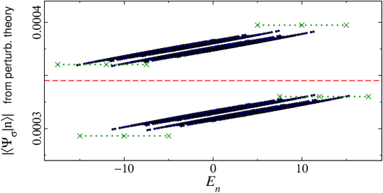
Figure 8: Overlap magnitudes for a quench from $\Delta_{i}=\infty$ to small $\Delta_{f}$, obtained from first-order non-degenerate perturbation theory. The specific values plotted here are for $\Delta_{f}=0.01$ and $L=48$. Only non-degenerate states are included. The dashed line depicts the unperturbed ($\Delta_{f}=0$) value $2^{-L/4+1/2}$. The four horizontal lines (dots and crosses) indicate the extremal values of the shift acoording to Eqs. (67) and (68).

V.2 $L$-dependence of smallest and largest shifts

In order to see how the normalized shift scales with $L$ we compute the sum in Eq. (66) for large system sizes $L$. First of all, we observe that the shift is minimal in absolute value and opposite for the ground state and the highest energy state. For the latter the momenta are uniformly distributed between zero and $\pi/2$ as well as between $3\pi/2$ and $2\pi$ or equivalently, due to the periodicity of the trigonometric functions, between $-\pi/2$ and $\pi/2$. So, $k_{\alpha}=\frac{2\pi}{L}(\alpha-1/2)$ with $-L/4+1\leq\alpha\leq L/4$ and the sum over momenta turns in the thermodynamic limit into an integral from $-\pi/2$ to $\pi/2$ with prefactor $L/(2\pi)$. Therefore, the double sum of the right-hand side of Eq. (66) can be written as

$$\sum_{\begin{subarray}{c}\alpha,\beta=1\\ \alpha<\beta\end{subarray}}^{L/2}\frac{\sin^{2}\left(\frac{k_{\alpha}-k_{\beta}}{2}\right)}{\cos(k_{\alpha})+\cos(k_{\beta})}\;\longrightarrow\;\frac{1}{2}\left(\frac{L}{2\pi}\right)^{2}\int_{-\pi/2}^{\pi/2}\int_{-\pi/2}^{\pi/2}\frac{\sin^{2}\left(\frac{k-q}{2}\right)}{\cos(k)+\cos(q)}dkdq=\frac{L^{2}}{2}\left(\frac{1}{4}-\frac{1}{2\pi}\right)\,.$$ (67)

Together with the small prefactor $2\Delta_{f}/L$ in the perturbative potential (60) this eventually leads to a normalized shift of $-L\Delta_{f}(1/4-1/(2\pi))\approx-0.09085\,L\Delta_{f}$ for the highest energy state and, similarly, $L\Delta_{f}(1/4-1/(2\pi))\approx 0.09085\,L\Delta_{f}$ for the ground state. This means that as we increase the system size $L$ we have to consider smaller and smaller values of $\Delta_{f}$, i.e. $\Delta_{f}\ll 1/L$. Otherwise, we are not in the perturbative regime anymore. To summarize, if we increase the value of the final anisotropy from $\Delta_{f}=0$ to $\Delta_{f}\ll 1/L$, a gap opens in the nontrivial part of the operlap distribution, which we call “splitting” and which scales as $2^{-L/4+1/2}L$ with prefactor $\Delta_{f}(1/2-1/\pi)$, i.e. twice the scaling factor of the shift of the ground state.

Furthermore, the largest value of the shift can be easily computed, too. Our numerical investigation shows that the state that belongs to the largest split is basically given by the set of momenta of the highest energy state where the two innermost momenta $\pm\pi/L$ are replaced by the two momenta $\pm(\pi-\pi/L)$. This leads to an additional contribution with respect to the dominating part of the highest energy state, i.e. $L\Delta_{f}(1/(2\pi)-1/4)$, of

$$-\frac{2\Delta_{f}}{L}\cdot 2\sum_{k_{\beta}}\frac{\sin^{2}\left(\frac{\pi}{2}-\frac{\pi}{2L}-\frac{k_{\beta}}{2}\right)}{\cos(\pi-\pi/L)+\cos(k_{\beta})} =-\frac{2\Delta_{f}}{L}\cdot 4\sum_{m=2}^{L/4}\frac{\sin^{2}\left(\frac{\pi}{2}-\frac{\pi}{2L}-\frac{\pi}{2L}(2m-1)\right)}{-\cos(\pi/L)+\cos(\frac{\pi}{2L}(2m-1))}$$

$$\approx\frac{8\Delta_{f}}{L}\sum_{m=2}^{L/4}\frac{1}{1-\frac{\pi^{2}}{2L^{2}}-(1-\frac{\pi^{2}}{2L^{2}}(2m-1)^{2})}=\frac{4L\Delta_{f}}{\pi^{2}}\sum_{m=2}^{L/4}\frac{1}{m(m-1)}\approx\frac{4L\Delta_{f}}{\pi^{2}}\,.$$ (68)

The first factor $2$ in front of the sum comes from the fact that both innermost momenta are replaced, the second factor $2$ from the fact that the remaining momenta $k_{\beta}$ are symmetrically distributed around zero (modulo periodicity of $2\pi$). Hence, the largest shift also scales like $2^{-L/4+1/2}L$, now with the prefactor $\Delta_{f}(4/\pi^{2}+1/(2\pi)-1/4)\approx 0.31444\,\Delta_{f}$.

In Fig. 8, the large-$L$ predictions for maximum and minimum values of the shifted overlaps, Eqs. (67) and (68), are indicated with horizontal dotted/crossed lines.

VI Quenches from $\Delta_{i}\gg 1$ to $\Delta_{f}=0$: analytical results

In this section we use a perturbative approach to explain one of the features of the overlap distribution that can be observed in the quench protocol from $\Delta_{i}$ large but finite to the free fermion point $\Delta_{f}=0$ . As it can be seen in Fig. 5, the nontrivial part of the overlap distribution is rather smooth as a function of $E_{n}$, and decreases roughly linearly with $E_{n}$. The slope increases with decreasing $\Delta_{i}$. This behavior is in sharp contrast to the splitting structures of the $\Delta_{i}=\infty\to\Delta_{f}\ll 1$ case. In the following we will use perturbation theory in $1/\Delta_{i}$ to show that the normalized shift is proportional to $E_{n}$ at first order (for periodic chains), which explains the smooth behavior of the $|c_{n}|$’s as a function of $E_{n}$. We will also compute the quadratic correction by making use of second order perturbation theory.

For simplicity we consider a periodic chain. In the case of an open chain the main steps of the following calculation can be similarly performed, but there are complications because of the edges. The initial state $\ket{\Psi_{0}}$, which is the ground state at large but finite $\Delta_{i}$, is adiabatically connected to the state $\ket{\Psi_{\sigma}}$, which we have used as the initial state for $\Delta_{i}=\infty$:

$$\lim_{\Delta_{i}\to\infty}\ket{\Psi_{0}}=\ket{\Psi_{\sigma}}\qquad\text{with}\quad\sigma=(-1)^{L/2}\,.$$ (69)

In order to make the perturbative calculation mathematically stringent, we divide the initial Hamiltonian (and henceforth all corresponding energies) by $\Delta_{i}$. We consider the second term in

$$H_{i}/\Delta_{i}=\sum_{j=1}^{L}S_{j}^{z}S_{j+1}^{z}+\frac{1}{\Delta_{i}}\sum_{j=1}^{L}\frac{1}{2}\left(S_{j}^{+}S_{j+1}^{-}+S_{j}^{-}S_{j+1}^{+}\right)=H_{\textnormal{z}}+\Delta_{i}^{-1}H_{\text{xx}}$$ (70)

as a small perturbation.

In order to analyze the overlaps $\langle\{k_{\alpha}\}_{\alpha=1}^{L/2}|\Psi_{0}\rangle$, where $|\{k_{\alpha}\}_{\alpha=1}^{L/2}\rangle$ are the eigenstates of the final Hamiltonian with $\Delta_{f}=0$, perturbatively, we expand the ground state $\ket{\Psi_{0}}$ of $H_{i}$ in the small parameter $1/\Delta_{i}$,

$$\ket{\Psi_{0}}=\ket{\Psi_{0}^{(0)}}+\Delta_{i}^{-1}\ket{\Psi_{0}^{(1)}}+\Delta_{i}^{-2}\ket{\Psi_{0}^{(2)}}+\ldots$$ (71)

The zeroth-order (unperturbed) wavefunction is $\ket{\Psi_{0}^{(0)}}=\ket{\Psi_{\sigma}}$.

The energy eigenvalue $E_{\sigma}$ of $\ket{\Psi_{\sigma}}$ is two-fold degenerate at zeroth order and the corresponding other state is simply $\ket{\Psi_{-\sigma}}$. Since the two states $\ket{\Psi_{-\sigma}}$ and $|\Psi_{0}\rangle$ (with $\sigma$ fixed) are both eigenstates of the translation operator with opposite eigenvalues $-\sigma$ and $\sigma$, we deduce $\langle\Psi_{-\sigma}|\Psi_{0}\rangle=0$. This means that $\ket{\Psi_{-\sigma}}$ does not appear in any expansion of $\ket{\Psi_{0}}$. We can therefore apply non-degenerate perturbation theory. Using $\ket{\Psi_{0}^{(0)}}=\ket{\Psi_{\sigma}}$ the higher order corrections read

$$\ket{\Psi_{0}^{(1)}} =\sum_{\ket{n^{(0)}}\neq\ket{\Psi_{\pm\sigma}}}\ket{n^{(0)}}\frac{\bra{n^{(0)}}H_{\text{xx}}\ket{\Psi_{\sigma}}}{E_{\sigma}-E_{n}^{(0)}}\,,$$ (72)

$$\ket{\Psi_{0}^{(2)}} =\sum_{\ket{m^{(0)}},\ket{n^{(0)}}\neq\ket{\Psi_{\pm\sigma}}}\ket{m^{(0)}}\frac{\bra{m^{(0)}}H_{\text{xx}}\ket{n^{(0)}}}{E_{\sigma}-E_{m}^{(0)}}\frac{\bra{n^{(0)}}H_{\text{xx}}\ket{\Psi_{\sigma}}}{E_{\sigma}-E_{n}^{(0)}}$$

$$\quad-\sum_{\ket{n^{(0)}}\neq\ket{\Psi_{\pm\sigma}}}\ket{n^{(0)}}\frac{\bra{n^{(0)}}H_{\text{xx}}\ket{\Psi_{\sigma}}\bra{\Psi_{\sigma}}H_{\text{xx}}\ket{\Psi_{\sigma}}}{(E_{\sigma}-E_{n}^{(0)})^{2}}\;-\;\frac{1}{2}\ket{\Psi_{\sigma}}\sum_{\ket{n^{(0)}}\neq\ket{\Psi_{\pm\sigma}}}\frac{|\bra{n^{(0)}}H_{\text{xx}}\ket{\Psi_{\sigma}}|^{2}}{(E_{\sigma}-E_{n}^{(0)})^{2}}\,,$$ (73)

where $E_{n}^{(0)}$ is the eigenvalue of $H_{\text{z}}$ with eigenstate $\ket{n^{(0)}}$.

We first compute the matrix elements in the numerator of Eq. (72):

$$\bra{n^{(0)}}H_{\text{xx}}\ket{\Psi_{\sigma}}=\frac{1}{\sqrt{2}}\bra{n^{(0)}}\sum_{j=1}^{L}\frac{1}{2}\left(S_{j}^{+}S_{j+1}^{-}+S_{j}^{-}S_{j+1}^{+}\right)\left(\ket{N_{1}}+\sigma\ket{N_{1}}\right)=\frac{1}{2\sqrt{2}}\left(\delta_{\ket{n^{(0)}}\in S_{1}}+\sigma\delta_{\ket{n^{(0)}}\in S_{2}}\right)\,,$$ (74)

where $S_{1,2}$ are the spaces spanned by the states $\ket{s_{j}^{(1,2)}}=(S_{j}^{+}S_{j+1}^{-}+S_{j}^{-}S_{j+1}^{+})\ket{N_{1,2}}$, $j=1,\ldots,L$, i.e., the space spanned by the spin configurations obtained via a single neighboring spin pair flip from a Néel state. The energies $E_{n}^{(0)}$ are all the same, independent of the choice of $\ket{n^{(0)}}\in S_{1,2}$ and given by $E_{n}^{(0)}=-L/4+1$. Therefore, $E_{\sigma}-E_{n}^{(0)}=-1$ for all $\ket{n^{(0)}}\in S_{1,2}$ and, henceforth,

$$\ket{\Psi_{0}^{(1)}}=-\frac{1}{\sqrt{2}}\left(\frac{1}{2}\sum_{\ket{n^{(0)}}\in S_{1}}\ket{n^{(0)}}+\sigma\frac{1}{2}\sum_{\ket{n^{(0)}}\in S_{2}}\ket{n^{(0)}}\right)=-H_{\textnormal{xx}}\ket{\Psi_{\sigma}}\,.$$ (75)

Thus, the first-order term is obtained by application of $H_{\textnormal{xx}}$ on the initial state (a similar trick was used in Ref. 2014_Luitz_JStatMech_P08007 ).

Using that the states $|\{k\}\rangle=|\{k_{\alpha}\}_{\alpha=1}^{L/2}\rangle$ are eigenstates of the Hamiltonian $H_{\textnormal{xx}}$ with energy $E_{k}$ we obtain up to first order

$$\left|\frac{\langle\{k\}|\Psi_{0}\rangle}{\langle\{k\}|\Psi_{\sigma}\rangle}\right|=1-\frac{E_{k}}{\Delta_{i}}\,.$$ (76)

The second order term is a bit more involved. The first term in Eq. (73) can be computed as

$$\sum_{\ket{m^{(0)}},\ket{n^{(0)}}\neq\ket{\Psi_{\pm\sigma}}}\ket{m^{(0)}}\frac{\bra{m^{(0)}}H_{\text{xx}}\ket{n^{(0)}}}{E_{\sigma}-E_{m}^{(0)}}\frac{\bra{n^{(0)}}H_{\text{xx}}\ket{\Psi_{\sigma}}}{E_{\sigma}-E_{n}^{(0)}}\\ =\;-\sum_{\ket{m^{(0)}}\neq\ket{\Psi_{\pm\sigma}}}\sum_{\ket{n^{(0)}}}\ket{m^{(0)}}\frac{\bra{m^{(0)}}H_{\text{xx}}\ket{n^{(0)}}}{E_{\sigma}-E_{m}^{(0)}}\frac{\delta_{\ket{n^{(0)}}\in S_{1}}+\sigma\delta_{\ket{n^{(0)}}\in S_{2}}}{2\sqrt{2}}\,.$$ (77)

For each fixed state $\ket{n^{(0)}}\in S_{1}\cup S_{2}$ there are of order $L^{2}$ many terms for which the flipped spins do not connect to each other and for which the energy difference is simply $E_{\sigma}-E_{m}^{(0)}=-2$. In contrast, there are only of order $L$ many terms for which the energy difference is not given by this value. We drop these terms because they are subleading in $L$. Since the second and the third term in Eq. (73) are also negligible with respect to the leading contribution, we obtain

$$\ket{\Psi_{0}^{(2)}}=-\frac{1}{2}(H_{\textnormal{xx}})^{2}\ket{\Psi_{\sigma}}\,.$$ (78)

The normalized overlap therefore reads, up to second order in $1/\Delta_{i}$ and by neglecting the $1/L$ contributions,

$$\left|\frac{\langle\{k\}|\Psi_{0}\rangle}{\langle\{k\}|\Psi_{\sigma}\rangle}\right|=1-\frac{E_{k}}{\Delta_{i}}+\frac{1}{2}\left(\frac{E_{k}}{\Delta_{i}}\right)^{2}-\ldots\,.$$ (79)

This provides a second order correction for the nontrivial part of the overlap distribution in the quench protocol from $\Delta_{i}\gg 1$ to $\Delta_{f}=0$.

Note that the energy $E_{k}$ is extensive and bounded by $|E_{k}|\leq L/\pi$. So, if the condition $L/\pi\ll\Delta_{i}$ is fulfilled, we expect the perturbation series to converge. The data for open chains from numerical exact diagonalization, see Fig. 5, is described reasonably well by the large-$L$ perturbative results derived in this section for periodic chains.

VII Conclusions

Motivated by the observation that the overlap distribution is important for many aspects of quench dynamics, in this work we have considered a prominent paradigm model, the XXZ chain, and undertaken a systematic study of the properties of the overlap distribution for quenches of the anisotropy parameter $\Delta$. Using numerical exact diagonalization, we have provided a broad overview of the features of the overlap distribution, for quenches from various values $\Delta_{i}$ to various values of $\Delta_{f}$.

In particular, we have thoroughly analyzed the quench from $\Delta_{i}=\infty$ to $\Delta_{f}=0$, i.e., when the initial state is of the form (8) (combination of Néel states) and the post-quench Hamiltonian is described by a free-fermion theory through Jordan-Wigner transformation. The overlap distribution in this case has the remarkable feature of being ‘flat’: all nonzero overlaps have the same value. Using the free-fermion structure of the post-quench eigenstates, it was possible to analyze the overlap distribution analytically, to express the overlaps using determinant formulas, and to explicitly calculate their values (see Sec. IV). The states that have nonzero overlap can be chosen using certain ‘selection rules’. One rule arises from the spatial structure of the Néel states, while a second rule arises from the symmetry of the initial state (8), in terms of translation (periodic boundary conditions) or reflection (open boundary conditions). The ‘selection rules’ for the periodic chain have been compared with results that we derived from recently obtained Bethe Ansatz formulas 2014_Pozsgay_JStatMech_P06011 ; 2014_Brockmann_JPA_47_145003 ; 2014_Brockmann_JPA_47_345003 . We found that these rules can be equivalently expressed in terms of adjacent corners of rectangles in the pattern of possible XX Bethe roots. We also provided two example applications of our detailed understanding of the overlap distribution for the $\Delta_{i}=\infty\to\Delta_{f}=0$ quench. Using the selection rules, we were able to provide concise expressions for the Loschmidt echo (return probability) as well as equal-time two-point correlators after the quench. In particular, time-dependent transverse correlators, $\langle{}S_{j}^{+}S_{j+n}^{-}\rangle$, are somewhat nontrivial due to Jordan-Wigner strings. We provide determinant formulas for such correlators, derived by making use of the selection rules.

For quenches from $\Delta_{i}=\infty$ to small $\Delta_{f}>0$, the overlap distribution shows a splitting structure which we analyzed perturbatively (perturbation in $\Delta_{f}$, see Sec. V). For quenches from large $\Delta_{i}\gg 1$ to $\Delta_{f}=0$, the overlap distribution acquires a simple dependence on energy which we analyzed using perturbation theory in $1/\Delta_{i}$, see Sec. VI.

The present work is related in various ways to recent advances in non-equilibrium physics. Many recent publications have provided overlap distributions for specific quenches. This motivates systematic studies like the present one. Using the Bethe Ansatz, formulas are now available 2014_Pozsgay_JStatMech_P06011 ; 2014_Brockmann_JPA_47_145003 ; 2014_Brockmann_JPA_47_345003 for the overlap between Néel states and Bethe eingestates at any $\Delta$. Since the use of these results requires knowledge of the Bethe roots describing all eigenstates, it is technically challenging to explore overlap distributions using this approach. Our numerical overview and detailed explicit analysis of specific cases thus provides specific contexts for these general technical results. Our applications to Loschmidt echoes and correlators can be compared with existing calculations of the Loschmidt echo 2006_Quan_PRL_96_140604 ; 2014_Andraschko_PRB_89_125120 and of longitudinal correlators 2010_Barmettler_NewJPhys_12_055017 ). In contrast to these approaches, we have used the structure of the overlap distribution to derive time-dependent quantities. This has allowed us to obtain some new expressions. Finally, certain overlaps with low energy eigenstates in the gapless phase $|\Delta_{f}|<1$ can be studied using field-theoretical methods. In particular, subleading terms in such overlaps 1991_Affleck_PRL_67_161 ; 2011_Stephan_PRB_84_195128 ; 2012_Bondesan_NuclPhysB_862_553 allow to access universal data about the underlying conformal field theory. Our focus here, in contrast, has been on the full spectrum, not just low-energy physics.

This work opens up many new questions. First of all, the present study is by no means exhaustive. There are features of the overlap distribution in the XXZ chain which remain to be analyzed in detail. For example, the physical nature of the eigenstates which have large overlap for $\Delta_{i}=0$ to $\Delta_{f}$ of order one quenches (or vice versa), are unclear and might deserve further study. Second, in addition to the applications we have provided for the cleanest case ($\Delta_{i}=\infty\to\Delta_{f}=0$). It might be possible to exploit the observations on overlap distributions in other quench protocols (other $\Delta_{i}$ and $\Delta_{f}$) to extract properties of the time dependence of Loschmidt echoes and correlation functions. Finally, it would certainly be interesting to analyze overlap distributions in a series of other models. One could ask, for example, whether integrability plays a general role in determining the features of the overlap distribution.

References

- (1) A. Polkovnikov, K. Sengupta, A. Silva, and M. Vengalattore, Rev. Mod. Phys. 83, 863 (2011).
- (2) J. Eisert, M. Friesdorf, and C. Gogolin, Nature Physics 11, 124 (2015).
- (3) J. Dziarmaga, Adv. Phys. 59, 1063 (2010).
- (4) M. Greiner, O. Mandel, T. W. Hansch, and I. Bloch, Nature 419, 51 (2002).
- (5) T. Kinoshita, T. Wenger, and D. S. Weiss, Nature 440, 900 (2006).
- (6) U. Schneider, L. Hackermüller, J. P. Ronzheimer, S. Will, S. Braun, T. Best, I. Bloch, E. Demler, S. Mandt, D. Rasch, and A. Rosch, Nature Phys. 8, 213 (2012).
- (7) S. Trotzky, Y.-A. Chen, A. Flesch, I. P. McCulloch, U. Schollwöck, J. Eisert, and I. Bloch, Nature 8, 325 (2012).
- (8) S. Hofferberth, I. Lesanovsky, B. Fischer, T. Schumm, and J. Schmiedmayer, Nature 449, 324 (2007).
- (9) M. Cheneau, P. Barmettler, D. Poletti, M. Endres, P. Schauss, T. Fukuhara, C. Gross, I. Bloch, C. Kollath, and S. Kuhr, Nature 481, 484 (2012).
- (10) M. Gring, M. Kuhnert, T. Langen, T. Kitigawa, B. Rauer, M. Schreitl, I. Mazets, D. A. Smith, E. Demler, and J. Schmiedmayer, Science 337, 1318 (2012).
- (11) J. P. Ronzheimer, M. Schreiber, S. Braun, S. S. Hodgman, S. Langer, I. P. McCulloch, F. Heidrich-Meisner, I. Bloch, and U. Schneider, Phys. Rev. Lett. 110, 205301 (2013).
- (12) P. J. Lee, M. Anderlini, B. L. Brown, J. Sebby-Strabley, W. D. Phillips, and J. V. Porto, Phys. Rev. Lett. 99, 020402 (2007).
- (13) S. Palzer, C. Zipkes, C. Sias, and M. Köhl, Phys. Rev. Lett. 103, 150601 (2009).
- (14) S. Trotzky, P. Cheinet, S. Fölling, M. Feld, U. Schnorrberger, A. M. Rey, A. Polkovnikov, E. A. Demler, M. D. Lukin, and I. Bloch, Science 319, 295 (2007).
- (15) C. Jarzynski, Phys. Rev. Lett. 78, 2690 (1997).
- (16) P. Talkner, E. Lutz, and P. Hänggi, Phys. Rev. E 75, 050102 (2007).
- (17) M. Campisi, P. Hänggi, and P. Talkner, Rev. Mod. Phys. 83, 771 (2011).
- (18) A. Silva, Phys Rev. Lett. 101, 120603 (2008).
- (19) B. Dóra, A. Bácsi, and G. Zaránd, Phys. Rev. B 86, 161109(R) (2012).
- (20) Y. E. Shchadilova, P. Ribeiro, and M. Haque, Phys. Rev. Lett. 112, 070601 (2014).
- (21) F. N. C. Paraan and A. Silva, Phys. Rev. E 80, 061130 (2009).
- (22) J. Mossel and J.-S. Caux, New J. Phys. 12, 055028 (2010).
- (23) A. Gambassi and A. Silva, arXiv:1106.2671.
- (24) P. Smacchia and A. Silva, Phys. Rev. Lett. 109, 037202 (2012).
- (25) M. Heyl and S. Kehrein, Phys. Rev. B 85, 155413 (2012).
- (26) M. Heyl and S. Kehrein, Phys. Rev. Lett. 108, 190601 (2012).
- (27) A. Gambassi and A. Silva, Phys. Rev. Lett. 109, 250602 (2012).
- (28) P. Smacchia and A. Silva, Phys. Rev. E 88, 042109 (2013).
- (29) L. Mazzola, G. De Chiara, and M. Paternostro, Phys. Rev. Lett. 110, 230602 (2013).
- (30) R. Dorner, S. R. Clark, L. Heaney, R. Fazio, J. Goold, and V. Vedral, Phys. Rev. Lett. 110, 230601 (2013).
- (31) S. Sotiriadis, A. Gambassi, and A. Silva, Phys. Rev. E 87, 052129 (2013).
- (32) A. Sindona, J. Goold, N. Lo Gullo, and F. Plastina, New J. Phys. 16, 045013 (2014).
- (33) J. Marino and A. Silva, Phys. Rev. B 89, 024303 (2014).
- (34) T. Palmai and S. Sotiriadis, Phys. Rev. E 90, 052102 (2014).
- (35) L. Fusco, S. Pigeon, T. J. G. Apollaro, A. Xuereb, L. Mazzola, M. Campisi, A. Ferraro, M. Paternostro, and G. De Chiara, Phys. Rev. X 4, 031029 (2014).
- (36) A. Dutta, A. Das, and K. Sengupta, Phys. Rev. E 92, 012104 (2015).
- (37) T. Palmai, arXiv:1506.08200.
- (38) B. Pozsgay, J. Stat. Mech. P10028 (2013).
- (39) J.-M. Stéphan and J. Dubail, J. Stat. Mech. P08019 (2011).
- (40) H. T. Quan, Z. Song, X. F. Liu, P. Zanardi, and C. P. Sun, Phys. Rev. Lett. 96, 140604 (2006).
- (41) E. J. Torres-Herrera, M. Vyas, L. F. Santos, New J. Phys. 16, 063010 (2014).
- (42) E. J. Torres-Herrera and L. F. Santos, arXiv:1506.08904.
- (43) E. J. Torres-Herrera and L. F. Santos, Phys. Rev. B 92, 014208 (2015).
- (44) E. J. Torres-Herrera and L. F. Santos, Phys. Rev. A 90, 033623 (2014).
- (45) E. J. Torres-Herrera and L. F. Santos, Phys. Rev. E 89, 062110 (2014).
- (46) E. J. Torres-Herrera and L. F. Santos, Phys. Rev. A 89, 043620 (2014).
- (47) E. J. Torres-Herrera and L. F. Santos, Phys. Rev. E 88, 042121 (2013).
- (48) J. Viti, J.-M. Stéphan, J. Dubail, and M. Haque, arXiv:1507.08132.
- (49) A. De Luca, Phys. Rev. B 90, 081403 (2014).
- (50) L. Campos Venuti and P. Zanardi, Phys. Rev. A 81, 022113 (2010).
- (51) J. Häppölä, G. B. Halász, and A. Hamma, Phys. Rev. A 85, 032114 (2012).
- (52) L. Campos Venuti, N. T. Jacobson, S. Santra, and P. Zanardi, Phys. Rev. Lett. 107, 010403 (2011).
- (53) N. T. Jacobson, L. Campos Venuti, and P. Zanardi, Phys. Rev. A 84, 022115 (2011).
- (54) S. Montes and A. Hamma, Phys. Rev. E 86, 021101 (2012).
- (55) V. Mukherjee, S. Sharma, and A. Dutta, Phys. Rev. B 86, 020301(R) (2012)
- (56) K. Lelas, T. Ševa, H. Buljan, and J. Goold, Phys. Rev. A 86, 033620 (2012).
- (57) J.-M. Stéphan and J. Dubail, J. Stat. Mech. P09002 (2013).
- (58) M. Heyl, and M. Vojta, arXiv:1310.6226.
- (59) R. Vasseur, J. P. Dahlhaus, and J. E. Moore, Phys. Rev. X 4, 041007 (2014).
- (60) R. Sachdeva, T. Nag, A. Agarwal, and A. Dutta, Phys. Rev. B 90, 045421 (2014).
- (61) S. Campbell, M. A. Garcia-March, T. Fogarty, and T. Busch, Phys. Rev. A 90, 013617 (2014).
- (62) D. M. Kennes, V. Meden, and R. Vasseur, Phys. Rev. B 90, 115101 (2014)
- (63) A. Rajak and U. Divakaran, arXiv:1507.00963.
- (64) M. Fagotti, arXiv:1308.0277.
- (65) B. Dóra and F. Pollmann, arXiv:1410.5954.
- (66) B. Dóra, F. Pollmann, J. Fortágh, and G. Zaránd, Phys. Rev. Lett. 111, 046402 (2013).
- (67) F. Andraschko and J. Sirker, Phys. Rev. B 89, 125120 (2014).
- (68) M. Heyl, Phys. Rev. Lett. 113, 205701 (2014).
- (69) J. M. Hickey, S. Genway, and J. P. Garrahan, Phys. Rev. B 89, 054301 (2014).
- (70) J. N. Kriel, C. Karrasch, and S. Kehrein, Phys. Rev. B 90, 125106 (2014).
- (71) S. Vajna and B. Dóra, Phys. Rev. B 91, 155127 (2015).
- (72) S. Vajna and B. Dóra, Phys. Rev. B 89, 161105 (2014).
- (73) M. Schmitt and S. Kehrein, Phys. Rev. B 92, 075114 (2015).
- (74) M. Heyl, A. Polkovnikov, and S. Kehrein, Phys. Rev. Lett. 110, 135704 (2013).
- (75) E. Canovi, P. Werner, and M. Eckstein, Phys. Rev. Lett. 113, 265702 (2014).
- (76) C. Karrasch and D. Schuricht, Phys. Rev. B 87, 195104 (2013).
- (77) M. Rigol, V. Dunjko, and M. Olshanii, Nature 452, 854 (2008).
- (78) M. Srednicki, Phys. Rev. E 50, 888 (1994).
- (79) J. M. Deutsch, Phys. Rev. A 43, 2046 (1991).
- (80) C. Neuenhahn and F. Marquardt, Phys. Rev. E 85, 060101 (2012).
- (81) W. Beugeling, R. Moessner, and M. Haque, Phys. Rev. E 89, 042112 (2014).
- (82) J.-S. Caux and F. H. L. Essler, Phys. Rev. Lett. 110, 257203 (2013).
- (83) J. De Nardis, B. Wouters, M. Brockmann, J.-S. Caux, Phys. Rev. A 89, 033601 (2014).
- (84) B. Wouters, J. De Nardis, M. Brockmann, D. Fioretto, M. Rigol, and J.-S. Caux, Phys. Rev. Lett. 113, 117202 (2014).
- (85) B. Pozsgay, M. Mestyán, M. A. Werner, M. Kormos, G. Zaránd, and G. Takács, Phys. Rev. Lett. 113, 117203 (2014).
- (86) M. Brockmann, B. Wouters, D. Fioretto, J. De Nardis, R. Vlijm, and J.-S. Caux, J. Stat. Mech. P12009 (2014).
- (87) A. De Luca, G. Martelloni, and J. Viti, Phys. Rev. A 91, 021603(R) (2015).
- (88) E. Ilievski, J. De Nardis, B. Wouters, J.-S. Caux, F. H. L. Essler, T. Prosen, arXiv:1507.02993.
- (89) M. Rigol, Phys. Rev. Lett. 112, 170601 (2014).
- (90) M. Rigol, Phys. Rev. E 90, 031301(R) (2014).
- (91) A. C. Cassidy, C. W. Clark, and M. Rigol, Phys. Rev. Lett. 106, 140405 (2011).
- (92) M. Rigol and M. Fitzpatrick, Phys. Rev. A 84, 033640 (2011).
- (93) L. F. Santos, A. Polkovnikov, and M. Rigol, Phys. Rev. Lett. 107, 040601 (2011).
- (94) S. Sorg, L. Vidmar, L. Pollet, and F. Heidrich-Meisner, Phys. Rev. A 90, 033606 (2014).
- (95) M. Rigol, Phys. Rev. A 80, 053607 (2009).
- (96) G. Biroli, C. Kollath, and A. M. Läuchli, Phys. Rev. Lett. 105, 250401 (2010).
- (97) S. Hild, T. Fukuhara, P. Schauß, J. Zeiher, M. Knap, E. Demler, I. Bloch, and C. Gross, Phys. Rev. Lett. 113, 147205 (2014).
- (98) W. Heisenberg, Z. Phys. 49, 619 (1928).
- (99) P. Barmettler, M. Punk, V. Gritsev, E. Demler, and E. Altman, New J. Phys. 12, 055017 (2010).
- (100) M. Collura, P. Calabrese, and F. H. L. Essler, arXiv:1507.03492.
- (101) M. Fagotti, M. Collura, F. H. L. Essler, and P. Calabrese, Phys. Rev. B 89, 125101 (2014).
- (102) W. Liu and N. Andrei, Phys. Rev. Lett. 112, 257204 (2014).
- (103) D. Gobert, C. Kollath, U. Schollwöck, and G. Schütz, Phys. Rev. E 71, 036102 (2005).
- (104) V. Alba and F. Heidrich-Meisner, Phys. Rev. B 90, 075144 (2014).
- (105) T. Sabetta and G. Misguich, Phys. Rev. B 88, 245114 (2013).
- (106) R. Vlijm, M. Ganahl, D. Fioretto, M. Brockmann, M. Haque, H. G. Evertz, and J.-S. Caux, arXiv:1507.08624.
- (107) M. Ganahl, M. Haque, and H. G. Evertz, arXiv:1302.2667.
- (108) A. Wöllert and A. Honecker, Phys. Rev. B 85, 184433 (2012).
- (109) S. Langer, F. Heidrich-Meisner, J. Gemmer, I. P. McCulloch, and U. Schollwöck, Phys. Rev. B 79, 214409 (2009).
- (110) M. Haque, Phys. Rev. A 82, 012108 (2010).
- (111) S. Jesenko and M. Žnidarič, Phys. Rev. B 84, 174438 (2011).
- (112) A. Sharma and M. Haque, Phys. Rev. A 89, 043608 (2014).
- (113) C. Karrasch, J. E. Moore, and F. Heidrich-Meisner, Phys. Rev. B 89, 075139 (2014).
- (114) A. De Luca, J. Viti, L. Mazza, and D. Rossini, Phys. Rev. B 90, 161101 (2014).
- (115) C. Karrasch, R. Ilan, and J. E. Moore, Phys. Rev. B 88, 195129 (2013).
- (116) C. Karrasch, J. H. Bardarson, and J. E. Moore, Phys. Rev. Lett. 108, 227206 (2012).
- (117) S. Langer, M. Heyl, I. P. McCulloch, and F. Heidrich-Meisner, Phys. Rev. B 84, 205115 (2011).
- (118) L. Bonnes, F. H. L. Essler, and A. M. Läuchli, Phys. Rev. Lett. 113, 187203 (2014).
- (119) G. Goldstein and N. Andrei, Phys. Rev. A 90, 043625 (2014).
- (120) V. Alba, K. Saha, and M. Haque, J. Stat. Mech. P10018 (2013).
- (121) V. Alba, Phys. Rev. B 91, 155123 (2015).
- (122) M. Brockmann, J. De Nardis, B. Wouters, and J.-S. Caux, J. Phys. A: Math. Theor. 47, 145003 (2014).
- (123) B. Pozsgay, J. Stat. Mech. P06011 (2014).
- (124) M. Brockmann, J. De Nardis, B. Wouters, and J.-S. Caux, J. Phys. A: Math. Theor. 47, 345003 (2014).
- (125) H. Bethe, Z. Phys. 71, 205 (1931).
- (126) R. J. Baxter, Exactly Solved Models in Statistical Mechanics, London: Academic Press, 1982.
- (127) M. Gaudin, La fonction d’onde de Bethe, Paris: Paris Masson, 1983; English translation by J.-S. Caux, Cambridge: Cambridge Univ. Press, 2014.
- (128) E. K. Sklyanin, J. Phys. A: Math. Gen. 21, 2375 (1988).
- (129) V. E. Korepin, N. M. Bogoliubov, and A. G. Izergin, Quantum Inverse Scattering Method and Correlation Functions, Cambridge: Cambridge Univ. Press, 1993.
- (130) L. Piroli and P. Calabrese, J. Phys. A: Math. Theor. 47, 385003 (2014).
- (131) K. K. Kozlowski and B. Pozsgay, J. Stat. Mech. P05021 (2012).
- (132) O. Tsuchiya, J. Math. Phys. 39, 5946 (1998).
- (133) D. J. Luitz, N. Laflorencie, and F. Alet, J. Stat. Mech. P08007 (2014).
- (134) I. Affleck and A. W. W. Ludwig, Phys. Rev. Lett. 67, 161 (1991).
- (135) J.-M. Stéphan, G. Misguich, and V. Pasquier, Phys. Rev. B 84, 195128 (2011).
- (136) R. Bondesan, J. Dubail, J. L. Jacobsen, and H. Saleur, Nucl. Phys. B 862, 553 (2012).