Single electron yields from semileptonic charm and bottom hadron decays in Au$+$Au collisions at $\sqrt{s_{NN}}=200$ GeV

Abstract

The PHENIX Collaboration at the Relativistic Heavy Ion Collider has measured open heavy flavor production in minimum bias Au$+$Au collisions at $\sqrt{s_{{}_{NN}}}=200$ GeV via the yields of electrons from semileptonic decays of charm and bottom hadrons. Previous heavy flavor electron measurements indicated substantial modification in the momentum distribution of the parent heavy quarks due to the quark-gluon plasma created in these collisions. For the first time, using the PHENIX silicon vertex detector to measure precision displaced tracking, the relative contributions from charm and bottom hadrons to these electrons as a function of transverse momentum are measured in Au$+$Au collisions. We compare the fraction of electrons from bottom hadrons to previously published results extracted from electron-hadron correlations in $p$$+$$p$ collisions at $\sqrt{s_{{}_{NN}}}=200$ GeV and find the fractions to be similar within the large uncertainties on both measurements for $p_{T}>4$ GeV/$c$. We use the bottom electron fractions in Au$+$Au and $p$$+$$p$ along with the previously measured heavy flavor electron $R_{AA}$ to calculate the $R_{AA}$ for electrons from charm and bottom hadron decays separately. We find that electrons from bottom hadron decays are less suppressed than those from charm for the region $3<p_{T}<4$ GeV/$c$.

I Introduction

High-energy heavy ion collisions at the Relativistic Heavy Ion Collider (RHIC) and the Large Hadron Collider (LHC) create matter that is well described as an equilibrated system with initial temperatures in excess of 340–420 MeV Adcox et al. (2005); Adams et al. (2005); Adare et al. (2010a); Romatschke (2010); Heinz and Snellings (2013). In this regime, the matter is understood to be a quark-gluon plasma (QGP) with bound hadronic states no longer in existence as the temperatures far exceed the transition temperature of approximately 155 MeV calculated by lattice quantum chromodynamics (QCD) Bazavov et al. (2014). This QGP follows hydrodynamical flow behavior with extremely small dissipation, characterized by the shear viscosity to entropy density ratio $\eta/s\approx 1/4\pi$ and is thus termed a near-perfect fluid Kovtun et al. (2005); Gyulassy and McLerran (2005); Heinz ; Adcox et al. (2005).

Charm and bottom quarks ($m_{c}\approx 1.3$ GeV/$c^{2}$ and $m_{b}\approx 4.2$ GeV/$c^{2}$) are too heavy to be significantly produced via the interaction of thermal particles in the QGP. Thus the dominant production mechanism is via hard interactions between partons in the incoming nuclei, i.e. interactions that involve large momentum transfer, $q^{2}$. Once produced, these heavy quarks are not destroyed by the strong interaction and thus propagate through the QGP and eventually emerge in heavy flavor hadrons, for example $D$ and $B$ mesons.

Early measurement of heavy flavor electrons from the PHENIX Collaboration in Au$+$Au collisions at RHIC indicated that although the total heavy flavor production scales with the number of binary collisions within uncertainties Adler et al. (2005); Adcox et al. (2002), the momentum distribution of these heavy quarks is significantly modified when compared with that in $p$$+$$p$ collisions Adare et al. (2011, 2007a). These results indicate a large suppression for high-$p_{T}$ $>5$ GeV/$c$ electrons and a substantial elliptic flow for $p_{T}$ $=0.3$–$3.0$ GeV/$c$ electrons from heavy quark decays. Here, and throughout the paper, we use “electrons” to refer to both electrons and positrons. The suppression of the charm quark has since been confirmed through the direct reconstruction of $D$ mesons by the STAR Collaboration Adamczyk et al. (2014). In Pb$+$Pb collisions at the LHC at $\sqrt{s_{{}_{NN}}}$ = 2.76 TeV, similar momentum distribution modifications of heavy flavor electrons and $D$ mesons have been measured Abelev et al. (2014, ). Recently, the CMS experiment has reported first measurements of $B\rightarrow J/\psi$  Chatrchyan et al. and b-jets Chatrchyan et al. (2014) in Pb$+$Pb collisions. In contrast to this suppression pattern found in Au$+$Au collisions, $d$$+$Au and peripheral Cu$+$Cu collisions at $\sqrt{s_{{}_{NN}}}=200$ GeV exhibit an enhancement at intermediate electron $p_{T}$ in the heavy flavor electron spectrum Adare et al. (2014a, 2012) that must be understood in terms of a mechanism that enhances the $p_{T}$ spectrum, e.g. the Cronin effect Antreasyan et al. (1979). That mechanism potentially moderates the large suppression observed in Au$+$Au collisions at $\sqrt{s_{{}_{NN}}}=200$ GeV. It is notable that in central Au$+$Au collisions at $\sqrt{s_{{}_{NN}}}$ = 62 GeV an enhancement is also observed at intermediate $p_{T}$ Adare et al. (2015).

The possibility that charm quarks follow the QGP flow was postulated early on Batsouli et al. (2003), and more detailed Langevin-type calculations with drag and diffusion of these heavy quarks yield a reasonable description of the electron data Moore and Teaney (2005); Cao et al. (2013a); Rapp and van Hees ; van Hees et al. (2008); Gossiaux et al. (2010); Adare et al. (2014b). Many of these theory calculations incorporate radiative and collisional energy loss of the heavy quarks in the QGP that are particularly important at high-$p_{T}$, where QGP flow effects are expected to be sub-dominant. The large suppression of heavy flavor electrons extending up to $p_{T}$ $\approx 9$ GeV/$c$ has been a particular challenge to understand theoretically, in part due to an expected suppression of radiation in the direction of the heavy quarks propagation – often referred to as the “dead-cone” effect Dokshitzer and Kharzeev (2001).

This observation of the high-$p_{T}$ suppression Djordjevic and Djordjevic (2014); Djordjevic (2006) is all the more striking because perturbative QCD (pQCD) calculations indicate a substantial contribution from bottom quark decays for $p_{T}$ $>5$ GeV/$c$ Cacciari et al. (2005). First measurements in $p$$+$$p$ collisions at 200 GeV via electron-hadron correlations confirm this expected bottom contribution to the electrons that increases as a function of $p_{T}$ Adare et al. (2009); Aggarwal et al. (2010). To date, there are no direct measurements at RHIC of the contribution of bottom quarks in Au$+$Au collisions.

For the specific purpose of separating the contributions of charm and bottom quarks at midrapidity, the PHENIX Collaboration has added micro-vertexing capabilities in the form of a silicon vertex tracker (VTX). The different lifetimes and kinematics for charm and bottom hadrons decaying to electrons enables separation of their contributions with measurements of displaced tracks (i.e. the decay electron not pointing back to the collision vertex). In this paper, we report on first results of separated charm and bottom yields via single electrons in minimum bias (MB) Au$+$Au collisions at $\sqrt{s_{{}_{NN}}}=200$ GeV.

II PHENIX Detector

As detailed in Ref. Adcox et al. (2003), the PHENIX detector was originally designed with precision charged particle reconstruction combined with excellent electron identification. In 2011, the VTX was installed thus enabling micro-vertexing capabilities. The dataset utilized in this analysis comprises Au$+$Au collisions at $\sqrt{s_{{}_{NN}}}=200$ GeV.

II.1 Global detectors and MB trigger

A set of global event-characterization detectors are utilized to select Au$+$Au events and eliminate background contributions. Two beam-beam counters (BBC) covering pseudorapidity $3.0<|\eta|<3.9$ and full azimuth are located at $\pm$ 1.44 meters along the beam axis and relative to the nominal beam-beam collision point. Each of the BBCs comprises 64 Čerenkov counters.

Based on the coincidence of the BBCs, Au$+$Au collisions are selected via an online MB trigger, which requires at least two counters on each side of the BBC to fire. The MB sample covers $96\pm 3$% of the total inelastic Au$+$Au cross section as determined by comparison with Monte Carlo Glauber models Miller et al. (2007). The BBC detectors also enable a selection on the $z$-vertex position of the collision as determined by the time-of-flight difference between hits in the two sets of BBC counters. The $z$-vertex resolution of the BBC is approximately $\sigma_{z}=0.6$ cm in central Au$+$Au collisions. A selection within approximately $\pm 12$ cm of the nominal detector center was implemented and $\sim$ 85% of all Au$+$Au collisions within that selection were recorded by the PHENIX high-bandwidth data acquisition system.

II.2 The central arms

Electrons ($e^{+}$ and $e^{-}$) are reconstructed using two central spectrometer arms as shown in Fig. 1(a), each of which covers the pseudorapidity range $|\eta|<0.35$ and with azimuthal angle $\Delta\phi=\pi/2$. The detector configuration of the central arms is the same as in previous PHENIX Collaboration heavy flavor electron publications Adare et al. (2011, 2007a). Charged particle tracks are reconstructed outside of an axial magnetic field using layers of drift chamber (DC) and multi-wire proportional pad chambers (PC). The momentum resolution is $\sigma_{p}/p\simeq$ 0.7% $\oplus$ 0.9% $p$ (GeV/$c$). For central arm charged particle reconstructions the trajectory is only measured for radial positions $r>2.02$ meters, and the momentum vector is calculated by assuming the track originates at the Au$+$Au collision point determined by the BBC detectors and assuming 0 radial distance.

Electron identification is performed by hits in a ring imaging Čerenkov detector (RICH) and a confirming energy deposit in an electromagnetic calorimeter (EMCal). The RICH uses CO₂ gas at atmospheric pressure as a Čerenkov radiator. Electrons and pions begin to radiate in the RICH at $p_{T}$ $>$ 20 MeV/$c$ and $p_{T}$ $>$ 4.9 GeV/$c$, respectively. The EMCal is composed of four sectors in each arm. The bottom two sectors of the east arm are lead-glass and the other six are lead-scintillator. The energy resolution of the EMCal is $\sigma_{E}/E\simeq$ 4.5% $\oplus$ 8.3$/\sqrt{E{\rm(GeV)}}$ and $\sigma_{E}/E\simeq$ 4.3% $\oplus$ 7.7$/\sqrt{E{\rm(GeV)}}$ for lead-scintillator and lead-glass, respectively.

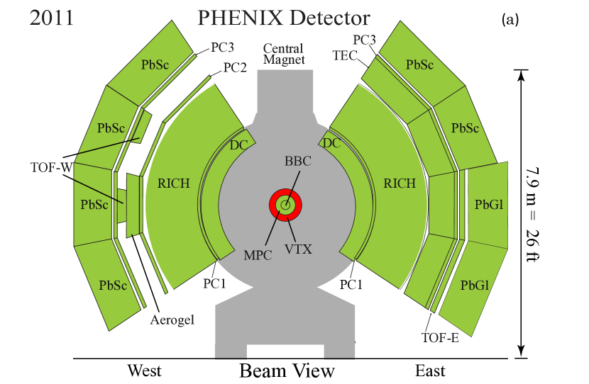
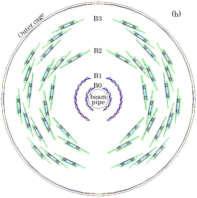
Figure 1: (Color Online) (a) A schematic view of the PHENIX detector configuration for the 2011 run. (b) A schematic view of the VTX detector with the individual ladders shown.

II.3 The VTX detector

In 2011, the central detector was upgraded with the VTX detector as shown in Fig. 1. In addition, a new beryllium beam pipe with 2.16 cm inner diameter and 760 $\mu$m nominal thickness was installed to reduce multiple-scattering before the VTX detector.

The VTX detector Baker et al. ; Nouicer (2013); Kurosawa (2013) consists of four radial layers of silicon detectors as shown in Fig. 1(b). The detector is separated into two arms, each with nominal acceptance $\Delta\phi\approx 0.8\pi$ centered on the acceptance of the outer PHENIX central arm spectrometers. The detector covers pseudorapidity $|\eta|<$ 1.2 for collisions taking place at $z=0$. The VTX can precisely measure the vertex position of a collision within $|z|<10$ cm range of the center of the VTX.

The two inner layers, referred to as B0 and B1, of the VTX detector comprise silicon pixel detectors, as detailed in Ref. Ichimiya et al. (2009). B0 (B1) comprises 10 (20) ladders with a central radial position of 2.6 (5.1) cm. The silicon pixel technology is based on the ALICE1LHCb sensor-readout chip Snoeys et al. (2001), which was developed at CERN. Each ladder is electrically divided into two independent half-ladders. Each ladder comprises four sensor modules mounted on a mechanical support made from carbon-fiber composite. Each sensor module comprises a silicon pixel sensor with a pixel size of 50 $\mu$m($\phi$) $\times$ 425 $\mu$m($z$) bump-bonded with four pixel readout chips. One pixel readout chip reads 256 $(\phi)\times$ 32 $(z)$= 8192 pixels and covers approximately 1.3 cm $(\Delta\phi)\times$ 1.4 cm $(\Delta z)$ of the active area of the sensor. The position resolution is $\sigma_{\phi}$ = 14.4 $\mu$m in the azimuthal direction.

The two outer layers of the VTX detector, referred to as B2 and B3, are constructed using silicon stripixel sensors, as detailed in Ref. Ichimiya et al. (2009). The B2 (B3) layer comprises 16 (24) silicon stripixel ladders at a central radial distance of 11.8 (16.7) cm. The stripixel sensor is a novel silicon sensor, and is a single-sided, N-type, DC-coupled, two-dimensional (2-D) sensitive detector Li et al. (2004); Nouicer et al. (2009). One sensor has an active area of approximately 30 mm $\times$ 60 mm, which is divided into two independent sectors of 30 mm $\times$ 30 mm. Each sector is divided into 384 $\times$ 30 pixels. Each pixel has an effective size of 80 $\mu$m ($\phi$) $\times$ 1000 $\mu$m ($z$), leading to a position resolution of $\sigma_{\phi}$=23 $\mu$m. A pixel comprises two implants (A and B) interleaved such that each of the implants registers half of the charge deposited by ionizing particles. There are 30 A implants along the beam direction, connected to form a 30 mm long X-strip, and 30 B implants are connected with a stereo angle of 80 mrad to form a U-strip. X-strip and U-strip are visualized in Nouicer et al. (2009). When a charged particle hits a pixel, both the X- and the U-strip sharing the pixel register a hit. Thus the hit pixel is determined as the intersection of the two strips. The stripixel sensor is read out with the SVX4 chip developed by a FNAL-LBNL Collaboration Garcia-Sciveres et al. (2003).

The total number of channels in the VTX pixel and stripixel layers is 3.9 million pixels and 0.34 million strips. The compositions of the pixel and strip are illustrated in Ichimiya et al. (2009); Nouicer et al. (2009). The main characteristics of the VTX detector are summarized in Table 1.

Table 1: A summary of the VTX detector. For each layer (B0 to B3), the detector type, the central radius ($r$), ladder length ($l$), sensor thickness ($t$), sensor active area ($\Delta\phi\times\Delta z$), the number of sensors per ladder ($N_{S}$), the number of ladders ($N_{L}$), pixel/strip size in $\phi$ ($\Delta\phi$) and z ($\Delta z$), the number of read-out channels ($N_{ch}$), and the average radiation length including the support and on-board electronics ($X_{0}$) are given.

					sensor active area			pixel/strip size
	type	$r$(cm)	$l$(cm)	$t$ ($\mu$m)	$\Delta\phi$(cm)	$\Delta z$(cm)	$N_{S}$	$N_{L}$	$\Delta\phi$ ($\mu$m)	$\Delta z$ ($\mu$m)	$N_{ch}$	$X_{0}$(%)
B0	pixel	2.6	22.8	200	1.28	5.56	4	10	50	425	$1.3\times 10^{6}$	1.3
B1	pixel	5.1	22.8	200	1.28	5.56	4	20	50	425	$2.6\times 10^{6}$	1.3
B2	stripixel	11.8	31.8	625	3.07	6.00	5	16	80	$3\times 10^{4}$	$1.2\times 10^{5}$	5.2
B3	stripixel	16.7	38.2	625	3.07	6.00	6	24	80	$3\times 10^{4}$	$2.2\times 10^{5}$	5.2

III Analysis

III.1 Overview

The purpose of the analysis is to separate the electrons from charm and bottom hadron decays. The life time of $B$ mesons ($c\tau_{B^{0}}$= 455 $\mu$m, $c\tau_{B^{\pm}}$ = 491 $\mu$m Olive et al. (2014)) is substantially longer than that of $D$ mesons ($c\tau_{D^{0}}$ = 123 $\mu$m, $c\tau_{D^{\pm}}$ = 312 $\mu$m) and the decay kinematics are different. This means that the distribution of values for the distance of closest approach (DCA) of the track to the primary vertex for electrons from bottom decays will be broader than that of electrons from charm decays. There are other sources of electrons, namely Dalitz decays of $\pi^{0}$ and $\eta$, photon conversions, $K_{e3}$ decays, and $J/\psi\rightarrow e^{+}e^{-}$ decays. With the exception of electrons from $K_{e3}$ decays, these background components have DCA distributions narrower than those from charm decay electrons. Thus we can separate $b\rightarrow e$, $c\rightarrow e$ and background electrons via precise measurement of the DCA distribution.

In the first step of the analysis, we select good events where the collision vertex is within the acceptance of the VTX detector, and its function is normal (Sec. III.2). We then reconstruct electrons in the PHENIX central arms (Sec. III.3). The electron tracks are then associated with hits in the VTX detector and their DCA is measured (Sec. III.4). At this point we have the DCA distribution of inclusive electrons that has contributions from heavy flavor ($b\rightarrow e$ and $c\rightarrow e$) and several background components.

The next step is to determine the DCA shape and normalization of all background components (Sec. III.5). They include mis-identified hadrons, background electrons with large DCA caused by high-multiplicity effects, photonic electrons (Dalitz decay electrons, photon conversions), and electrons from $K_{e3}$ and quarkonia decays. The shapes of the DCA distributions of the various background electrons are determined via data driven methods or Monte Carlo simulation. We then determine the normalization of those background electron components in the data (Sec. III.6).

Because the amount of the VTX detector material is substantial (13% of one radiation length) the largest source of background electrons is photon conversion within the VTX. We suppress this background by a conversion veto cut (Sec. III.5.3)

Once the shape and the normalization of all background components are determined and subtracted, we arrive at the DCA distribution of heavy flavor decay electrons that can be described as a sum of $b\rightarrow e$ and $c\rightarrow e$ DCA distributions. The heavy flavor DCA distribution is decomposed by an unfolding method (Sec. III.7).

III.2 Event selection

The data set presented in this analysis is from Au$+$Au collisions at $\sqrt{s_{{}_{NN}}}=200$ GeV recorded in 2011 after the successful commissioning of the VTX detector. As detailed earlier, the MB Au$+$Au data sample was recorded using the BBC trigger sampling $96\pm 3$% of the inelastic Au$+$Au cross section. A number of offline cuts were applied for optimizing the detector acceptance uniformity and data quality as described below. After all cuts, a data sample of 2.4$\times 10^{9}$ Au$+$Au events was analyzed.

III.2.1 z-vertex selection

The acceptance of the PHENIX central arm spectrometers covers collisions with $z$-vertex within $\pm$ 30 cm of the nominal interaction point. The VTX detector is more restricted in $|z|$ acceptance, as the B0 and B1 layers cover only $|z|<11.4$ cm. Thus the BBC trigger selected only events within the narrower vertex range of $|z_{\rm BBC}|<12$ cm. In the offline reconstruction, the tracks reconstructed from VTX information alone are used to reconstruct the Au$+$Au collision vertex with resolution ${\sigma_{z}}=75$ $\mu$m. All Au$+$Au events in the analysis are required to have a $z$-vertex within $\pm$10 cm as reconstructed by the VTX.

III.2.2 Data quality assurance

Due to a number of detector commissioning issues in this first data taking period for the VTX, the data quality varies substantially. Therefore we divide the entire 2011 Au$+$Au data taking period into four periods. The acceptance of the detector changes significantly between these periods.

In addition, several cuts are applied to ensure the quality and the stability of the data. Applying electron identification cuts described in Sec. III.3.2, the electron to hadron ratios were checked for each run, a continuous data taking period typically lasting of order one hour, and three runs out of 547 with ratios outside of 5$\sigma$ from the mean were discarded. The B2 and B3 stripixel layers had an issue in stability of read-out electronics where some of the sensor modules would drop out, resulting in a reduced acceptance within a given run. Additional instabilities also existed in the B0 and B1 pixel layers. Detailed channel by channel maps characterizing dead, hot, and unstable channels were generated for all layers within a given run. These maps were used to mask dead, hot, and unstable channels from the analysis, as well as to define the fiducial area of the VTX in simulations.

During this first year of data taking, the instability of the read-out electronics discussed above caused significant run-to-run variations in the acceptance and efficiency of the detector. It is therefore not possible to reliably calculate the absolute acceptance and efficiency correction while maintaining a large fraction of the total data set statistics. Instead, we report on the relative yields of charm and bottom to total heavy flavor. We have checked that the DCA distributions are consistent between running periods and are not impacted by the changing acceptance. Thus we can measure the shape of the DCA distribution using the entire data set. In the following, we use the shape of the measured DCA distribution only to separate $b\rightarrow e$ and $c\rightarrow e$ components.

III.3 Electron reconstruction in central arms

III.3.1 Track reconstruction

Charged particle tracks are reconstructed using the outer central arm detectors, DC and PC, as detailed in Ref. Adare et al. (2007a). The DC has six types of wire modules stacked radially, named X1, U1, V1, X2, U2, and V2. The X wires run parallel to the beam axis in order to measure the $\phi$-coordinate of the track and the U and V wires have stereo angles varying from 5.4 to 6.0 degrees. Tracks are required to have hits in both the X1 and X2 sections along with uniquely associated hits in the U or V stereo wires and at least one matching PC hit, to reduce mis-reconstructed tracks. The track momentum vector is determined assuming the particle originated at the Au$+$Au collision vertex as reconstructed by the BBC.

III.3.2 Electron identification

Electron candidates are selected by matching tracks with hits in the RICH and energy clusters in the EMCal. The details on the electron selection cuts are given in Ref. Adare et al. (2011). In this analysis we select electron candidates within $1.5<\mbox{$p_{T}$}\ [\mbox{GeV/$c$}]<5.0$, and we briefly describe the cuts in the RICH and EMCal below.

Čerenkov photons from an electron track produce a ring-shaped cluster in the RICH. At least three associated PMT hits are required in the RICH and a ring-shape cut is applied. The center of the ring is required to be within 5 cm of the track projection. The probability that the associated cluster in the EMCal comes from an electromagnetic shower is calculated based on the shower shape. Based on that probability, tracks are selected in a way that maintains high efficiency for electrons while rejecting hadrons. Further, the energy ($E$) in the EMCal is required to match the track determined momentum ($p$). This match is calculated as $dep=(E/p-\mu_{E/p})/\sigma_{E/p}$, where $\mu_{E/p}$ and $\sigma_{E/p}$ are the mean and standard deviation respectively of a Gaussian fit to the $E/p$ distribution, determined as a function of momentum (see Fig. 2). A cut of $dep>-2$ is used to further reject hadrons that have an $E/p$ ratio $<1$, because they do not deposit their full energy in the EMCal.

In high-multiplicity Au$+$Au events there is a significant probability for a random association between the track and hits in the RICH and EMCal. This mis-identified hadron probability is estimated as follows. The $z<0$ and $z>0$ sides of the RICH have their hits swapped in software, and the tracks are re-associated with RICH hits. Because the two longitudinal sides of the RICH are identical, this gives a good estimate of the random hadron background in the electron sample.

The distribution of electron candidates at $p_{T}$ =2.0–2.5 GeV/$c$ for the normalized EMCal energy to track momentum ratio, $dep$ defined above, is shown in Fig. 2. There is a large peak near zero from true electrons as expected and a clear low-side tail from mis-identified hadron. Also shown is the result of the above swap method. The difference between the data and the “swap” distribution (red) is explained as contributions from off-vertex electrons caused by conversions from the outer layer of the VTX and weak decay. In the final accounting for all contributions to the identified-electron DCA distribution, we utilize this swap method to statistically estimate the contribution of mis-identified hadron in each $p_{T}$ selection as detailed in Section III.5.1.

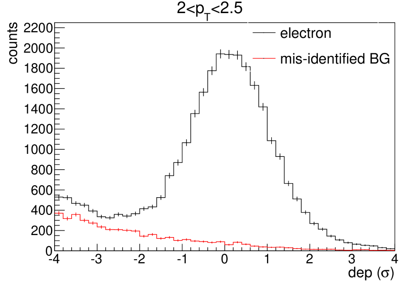
Figure 2: (Color Online) Matching variable between the reconstructed track momentum ($p$) and the energy measured in the EMCal ($E$): $dep=(E/p-\mu_{E/p})/\sigma_{E/p}$. The black distribution is for identified electrons with $p_{T}$ = 2.0–2.5 GeV/$c$, and the red distribution is the estimated contribution from mis-identified electrons via the RICH swap-method.

III.4 DCA measurement with the VTX

Charged particle tracks reconstructed in the central arms must be associated with VTX hits in order to calculate their DCA. Three-dimensional (3-D) hit positions in the 4 layers of VTX are reconstructed. For each collision, the primary vertex is reconstructed by the VTX. Then central arm tracks are associated with hits in the VTX, and VTX-associated tracks are formed. Finally, the DCA between the primary vertex and the VTX-associated tracks are measured.

III.4.1 VTX alignment

In order to achieve good DCA resolution to separate $b\rightarrow e$ and $c\rightarrow e$, alignment of the detector ladders to high precision is required. The detector alignment is accomplished via an iterative procedure of matching outer central arm tracks from the DC and PC to the VTX hits. The procedure is convergent for the position of each ladder. The alignment was repeated each time the detector was repositioned following a service access. The final alignment contribution to the DCA resolution in both $\phi$ and $z$ is a few tens of microns.

III.4.2 VTX hit reconstruction

For layers B0 and B1, clusters of hit pixels are formed by connecting contiguous hit pixels by a recursive clustering algorithm. An average cluster size is 2.6 (6.7) pixels for the pixel (stripixel). The center of the cluster in the local 2-D coordinate system of the sensor is calculated as the hit position.

For B2 and B3 layers, 2D hit points on the sensor are reconstructed from the X-view and the U-view. Hit lines in the X-view (U-view) are formed by clustering contiguous hit X-strips (U-strips) weighted by deposited charges, and then 2D hit points are formed as the intersections of all hit lines in X- and U- views. When one hit line in U-view crosses more than two hit lines in X-view, ghost hits can be formed, because which crossing point is the true hit is ambiguous. These ghost hits increase the number of reconstructed 2D hits approximately by 50% (30%) in B2 (B3) in central Au$+$Au collisions. The ghost hit rate was studied using a full geant3 GEA simulation with the HIJING Wang and Gyulassy (1991) generator as input. However, because the occupancy of the detector at the reconstructed 2D hit point level is low, less than 0.1%, these ghost hits do not cause any significant issue in the analysis.

The positions of all 2-D hits in the VTX are then transferred into the global PHENIX 3-D coordinate system. Correction of the sensor position and orientation, determined by the alignment procedure described in the previous section, is applied in the coordinate transformation. The resulting 3-D hit positions in the global coordinate system are then used in the subsequent analysis.

III.4.3 The primary vertex reconstruction

With the VTX hit information alone, charged particle tracks can be reconstructed only with modest momentum resolution $\delta p/p\approx$ 10% due to the limited magnetic field integrated over the VTX volume and the multiple scattering within the VTX. These tracks can be utilized to determine the collision vertex in three-dimensions ($z_{0}$ along the beam axis, and $x_{0}$,$y_{0}$ in the transverse plane) for each Au$+$Au event under the safe assumption that the majority of particles originate at the collision vertex. This vertex position is called the primary vertex position.

The position resolution of the primary vertex for each direction depends on the sensor pixel and strip sizes, the precision of the detector alignment, and the number of particles used for the primary vertex calculation and their momentum in each event. For MB Au$+$Au collisions, the resolution values are $\sigma_{x}=96$ $\mu$m, ${\sigma_{y}}=43$ $\mu$m, and ${\sigma_{z}}=75$ $\mu$m. The worse resolution in $x$ compared to $y$ is due to the orientation of the two VTX arms. For comparison, the beam profile in the transverse plane is $\sigma^{\rm lumi}_{x}\approx\sigma_{y}^{\rm lumi}\approx 90$ $\mu$m in the 2011 Au$+$Au run.

III.4.4 Association of a central arm track with VTX

Each central arm track is projected from the DC through the magnetic field to the VTX detector. Hits in VTX are then associated with the track using a recursive windowing algorithm as follows.

The association starts from layer B3. VTX hits in that layer that are within a certain ($\Delta\phi\times\Delta z$) window around the track projection are searched. If hits are found in this window, the track is connected to each of the found hits, and then projected inward to the next layer. In this case the search window in the next layer is decreased, because there is much less uncertainty in projection to the next layer. If no hit is found, the layer is skipped, and the track is projected inward to the next layer, keeping the size of the projection window. This process continues until the track reaches layer B0, and a chain of VTX hits that can be associated with the track is formed. The window sizes are momentum dependent and determined from a full geant3 simulation of the detector so that the inefficiency of track reconstruction due to the window size is negligible.

After all possible chains of VTX hits that can be associated with a given central arm track are found by the recursive algorithm, a track model fit is performed for each of these possible chains, and the $\chi^{2}$ of the fit, $\chi^{2}_{\rm vtx}$, is calculated. The effect of multiple scattering in each VTX layer is taken into account in calculation of $\chi^{2}_{\rm vtx}$. Then the best chain is chosen based on the value of $\chi^{2}_{\rm vtx}$ and the number of associated hits. This best chain and its track model are called a VTX-associated track. Note that at most one VTX-associated track is formed from each central arm track.

In this analysis we require that VTX-associated tracks have associated hits in at least the first three layers, i.e. B0, B1, and B2. An additional track requirement is $\chi^{2}_{\rm vtx}/{\rm NDF}<2$ for $p_{T}$ $<2$ GeV/$c$ and $\chi^{2}_{\rm vtx}/{\rm NDF}<3$ for $p_{T}$ $>2$ GeV/$c$, where NDF is the number of degrees of freedom in the track fit.

III.4.5 $\mathrm{DCA}_{T}$ and $\mathrm{DCA}_{L}$

Using the primary vertex position determined above, the DCA of a track is calculated separately in the transverse plane ($\mathrm{DCA}_{T}$) and along the beam axis ($\mathrm{DCA}_{L}$). Because by design the $\mathrm{DCA}_{T}$ has a better resolution than $\mathrm{DCA}_{L}$, we first find $\mathrm{DCA}_{T}$ with a track model of a circle trajectory assuming the uniform magnetic field over the VTX. We define $\mathrm{DCA}_{T}$ as

$$\mbox{$\mathrm{DCA}_{T}$}\equiv L-R,$$ (1)

where $L$ is the distance from the collision vertex to the center of the circle defining the particle trajectory, and $R$ is the radius of the circle as shown in Fig. 3. $\mathrm{DCA}_{L}$ is the distance between the z-coordinate of the point $\mathrm{DCA}_{T}$ found and z-coordinate of the primary vertex.

It is notable that $\mathrm{DCA}_{T}$ has a sign in this definition. The distinction between positive and negative values of $\mathrm{DCA}_{T}$—whether the trajectory is bending towards or away from the primary vertex—is useful since certain background contributions have asymmetric distributions in positive and negative $\mathrm{DCA}_{T}$, as discussed in section III.5. For electrons, the positive side of $\mathrm{DCA}_{T}$ distribution has less background contribution. There is no such positive/negative asymmetry in $\mathrm{DCA}_{L}$.

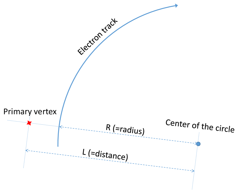
Figure 3: (Color Online) Illustration of the definition of $\mathrm{DCA}_{T}$ $\equiv$ $L$ - $R$ in the transverse plane.

III.4.6 DCA measurement

For each VTX-associated track, the DCA is calculated separately in the radial and longitudinal direction ($\mathrm{DCA}_{T}$ and $\mathrm{DCA}_{L}$) from the track model and the primary vertex position. Shown in Fig. 4 is the resulting $\mathrm{DCA}_{T}$ and $\mathrm{DCA}_{L}$ distributions for all VTX-associated tracks with $p_{T}$ = 2.0–2.5 GeV/$c$. Since the vast majority of charged tracks are hadrons originating at the primary vertex, we observe a large peak around $\mathrm{DCA}_{T}$, $\mathrm{DCA}_{L}$ = 0 that is well fit to a Gaussian distribution where the $\sigma$ represents the $\mathrm{DCA}_{T}$, $\mathrm{DCA}_{L}$ resolution. A selection of $|$$\mathrm{DCA}_{L}$ $|<0.1$ cm is applied to reduce background.

There are broad tails for $|$$\mathrm{DCA}_{T}$ $|>$ 0.03 cm. Monte Carlo simulation shows that the main source of the broad tails is the decay of long lived light hadrons such as $\Lambda$ and $K_{S}^{0}$.

The $\mathrm{DCA}_{T}$ resolution as a function of the track $p_{T}$ is extracted using a Gaussian fit to the peak and is shown in Fig. 4 c). The $\mathrm{DCA}_{T}$ resolution is approximately 75 $\mu$m for the 1.0–1.5 GeV/$c$ bin and decreases with increasing $p_{T}$ as the effect of multiple scattering becomes smaller for higher $p_{T}$. The $\mathrm{DCA}_{T}$ resolution becomes less than 60 $\mu$m for $p_{T}$ $>$ 4 GeV/$c$, where it is limited by the position resolution of the primary vertex.

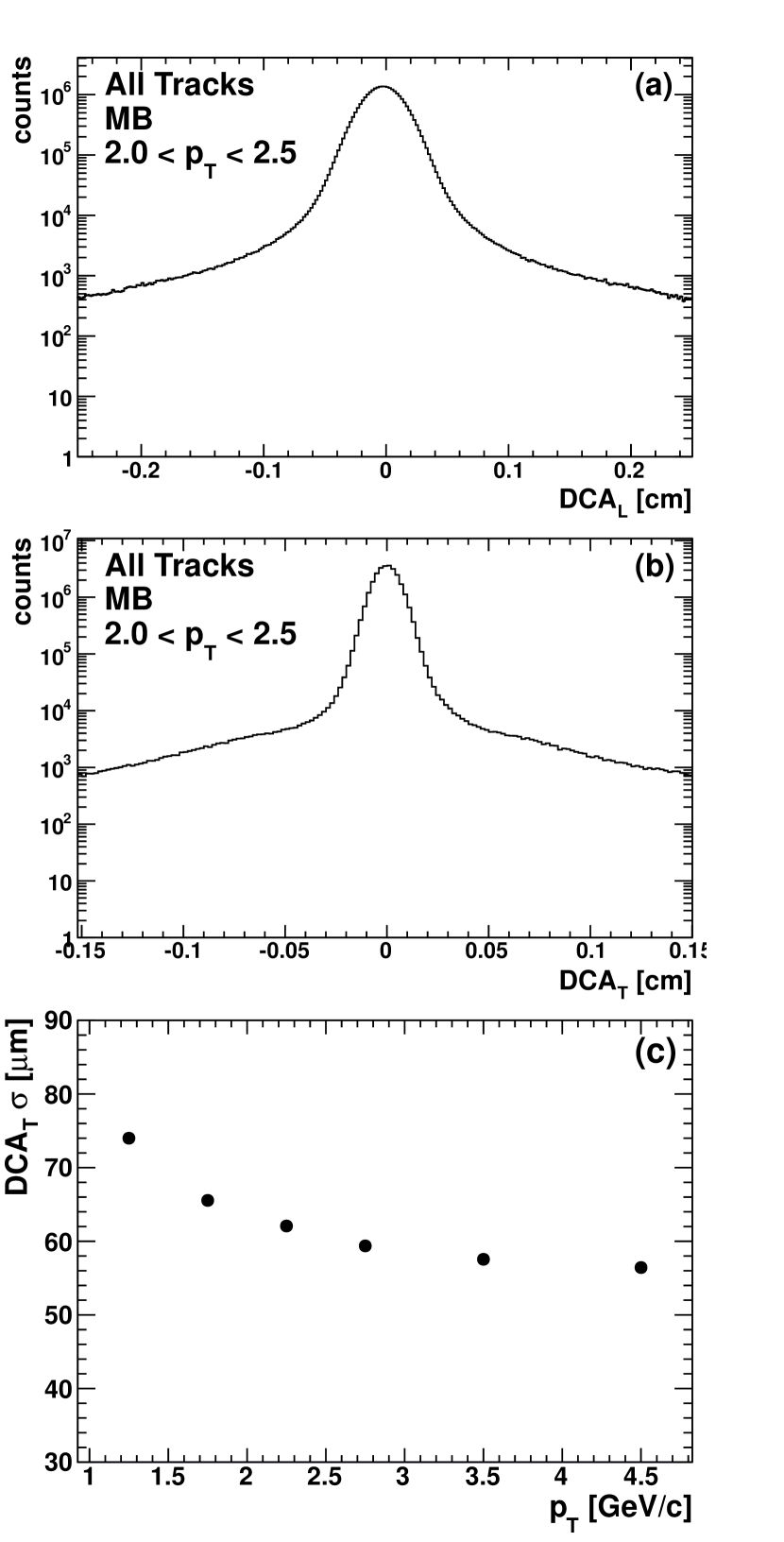
Figure 4: Distance-of-closest-approach distributions for (a) along the beam axis $\mathrm{DCA}_{L}$ and (b) transverse plane $\mathrm{DCA}_{T}$ for all VTX-associated tracks in Au$+$Au at $\sqrt{s_{{}_{NN}}}=200$ GeV in the range $2.0<\mbox{$p_{T}$}\,[{\rm~{}GeV}/c]<2.5$. (c) The $\mathrm{DCA}_{T}$ resolution as a function of $p_{T}$ for all tracks.

We divide the electrons into five $p_{T}$ bins and show the $\mathrm{DCA}_{T}$ distributions for each in Fig. 5. These distributions are in integer-value counts and are not corrected for acceptance and efficiency. The DCA distributions include various background components other than heavy flavor contributions. The background components are also shown in the figure and are discussed in the next section (Section III.5).

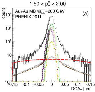
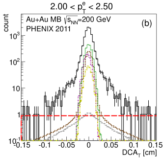
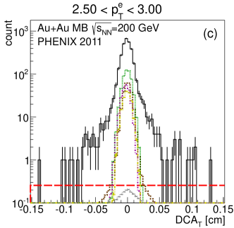
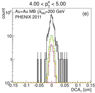
Figure 5: (Color Online) $\mathrm{DCA}_{T}$ distributions for electrons in MB Au$+$Au at $\sqrt{s_{{}_{NN}}}=200$ GeV that pass the reconstruction and conversion veto cut in the indicated five electron-$p_{T}$ selections. Also shown are the normalized contributions for the various background components detailed in Section III.5.

While the $\mathrm{DCA}_{T}$ distributions in Fig. 5 are plotted within $|\mbox{$\mathrm{DCA}_{T}$}|<0.15$ cm, only a $|\mbox{$\mathrm{DCA}_{T}$}|<0.1$ cm is used in the analysis to extract the charm and bottom yield described later. At large $\mathrm{DCA}_{T}$, the distribution is dominated by high-multiplicity background (Sec. III.5.2) and therefore provides little constraint in the extraction of the charm and bottom contributions.

III.5 DCA distribution of Background Components

The sample of candidate electron tracks that pass all the analysis cuts described above contains contributions from a number of sources other than the desired electrons from semi-leptonic decays of charm and bottom hadrons. In order to extract the heavy flavor contributions, all background components must be fully accounted for and their $\mathrm{DCA}_{T}$ shapes as a function of $p_{T}$ incorporated. These background components are listed in the order presented below.

1. Misidentified hadrons

2. High-multiplicity background

3. Photonic electrons

4. Kaon decay electrons

5. Heavy-quarkonia decay electrons

As described in this and the following section, all background components are constrained by PHENIX measurements in Au$+$Au and are fully simulated through a geant3 description of the detector. This method is similar to the cocktail method of background subtraction used in the previous analysis of inclusive heavy flavor electrons Adare et al. (2011).

Next, we describe these background sources and their DCA distributions. The first two components are caused by detector and multiplicity effects. DCA distributions and normalization of these two components are determined by data driven methods, as detailed in this section. The last three components are background electrons that are not the result of semi-leptonic decays of heavy flavor hadrons. Their DCA distributions are determined by Monte Carlo simulation, and their normalization is determined by a bootstrap method described in section III.6. Of those background electrons, photonic electrons are the dominant contribution. We developed a conversion veto cut to suppress this background (III.5.3).

III.5.1 Mis-identified hadron

As detailed in the discussion on electron identification, there is a nonzero contribution from mis-identified electrons. This contribution is modeled via the RICH swap-method described in Section III.3.2. From this swap method, we obtain the probability that a charged hadron is mis-identified as an electron as a function of $p_{T}$. This probability is then applied to the DCA distribution of charged hadrons to obtain the DCA distribution of mis-identified hadrons.

The resulting $\mathrm{DCA}_{T}$ distribution is shown in each panel of Fig. 5. Note that this component is properly normalized automatically. For each $p_{T}$ bin, the DCA distribution of mis-identified prompt hadrons has a narrow Gaussian peak at $\mbox{$\mathrm{DCA}_{T}$}=0$. The broad tails for large $|$$\mathrm{DCA}_{T}$ $|$ are mainly caused by decays of $\Lambda$ and $K_{S}^{0}$. In all $p_{T}$ bins the magnitude of this background is no more than 10% of the data for all $\mathrm{DCA}_{T}$

III.5.2 High-multiplicity background

Due to the high multiplicity in Au$+$Au collisions, an electron candidate track in the central arms can be associated with random VTX hits. Such random associations can cause a background that has a very broad $\mathrm{DCA}_{T}$ distribution. Although the total yield of this background is only $\simeq$ 0.1% of the data, its contribution is significant at large $\mathrm{DCA}_{T}$ where we separate $b\rightarrow e$ and $c\rightarrow e$.

To evaluate the effect of event multiplicity on the reconstruction performance, we embed simulated single electrons—i.e. the response of the PHENIX detector to single electrons that is obtained from a geant3 simulation—into data events containing VTX detector hits from real Au$+$Au collisions. The events are then processed through the standard reconstruction software to evaluate the reconstruction performance in MB Au$+$Au collisions.

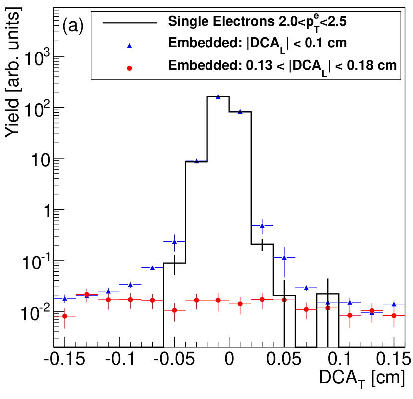
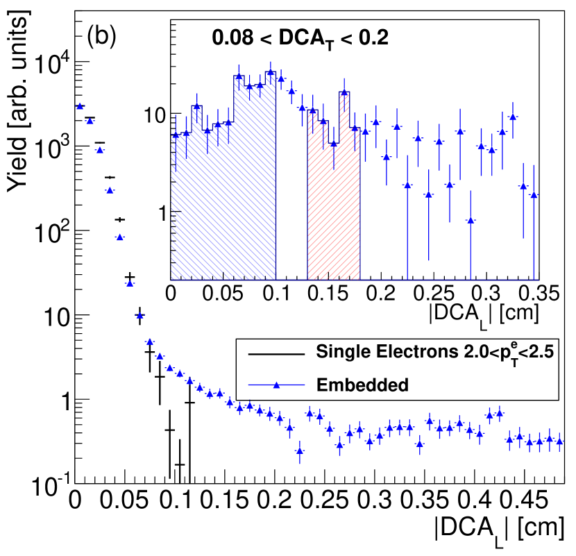
Figure 6: (Color Online) Simulated primary electron (a) $\mathrm{DCA}_{T}$ and (b) $\mathrm{DCA}_{L}$ distribution before and after embedding in real Au$+$Au data.

The reconstructed $\mathrm{DCA}_{T}$ and $\mathrm{DCA}_{L}$ for embedded primary electrons in MB Au$+$Au collisions is shown in Fig. 6. Here the histograms, labeled as “Single Electrons”, show the reconstructed $\mathrm{DCA}_{T}$ and $\mathrm{DCA}_{L}$ distributions of primary electrons before embedding. The $\mathrm{DCA}_{T}$ distribution comprises a narrow Gaussian with no large $\mathrm{DCA}_{T}$ tail and the $\mathrm{DCA}_{L}$ distribution comprises a similar, but slightly broader, Gaussian with no large tail. The blue filled triangles show the $\mathrm{DCA}_{T}$ and $\mathrm{DCA}_{L}$ distributions after embedding. The $\mathrm{DCA}_{T}$ and $\mathrm{DCA}_{L}$ distributions comprise a Gaussian peaked at $\mbox{$\mathrm{DCA}_{T}$}(\mbox{$\mathrm{DCA}_{L}$})\sim 0$ which is consistent with the distribution before embedding. This demonstrates that the DCA resolution of the VTX is not affected by the high multiplicity environment. However, the embedded distributions have broad tails at large $|\mbox{$\mathrm{DCA}_{T}$}|$ and $|\mbox{$\mathrm{DCA}_{L}$}|$.

As shown in Fig. 6(b), tracks with $|\mbox{$\mathrm{DCA}_{L}$}|>0.13$ cm are dominated by random associations, as they are not present in the “Single Electron” sample. We therefore use the $\mathrm{DCA}_{T}$ distribution for tracks with large $|\mbox{$\mathrm{DCA}_{L}$}|$ as an estimate of this random high-multiplicity background. We choose the region $0.13<|\mbox{$\mathrm{DCA}_{L}$}|\ {\rm cm}<0.18$ to represent this background, and restrict our signal to $|\mbox{$\mathrm{DCA}_{L}$}|<0.1$ cm. The $\mathrm{DCA}_{T}$ distribution of tracks with $0.13<|\mbox{$\mathrm{DCA}_{L}$}|\ {\rm cm}<0.18$ must be normalized in order to be used as an estimate of the high-multiplicity background for tracks within $|\mbox{$\mathrm{DCA}_{L}$}|<0.1$ cm. This normalization is determined by matching the integrated yield of embedded primary electrons in each $|\mbox{$\mathrm{DCA}_{L}$}|$ region for $0.08<\mbox{$\mathrm{DCA}_{T}$}\ {\rm cm}<0.2$, as shown in the inlay of Fig. 6(b). The region $0.08<\mbox{$\mathrm{DCA}_{T}$}\ {\rm cm}<0.2$ is dominated by random associations, as shown in Fig. 6(a), and is therefore safe to use for determining the normalization. The normalization of the high-multiplicity background is determined to be $2.89\pm 0.29$. The red filled circles in Fig. 6(a) show the embedded $\mathrm{DCA}_{T}$ distribution with large $\mathrm{DCA}_{L}$ ($0.13<|\mbox{$\mathrm{DCA}_{L}$}|\ {\rm cm}<0.18$). This distribution agrees with the embedded $\mathrm{DCA}_{T}$ distribution (blue filled triangles in Fig. 6) for large $\mathrm{DCA}_{T}$. This demonstrates that the tails for large $\mathrm{DCA}_{T}$ are well normalized by the distribution of electrons with large $\mathrm{DCA}_{L}$. However, there is a small excess in the region $0.05<|\mbox{$\mathrm{DCA}_{T}$}|\ {\rm cm}<0.10$ that is not accounted for by the distribution with large $\mathrm{DCA}_{L}$. We address this excess in the systematic uncertainties, as described in Sec. III.8, where it is found to have only a small effect on the extraction of $b\rightarrow e$ and $c\rightarrow e$.

In each panel of Fig. 5 the high-multiplicity background is shown as a red line. It is determined from the $\mathrm{DCA}_{T}$ distribution of the data within $0.13<|\mbox{$\mathrm{DCA}_{L}$}|\ {\rm cm}<0.18$, as described above. The number of electron tracks in the large $\mathrm{DCA}_{L}$ region is small. We therefore fit the resulting $\mathrm{DCA}_{T}$ data in each $p_{T}$ bin with a smooth function to obtain the shape of the red curves shown in Fig. 5. A second order polynomial is used in the lowest $p_{T}$ bin, where there are enough statistics to constrain it. The higher $p_{T}$ bins are fit with a constant value. All curves are multiplied by the same normalization factor, determined from embedded simulations as described above.

III.5.3 Photonic electrons and conversion veto cut

Photon conversions and Dalitz decays of light neutral mesons ($\pi^{0}$ and $\eta$) are the largest electron background. We refer to this background as photonic electron background as it is produced by external or internal conversion of photons.

The PHENIX Collaboration has previously published the yields of $\pi^{0}$ and $\eta$ mesons in Au$+$Au collisions at $\sqrt{s_{{}_{NN}}}=200$ GeV Adare et al. (2008, 2010b). In addition to the electrons from Dalitz decays of these mesons, the decay photons may convert to an $e^{+}e^{-}$ pair in the detector material in the beam pipe or each layer of the VTX. The PHENIX Collaboration has also published the yields of direct photons in Au$+$Au collisions at $\sqrt{s_{{}_{NN}}}=200$ GeV Afanasiev et al. (2012); Adare et al. (2010a), that can also be a source for conversions.

In principle with these measured yields, combined with simple decay kinematics and a detailed geant3 description of the detector material and reconstruction algorithm, one could fully account for these photonic electron contributions as a function of $\mathrm{DCA}_{T}$ and $p_{T}$. However, systematic uncertainties on the measured yields for the $\pi^{0}$, $\eta$, and direct photons would then dominate the uncertainty of the heavy flavor electron extraction. Therefore, we utilize the VTX detector itself to help reject these contributions in a controlled manner.

We require that at least the first three layers of the VTX have hits associated with the electron track. Conversions in B1 and subsequent layers are rejected by the requirement of a B0 hit, leaving only conversions in B0 and the beam pipe. The requirement of B1 and B2 hits enables us to impose a conversion veto cut, described below, that suppresses conversions from the beam pipe and B0.

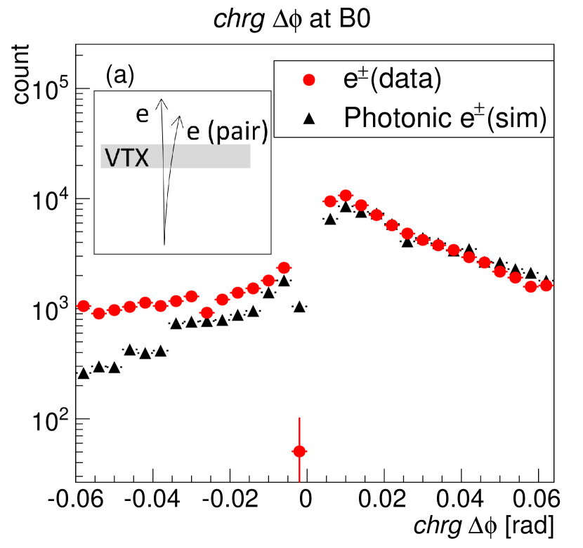
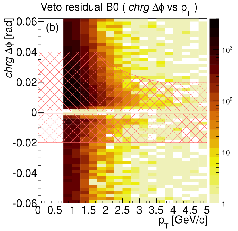
Figure 7: (Color Online) (a) Distribution of correlated hits in B0 near electron tracks for $1<p_{T}<2$ GeV/$c$. The red (circle) points are from Au$+$Au data and the black (triangle) points are from Monte Carlo simulation. The insert in (a) illustrates the electron pairs from Dalitz decays. (b) The window of the conversion veto cut for B0 layer (hatched) and the hit distribution near electron track in 2D space of $chrg\ \Delta\phi$ vs $p_{T}$ of electrons in Au$+$Au collisions. (See the text for details).

The conversion veto cut rejects tracks with another VTX hit within a certain window in $\Delta\phi$ and $\Delta z$ around hits associated with a VTX-associated track. Photons that convert to an $e^{+}e^{-}$ pair in the beam pipe will leave two nearby hits in the first layer (B0) and/or subsequent layers of the VTX, and thus be rejected by the conversion veto cut. Similarly, conversions in B0 will result in two nearby hits in the second layer (B1) and/or subsequent outer layers. The same is true for $e^{+}e^{-}$ from a Dalitz decay, though with a larger separation due to a larger opening angle of the pair.

Figure 7(a) shows distribution of $chrg\ \Delta\phi$ of hits in B0 relative to the electron track, where $chrg$ is the charge of the track. The red (circle) histogram shows the data in MB Au$+$Au collisions. If the track at the origin is not an electron, we have a flat distribution due to random hits in the detector. These random hits have been subtracted in Fig. 7(a). The transverse momentum of the electron track is in the interval $1<p_{T}\ \mbox{GeV/$c$}<2$.

As mentioned above, these correlated hits around electron tracks are caused by the partner $e^{+}$ or $e^{-}$ of Dalitz decays or photon conversions. The left-right asymmetry of the distribution is caused by the fact that the partner $e^{\pm}$ track is separated from the electron track by the magnetic field and the direction of the separation is determined by the charge of the electron track. In the distribution of $chrg\ \Delta\phi$, the partner track is bent towards the positive direction.

The black (triangle) histogram in Fig. 7(a) shows the distribution from Monte Carlo simulations. In the simulation, the response of the PHENIX detector to single $\pi^{0}$s is modeled by geant3, and the resulting hits in the VTX and the central arms are then reconstructed by the same reconstruction code as the data. The correlated hits in the simulation are caused by the Dalitz decay of $\pi^{0}$ and photon conversion in the material of the beam pipe and the VTX itself. The simulation reproduces the data well for $chrg\ \Delta\phi>0$. There is a difference between the data and the simulation for $chrg\ \Delta\phi<0$. This is caused by a subtle interplay between the conversions and high multiplicity effects. The difference disappears for peripheral collisions. Similar correlated hits are observed in B1 to B3 layers in the data and they are also well explained by the simulation.

We define a “window” of the conversion veto cut around an electron track in each layer B0 to B3 and require that there is no hit other than the hit associated with the electron track in the window. Since a photonic electron (Dalitz and conversion) tends to have a correlated hit in the window, as one can see in Fig. 7, this conversion veto cut rejects photonic background. A larger window size can reject photonic background more effectively, but this can also reduce the efficiency for the heavy flavor electron signal due to random hits in the window. The window for the conversion veto cut is a compromise in terms of the rejection factor on photonic backgrounds and efficiency for heavy flavor electrons. We optimized the size of the window of the conversion veto cut based on a full geant3 simulation.

The red hatched area shown in Fig. 7(b) shows the window of the conversion veto cut in layer B0. The window size is asymmetric since correlated hits are mainly in the positive side of $chrg\ \Delta\phi$. The window size is reduced for higher electron $p_{T}$ since the distribution of correlated hits becomes narrower for higher $p_{T}$. The windows for B1-B3 are similarly determined based on geant3 simulation.

Figure 8 shows the survival fraction of the conversion veto cut for electrons from photon conversions and Dalitz decays as a function of electron $p_{T}$ from a full geant3 simulation of the detector with hits run through the reconstruction software. The survival probability for conversions is less than 30% at $\mbox{$p_{T}$}=1$ GeV/$c$ and decreases further at higher $p_{T}$. The survival probability for Dalitz decays is higher since a Dalitz decay partner is more likely to fall outside of the window of the conversion veto cut due to the larger opening angle. Also shown in Fig. 8 is the survival fraction of electrons from heavy flavor decays which pass the conversion veto cut ($S_{\rm HF}$). As expected, their efficiency for passing the conversion veto cut is quite high and $p_{T}$ independent.

The efficiencies shown in Fig. 8 are calculated without the Au$+$Au high-multiplicity that may randomly provide a hit satisfying the conversion veto cut. Since these are random coincidences, they are a common reduction for all sources including the desired signal — heavy flavor electrons. This common reduction factor, $\delta_{random}$, is measured from the reduction of the hadron track yield by the conversion veto cut to be $\simeq$ 35% at $\mbox{$p_{T}$}=1$ GeV/$c$ to $\simeq$ 25% at $\mbox{$p_{T}$}=5$ GeV/$c$ for MB Au$+$Au collisions. Note that when we determine the $\mathrm{DCA}_{T}$ distribution of the various background components using a full geant3 simulation we apply the same conversion veto cuts.

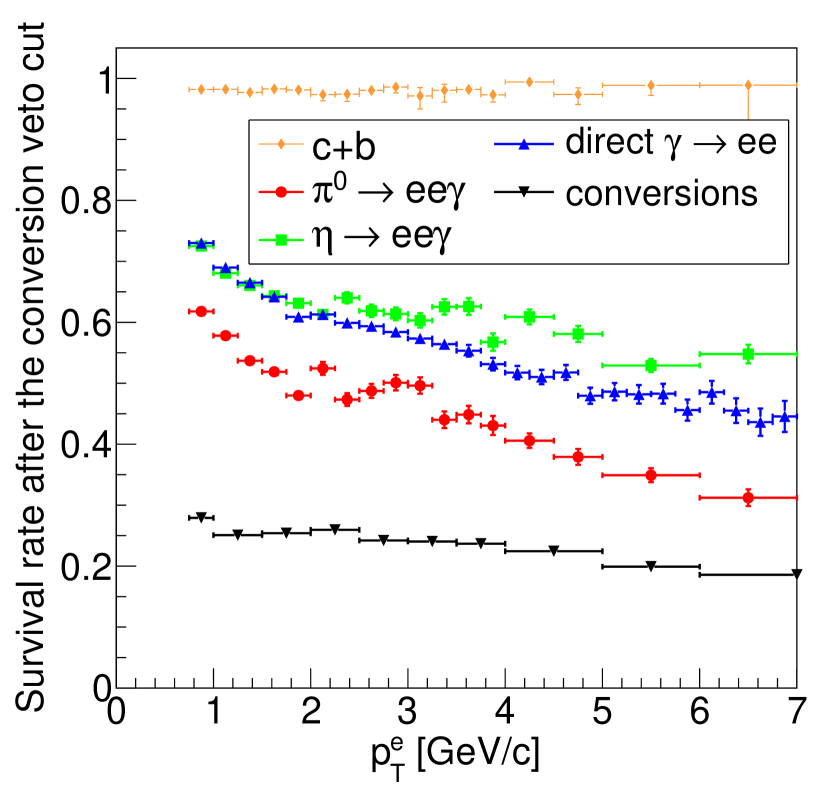
Figure 8: (Color Online) The survival rate as a function of electron $p_{T}$ ($p_{T}^{e}$) for electrons from photon conversion (black), Dalitz decay of $\pi^{0}$ (red), $\eta$ (green), electrons from direct photon (blue) and heavy flavor decay electrons (dark orange).

The $\mathrm{DCA}_{T}$ distributions from photonic background processes that survive the conversion veto cut are shown in Fig. 5. The means of the $\mathrm{DCA}_{T}$ distributions from Dalitz decays and conversions are shifted to negative $\mathrm{DCA}_{T}$ values due to the mis-reconstruction of the momentum caused by the assumption that the tracks originate at the primary vertex, as explained in the next paragraph. The shift is largest at the lowest $p_{T}$ bin and decreases with increasing $p_{T}$.

For Dalitz electrons, the shift is due to the energy loss via induced radiation (bremsstrahlung). The total radiation length of the VTX is approximately 13% as shown in Table 1. Thus a Dalitz electron coming from the primary vertex loses approximately $1-e^{-0.13}\approx{12}$% of its energy on average when it passes through the VTX. The momentum measured by the DC is close to the one after the energy loss due to the reconstruction algorithm. Since the momentum determined by the DC is used when projecting inward from the hit in B0 to the primary vertex and in calculation of $\mathrm{DCA}_{T}$, this results in a slight shift in the $\mathrm{DCA}_{T}$ distribution. This effect is fully accounted for in the $\mathrm{DCA}_{T}$ template of Dalitz electrons since it is generated through the full geant3 and reconstruction simulation.

In the case of conversions, the effect is even larger, as one can clearly see in Fig. 5. While a photon goes straight from the primary vertex to the beam pipe or B0 layer where it converts, $\mathrm{DCA}_{T}$ is calculated assuming that the electron track is bent by the magnetic field. Thus the $\mathrm{DCA}_{T}$ distribution is shifted by the difference of the actual straight line trajectory and the calculated bent trajectory. Again, this is fully accounted for with the full geant3 simulation. The effect is verified by selecting conversion electrons with a reversed conversion veto cut.

III.5.4 $K_{e3}$

The background from $K_{e3}$ decays ($K^{0}_{S}$, $K^{\pm}$ $\rightarrow e\nu\pi$) contributes electrons over a broad range of $\mathrm{DCA}_{T}$ due to the long lifetime of the kaons. Both contributions are determined using pythia and a full geant3 simulation, taking into account the exact track reconstruction, electron identification cuts, and conversion veto cut. The resulting $\mathrm{DCA}_{T}$ distribution for these kaon decays is shown in Fig. 5. As expected, though the overall yield is small, this contributes at large $\mathrm{DCA}_{T}$ in the lower $p_{T}$ bins and is negligible at higher $p_{T}$.

III.5.5 Quarkonia

Quarkonia ($J/\psi$ and $\Upsilon$) decay into electron pairs. Due to the short lifetime, these decays contribute to electrons emanating from the primary vertex. The $J/\psi$ yields in Au$+$Au collisions at $\sqrt{s_{{}_{NN}}}=200$ GeV have been measured by the PHENIX Collaboration Adare et al. (2007b). The detailed modeling of these contributions out to high $p_{T}$ is detailed in Ref. Adare et al. (2011). While these measurements include a small fraction of $B\rightarrow J/\psi$ decays, all $J/\psi$’s are considered prompt when modeling the $\mathrm{DCA}_{T}$ distribution. The $J/\psi$ contribution is shown in Fig. 5, and is quite small and peaked about $\mathrm{DCA}_{T}$ = 0 as expected. Thus, the systematic uncertainty from the quarkonium yields in Au$+$Au collisions is negligible in all electron $p_{T}$ bins.

III.6 Normalization of electron background components

If the detector performance were stable, we could convert the $\mathrm{DCA}_{T}$ distributions from counts into absolutely normalized yields. Then one could straightforwardly subtract the similarly absolutely normalized background contributions described above—with the normalization constrained by the previously published PHENIX yields for $\pi^{0}$, $\eta$, etc. However, due to detector instability during the 2011 run, such absolute normalization of background contributions can have a large systematic uncertainty. Thus we bootstrap the relative normalization of these background contributions utilizing our published Au$+$Au results Adare et al. (2011) from data taken in 2004.

The idea of the method is the following. PHENIX measured the invariant yield of open heavy flavor decay electrons from the 2004 dataset. In this 2004 analysis we first measured inclusive electrons (i.e. the sum of background electrons and heavy flavor electrons). We then determined and subtracted the background electron components from the inclusive electron yields to obtain the heavy flavor contribution. Thus the ratio of the background components to the heavy flavor contribution were determined and published in Adare et al. (2011). We use these ratios to determine the normalization of background components in the 2011 data, as described in the next paragraph. Some backgrounds have the same ratio to signal regardless of the year the data was collected, while others will differ due to the additional detector material added by the VTX.

The invariant yield in Au$+$Au collisions at $\sqrt{s_{{}_{NN}}}=200$ GeV of heavy flavor electrons and background electrons from Dalitz decays is a physical observable independent of the year the data was taken. Thus we can use the ratio of heavy flavor/Dalitz that is determined in the 2004 analysis in the 2011 data. On the other hand, the invariant yield of conversion electrons depends on the detector material present and is thus different in the 2011 data taking period with the VTX installed compared with the 2004 data. We account for this difference by calculating the fraction of nonphotonic electrons in the 2011 data. A detailed description of the normalization procedure is given in Appendix APPENDIX: Detailed Normalization of electron background components.

With this bootstrapped normalization completed, the correctly normalized background components are shown for all five $p_{T}$ bins vs $\mathrm{DCA}_{T}$ in Fig. 5. Note that the normalization of mis-identified hadron and random background is determined from the data as explained in sections III.5.1 and  III.5.2, respectively. The electron yield beyond the sum of these background components is from the combination of charm and bottom heavy flavor electrons.

III.7 Unfolding

III.7.1 Introduction

With the $\mathrm{DCA}_{T}$ distributions as a function of electron $p_{T}$ and the various background components in hand, we proceed to extract the remaining charm and bottom components. If one knew the shape of the parent charm and bottom hadron $p_{T}$ and rapidity distributions, one could calculate in advance the $\mathrm{DCA}_{T}$ shape for electrons from each heavy flavor via a model of the decay kinematics. Since the decay lengths of charm and bottom hadrons are significantly different, they will yield different $\mathrm{DCA}_{T}$ distributions. In this case, one could simultaneously fit the $\mathrm{DCA}_{T}$ distribution for each $p_{T}$ bin with all background components fixed across $p_{T}$ bins, and extract the one free parameter: the ratio of charm to bottom contributions. However, the $p_{T}$ distribution of charm hadrons is known to be significantly modified in Au$+$Au collisions — see for example Ref. Adamczyk et al. (2014). For bottom hadrons this is also likely to be the case. Therefore one does not know a priori the heavy flavor $\mathrm{DCA}_{T}$ distribution since it depends on the parent $p_{T}$ distribution.

Since the $\mathrm{DCA}_{T}$ distributions for all electron $p_{T}$ result from the same parent charm and bottom hadron $p_{T}$ spectrum, one can perform a simultaneous fit to all the electron $p_{T}$ and $\mathrm{DCA}_{T}$ data in order to find the most likely heavy flavor parent hadron $p_{T}$ distributions. The estimation of a set of most likely model parameters using a simultaneous fit to data is often referred to as unfolding. Statistical inference techniques are often employed to solve such problems; see for example the extraction of reconstructed jet cross sections Cowan (2002).

The $\mathrm{DCA}_{T}$ distributions are in counts and have not been corrected for the $p_{T}$-dependent reconstruction efficiency in Au$+$Au collisions, and therefore hold no yield information. To further constrain the extraction of the charm and bottom components, we include the total heavy flavor electron invariant yield as measured by PHENIX Adare et al. (2011) in Au$+$Au collisions at $\sqrt{s_{{}_{NN}}}=200$ GeV. This measurement is more accurate than currently available with the 2011 data set, where the VTX acceptance changes with time.

The unfolding procedure, using a particular sampling method (described in Section III.7.2), chooses a set of trial charm and bottom parent hadron yields. The trial set of yields is multiplied by a decay matrix (described in Section III.7.4), which encodes the probability for a hadron in a given $p_{T}$ interval to decay to an electron at midrapidity as a function of electron $p_{T}$ and $\mathrm{DCA}_{T}$. The resulting distributions of electron $p_{T}$ and $\mathrm{DCA}_{T}$ are compared with the measured data using a likelihood function (described in Section III.7.3). In order to dampen discontinuities and oscillatory behavior, a penalty upon the likelihood (described in Section III.7.5) is added to enforce smoothness in the resulting hadron $p_{T}$ distributions.

III.7.2 Unfolding method

Here we apply Bayesian inference techniques to the unfolding problem. A detailed pedagogical introduction to these techniques is given in Ref. Choudalakis . Techniques involving maximum likelihood estimation or maximum a posteriori estimation, often used in frequentist statistics, can at best compute only a point estimate and confidence interval associated with individual model parameters. In contrast, Bayesian unfolding techniques have the important advantage of providing a joint probability density over the full set of model parameters. In this analysis, the vector of model parameters, $\boldsymbol{\theta}$, is the vector of parent charm and bottom hadron yields binned in $p_{T}$.

Given a vector of measured data, $\mathbf{x}$, and our vector of model parameters, $\boldsymbol{\theta}$, we use Bayes’ theorem

$$p(\boldsymbol{\theta}|\mathbf{x})=\frac{P(\mathbf{x}|\boldsymbol{\theta})\pi(\boldsymbol{\theta})}{P(\mathbf{x})},$$ (2)

to compute the posterior probability density $p(\boldsymbol{\theta}|\mathbf{x})$ from the likelihood $P(\mathbf{x}|\boldsymbol{\theta})$ and prior information $\pi(\boldsymbol{\theta})$. The function $P(\mathbf{x}|\boldsymbol{\theta})$, quantifies the likelihood of observing the data given a vector of model parameters. In frequentist statistics, the $P(\mathbf{x}|\boldsymbol{\theta})$ is often used alone to determine the best set of model parameters. Bayesian inference, on the other hand, allows for the inclusion of the analyzer’s a priori knowledge about the model parameters, as encoded in $\pi(\boldsymbol{\theta})$. The implementation of $\pi(\boldsymbol{\theta})$ used in this analysis is discussed in Sec. III.7.5. The denominator $P(\mathbf{x})$ serves as an overall normalization of the combined likelihood $P(\mathbf{x}|\boldsymbol{\theta})\pi(\boldsymbol{\theta})$ such that $p(\boldsymbol{\theta}|\mathbf{x})$ can be interpreted as a probability density. In this analysis, $p(\boldsymbol{\theta}|\mathbf{x})$ gives the probability for a set of charm and bottom hadron yields,

$$\boldsymbol{\theta}=(\boldsymbol{\theta}_{c};\boldsymbol{\theta}_{b}),$$ (3)

given the values of the measured electron data points $\mathbf{x}$. Since we are only interested in the parameters which maximize $p(\boldsymbol{\theta}|\mathbf{x})$, we can dispense with the calculation of $P(\mathbf{x})$, as it serves only as an overall normalization.

Here $\boldsymbol{\theta}$ comprises 17 bins of both charm and bottom hadron $p_{T}$, yielding a 34-dimensional space which must be sampled from in order to evaluate $p(\boldsymbol{\theta}|\mathbf{x})$. To accomplish this we employ a Markov Chain Monte Carlo (MCMC) algorithm to draw samples of $\boldsymbol{\theta}$ in proportion to $p(\boldsymbol{\theta}|\mathbf{x})$. This makes accurate sampling of multidimensional distributions far more efficient than uniform sampling. In implementation, it is in fact the right hand side of Eq. 2 that is sampled. The MCMC variant used here is an affine-invariant ensemble sampler described in Ref. Goodman, J. and Weare, J (2010) and implemented as described in Ref. Foreman-Mackey et al. (2013). It is well suited to distributions that are highly anisotropic such as spectra which often vary over many orders of magnitude.

III.7.3 Modeling the likelihood function

This analysis is based on 21 data points of total heavy flavor electron invariant yield, $\mathbf{Y}^{\rm data}$, in the range 1.0–9.0 GeV/$c$ from the 2004 data set Adare et al. (2011), and five electron $\mathrm{DCA}_{T}$ distributions $\mathbf{D}_{j}^{\rm data}$, where $j$ indexes each electron $p_{T}$ interval within the range 1.5–5.0 GeV/$c$ from the 2011 data set. Therefore,

$$\mathbf{x}=(\mathbf{Y}^{\rm data},\mathbf{D}_{0}^{\rm data},\mathbf{D}_{1}^{\rm data},\mathbf{D}_{2}^{\rm data},\mathbf{D}_{3}^{\rm data},\mathbf{D}_{4}^{\rm data})$$ (4)

in Eq. 2.

Our ultimate goal is to accurately approximate the posterior distribution over the parent hadron invariant yields $\boldsymbol{\theta}$ by sampling from it. For each trial set of hadron yields, the prediction in electron $p_{T}$, $\mathbf{Y}(\boldsymbol{\theta})$, and $\mathrm{DCA}_{T}$, $\mathbf{D}_{j}(\boldsymbol{\theta})$, is calculated by

$$\mathbf{Y}(\boldsymbol{\theta}) =\mathbf{M}^{\mathbf{(Y)}}\boldsymbol{\theta}_{c}+\mathbf{M}^{\mathbf{(Y)}}\boldsymbol{\theta}_{b}$$ (5)

$$\mathbf{D}_{j}(\boldsymbol{\theta}) =\mathbf{M}_{j}^{\mathbf{(D)}}\boldsymbol{\theta}_{c}+\mathbf{M}_{j}^{\mathbf{(D)}}\boldsymbol{\theta}_{b},$$ (6)

where $\mathbf{M}^{\mathbf{(Y)}}$ and $\mathbf{M}_{j}^{\mathbf{(D)}}$ are decay matrices discussed in Section III.7.4. We then evaluate the likelihood between the prediction and each measurement in the data sets $\mathbf{Y}^{\rm data}$ and $\{\mathbf{D}_{j}^{\rm data}\}_{j=0}^{4}$. As is customary, the logarithm of the likelihood function is used in practice. The combined (log) likelihood for the data is explicitly

$$\small\ln P(\mathbf{x}|\boldsymbol{\theta})=\ln P(\mathbf{Y}^{\rm data}|\mathbf{Y}(\boldsymbol{\theta}))+\sum_{j=0}^{4}\ln P(\mathbf{D}_{j}^{\rm data}|\mathbf{D}_{j}(\boldsymbol{\theta})).$$ (7)

The $\mathbf{Y}^{\rm data}$ dataset is assigned statistical uncertainties that are assumed to be normally distributed and uncorrelated. Thus, the likelihood $\ln P(\mathbf{Y}^{\rm data}|\mathbf{Y}(\boldsymbol{\theta}))$ is modeled as a multivariate Gaussian with diagonal covariance. The systematic uncertainties on the $\mathbf{Y}^{\rm data}$ dataset and their effect on the unfolding result are discussed in Sec. III.8.

The $\mathrm{DCA}_{T}$ data sets, in contrast, each comprise a histogrammed distribution of integer-valued entries, and the likelihood $\ln P(\mathbf{D}_{j}^{\rm data}|\mathbf{D}_{j}(\boldsymbol{\theta}))$ is thus more appropriately described by a multivariate Poisson distribution. However, the likelihood calculation for the $\mathrm{DCA}_{T}$ data sets requires three additional considerations. First, there are significant background contributions from a variety of sources, as discussed in Section III.5. Secondly, detector acceptance and efficiency effects are not explicitly accounted for in the $\mathrm{DCA}_{T}$ distributions. This implies that the total measured yield of signal electrons in each $\mathrm{DCA}_{T}$ histogram is below what was actually produced, and consequently the measured $\mathbf{D}_{j}^{\rm data}$ distributions do not match the predictions in normalization. Lastly, because of the high number of counts in the region near $\mathrm{DCA}_{T}$ $=0$, this region will dominate the likelihood and be very sensitive to systematic uncertainties in the $\mathrm{DCA}_{T}$ shape there, even though the main source of discrimination between charm and bottom electrons is at larger $\mathrm{DCA}_{T}$.

To deal with the first issue, the relatively normalized background described in Sec. III.5 is added to each prediction of the $\mathrm{DCA}_{T}$ distribution for summed electrons from charm and bottom hadrons so that the shape and relative normalization of the background component of the measurement is accounted for.

To handle the second, each prediction plus the background is scaled to exactly match the normalization of $\mathbf{D}_{j}^{\rm data}$. In this way, only the shape of the prediction is a constraining factor.

To deal with the third, a 5% uncertainty is added in quadrature to the statistical uncertainty when the number of counts in a given $\mathrm{DCA}_{T}$ bin is greater than a reasonable threshold (which we set at 100 counts). This accounts for the systematic uncertainty in the detailed $\mathrm{DCA}_{T}$ shape by effectively de-weighting the importance of the region $\mbox{$\mathrm{DCA}_{T}$}\approx$0 while maintaining the overall electron yield normalization (as opposed to removing the data entirely). This additional uncertainty also necessitates changing the modeling of $\ln P(\mathbf{D}_{j}^{\rm data}|\mathbf{D}_{j}(\boldsymbol{\theta}))$ from a Poisson to a Gaussian distribution. We have checked that varying both the additional uncertainty and the threshold at which it is added has little effect on the results.

III.7.4 Decay model and matrix normalization

The pythia-6 Sjostrand et al. generator with heavy flavor production process included, via the parameter MSEL=4(5), is used to generate parent charm (bottom) hadrons and their decays to electrons. Electrons within $|\eta|<0.35$ decayed from the ground state charm hadrons ($D^{\pm}$, $D^{0}$, $D_{s}$, and $\Lambda_{c}$) or bottom hadrons ($B^{\pm}$, $B^{0}$, $B_{s}$, and $\Lambda_{b}$) are used to create a decay matrix between hadron $p_{T}$ ($p_{T}^{h}$, representing charm hadron $p_{T}$, $p_{T}^{c}$, or bottom hadron $p_{T}$, $p_{T}^{b}$) and electron $p_{T}$ ($p_{T}^{e}$) and $\mathrm{DCA}_{T}$. Here we treat the feed down decay $B\rightarrow D\rightarrow e$ as a bottom hadron decay and exclude it from charm hadron decays.

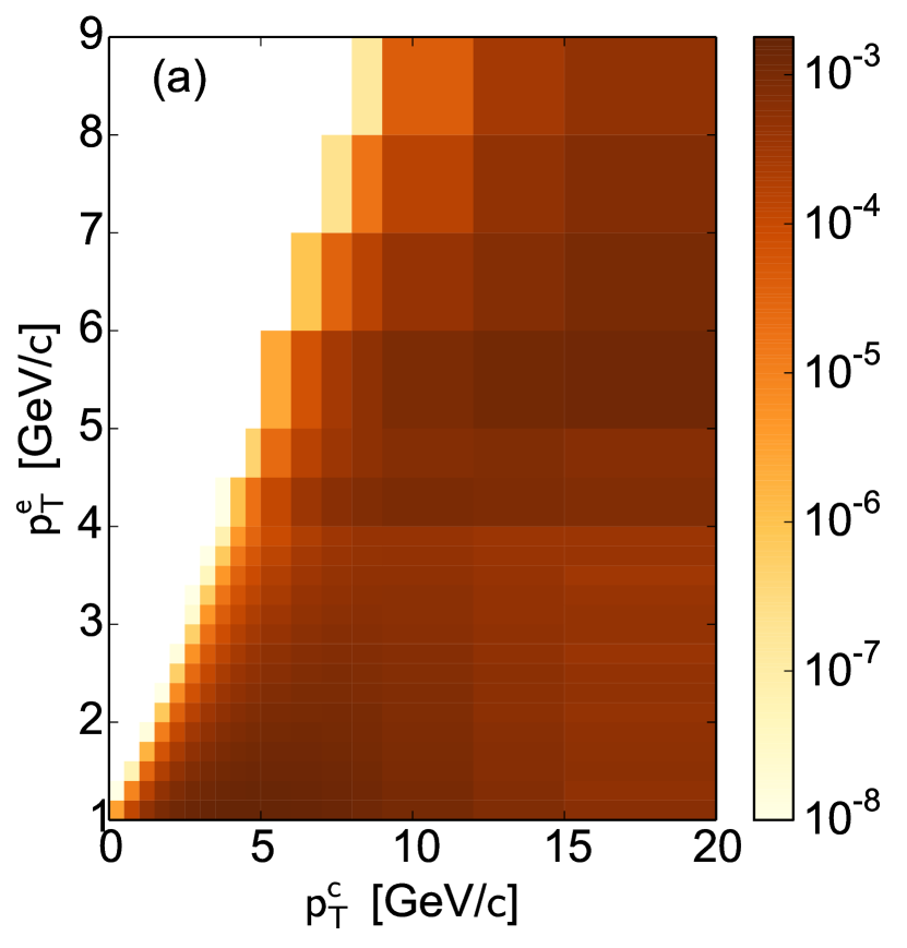
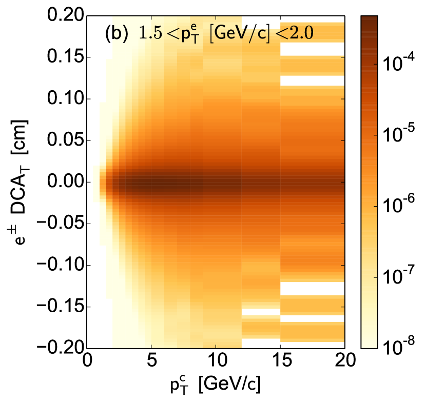
Figure 9: (Color Online) (a) The decay matrix, $\mathbf{M}^{\mathbf{(Y)}}$, encoding the probability for charmed hadrons decaying to electrons within $|\eta|<0.35$ as a function of both electron $p_{T}$ ($p_{T}^{e}$) and charm hadron $p_{T}$ ($p_{T}^{c}$). (b) An example decay matrix, $\mathbf{M}_{j}^{\mathbf{(D)}}$, encoding the probability for charmed hadrons decaying to electrons within $|\eta|<0.35$ and $1.5<\mbox{$p_{T}^{e}$}\ [{\rm~{}GeV}/c]<2.0$ as a function of both electron $\mathrm{DCA}_{T}$ and charm hadron $p_{T}$ ($p_{T}^{c}$). In both cases the color intensity represents the probability of decay in the given bin.

The probability for a charm or bottom hadron at a given $p_{T}^{h}$ to decay to an electron at a given $p_{T}^{e}$ and $\mathrm{DCA}_{T}$ is encoded in the multidimensional matrices $\mathbf{M}^{\mathbf{(Y)}}$ and $\mathbf{M}_{j}^{\mathbf{(D)}}$. An example decay matrix for charmed hadrons is shown in Fig. 9. Note that the 17 bins in $p_{T}^{c}$ correspond to the same bins shown along the $x$-axis in Fig. 15, and that the binning in $p_{T}^{e}$ and $\mathrm{DCA}_{T}$ seen in Fig. 9 is the same as that shown in Fig. 12 and Fig. 13 respectively. Furthermore, note that the marginal probabilities do not integrate to unity in these matrices. This is because the decay probabilities are normalized to the number of hadrons that are generated at all momenta, in all directions, and over all decay channels. The probability distribution for a hadron integrated over all rapidities and decay channels within a given $p_{T}^{h}$ range to decay to an electron at $|y|<0.35$ with a given $p_{T}^{e}$ (integrated over $\mathrm{DCA}_{T}$) is shown in Fig. 10 for an example set of $p_{T}^{h}$ bins.

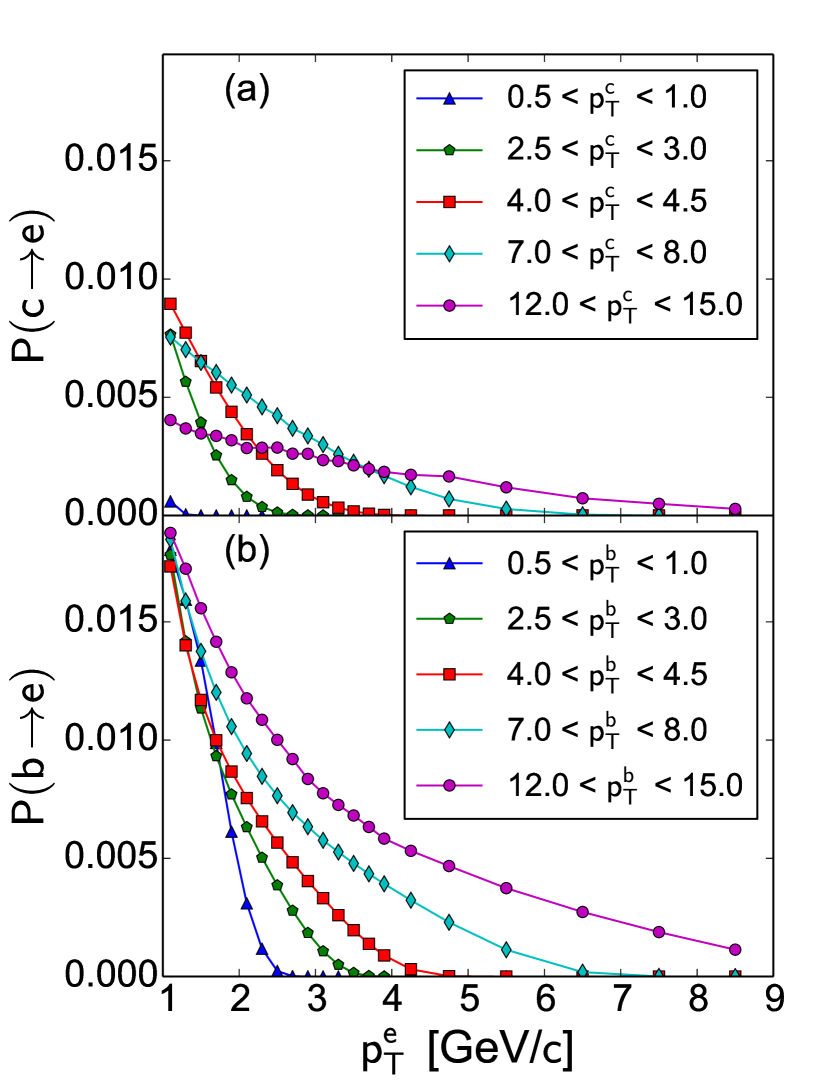
Figure 10: (Color Online) The probability for (a) charm and (b) bottom hadrons in a given range of hadron $p_{T}$ ($p_{T}^{c}$ and $p_{T}^{b}$ for charm and bottom hadrons respectively) to decay to electrons at midrapidity as a function of electron $p_{T}$ ($p_{T}^{e}$).

In principle, this decay matrix introduces a model dependence to the result. In the creation of the decay matrix we are integrating over all hadron rapidities as well as combining a number of hadron species and their decay kinematics to electrons. This involves two assumptions. The first is that the rapidity distributions of the hadrons are unmodified. BRAHMS found that the pion and proton $R_{AA}$ did not depend strongly on rapidity up to $y\approx 3$ Staszel (2006), justifying the assumption. This assumption will further lead us to quote charm and bottom hadron yields as a function of $p_{T}$ integrated over all rapidity. The second assumption is that all ground state charm hadrons experience the same modification as a function of $p_{T}^{c}$. While different than the charm suppression, all bottom hadrons are assumed to experience the same modification.

An enhancement in the baryon to meson production ratios in both nonstrange and strange hadrons has been measured at RHIC Abelev et al. (2006), which may carry over into the heavy quark sector, invalidating the second assumption. While there are some models Martinez-Garcia et al. (2008) that attempt to incorporate this anomalous enhancement into the charm hadrons to help explain the measured heavy flavor electron $R_{AA}$, there are few measurements to help constrain this proposed enhancement. Following Ref. Sorensen and Dong (2006), we have tested the effect of this assumption by applying the observed baryon/meson enhancement to both the $\Lambda_{c}/D$ and $\Lambda_{b}/B$ ratios. As in Ref. Sorensen and Dong (2006), we assume that the modification asymptotically approaches 1 for hadron $\mbox{$p_{T}$}>8$ GeV/$c$. We find that including the enhancement gives a lower charm hadron yield at high-$p_{T}$ and a larger bottom hadron yield at high-$p_{T}$, but the modifications are within the systematic uncertainties discussed in Sec. III.8 and shown in Fig. 15. We also find a larger bottom electron fraction, which is again within the systematic uncertainties shown in Fig. 17. While we have not used other particle generators to create alternate decay matrices, we find that the $D^{0}$ and $D^{\pm}$ meson $p_{T}$ and rapidity distributions from pythia are similar to those given by Fixed Order + Next-to-Leading Log (fonll) calculations Cacciari et al. (2005). We have not included any systematic uncertainty due to this model dependence in the final result.

III.7.5 Regularization/prior

To penalize discontinuities in the unfolded distributions of charm and bottom hadrons, we include a regularization term to the right hand side of equation 7. In this analysis we included a squared-exponential function

$$\ln\pi(\boldsymbol{\theta})=-\alpha^{2}\left(|\mathbf{L}\mathbf{R}_{c}|^{2}+|\mathbf{L}\mathbf{R}_{b}|^{2}\right)$$ (8)

where $\mathbf{R}_{c}$ and $\mathbf{R}_{b}$ are ratios of the charm and bottom components of the parent hadron $p_{T}$ vector to the corresponding 17 components of the prior, $\boldsymbol{\theta}_{{\rm prior}}$, and $\mathbf{L}$ is a 17-by-17 second-order finite-difference matrix of the form

$$\mathbf{L}=\frac{17}{2}\begin{pmatrix}-1&1&&&&&&\\ 1&-2&1&&&&&\\ &1&-2&1&&&&\\ &&\ddots&\ddots&\ddots&&&&\\ &&&\ddots&\ddots&\ddots&&&\\ &&&&1&-2&1&\\ &&&&&1&-2&1\\ &&&&&&1&-1\end{pmatrix}.$$ (9)

Thus the addition of this term encodes the assumption that departures from $\boldsymbol{\theta}_{{\rm prior}}$ should be smooth by penalizing total curvature as measured by the second derivative.

Here, $\alpha$ is a regularization parameter set to $\alpha=1.0$ in this analysis. We determine $\alpha$ by repeating the unfolding procedure, scanning over $\alpha$ and choosing the value of $\alpha$ which maximizes the resulting sum of Eq. 7 and $-\left(|\mathbf{L}\mathbf{R}_{c}|^{2}+|\mathbf{L}\mathbf{R}_{b}|^{2}\right)$ (Eq. 8 dropping $\alpha^{2}$). In this way we can directly compare log likelihood values for unfolding results with different $\alpha$ values. We include variations on $\alpha$ in the systematic uncertainty as described in Section III.8.

We set $\boldsymbol{\theta}_{{\rm prior}}$ to pythia charm and bottom hadron $p_{T}$ distributions scaled by a modified blast wave calculation Adare et al. (2014b) which asymptotically approaches $R_{AA}$ values of 0.2(0.3) for $D$($B$) mesons at high-$p_{T}$. We have tested the sensitivity of the result to $\boldsymbol{\theta}_{{\rm prior}}$ by alternatively using unmodified pythia charm and bottom hadron $p_{T}$ distributions. We find that the result is sensitive to the choice of $\boldsymbol{\theta}_{\rm prior}$ dominantly in the lowest charm hadron $p_{T}$ bins, where there is minimal constraint from the data. We have included this sensitivity in the systematic uncertainty as discussed in Section III.8.

III.7.6 Parent charm and bottom hadron yield and their statistical uncertainty

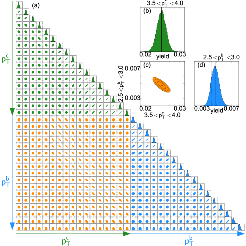
Figure 11: (Color Online) The joint probability distributions for the vector of hadron yields, $\boldsymbol{\theta}$, showing the 2-D correlations between parameters. The diagonal plots show the marginalized probability distributions for each hadron $p_{T}$ bin (i.e. the 1-dimensional projection over all other parameters). Along the Y-axis the plots are organized from top to bottom as the 17 charm hadron $p_{T}$ ($p_{T}^{c}$) bins from low to high $p_{T}^{c}$ followed by the 17 bottom hadron $p_{T}$ ($p_{T}^{b}$) bins from low to high $p_{T}^{b}$. The X-axis is organized similarly from left to right. The $p_{T}^{c}$ and $p_{T}^{b}$ binning follows that shown in Fig. 15. The region of green plots (top left quadrant) shows the charm hadron yields and the correlations between charm hadron yields. The region of blue plots (bottom right quadrant) shows the bottom hadron yields and correlations between bottom hadron yields. The region of orange plots (bottom left quadrant) shows the correlations between charm and bottom hadron yields. Sub-panels (b)-(d) show a set of example distributions. (b) The 1-D probability distribution of charm hadron yield in $3.5<\mbox{$p_{T}^{c}$}\ \mbox{GeV/$c$}<4.0$. (d) The 1-D probability distribution of bottom hadron yield in $2.5<\mbox{$p_{T}^{b}$}\ \mbox{GeV/$c$}<3.0$. (c) The correlation between (b) and (d).

The outcome of the sampling process is a distribution of $\boldsymbol{\theta}$ vectors, which is 34-dimensional in this case. In principle, the distribution of $\boldsymbol{\theta}$ vectors contains the full probability, including correlations between the different parameters. The 2-D correlations are shown in Fig. 11. While it is difficult to distinguish fine details in the 34$\times$34-dimensional grid of correlation plots, we can see a few gross features. A circular contour in the 2-D panels represents no correlation between the corresponding hadron $p_{T}$ bins. An oval shape with a positive slope indicates a positive correlation between corresponding bins, and an oval shape with a negative slope represents an anti-correlation between corresponding bins. A large positive correlation is seen for adjacent bins for high-$p_{T}$ charm hadrons and low-$p_{T}$ bottom hadrons. This is a consequence of the regularization, which requires a smooth $p_{T}$ distribution, and is stronger at the higher and lower $p_{T}$ regions where there is less constraint from the data. We also see that, while there is little correlation between the majority of nonadjacent $p_{T}$ bins, there does seem to be a region of negative correlation between the mid to high $p_{T}$ charm hadrons and the low to mid $p_{T}$ bottom hadrons. Charm and bottom hadrons in these regions contribute decay electrons in the same $p_{T}$ region, and appear to compensate for each other to some extent. An example of this is shown between $3.5<\mbox{$p_{T}^{c}$}\ \mbox{GeV/$c$}<4.0$ and $2.5<\mbox{$p_{T}^{b}$}\ \mbox{GeV/$c$}<3.0$ in Fig. 11(b)-(d).

To summarize $p(\boldsymbol{\theta}|\mathbf{x})$, we take the mean of the marginalized posterior distributions (the diagonal plots in Fig. 11) for each hadron $p_{T}$ bin as the most likely values, and the 16^th and 84^th quantiles to represent the $\pm 1\sigma$ uncertainty in those values due to the statistical uncertainty in the data modified by the regularization constraint.

III.7.7 Re-folded comparisons to data

The vector of most likely hadron yields, with uncertainties, can be multiplied by the decay matrix to check the consistency of the result with the measured data (here referred to as re-folding). Figure 12 shows the measured heavy flavor electron invariant yield in Au$+$Au collisions Adare et al. (2011) compared with the re-folded electron spectra from charm and bottom hadrons. We find good agreement between the measured data and the electron spectrum from the re-folded charm and bottom hadron yields. Figure 13 shows the comparison in electron $\mathrm{DCA}_{T}$ space for each bin in electron $p_{T}$. Shown in each panel is the measured $\mathrm{DCA}_{T}$ distribution for electrons, the sum of the background contributions discussed in Section III.5, the $\mathrm{DCA}_{T}$ distribution of electrons from charm hadron decays, and the $\mathrm{DCA}_{T}$ distribution of electrons from bottom hadron decays. Note that the sum of the background contributions is fixed in the unfolding procedure, and only the relative contribution of charm and bottom electrons within $|\mbox{$\mathrm{DCA}_{T}$}|<0.1$ cm, as well as their $\mathrm{DCA}_{T}$ shape, vary. For convenience, the region of the $\mathrm{DCA}_{T}$ distribution considered in the unfolding procedure is also shown, as discussed in Section III.4.6. The sum of the background contributions, charm, and bottom electrons is shown for a direct comparison with the data.

The summed log likelihood values for each of the $\mathrm{DCA}_{T}$ distributions and the electron invariant yield are given in Table 2. To aid in the interpretation of the likelihood values, we use a Monte-Carlo method to calculate the expected likelihood from statistical fluctuations around the re-folded result. We draw samples from the re-folded result based on the data statistics and calculate the distribution of resulting likelihood values. The number of standard deviations from the expected value is also shown in Table 2. We find that the log likelihood values are large compared to expectations in the heavy flavor electron invariant yield as well as the lowest two $\mathrm{DCA}_{T}$ $p_{T}$ bins. We note that the likelihood values do not incorporate the systematic uncertainties on the data, which are handled separately as described in Sec. III.8. In particular the statistical uncertainties on the heavy flavor electron invariant yield are much smaller than the systematics at low-$p_{T}$, making the likelihood value not surprising. We find reasonable agreement within uncertainties between the remaining $\mathrm{DCA}_{T}$ $p_{T}$ bins.

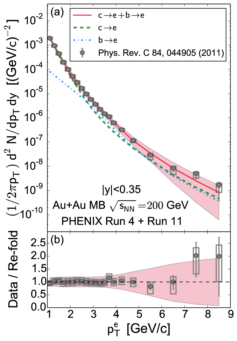
Figure 12: (Color Online) The heavy flavor electron invariant yield as a function of $p_{T}$ from measured data Adare et al. (2011) compared to electrons from the re-folded charm and bottom hadron yields. The boxes represent the point-to-point correlated uncertainties on the measured heavy flavor electron invariant yield, while the error bars on the points represent the point-to-point uncorrelated uncertainties. The label “PHENIX Run 4 + Run 11” on this and all subsequent plots indicates that the unfolding result uses the heavy flavor electron invariant yield as a function of $p_{T}$ from data taken in 2004 (Run 4) combined with $\mathrm{DCA}_{T}$ measurements from data taken in 2011 (Run 11).

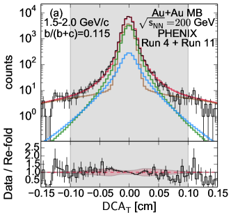
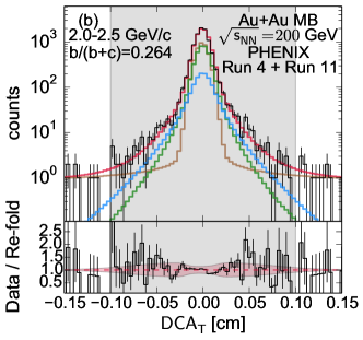
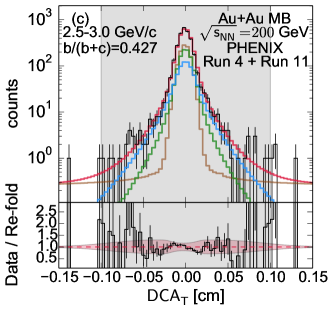
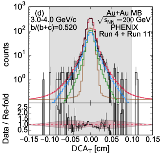
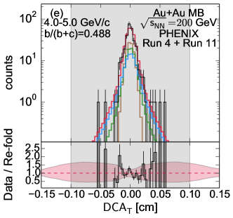
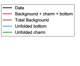
Figure 13: (Color Online) The $\mathrm{DCA}_{T}$ distribution for measured electrons compared to the decomposed $\mathrm{DCA}_{T}$ distributions for background components, electrons from charm decays, and electrons from bottom decays. The sum of the background components, electrons from charm and bottom decays is shown as the red (upper) curve for direct comparison to the data. The gray band indicates the region in $\mathrm{DCA}_{T}$ considered in the unfolding procedure. Also quoted in the figure is the bottom electron fraction for $|\mbox{$\mathrm{DCA}_{T}$}|<0.1$ cm integrated over the given $p_{T}$ range. The legend follows the same order from top to bottom as panel (b) at $\mbox{$\mathrm{DCA}_{T}$}=-0.1$ cm.

Table 2: The log likelihood values ($LL$) summed over each $\mathrm{DCA}_{T}$ distribution and for the comparison to the heavy flavor electron invariant yield. Also quoted is the number of data points ($N_{p}$) and the deviation from the log likelihood value expected from statistical fluctuations ($\Delta LL$), as discussed in the text, for each comparison.

Data set	$N_{p}$	LL	$\Delta LL$ [$\sigma$]
$e$ $\mathrm{DCA}_{T}$ $1.5<\mbox{$p_{T}^{e}$}<2.0$	50	-195.5	-3.8
$e$ $\mathrm{DCA}_{T}$ $2.0<\mbox{$p_{T}^{e}$}<2.5$	50	-156.5	-2.9
$e$ $\mathrm{DCA}_{T}$ $2.5<\mbox{$p_{T}^{e}$}<3.0$	50	-115.8	-0.6
$e$ $\mathrm{DCA}_{T}$ $3.0<\mbox{$p_{T}^{e}$}<4.0$	50	-104.1	-1.8
$e$ $\mathrm{DCA}_{T}$ $4.0<\mbox{$p_{T}^{e}$}<5.0$	50	-53.2	0.0
$e$ Inv. Yield. $1.0<\mbox{$p_{T}^{e}$}<9.0$	21	-45.9	-3.5
Total Sum	271	-673.8

III.8 Systematic uncertainties

When performing the unfolding procedure, only the statistical uncertainties on the electron $\mathrm{DCA}_{T}$ and $p_{T}$ spectra are included. In this section we describe how we consider the systematic uncertainties on both the measured data and the unfolding procedure. We take the following uncertainties into account as uncorrelated uncertainties:

1. Systematic uncertainty in the heavy flavor electron $p_{T}$ invariant yield

2. Uncertainty in the high-multiplicity background

3. Uncertainty in the fraction of nonphotonic electrons ($F_{\rm NP}$)

4. Uncertainty in $K_{e3}$ normalization

5. Regularization hyperparameter $\alpha$

6. Uncertainty in the form of $\boldsymbol{\theta}_{{\rm prior}}$

The uncertainty in $F_{\rm NP}$ (See Sec. VI.1), and $K_{e3}$ are propagated to the unfolded hadron yields by varying each independently by $\pm 1\sigma$, and performing the unfolding procedure with the modified background template. The difference between the resulting hadron yields and the central values is taken as the systematic uncertainty. The same procedure is used to determine the uncertainty in the result due to the regularization parameter, which is varied by ${}^{+0.60}_{-0.25}$ based on where the summed likelihood from both the data and regularization drops by 1 from the maximum value.

The uncertainty in the high-multiplicity background includes two components. The first is the uncertainty on the normalization of the high-multiplicity background $\mathrm{DCA}_{T}$ distribution, as determined in Sec. III.5.2 and shown in Fig. 5. This is propagated to the unfolded hadron yields by varying the normalization by $\pm 1\sigma$ and performing the unfolding procedure with the modified background template, as with the $F_{\rm NP}$ and $K_{e3}$ uncertainties. The second component addresses the small excess in the embedded primary electron distribution observed in Fig. 6 and not accounted for by using the $\mathrm{DCA}_{T}$ distribution for large $\mathrm{DCA}_{L}$. We parametrize the excess, which is more than two orders of magnitude below the peak, and apply it to the background components, re-performing the unfolding procedure to find its effect on the hadron yield. Both effects combined are small relative to the dominant uncertainties.

Incorporating the $p_{T}$ correlated systematic uncertainty on the heavy flavor electron invariant yield is more difficult. Ideally one would include a full covariance matrix encoding the $p_{T}$ correlations into the unfolding procedure. In practice, the methodology employed in Adare et al. (2011) does not provide a convenient description of the $p_{T}$ correlations needed to shape the covariance matrix. Instead we take a conservative approach by considering the cases which we believe represent the maximum $p_{T}$ correlations. We modify the heavy flavor electron invariant yield by either tilting or kinking the spectrum about a given point. Tilting simply pivots the spectra about the given point so that, for instance, the first point goes up by a fraction of the systematic uncertainty while the last point goes down by the same fraction of its systematic uncertainty, with a linear interpolation in between. Kinking simply folds the spectra about the given point so that that the spectrum is deformed in the form of a V. We implement the following modifications and re-perform the unfolding procedure:

1. Tilt the spectra about $\mbox{$p_{T}$}=1.8$ GeV/$c$ by $\pm 1\sigma$ of the systematic uncertainty.

2. Tilt the spectra about $\mbox{$p_{T}$}=5$ GeV/$c$ by $\pm 1\sigma$ of the systematic uncertainty.

3. Kink the spectra about $\mbox{$p_{T}$}=1.8$ GeV/$c$ by $\pm 1\sigma$ of the systematic uncertainty.

4. Kink the spectra about $\mbox{$p_{T}$}=5$ GeV/$c$ by $\pm 1\sigma$ of the systematic uncertainty.

The $p_{T}$ points about which the spectra were modified were motivated by the points in $p_{T}$ at which analysis methods and details changed, as discussed in Adare et al. (2011). We then take the RMS of the resulting deviations on the hadron yield from the central value as the propagated systematic uncertainty due to the systematic uncertainty on the heavy flavor electron invariant yield.

The effect of our choice of $\boldsymbol{\theta}_{{\rm prior}}$ on the charm and bottom hadron yields is taken into account by varying $\boldsymbol{\theta}_{{\rm prior}}$, as discussed in Section III.7.5. The differences between each case and the central value are added in quadrature to account for the bias introduced by $\boldsymbol{\theta}_{{\rm prior}}$.

The uncertainties on the unfolded hadron yields due to the six components described above and the uncertainty determined from the posterior probability distributions are added in quadrature to give the uncertainty shown in Fig. 15.

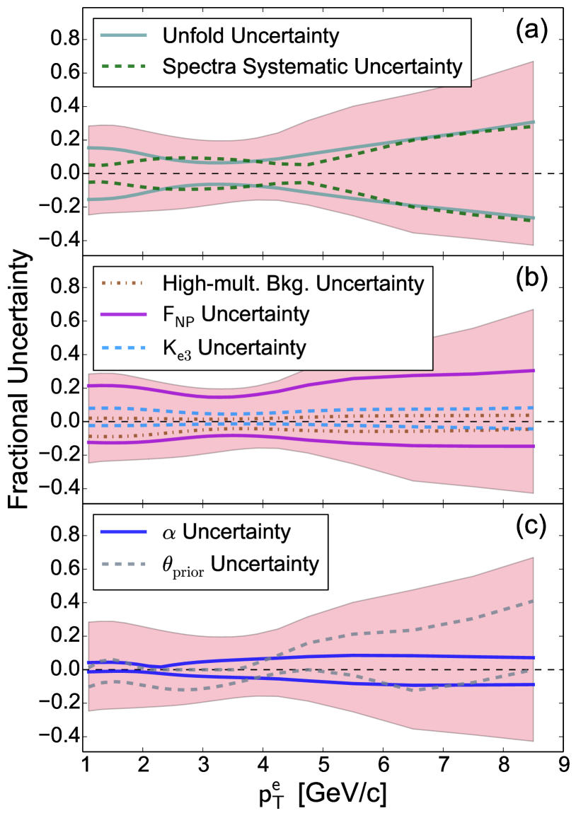
Figure 14: (Color Online) The relative contributions from the different components to the uncertainty on the fraction of electrons from bottom hadron decays as a function of $p_{T}$. The shaded red band in each panel is the total uncertainty.

Due to the correlations between charm and bottom yields, the relative contributions from the different uncertainties depend on the variable being plotted. To give some intuition for this, we have plotted the relative contributions from the different uncertainties to the fraction of electrons from bottom hadron decays as a function of $p_{T}$ (discussed in Sec. IV.1) in Fig. 14. One can see that the dominant uncertainties come from the statistical uncertainty on the $\mathrm{DCA}_{T}$ and heavy flavor electron invariant yield, the systematic uncertainty on the heavy flavor electron invariant yield, and $F_{\rm NP}$. We remind the reader that for $\mbox{$p_{T}$}>5$ GeV/$c$ we no longer have $\mathrm{DCA}_{T}$ information to directly constrain the unfolding, and all information comes dominantly from the heavy flavor electron invariant yield, leading to the growth in the uncertainty band in this region.

IV Results

The final result of the unfolding procedure applied simultaneously to the heavy flavor electron invariant yield vs $p_{T}$ (shown in Fig. 12) and the five electron $\mathrm{DCA}_{T}$ distributions (shown in Fig. 13) is the invariant yield of charm and bottom hadrons, integrated over all rapidity, as a function of $p_{T}$. As a reminder, the hadron yields are integrated over all rapidity by assuming the rapidity distribution within pythia is accurate and that it is unmodified in Au$+$Au, as detailed in Sec. III.7.4. The unfolded results for MB (0%–96%) Au$+$Au collisions at $\sqrt{s_{{}_{NN}}}$ =200 GeV are shown in Fig. 15. The central point represents the most likely value and the shaded band represents the $1\sigma$ limits on the combination of the uncertainty in the unfolding procedure and the systematic uncertainties on the data, as described in Sec. III.8. The uncertainty band represents point-to-point correlated uncertainties, typically termed Type B in PHENIX publications. There are no point-to-point uncorrelated (Type A), or global scale uncertainties (Type C), from this procedure.

The uncertainties on the hadron invariant yields shown in Fig. 15 grow rapidly for charm and bottom hadrons with $\mbox{$p_{T}$}>6$ GeV/$c$. This is due to the lack of $\mathrm{DCA}_{T}$ information for $\mbox{$p_{T}^{e}$}>5$ GeV/$c$. Above $\mbox{$p_{T}^{e}$}>5$ GeV/$c$, the unfolding is constrained by the heavy flavor electron invariant yield only. This provides an important constraint on the shape of the hadron $p_{T}$ distributions, but the $\mathrm{DCA}_{T}$ distributions provide the dominant source of discriminating power between the charm and bottom. However, due to the decay kinematics, even high $p_{T}$ hadrons contribute electrons in the range $1.5<\mbox{$p_{T}^{e}$}\ [{\rm~{}GeV}/c]<5.0$. We find that charm(bottom) hadrons in the range $7<\mbox{$p_{T}^{h}$}\ [{\rm~{}GeV}/c]<20$ contribute 18.2%(0.3%) of the total electron yield in the region $1.5<\mbox{$p_{T}^{e}$}\ [{\rm~{}GeV}/c]<5.0$. This explains the larger uncertainties in the bottom hadron yield compared to the charm hadron yield at high $p_{T}^{h}$.

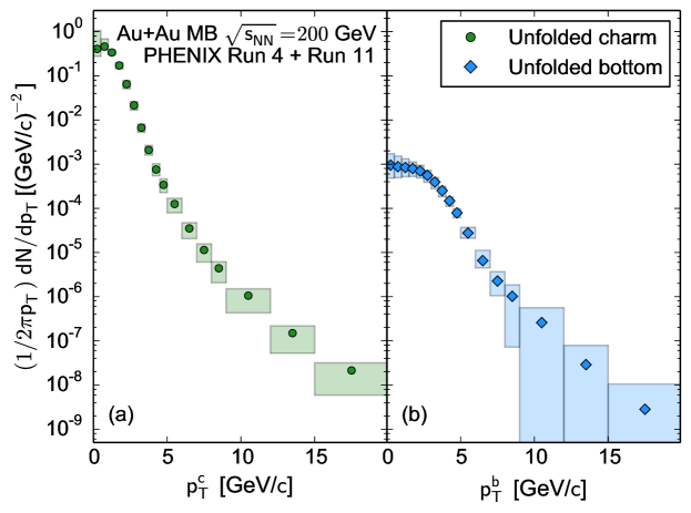
Figure 15: (Color Online) Unfolded (a) charm and (b) bottom hadron invariant yield as a function of $p_{T}$, integrated over all rapidities, as constrained by electron yield vs $\mathrm{DCA}_{T}$ in 5 $p_{T}^{e}$ bins and previously published heavy flavor electron invariant yield vs $p_{T}^{e}$ Adare et al. (2011).

The yield of $D^{0}$ mesons over $|y|<1$ as a function of $p_{T}$ has been previously published in Au$+$Au collisions at $\sqrt{s_{{}_{NN}}}$ =200 GeV by STAR Adamczyk et al. (2014). In order to compare our unfolded charm hadron results over all rapidity to the STAR measurement, we use pythia to calculate the fraction of $D^{0}$ mesons within $|y|<1$ compared to charm hadrons over all rapidity. Since the measurement by STAR is over a narrower centrality region (0%–80% vs 0%-96%), we scale the STAR result by the ratio of the $N_{\rm coll}$ values. This comparison is shown in Fig. 16. For added clarity, we have fit the STAR measurement with a Levy function modified by a blast wave calculation given by

$$f(p_{T}) = p_{0}\left(1-\frac{(1-p_{1})p_{T}}{p_{2}}\right)^{1/(1-p_{1})}$$

$$\times \left(1.3\sqrt{2\pi p_{4}^{2}}G(p_{T},p_{3},p_{4})+\frac{p_{5}}{1+e^{-p_{T}+3}}\right),$$

where $G(p_{T},p_{3},p_{4})$ is a standard Gaussian function, and $p_{i}$ are the parameters of the fit. The ratio of the data to the fit is shown in the bottom panel of Fig. 16. We find that, within uncertainties, the unfolded $D^{0}$ yield agrees with that measured by STAR over the complementary $p_{T}$ range. The unfolded yield hints at a different trend than the STAR data for $\mbox{$p_{T}$}>5$ GeV/$c$. However, we note that the $\langle\mbox{$p_{T}$}\rangle$ of charm(bottom) hadrons which contribute electrons in the range $4.0<\mbox{$p_{T}$}\ [{\rm~{}GeV}/c]<5.0$ is 7.2(6.4) GeV/$c$. This means that the yields of charm and bottom hadrons have minimal constraint from the $\mathrm{DCA}_{T}$ measurements in the high-$p_{T}$ regions, which is represented by an increase in the uncertainties.

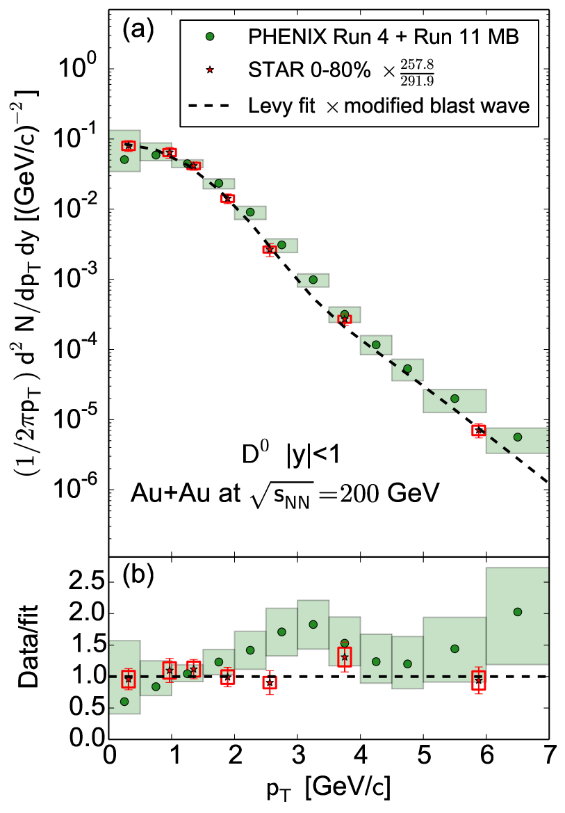
Figure 16: (Color Online) The invariant yield of $D^{0}$ mesons as a function of $p_{T}$ for $|y|<1$ inferred from the unfolded yield of charm hadrons integrated over all rapidity compared to measurements from STAR Adamczyk et al. (2014). See the text for details on the calculation of the $D^{0}$ yield inferred from the unfolded result. To match the centrality intervals, the STAR result has been scaled by the ratio of $N_{\rm coll}$ values. The bottom panel shows the ratio of the data to a fit of the STAR $D^{0}$ yield.

IV.1 The bottom electron fraction

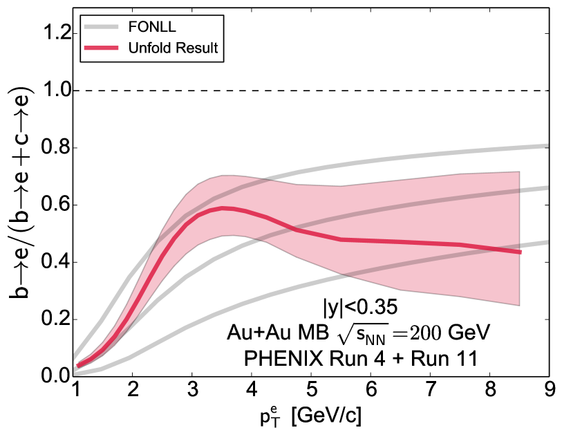
Figure 17: (Color Online) The fraction of heavy flavor electrons from bottom hadron decays as a function of $p_{T}$ from this work and from fonll $p$$+$$p$ calculations Cacciari et al. (2005).

The fraction of heavy flavor electrons from bottom hadrons ($\frac{b\rightarrow e}{b\rightarrow e+c\rightarrow e}$) is computed by re-folding the charm and bottom hadron yields shown in Fig. 15 to get the invariant yield of electrons from charm and bottom decays at midrapidity ($|y|<0.35$). Here the electrons from bottom hadron decays include the cascade decay $b\rightarrow c\rightarrow e$. The resulting bottom electron fraction is shown as a function of $p_{T}$ in Fig. 17. The central values integrated over the $p_{T}$ range of each $\mathrm{DCA}_{T}$ distribution are also quoted in Fig. 13. As in the hadron yields, the band represents the $1\sigma$ limits of the point-to-point correlated (Type B) uncertainties.

Also shown in Fig. 17 is the bottom electron fraction predictions from fonll Cacciari et al. (2005) for $p$$+$$p$ collisions at $\sqrt{s_{{}_{NN}}}$ =200 GeV. We find a bottom electron fraction which is encompassed by the fonll calculation uncertainties. The shape of the resulting bottom electron fraction shows a steeper rise in the region $2.0<\mbox{$p_{T}$}\ [{\rm GeV}/c]<4.0$ with a possible peak in the distribution compared to the central fonll calculation.

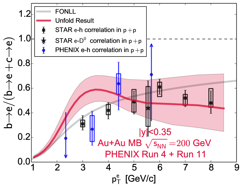
Figure 18: (Color Online) bottom electron fraction as a function of $p_{T}$ compared to measurements in $p$$+$$p$ collisions at $\sqrt{s}$ =200 GeV from PHENIX Adare et al. (2009) and STAR Aggarwal et al. (2010). Also shown are the central values for fonll Cacciari et al. (2005) for $p$$+$$p$ collisions at $\sqrt{s_{{}_{NN}}}$ =200 GeV.

The fraction of electrons from bottom decays has been previously measured in $p$$+$$p$ collisions at $\sqrt{s_{{}_{NN}}}$ =200 GeV by both PHENIX Adare et al. (2009) and STAR Aggarwal et al. (2010). These measurements are made through electron-hadron or electron-$D$ meson correlations. These are very different analyses than the one presented here, and have their own model dependencies. In Fig. 18 we compare the bottom electron fraction between our unfolded Au$+$Au result and the electron-hadron correlation measurements in $p$$+$$p$. For $\mbox{$p_{T}$}>4$ GeV/$c$ we find agreement between Au$+$Au and $p$$+$$p$ within the large uncertainties on both measurements. This implies that electrons from bottom hadron decays are similarly suppressed to those from charm. For reference, included in Fig. 18 is the central fonll calculation which, within the large uncertainties, is consistent with the $p$$+$$p$ measurements.

With the additional constraints on the bottom electron fraction in $p$$+$$p$ from the correlation measurements and the measured nuclear modification of heavy flavor electrons, we can calculate the nuclear modification of electrons from charm and bottom hadron decays separately. The nuclear modifications, $R_{AA}^{c\rightarrow e}$ and $R_{AA}^{b\rightarrow e}$, for charm and bottom hadron decays respectively are calculated using

$$R_{AA}^{c\rightarrow e} =\frac{(1-F_{\rm AuAu})}{(1-F_{pp})}R_{AA}^{\rm HF}$$ (11)

$$R_{AA}^{b\rightarrow e} =\frac{F_{\rm AuAu}}{F_{pp}}R_{AA}^{\rm HF},$$ (12)

where $F_{\rm AuAu}$ and $F_{pp}$ are the fractions of heavy flavor electrons from bottom hadron decays in Au$+$Au and $p$$+$$p$ respectively and $R_{AA}^{\rm HF}$ is the nuclear modification of heavy flavor electrons (combined charm and bottom). Rather than combining all measurements for the bottom electron fraction in $p$$+$$p$, which introduces a further extraction uncertainty, we have chosen to calculate $R_{AA}^{c\rightarrow e}$ and $R_{AA}^{b\rightarrow e}$ using only the six STAR electron-hadron $F_{pp}$ values. When performing the calculation we determine the full probability distributions assuming Gaussian uncertainties on $F_{\rm AuAu}$, $F_{pp}$ and $R_{AA}^{\rm HF}$. As when determining the charm and bottom hadron yields, we take the median of the distribution as the central value, and the 16% and 84% of the distribution as the lower and upper $1\sigma$ uncertainties. The resulting values are shown in Fig. 19(a). We find that the electrons from bottom hadron decays are less suppressed than electrons from charm hadron decays for $3<\mbox{$p_{T}$}\ \mbox{GeV/$c$}<4$. To further clarify this statement, we calculate the ratio of $R_{AA}^{b\rightarrow e}/R_{AA}^{c\rightarrow e}$, shown in Fig. 19(b). In this ratio, the uncertainty on $R_{AA}^{\rm HF}$ cancels. Here again we calculate the full probability distributions and use the same procedure as above to determine the central values and uncertainties. We find that the probability distributions for $R_{AA}^{b\rightarrow e}/R_{AA}^{c\rightarrow e}$ are highly nonGaussian, which leads to the large asymmetric uncertainty band shown in Fig. 19(b). It is clear from the ratio that $b\rightarrow e$ is less suppressed than $c\rightarrow e$ at the $1\sigma$ level up to $\mbox{$p_{T}$}\sim 4$ GeV/$c$.

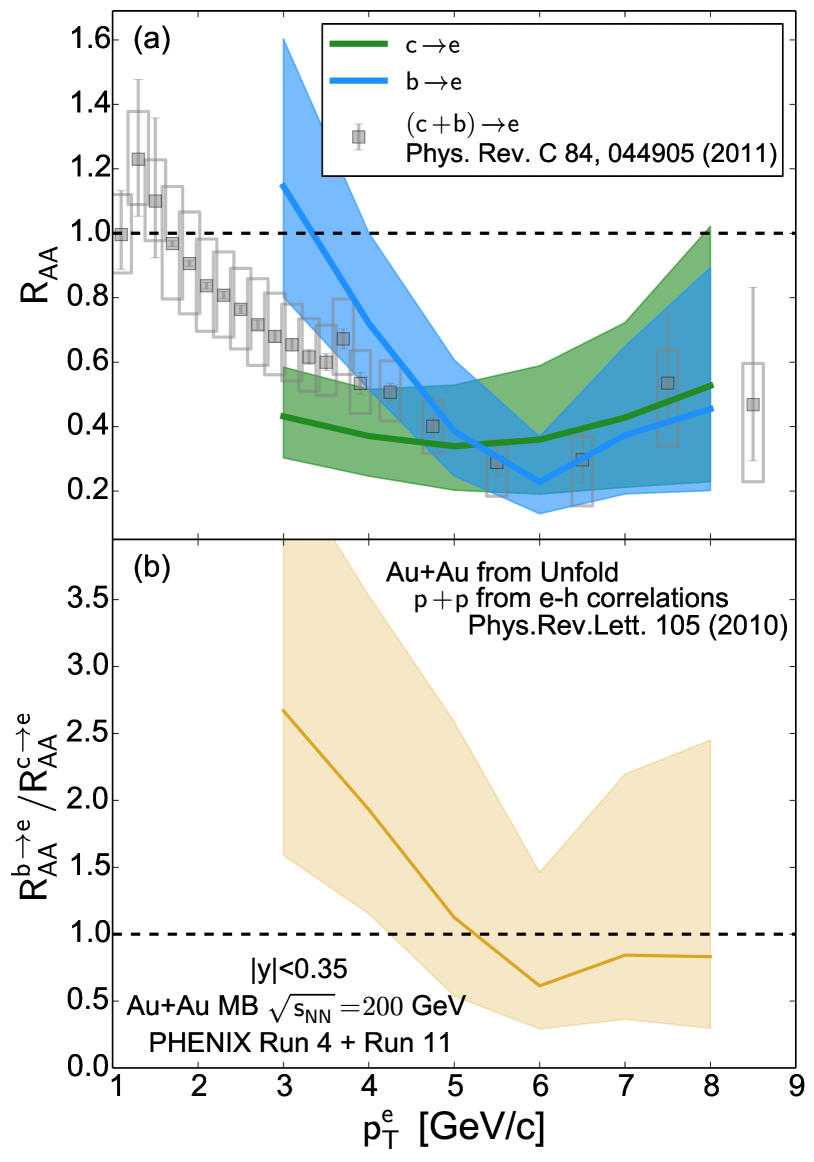
Figure 19: (Color Online) (a) The $R_{AA}$ for $c\rightarrow e$, $b\rightarrow e$ and combined heavy flavor Adare et al. (2011) as a function of $p_{T}^{e}$. The $c\rightarrow e$ and $b\rightarrow e$ $R_{AA}$ is calculated using Eq. 11-12 where $F_{\rm AuAu}$ uses the unfolded result determined in this work and $F_{pp}$ determined from STAR $e-h$ correlations Aggarwal et al. (2010). (b) The ratio $R_{AA}^{b\rightarrow e}/R_{AA}^{c\rightarrow e}$ as a function of $p_{T}^{e}$.

V Discussion

There are a number of theoretical calculations in the literature for the interaction of charm and bottom quarks with the QGP. Many of these models have predictions for the nuclear modification factor $R_{AA}$ for electrons from charm decays and, separately, $R_{AA}$ for electrons from bottom decays. For consistency, we have assumed the fonll Cacciari et al. (2005) yields for electrons from charm (bottom) decays calculated for $p$$+$$p$ at $\sqrt{s_{{}_{NN}}}$ =200 GeV and then scaled them by the heavy-ion model results for the $R_{AA}$ of electrons from charm (bottom).

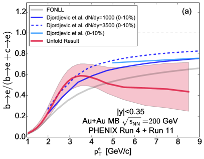
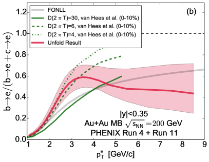
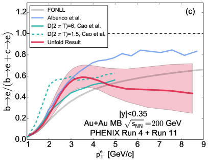
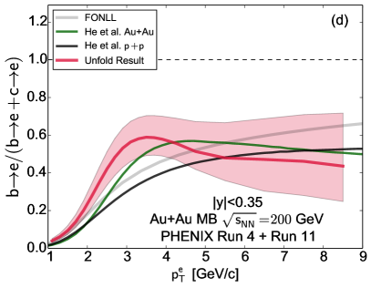
Figure 20: (Color Online) Bottom electron fraction as a function of $p_{T}$ compared to a series of model predictions detailed in the text.

Figure 20(a) compares the bottom electron fraction from one class of calculations modeling only energy loss of these heavy quarks in medium. In an early pQCD calculation by Djordjevic, Gyulassy, Vogt, and Wicks Djordjevic et al. (2006), the authors apply the DGLV theory of radiative energy loss. They find that even for extreme opacities with gluon rapidity densities up to 3500, the bottom quark decay electrons dominate at high-$p_{T}$ and that limits the single electron $R_{AA}$ to the range $0.5$–$0.6$ for $\mbox{$p_{T}$}>5$ GeV/$c$. Although this result is known to be higher than the PHENIX measured heavy flavor electron $R_{AA}$ Adare et al. (2011), we show the $b\rightarrow e/(b\rightarrow e+c\rightarrow e)$ predictions for gluon rapidity densities of 1000 and 3500 in Fig. 20(a). However, we do note that the calculations are for 0%–10% central collisions compared to the MB data, although the calculations span a factor of 3.5 range in the gluon density. We find that the calculations for both gluon rapidity densities are in good agreement with our results for $\mbox{$p_{T}$}<4$ GeV/$c$, but are slightly above and outside the uncertainty band on the unfolded result at higher $p_{T}$. More recent calculations in the same framework, but with the inclusion of collisional energy loss Djordjevic and Djordjevic (2014), result in a heavy flavor electron high-$p_{T}$ $R_{AA}$ closer to 0.3 and in reasonable agreement with previous PHENIX published results Adare et al. (2011). This updated prediction for the bottom electron fraction, also shown in Fig. 20, gives a similar value to their previous result, but is only published for $\mbox{$p_{T}$}>5$ GeV/$c$.

Figure 20(b) compares the bottom electron fraction from a calculation using a T-matrix approach by van Hees, Mannarelli, Greco, and Rapp van Hees et al. (2009). The authors provided us with different results for 0%–10% central Au$+$Au collisions depending on the coupling of the heavy-quark to the medium. The coupling is encapsulated in the diffusion parameter $D$, where smaller values yield a stronger coupling. Shown in Fig. 20(b) are three results corresponding to three values of the parameter $D(2\pi T)=4,6,30$. The largest $D$ value, corresponding to the weakest coupling, yields almost no deviation from the $p$$+$$p$ reference fonll result, and the successively stronger coupling pushes the bottom fraction contribution higher and higher. We find that the calculations with $D(2\pi T)=4,6$ are in good agreement with our result for $\mbox{$p_{T}$}<4$ GeV/$c$, but begin to diverge where the calculation stops at 5 GeV/$c$.

Figure 20(c) compares the bottom electron fraction from another class of calculations which employ a combination of Langevin, or transport type modeling of heavy-quarks, in the bulk QGP with energy loss mechanisms that dominate at higher $p_{T}$. In Ref. Alberico et al. (2011), Alberico et al. employ a Langevin calculation where a good match to the PHENIX heavy flavor electrons is found. It is notable that this calculation has a very strong suppression of charm decay electrons such that bottom contributions dominate even at modest $p_{T}$ $\geq$ 2 GeV/$c$. The calculations are consistent with the data for $\mbox{$p_{T}$}<4$ GeV/$c$ and over-predict the bottom contribution for higher $p_{T}$ values.

Figure 20(c) also compares the bottom electron fraction from another variant of the Langevin calculation by Cao et al., as detailed in Ref. Cao et al. (2013b). For this calculation, we show two results corresponding to two different input values $D(2\pi T)=1.5$ and 6. For the lower parameter, again stronger heavy-quark to medium coupling, there is a sharp rise in the bottom contribution which then flattens out. This feature is due to the increased collisional energy loss, which has a larger effect on the charm quarks, coupled with the strong radial flow effects enabling the heavier bottom quarks to dominate even at $\mbox{$p_{T}$}\sim 2$ GeV/$c$. These calculations use an impact parameter of $b=6.5$ fm, which should roughly correspond to MB collisions. We find that the calculation using the larger value of $D(2\pi T)=6.0$ is in reasonable agreement with the data across the calculated $p_{T}$ range.

Lastly, Fig. 20(d) shows a more recent calculation by He et al. employing a T-matrix approach similar to that shown in Fig. 20(b), but with a number of updates as described in Ref. He et al. (2014). In this case the authors provided a calculation of the bottom electron fraction in both $p$$+$$p$ and Au$+$Au at $\sqrt{s_{{}_{NN}}}$ =200 GeV, and we therefore do not calculate the bottom fraction using fonll as a baseline. The calculation is performed for the 20%–40% centrality bin, which the authors find well represents MB. We find that the calculation under-predicts the bottom fraction for $\mbox{$p_{T}$}<3$ GeV/$c$, although it is worth noting that the calculation in $p$$+$$p$ is also below the fonll curve across the full $p_{T}$ range. Above $\mbox{$p_{T}$}\sim 3$ GeV/$c$ the calculation is in agreement with the measurement. It is also worth noting that, of the models presented here, this is the only one that shows in Au$+$Au a slight decrease in the bottom fraction at high $p_{T}$.

There are numerous other calculations in the literature Vitev et al. (2007); Horowitz (2015, 2009) that require mapping charm and bottom hadrons to electrons at midrapidity to make direct data comparisons. We look forward to soon being able to test these calculations with analysis of new PHENIX data sets.

VI Summary and Conclusions

This article has detailed the measurements of electrons as a function of $\mathrm{DCA}_{T}$ and $p_{T}$ from Au$+$Au data taken at $\sqrt{s_{{}_{NN}}}$ =200 GeV in 2011 with the enhanced vertexing capabilities provided by the VTX detector. In conjunction with previous PHENIX results for the heavy flavor electron invariant yield as a function of $p_{T}$ Adare et al. (2011), we perform an unfolding procedure to infer the parent charm and bottom hadron yields as a function of $p_{T}$. We find that this procedure yields consistent agreement between the heavy flavor electron invariant yield and the newly measured electron $\mathrm{DCA}_{T}$ distributions.

We find that the extracted $D^{0}$ yield vs $p_{T}$ is in good agreement with that measured by STAR Adamczyk et al. (2014) over the complimentary $p_{T}$ region. Without a proper $p$$+$$p$ baseline extracted from a similar analysis it is difficult to make any quantitative statements about the charm or bottom hadron modification.

We compare the extracted bottom electron fraction to measurements in $p$$+$$p$ collisions and find agreement between Au$+$Au and $p$$+$$p$ for $\mbox{$p_{T}$}>4$ GeV/$c$ within the large uncertainties on both measurements. The agreement between Au$+$Au and $p$$+$$p$ coupled with the measured heavy flavor electron $R_{AA}$ strongly implies that electrons from charm and bottom hadron decays are suppressed. Using these components we calculate the nuclear modification for electrons from charm and bottom hadron decays and find that electrons from bottom hadron decays are less suppressed than those from charm hadron decays in the range $3<\mbox{$p_{T}$}\ \mbox{GeV/$c$}<4$. We further compare the bottom electron fraction to a variety of model calculations employing variously energy loss, Langevin transport, and T-matrix approaches. We find that there are a number of models which are in reasonable agreement with the extracted bottom electron fraction within the relatively large uncertainties.

We note that a significantly larger data set of Au$+$Au collisions at $\sqrt{s_{{}_{NN}}}$ =200 GeV was collected in 2014 with an improved performance of the VTX detector. The 2014 Au$+$Au data coupled with the $p$$+$$p$ data taken in 2015 should yield both an important baseline measurement of the bottom electron fraction and a more precise measurement in Au$+$Au.

APPENDIX: Detailed Normalization of electron background components

This appendix details the calculation of the normalizations for the background components:

• Photonic electrons

• Kaon decay electrons

• Heavy quarkonia decay electrons

using the bootstrap method described in Sec. III.6. We first determine the fraction of nonphotonic electrons, $F_{\rm NP}$. We then calculate the normalization of Dalitz and conversion components followed by the normalization of $K_{e3}$ and quarkonia components.

VI.1 Fraction of nonphotonic electrons $F_{\rm NP}$

We first determine $F_{\rm NP}$, the fraction of nonphotonic electrons to inclusive electrons after the application of all analysis cuts, including the conversion veto cut. Note that nonphotonic electrons include contributions from heavy flavor semi-leptonic decays, quarkonia decays, and kaon decays. Photonic electrons are from $\pi^{0}$ and $\eta$ Dalitz decays and photon conversions.

$F_{\rm NP}$ in the 2011 data can be determined using the published 2004 result Adare et al. (2011) as follows. Let $Y_{\rm NP}$ be the yield of nonphotonic electrons and $Y_{Dalitz}$ the yield of electrons from Dalitz decays. Note that both $Y_{\rm NP}$ and $Y_{Dalitz}$ are independent of the year of data taking. In the PHENIX 2004 Au$+$Au data run, the ratio of the nonphotonic electron yield to the photonic electron yield ($R_{\rm NP}^{2004}$) was measured. The relation of $Y_{\rm NP}$ and $Y_{Dalitz}$ is as follows:

$$Y_{\rm NP}=R_{\rm NP}^{2004}(1+R^{2004}_{CD})\times Y_{Dalitz},$$ (13)

where $R^{2004}_{CD}$ represents the ratio of conversion electron yield to Dalitz electron yield in the 2004 PHENIX detector. It is calculated as

$$R^{2004}_{CD}=\sum_{i=\pi^{0},\eta,\gamma}R_{CD}^{2004}(i)\cdot r_{Dalitz}(i)).$$ (14)

Here $R_{CD}^{2004}(i)$ is the ratio of conversion electrons to electrons from Dalitz decays in the 2004 PHENIX detector calculated by a full geant3 simulation. The factors

• $r_{Dalitz}(\pi^{0})$

• $r_{Dalitz}(\eta)$

• $r_{Dalitz}(\gamma)$

are the fractional contributions of $\pi^{0}$, $\eta$, and direct photon contribution to the total Dalitz decays, respectively. We only consider the contributions of $\pi^{0}$, $\eta$, and $\gamma_{dir}$ (direct photon) since the sum of other contributions is small (5% or less). Thus they are normalized such that

$$\sum_{i}r_{Dalitz}(i)=1.$$ (15)

Figure 21 shows $r_{Dalitz}$ for $\pi^{0}$, $\eta$, and direct photon as a function of transverse momentum of the electrons for MB Au$+$Au collisions at 200 GeV. The ratios are calculated from the invariant yield of $\pi^{0}$Adare et al. (2008), $\eta$Adare et al. (2010b), and direct photonsAfanasiev et al. (2012); Adare et al. (2010a).

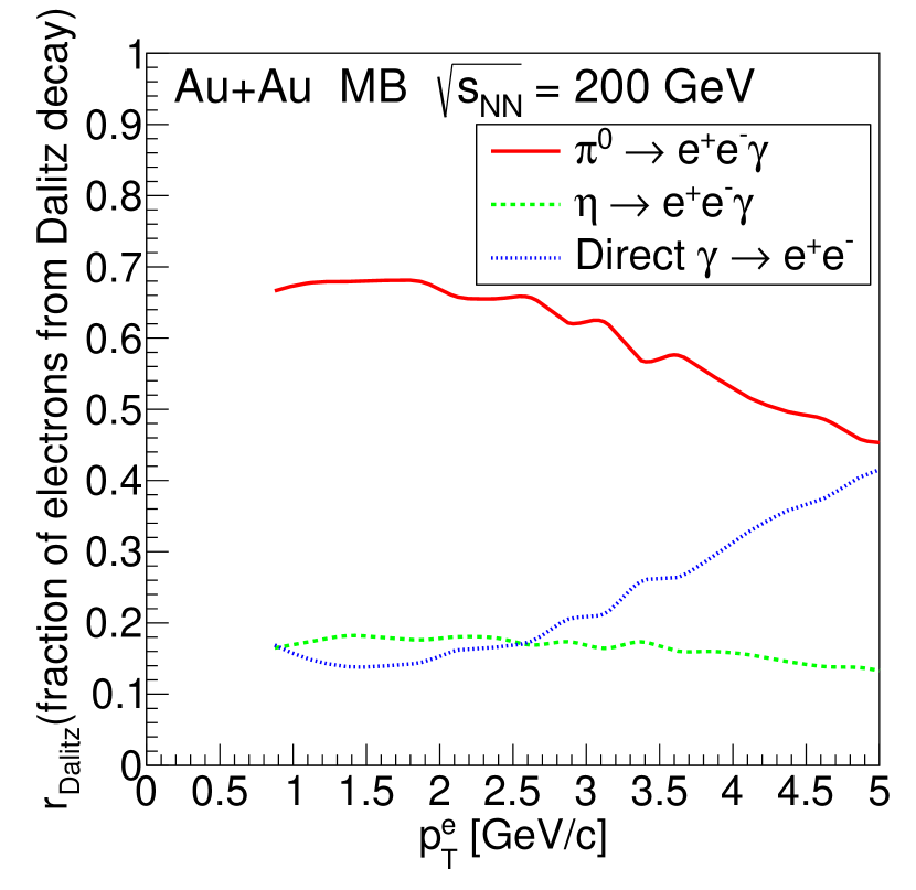
Figure 21: (Color Online) The fraction of $\pi^{0}$, $\eta$, and direct photon Dalitz decay electrons in all Dalitz electrons as a function of electron $p_{T}$ ($p_{T}^{e}$).

In the 2011 data set the observed electron yields from conversion and Dalitz decays are modified by the electron survival probability after the conversion veto cut is applied. The yield of photonic electrons which pass the conversion veto $(Y_{P}^{2011})$ is

$$Y_{P}^{2011} = R^{2011}_{PD}\times Y_{Dalitz},$$ (16)

$$R^{2011}_{PD} = \sum_{i=\pi^{0},\eta,\gamma}\left(S_{D}(i)+S_{C}\cdot R_{CD}^{2011}(i)\right)r_{Dalitz}(i),$$ (17)

where $S_{C}$ is the survival probability of conversion electrons, $S_{D}(\pi^{0}),S_{D}(\eta),S_{D}(\gamma)$ are survival probabilities of Dalitz decay electrons from $\pi^{0}$, $\eta$, and direct photons, respectively, as shown in Fig. 8. $R_{CD}^{2011}(i)$ ($i=\pi^{0},\eta,\gamma$)is the ratio of conversion electrons to Dalitz electrons for particle $i$ in the 2011 PHENIX detector after the addition of the VTX and the replacement of the beam pipe. It is determined to be $R_{CD}^{2011}(i)\approx 1.10$ from full geant3 simulations.

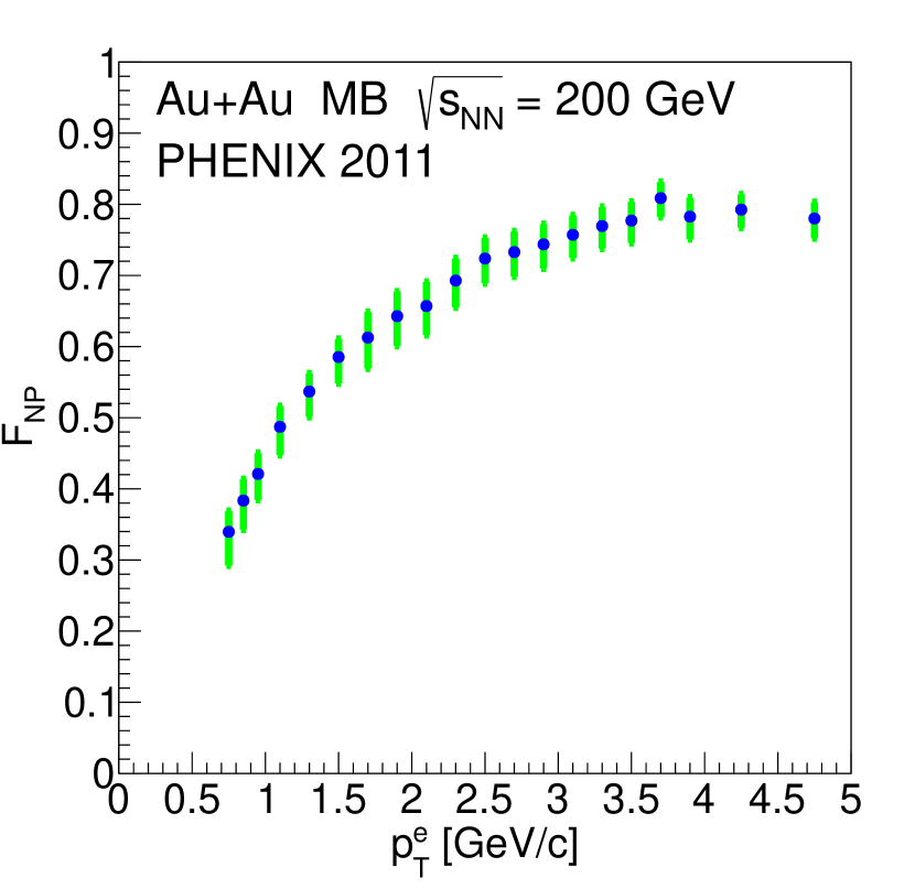
Figure 22: (Color Online) The fraction of nonphotonic electrons to inclusive electrons as a function of electron $p_{T}$ ($p_{T}^{e}$).

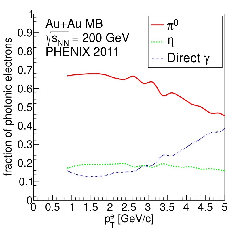
Figure 23: (Color Online) The fraction of $\pi^{0}$, $\eta$, and direct photon electrons in all photonic electrons as a function of electron $p_{T}$ ($p_{T}^{e}$).

The fraction of nonphotonic electrons to inclusive electrons can then be calculated as

$$F_{\rm NP} = \frac{Y_{\rm NP}}{Y_{\rm NP}+Y_{P}^{2011}}$$ (18)

$$= \frac{R^{2004}_{\rm NP}(1+R^{2004}_{CD})}{R^{2004}_{\rm NP}(1+R^{2004}_{CD})+R^{2011}_{PD}}$$ (19)

The resulting $F_{\rm NP}$ as a function of $p_{T}^{e}$ and the calculated systematic uncertainties due to the uncertainties on the input yields is shown in Fig. 22. With $F_{\rm NP}$ in hand, we obtain the number of photonic electrons, $N^{e}_{P}$, and the number of nonphotonic electrons, $N^{e}_{\rm NP}$ as

$$N_{P}^{e} = N_{e}(1-F_{\rm NP})$$ (20)

$$N_{\rm NP}^{e} = N_{e}F_{\rm NP},$$ (21)

where $N^{e}$ is the number of electrons with conversion veto after the subtraction of the hadronic contamination and random background.

VI.2 Normalization of Dalitz and conversion components

In the previous section we obtained $N^{e}_{P}$, the number of photonic electrons in the data after the conversion veto cut. There are two components in the photonic electrons ($N_{P}^{e}$).

1. Electrons from Dalitz decays ($\pi^{0}+\eta+\gamma$)

2. Electrons from conversions in the beam pipe and B0

In the next step, we determine the normalization of Dalitz and conversions separately. This is needed since the shape of $\mathrm{DCA}_{T}$ distribution of Dalitz and conversions are different.

After application of the conversion veto cut, we have

$$N^{e}_{C}(i) = S_{C}R_{CD}^{2011}(i)(1-\delta_{random})\epsilon_{A}Y_{Dalitz},$$ (22)

$$N^{e}_{D}(i) = S_{D}(i)(1-\delta_{random})\epsilon_{A}Y_{Dalitz},$$ (23)

$$(i = \pi^{0},\eta,\gamma)$$ (24)

where $N_{C}^{e}(i)$ and $N_{D}^{e}(i)$ are the number of electrons from conversions and Dalitz from particle $i$ after the conversion veto cut, respectively; $\delta_{random}$ is the common reduction factor of tracks due to random hits in the windows of the conversion veto cut; and $\epsilon_{A}$ is the efficiency and acceptance without the conversion veto cut. Since the number of photonic electron is $N^{e}_{P}(i)=N^{e}_{D}(i)+N^{e}_{C}(i)$, the fraction of conversions and Dalitz decays in the photonic electrons are

$$\frac{N^{e}_{C}(i)}{N^{e}_{P}(i)} = \frac{S_{C}R_{CD}(i)}{S_{D}(i)+S_{C}R_{CD}^{2011}(i)},$$ (25)

$$\frac{N^{e}_{D}(i)}{N^{e}_{P}(i)} = \frac{S_{D}(i)}{S_{D}(i)+S_{C}R_{CD}^{2011}(i)},$$ (26)

The fraction of electrons from conversions ($N^{e}_{C}/N^{e}_{P}$) and Dalitz ($N^{e}_{D}/N^{e}_{P}$) is the average of these fractions, thus:

$$N^{e}_{C} = N_{P}^{e}\sum_{i=\pi^{0},\eta,\gamma}r^{ph}(i)\frac{S_{C}R_{CD}^{2011}(i)}{S_{D}(i)+S_{C}R_{CD}^{2011}(i)}$$ (27)

$$N^{e}_{D} = N_{P}^{e}\sum_{i=\pi^{0},\eta,\gamma}r^{ph}(i)\frac{S_{D}(i)}{S_{D}(i)+S_{C}R_{CD}^{2011}(i)},$$ (28)

where $r^{ph}(i),(i=\pi^{0},\eta,\gamma)$ is the relative contribution of electrons from (conversion + Dalitz decay) for particle $i$ after application of conversion veto cut. Figure 23 shows $r^{ph}(i)$ $(i=\pi^{0},\eta,\gamma)$ as a function of $p_{T}^{e}$. The conversion contributions are nearly the same for $\pi^{0},\eta$ and $\gamma$, and effectively cancel when calculating the ratio. Therefore, $r^{ph}$ (Fig. 23) is almost identical with $r_{Dalitz}$ (Fig. 21).

VI.3 Normalization of $K_{e3}$ and quarkonia components

The ratio of electrons from kaons to all nonphotonic electrons before the application of the conversion veto cut, $\delta_{K}$, is calculated from the ratio of the nonphotonic electron yield to the electron yield from kaons Adare et al. (2011). Compared to Ref. Adare et al. (2011), we find that $\sim 50\%$ of electrons from kaon decays are removed by $\mathrm{DCA}_{T}$ and $\mathrm{DCA}_{L}$ cuts as well as the method used to subtract random background, which contains some real electrons from kaon decays.

The ratio of electrons from $J/\psi$ decays to all nonphotonic electrons before the application of the conversion veto cut, $\delta_{J/\psi}$, is taken from Ref. Adare et al. (2011). The survival rate for electrons from $J/\psi$ decays , $S_{J/\psi}$, is taken to be unity, while the survival rate for $K_{e3}$ decays, $S_{K}$, is taken to be the same value as that for electrons from charm and bottom decays (namely, $S_{\rm HF}$). See Sec. III.5.3 for details.

After application of conversion veto cut, the normalizations of these two nonphotonic electron components are described by

$$N_{J/\psi}^{e} =N_{\rm NP}^{e}\frac{\delta_{J/\psi}S_{J/\psi}}{\delta_{J/\psi}S_{J/\psi}+\delta_{K}S_{K}+(1-\delta_{J/\psi}-\delta_{K})S_{\rm HF}}$$ (29)

$$N_{K}^{e} =N_{\rm NP}^{e}\frac{\delta_{K}S_{K}}{\delta_{J/\psi}S_{J/\psi}+\delta_{K}S_{K}+(1-\delta_{J/\psi}-\delta_{K})S_{\rm HF}}$$ (30)

References

- Adcox et al. (2005) K. Adcox et al. (PHENIX Collaboration), “Formation of dense partonic matter in relativistic nucleus-nucleus collisions at RHIC: Experimental evaluation by the PHENIX Collaboration,” Nucl. Phys. A 757, 184 (2005).
- Adams et al. (2005) J. Adams et al. (STAR Collaboration), “Experimental and theoretical challenges in the search for the quark gluon plasma: The STAR Collaboration’s critical assessment of the evidence from RHIC collisions,” Nucl. Phys. A 757, 102 (2005).
- Adare et al. (2010a) A. Adare et al. (PHENIX Collaboration), “Enhanced production of direct photons in Au+Au collisions at =200 GeV and implications for the initial temperature,” Phys. Rev. Lett. 104, 132301 (2010a).
- Romatschke (2010) P. Romatschke, “New Developments in Relativistic Viscous Hydrodynamics,” Int. J. Mod. Phys. E 19, 1 (2010).
- Heinz and Snellings (2013) U. Heinz and R. Snellings, “Collective flow and viscosity in relativistic heavy-ion collisions,” Ann. Rev. Nucl. Part. Sci. 63, 123 (2013).
- Bazavov et al. (2014) A. Bazavov et al. (HotQCD), “Equation of state in ( 2+1 )-flavor QCD,” Phys. Rev. D 90, 094503 (2014).
- Kovtun et al. (2005) P. K. Kovtun, Dan T. Son, and A. O. Starinets, “Viscosity in strongly interacting quantum field theories from black hole physics,” Phys. Rev. Lett. 94, 111601 (2005).
- Gyulassy and McLerran (2005) M. Gyulassy and L. McLerran, “New forms of QCD matter discovered at RHIC,” Quark gluon plasma. New discoveries at RHIC: A case of strongly interacting quark gluon plasma. Proceedings, RBRC Workshop, Brookhaven, Upton, USA, May 14-15, 2004, Nucl. Phys. A 750, 30 (2005).
- (9) U. W. Heinz, “RHIC serves the perfect fluid: Hydrodynamic flow of the QGP,” in Proceedings, Workshop on Extreme QCD, p. 3 (2005).
- Adler et al. (2005) S. S. Adler et al. (PHENIX Collaboration), “Centrality dependence of charm production from single electrons measurement in Au + Au collisions at = 200 GeV,” Phys. Rev. Lett. 94, 082301 (2005).
- Adcox et al. (2002) K. Adcox et al. (PHENIX Collaboration), “Measurement of single electrons and implications for charm production in Au+Au collisions at (NN) = 130 GeV,” Phys. Rev. Lett. 88, 192303 (2002).
- Adare et al. (2011) A. Adare et al. (PHENIX Collaboration), “Heavy Quark Production in and Energy Loss and Flow of Heavy Quarks in Au+Au Collisions at =200 GeV,” Phys. Rev. C 84, 044905 (2011).
- Adare et al. (2007a) A. Adare et al. (PHENIX Collaboration), “Energy Loss and Flow of Heavy Quarks in Au+Au Collisions at = 200 GeV,” Phys. Rev. Lett. 98, 172301 (2007a).
- Adamczyk et al. (2014) L. Adamczyk et al. (STAR Collaboration), “Observation of Meson Nuclear Modifications in Au+Au Collisions at =200 GeV,” Phys. Rev. Lett. 113, 142301 (2014).
- Abelev et al. (2014) B. B. Abelev et al. (ALICE Collaboration), “Azimuthal anisotropy of D meson production in Pb-Pb collisions at =2.76 TeV,” Phys. Rev. C 90, 034904 (2014).
- (16) B. Abelev et al. (ALICE Collaboration), “Suppression of high transverse momentum D mesons in central Pb-Pb collisions at =2.76 TeV,” J. High Energy Phys. 09 (2012) 112.
- (17) S. Chatrchyan et al. (CMS Collaboration), “Suppression of nonprompt , prompt , and Y(1S) in PbPb collisions at =2.76 TeV,” J. High Energy Phys. 05 (2012) 063.
- Chatrchyan et al. (2014) S. Chatrchyan et al. (CMS Collaboration), “Evidence of b-Jet Quenching in PbPb Collisions at =2.76 TeV,” Phys. Rev. Lett. 113, 132301 (2014), [Erratum: Phys. Rev. Lett. 115, 029903 (2015)].
- Adare et al. (2014a) A. Adare et al. (PHENIX Collaboration), “System-size dependence of open-heavy-flavor production in nucleus-nucleus collisions at =200 GeV,” Phys. Rev. C 90, 034903 (2014a).
- Adare et al. (2012) A. Adare et al. (PHENIX Collaboration), “Cold-nuclear-matter effects on heavy-quark production in Au collisions at =200 GeV,” Phys. Rev. Lett. 109, 242301 (2012).
- Antreasyan et al. (1979) D. Antreasyan, J. W. Cronin, H. J. Frisch, M. J. Shochet, L. Kluberg, P. A. Piroue, and R. L. Sumner, “Production of hadrons at large transverse momentum in 200-GeV, 300-GeV and 400-GeV and collisions,” Phys. Rev. D 19, 764 (1979).
- Adare et al. (2015) A. Adare et al. (PHENIX Collaboration), “Heavy-quark production and elliptic flow in AuAu collisions at GeV,” Phys. Rev. C 91, 044907 (2015).
- Batsouli et al. (2003) S. Batsouli, S. Kelly, M. Gyulassy, and J. L. Nagle, “Does the charm flow at RHIC?” Phys. Lett. B 557, 26 (2003).
- Moore and Teaney (2005) G. D. Moore and D. Teaney, “How much do heavy quarks thermalize in a heavy ion collision?” Phys. Rev. C 71, 064904 (2005).
- Cao et al. (2013a) S. Cao, G.-Y. Qin, and S. A. Bass, “Heavy-quark dynamics and hadronization in ultrarelativistic heavy-ion collisions: Collisional versus radiative energy loss,” Phys. Rev. C 88, 044907 (2013a).
- (26) R. Rapp and H. van Hees, R. C. Hwa, X.-N. Wang (Ed.) Quark Gluon Plasma 4, 111 (2010) (World Scientific).
- van Hees et al. (2008) H. van Hees, M. Mannarelli, V. Greco, and R. Rapp, “Nonperturbative heavy-quark diffusion in the quark-gluon plasma,” Phys. Rev. Lett. 100, 192301 (2008).
- Gossiaux et al. (2010) P. B. Gossiaux, J. Aichelin, T. Gousset, and V. Guiho, “Competition of Heavy Quark Radiative and Collisional Energy Loss in Deconfined Matter,” Strangeness in quark matter. Proceedings, 14th International Conference, SQM 2009, Buzios, Rio de Janeiro, Brazil, September 27-October 2, 2009, J. Phys. G 37, 094019 (2010).
- Adare et al. (2014b) A. M. Adare, M. P. McCumber, James L. Nagle, and P. Romatschke, “Examination whether heavy quarks carry information on the early-time coupling of the quark-gluon plasma,” Phys. Rev. C 90, 024911 (2014b).
- Dokshitzer and Kharzeev (2001) Y. L. Dokshitzer and D. E. Kharzeev, “Heavy quark colorimetry of QCD matter,” Phys. Lett. B 519, 199 (2001).
- Djordjevic and Djordjevic (2014) M. Djordjevic and M. Djordjevic, “Heavy flavor puzzle from data measured at the BNL Relativistic Heavy Ion Collider: Analysis of the underlying effects,” Phys. Rev. C 90, 034910 (2014).
- Djordjevic (2006) M. Djordjevic, “An Overview of heavy quark energy loss puzzle at RHIC,” International Conference on Strangeness in Quark Matter (SQM2006) Los Angeles, California, March 26-31, 2006, J. Phys. G 32, S333 (2006).
- Cacciari et al. (2005) M. Cacciari, P. Nason, and R. Vogt, “QCD predictions for charm and bottom production at RHIC,” Phys. Rev. Lett. 95, 122001 (2005).
- Adare et al. (2009) A. Adare et al. (PHENIX Collaboration), “Measurement of Bottom versus Charm as a Function of Transverse Momentum with Electron-Hadron Correlations in Collisions at GeV,” Phys. Rev. Lett. 103, 082002 (2009).
- Aggarwal et al. (2010) M. M. Aggarwal et al. (STAR Collaboration), “Measurement of the Bottom contribution to nonphotonic electron production in collisions at =200 GeV,” Phys. Rev. Lett. 105, 202301 (2010).
- Adcox et al. (2003) K. Adcox et al. (PHENIX Collaboration), “PHENIX detector overview,” Nucl. Instrum. Methods Phys. Res., Sec. A 499, 469 (2003).
- Miller et al. (2007) M. L. Miller, K. Reygers, S. J. Sanders, and P. Steinberg, “Glauber modeling in high energy nuclear collisions,” Ann. Rev. Nucl. Part. Sci. 57, 205 (2007).
- (38) M. Baker et al. (PHENIX Collaboration), “Proposal for a Silicon Vertex Tracker (VTX) for the PHENIX Experiment,” BNL internal report 72204.
- Nouicer (2013) Rachid Nouicer (PHENIX Collaboration), “Probing Hot and Dense Matter with Charm and Bottom Measurements with PHENIX VTX Tracker,” Proceedings, 23rd International Conference on Ultrarelativistic Nucleus-Nucleus Collisions : Quark Matter 2012 (QM 2012), Nucl. Phys. A 904-905, 647c (2013).
- Kurosawa (2013) M. Kurosawa (PHENIX Collaboration), “Higher harmonics flow measurement of charged hadrons and electrons in wide kinematic range with PHENIX VTX tracker,” Proceedings, 23rd International Conference on Ultrarelativistic Nucleus-Nucleus Collisions : Quark Matter 2012 (QM 2012), Nucl. Phys. A 904-905, 397c (2013).
- Ichimiya et al. (2009) R. Ichimiya et al. (PHENIX Collaboration), “Status and overview of development of the Silicon Pixel Detector for the PHENIX experiment at the BNL RHIC,” J. Inst. 4, P05001 (2009), and references therein.
- Snoeys et al. (2001) W. Snoeys et al., “Pixel readout chips in deep submicron CMOS for ALICE and LHCb tolerant to 10-Mrad and beyond,” in Development and application of semiconductor tracking detectors. Proceedings, 4th International Symposium, Hiroshima, Japan, March 22-25, 2000, Vol. 466 (2001) p. 366.
- Li et al. (2004) Z. Li et al., “Novel silicon stripixel detector for PHENIX upgrade,” Frontier detectors for frontier physics. Proceedings, 9th Pisa Meeting on advanced detectors, La Biodola, Italy, May 25-31, 2003, Nucl. Instrum. Methods Phys. Res., Sec. A 518, 300 (2004).
- Nouicer et al. (2009) R. Nouicer et al. (PHENIX Collaboration), “Status and Performance of New Silicon Stripixel Detector for the PHENIX Experiment at RHIC: Beta Source, Cosmic-rays, and Proton Beam at 120 GeV,” J. Inst. 4, P04011 (2009), and references therein.
- Garcia-Sciveres et al. (2003) M. Garcia-Sciveres et al., “The SVX4 integrated circuit,” Proceedings, 11th International Workshop on Vertex Detectors (Vertex 2002), Nucl. Instrum. Methods Phys. Res., Sec. A 511, 171 (2003).
- Olive et al. (2014) K. A. Olive et al. (Particle Data Group Collaboration), “Rev. of Particle Phys.” Chin. Phys. C 38, 090001 (2014).
- (47) GEANT 3.2.1 Manual (CERN, Geneva, 1993).
- Wang and Gyulassy (1991) X.-N. Wang and M. Gyulassy, “HIJING: A Monte Carlo model for multiple jet production in , and collisions,” Phys. Rev. D 44, 3501 (1991).
- Adare et al. (2008) A. Adare et al. (PHENIX Collaboration), “Suppression pattern of neutral pions at high transverse momentum in Au + Au collisions at = 200 GeV and constraints on medium transport coefficients,” Phys. Rev. Lett. 101, 232301 (2008).
- Adare et al. (2010b) A. Adare et al. (PHENIX Collaboration), “Transverse momentum dependence of meson suppression suppression in Au+Au collisions at = 200 GeV,” Phys. Rev. C 82, 011902 (2010b).
- Afanasiev et al. (2012) S. Afanasiev et al. (PHENIX Collaboration), “Measurement of Direct Photons in Au+Au Collisions at =200 GeV,” Phys. Rev. Lett. 109, 152302 (2012).
- Adare et al. (2007b) A. Adare et al. (PHENIX Collaboration), “ Production vs Centrality, Transverse Momentum, and Rapidity in Au+Au Collisions at =200 GeV,” Phys. Rev. Lett. 98, 232301 (2007b).
- Cowan (2002) G. Cowan, “A survey of unfolding methods for particle physics,” Advanced statistical techniques in particle physics. Proceedings, Conference, Durham, UK, March 18-22, 2002, Conf. Proc. C 0203181, 248 (2002).
- (54) G. Choudalakis, “Fully Bayesian Unfolding,” ArXiv:1201.4612.
- Goodman, J. and Weare, J (2010) Goodman, J. and Weare, J, “Ensemble samplers with affine invariance,” Comm. App. Math. Comp. Sci. 5, 65 (2010).
- Foreman-Mackey et al. (2013) D. Foreman-Mackey, D. W. Hogg, D. Lang, and J. Goodman, “emcee: The MCMC Hammer,” Publ. Astron. Soc. Pac. 125, 306 (2013).
- (57) T. Sjostrand, S. Mrenna, and P. Z. Skands, “PYTHIA 6.4 Phys. and Manual,” J. High Energy Phys. 05 (2006) 026.
- Staszel (2006) P. Staszel (BRAHMS Collaboration), “Recent results from the BRAHMS experiment,” Proceedings, 18th International Conference on Ultra-Relativistic Nucleus-Nucleus Collisions (Quark Matter 2005), Nucl. Phys. A 774, 77 (2006).
- Abelev et al. (2006) B. I. Abelev et al. (STAR Collaboration), “Identified baryon and meson distributions at large transverse momenta from Au+Au collisions at = 200 GeV,” Phys. Rev. Lett. 97, 152301 (2006).
- Martinez-Garcia et al. (2008) G. Martinez-Garcia, S. Gadrat, and P. Crochet, “Consequences of a Lambda(c)/D enhancement effect on the nonphotonic electron nuclear modification factor in central heavy ion collisions at RHIC energy,” Phys. Lett. B 663, 55 (2008), [Erratum: Phys. Lett. B 666, 533 (2008)].
- Sorensen and Dong (2006) P. R. Sorensen and X. Dong, “Suppression of nonphotonic electrons from enhancement of charm baryons in heavy ion collisions,” Phys. Rev. C 74, 024902 (2006).
- Djordjevic et al. (2006) M. Djordjevic, M. Gyulassy, R. Vogt, and S. Wicks, “Influence of bottom quark jet quenching on single electron tomography of Au + Au,” Phys. Lett. B 632, 81 (2006).
- van Hees et al. (2009) H. van Hees, M. Mannarelli, V. Greco, and R. Rapp, “T-matrix approach to heavy quark diffusion in the QGP,” Proceedings, 3rd International Conference on Hard and Electromagnetic Probes of High-Energy Nuclear Collisions (Hard Probes 2008), Eur. Phys. J. C 61, 799 (2009).
- Alberico et al. (2011) W. M. Alberico, A. Beraudo, A. De Pace, A. Molinari, M. Monteno, M. Nardi, and F. Prino, “Heavy-flavour spectra in high energy nucleus-nucleus collisions,” Eur. Phys. J. C 71, 1666 (2011).
- Cao et al. (2013b) S. Cao, G.-Y. Qin, and S. A. Bass, “Model and parameter dependence of heavy quark energy loss in a hot and dense medium,” J. Phys. G 40, 085103 (2013b).
- He et al. (2014) M. He, R. J. Fries, and R. Rapp, “Heavy Flavor at the Large Hadron Collider in a Strong Coupling Approach,” Phys. Lett. B 735, 445 (2014).
- Vitev et al. (2007) I. Vitev, A. Adil, and H. van Hees, “Novel heavy flavor suppression mechanisms in the QGP,” Proceedings, 19th International Conference on Ultra-Relativistic nucleus-nucleus collisions (Quark Matter 2006), J. Phys. G 34, S769 (2007).
- Horowitz (2015) W. A. Horowitz, “Fluctuating heavy quark energy loss in a strongly coupled quark-gluon plasma,” Phys. Rev. D 91, 085019 (2015).
- Horowitz (2009) W. A. Horowitz, “Shock Treatment: Heavy Quark Energy Loss in a Novel AdS/CFT Geometry,” Proceedings, 21st International Conference on Ultra-Relativistic nucleus nucleus collisions (Quark matter 2009), Nucl. Phys. A 830, 773C (2009).