Abstract

We study the decay $\bar{B}\to X_{s}\gamma$ in Randall-Sundrum models with an IR-localised bulk Higgs. The two models under consideration are a minimal model as well as a model with a custodial protection mechanism. We include the effects of tree- and one-loop diagrams involving 5D gluon and Higgs exchanges as well as QCD corrections arising from the evolution from the Kaluza-Klein scale to the typical scale of the decay. We find the RS corrections to the branching fraction can be sizeable for large Yukawas and moderate KK scales $T$; for small Yukawas the RS contribution is small enough to be invisible in current experimental data.

TUM-HEP-1012/15
OUTP-15-21P

$\bar{B}\to X_{s}\gamma$ with a warped bulk Higgs

P. Moch^a and J. Rohrwild^b
aPhysik Department T31, James Franck-Straße 1
Technische Universität München,
D–85748 Garching, Germany
^bRudolf Peierls Centre for Theoretical Physics,
University of Oxford, 1 Keble Road,
Oxford OX1 3NP, United Kingdom

1 Introduction

One of the best studied processes in flavour physics is the inclusive radiative $\bar{B}\to X_{s}\gamma$ decay. On the experimental side numerous experiments [1, 2, 3, 4, 5, 6, 7, 8] provide an ever increasing amount of data; leading to the current HFAG average [9] of

$${{\rm{Br}}(\bar{B}\to X_{s}\gamma)^{exp}_{E_{\gamma}>1.6{\rm GeV}}}=(342\pm 21\pm 7)\times 10^{-6}\,,$$ (1)

where all contributing experimental results were converted as to correspond to a lower photon energy cut of $1.6\,{\rm GeV}$. A further improvement of this number can be anticipated: the Belle II experiment is expected to be able to measure the branching fraction with an uncertainty of about $6\%$ [10].

On the theory side, the fact that the rare radiative decay provides both powerful check for the Standard Model (SM) of particle physics and is sensitive to physics beyond the SM (BSM) fuelled a tremendous effort (see e.g. [11, 12, 13, 14] and references therein) to understand the intricacies of the $b\to s\gamma$ transition. The most recent result [15] is given by

$${{\rm{Br}}(\bar{B}\to X_{s}\gamma)^{th}_{E_{\gamma}>1.6{\rm GeV}}}=(336\pm 23)\times 10^{-6}\;.$$ (2)

It is in very good agreement with experiment, cp. (1), and therefore provides non-trivial constraints to any New Physics model that can generate additional flavour-changing neutral currents (FCNCs).

Extra-dimensional models of the Randall-Sundrum (RS) type [16] are known to have a particularly rich flavour phenomenology and can, despite an inherent protection mechanism [17], give rise to sizeable FCNCs. The characteristic five-dimensional metric of RS models can be written as

$$ds^{2}=\left(\frac{1}{kz}\right)^{\!2}\left(\eta_{\mu\nu}dx^{\mu}dx^{\nu}-dz^{2}\right),$$ (3)

in conformal coordinates. Here $k=2.44\cdot 10^{18}\,$GeV is of order of the Planck scale $M_{\rm Pl}$. The fifth coordinate $z$ is restricted to the interval $[1/k,1/T]$. The boundaries $z=1/k$ and $z=1/T$ are typically referred to as Planck and IR brane respectively. The a priori arbitrary scale $T$ is assumed of the order of a TeV in order to alleviate gauge-gravity hierarchy issues [18].

One of the main reasons for the popularity of these models is the interplay of (SM) flavour and properties of 5D wave functions [19, 20, 21]. In particular, mass and CKM hierarchies can be related to the strength of the Planck or IR brane localisation of the corresponding KK zero-mode wave functions [22]. This intimate relationship of geometry and flavour makes the study of flavour physics observables all the more intriguing. For most processes like meson mixing [23, 24] or electroweak pseudo-observables [25, 26, 27] the RS contribution arises (to leading order) from tree-level corrections to dimension-six operators, e.g., four-quark operators in the case of meson mixing.

In the last few years loop-induced processes, that is processes that to leading order do not receive contributions from tree-level diagrams in RS models, have been studied quite extensively. Observables that have been investigated include $\mu\to e\gamma$ [28, 29, 30], $(g-2)_{\mu}$ [31, 32], Higgs production and decay [33, 34, 35, 36, 37, 38] as well as $c\to u\gamma$ and $c\to ug$ [39]. The latter process just as $\mu\to e\gamma$ receives contributions from Kaluza-Klein (KK) states of the Higgs (in models where these are present). The subtleties involving their determination have only recently been pointed out [40].

The decay $\bar{B}\to X_{s}\gamma$ has been studied previously in the context of RS models in [41] in the 5d picture and in [42] using a Kaluza-Klein mode decomposition. [42] maintains its focus on the decay $\bar{B}\to K^{*}\,\mu^{+}\,\mu^{-}$. Both works consider only the dominant effects of 5D penguin diagrams and neglect the so-called wrong-chirality Higgs couplings terms [28, 43]. This is equivalent to an RS model with a naively brane-localised Higgs that does not arise from a well-defined limiting procedure.

In this letter we want to consider the case of a bulk Higgs field. This scenario is quite general as it requires us to take into account both Higgs and KK Higgs contributions. In order to keep the advantages of the original setup, we still impose that the bulk Higgs is strongly IR localised. Following the construction of [44] for the bulk Higgs gives a 5D wave function for the Higgs vacuum expectation value (vev) of the form

$$v(z)=\sqrt{\frac{2(1+\beta)}{1-\epsilon^{2+2\beta}}}\,k^{3/2}T^{\beta+1}v_{\rm SM}\,z^{\beta+2}.$$ (4)

Here $\epsilon=T/k$, $v_{\rm SM}\equiv v\simeq 246\,\mbox{GeV}$ and $\beta$ is a parameter related to the 5D mass of the Higgs scalar. The typical width of the zero-mode profile is determined by $1/(\beta T)$; the limit $\beta\to\infty$ leads to a maximally localised ’bulk’ Higgs. For our subsequent analysis we always tacitly assume that this limit has been taken. We will focus on two types of RS models: the minimal model with the same gauge and fermion multiplets as the Standard Model and the custodially protected model [47, 48] with an extended matter and gauge sector (see [49] for details on the specific setup).

This setup was also used in our work of lepton flavour violation [30] and we refer the reader to it and to [31] for explicit expressions for the 5D action and associated Feynman rules. For the study of the $b\to s\gamma$ transition we can directly transfer the results of [30] to the quark sector. For simplicity, we only consider the effects of the strong interaction and the Higgs boson. Electroweak effects could be included in full analogy to the existing computation of flavour violation in the lepton sector, however, their inclusion will not lead to a fundamentally different phenomenology. Since we focus on QCD effects, we do not investigate the phenomenologically interesting decay $B\to K^{\ast}\ell^{+}\ell^{-}$; it receives tree-level contributions from four-fermion operators with both quark and lepton fields, which cannot be generated by gluon exchanges.

The general strategy of the calculation then follows [31]. We start with a fully 5D theory and integrate out the compact fifth dimension by matching onto an effective Lagrangian at the KK scale $T$. We will only consider operators of at most dimension six and the corresponding effective Lagrangian is the renowned Buchmüller-Wyler Lagrangian [50]. This step is presented in section 2.

We then transition from the symmetric phase to the broken electroweak phase. The Wilson coefficients of the resulting operators are subsequently evolved from the high scale $T$ down to the typical scale of the process $b\to s\gamma$, $\mu_{b}$. This is discussed in Sec.3. The phenomenological implications of the resulting corrections to the coefficients in the weak Hamiltonian are shown in section 4. We conclude in Sec.5.

2 Matching at the scale $T$

A starting point for a completely general analysis of flavour-violating processes in BSM models is the Buchmüller-Wyler Lagrangian [50]. The new heavy degrees of freedom have been removed by matching onto the effective (dimension-six) Lagrangian. This will capture the dominant effects of any new physics model and only SM fields and dynamics are needed in any subsequent analysis. The price for taming a BSM model in this way is encoded in the (potentially) up to $2499$ Wilson coefficients Each of these has to be determined by integrating out heavy degrees of freedom above the matching scale.

Here we are only interested in the dominant contribution to $b\to s$ transitions in a specific class of RS models. That is, we only consider the flavour-changing transitions that are mediated by KK gluons and the (KK) Higgs. This greatly limits the number of operators that have to be considered. It is then convenient to consider the following effective Lagrangian at the KK scale $\mu_{KK}=T$.

$$\mathcal{L}^{dim\,6}\supset\frac{1}{T^{2}}\Big{[} \;a_{ij}^{g}\bar{Q}_{i}\Phi\sigma^{\mu\nu}T^{A}D_{j}\,G^{A}_{\mu\nu}+a_{ij}^{\gamma}\bar{Q}_{i}\Phi\sigma^{\mu\nu}D_{j}\,F_{\mu\nu}+\text{h.c.}$$

$$+b^{QQ}_{ij}\bar{Q}_{i}\gamma^{\mu}T^{A}Q_{i}\;\bar{Q}_{j}\gamma_{\mu}T^{A}Q_{j}+b^{QU}_{ij}\bar{Q}_{i}\gamma^{\mu}T^{A}Q_{i}\;\bar{U}_{j}\gamma_{\mu}T^{A}U_{j}$$

$$+b^{QD}_{ij}\bar{Q}_{i}\gamma^{\mu}T^{A}U_{i}\;\bar{D}_{j}\gamma_{\mu}T^{A}D_{j}+b^{DD}_{ij}\bar{D}_{i}\gamma^{\mu}T^{A}D_{i}\;\bar{D}_{j}\gamma_{\mu}T^{A}D_{j}$$

$$+b^{DU}_{ij}\bar{D}_{i}\gamma^{\mu}T^{A}D_{i}\;\bar{U}_{j}\gamma_{\mu}T^{A}U_{j}$$

$$+\ldots\;\Big{]}\;,$$ (5)

where we dropped operators that either will not contribute to leading logarithmic (LL) accuracy to $b\to s\gamma$ or are generated by exchange of SU$(2)$, U$(1)$ gauge bosons. $Q_{i}$ corresponds to a quark doublet of with generation index $i$; $D$ and $U$ are down- and up-type singlets. $G$ and $F$ are gluonic and electromagnetic field strength tensor, respectively; $T^{A}$ is a generator of $SU(3)$ in the fundamental representation. Note that the Lagrangian is defined in the unbroken electroweak phase and all quarks are still massless. Hence the indices $i,j=1,2,3$ are not commensurate with e.g. up, charm or top. The ellipses indicate a sizeable set of omitted operators that either cannot be generated via QCD effects or whose contribution to $b\to s\gamma$ is suppressed.

In writing (2) we tacitly assumed that we are in a flavour basis where the 5D fermion mass matrix is diagonal. Furthermore, (2) already reflects the fact that we will need the coefficient of the electromagnetic dipole operator, i.e. instead of working with the field strength tensors of SU$(2)_{L}$ and U$(1)_{Y}$ we only included the linear combination that will form the photon after EWSB. Using Fierz transformations it is possible to rewrite some of the operators in (2) by removing the $T^{a}\otimes T^{a}$ colour structure. This procedure is useful for a general analysis of flavour violation as one can use a minimal operator basis [51]. For our simplified analysis this is not needed.

The Wilson coefficients $a$ and $b$ will set the initial conditions for the RGE evolution from $\mu_{KK}$ to the electroweak scale $\mu_{EW}\sim M_{W}\sim m_{top}$ where they will induce shifts in the coefficients of the well-known weak Hamiltonian. A subsequent evolution down to the scale $\mu_{b}$ can then be performed in the standard way.

Before moving on to the results for the matching calculation let us briefly review the parameters of the RS model that are relevant to our analysis. As for any BSM study of flavour the Yukawa matrices are of crucial importance. An RS Lagrangian incorporates two 5D dimensionless Yukawa matrices, $Y_{u}$ and $Y_{d}$, corresponding to the couplings of the Higgs to up- and down-type SU(2)_L singlets. We always impose that these matrices are anarchic, that is, the matrix elements are roughly of $\mathcal{O}(1)$ and have random phases. Furthermore, as already mentioned above, each 5D Lagrangian (independent of the presence of a custodial protection mechanism) contains a 5D mass $M_{\psi_{i}}$ for each 5D fermion field $\psi_{i}$. In practice, it is convenient to work with dimensionless parameters $c_{\psi_{i}}=M_{\psi_{i}}/k$. Hence, we have in total nine 5D mass parameters: $c_{Q_{i}},\,c_{U_{i}},\,c_{D_{i}}$ with $i=1,2,3$. In order to obtain a phenomenologically viable low-energy theory that reproduces not only the SM quark masses but also the CKM matrix the mass parameters cannot be completely unrelated. E.g. $c_{D_{i}}$, the mass parameters for the down-type singlets are usually not too far from $-0.5$. See [25] for details on the relation of the various parameters for anarchic RS models.

2.1 Gluon-mediated four-fermion operators

The simplest way to match the 5D theory in AdS₅ onto the effective Lagrangian is using 5D Feynman rules [52]. This method is well established, see e.g. [29, 31, 35] for various applications. In particular, it avoids dealing directly with KK sums at the price of a more complicated integral structure in loops diagram. However, for operators that can be generated by tree-level interactions in the 5D theory no such complications occur and the matching calculation is straightforward.

A further simplification for tree-level matching comes from the fact that there is only a very limited number of 5D vertex integrals that can occur. In particular, for intermediate gluons there is only one independent structure. The four-fermion Wilson coefficients differ only by symmetry factors and 5D mass parameters. We can then use the more general results of [30] for the matching onto four-lepton operators. One only needs adjust the couplings and gauge-group factors accordingly.

We find e.g. for the Wilson coefficient of the operator $\bar{Q}_{i}\gamma^{\mu}T^{A}Q_{i}\bar{D}_{j}\gamma_{\mu}T^{A}D_{j}$

$$b^{QD}_{ij} =(ig_{s})\frac{\ln(k/T)}{k}T^{2}\int\limits_{1/k}^{1/T}\frac{dx}{(kx)^{4}}\int\limits_{1/k}^{1/T}\frac{dy}{(ky)^{4}}{f^{(0)}_{Q_{i}}(x)}^{2}{f^{(0)}_{D_{j}}(x)}^{2}\Delta^{ab,ZMS}_{\text{gluon}}(0,x,y)\;.$$ (6)

where the zero-mode subtracted 5D gluon propagator is given by [31]

$$\Delta^{ab,ZMS}_{\text{gluon}}(q\to 0,x,y)=\Theta(x-y)\delta^{ab} \,\frac{ik}{\ln\frac{k}{T}}\,\bigg{(}\frac{1}{4}\,\bigg{\{}\frac{1/T^{2}-1/k^{2}}{\ln\frac{k}{T}}-x^{2}-y^{2}+2x^{2}\ln(xT)$$

$$+\,2y^{2}\ln(yT)+2y^{2}\ln\frac{k}{T}\bigg{\}}+{\cal O}(q^{2})\bigg{)}+(x\leftrightarrow y)$$ (7)

and the 5D wave functions are

$$f^{(0)}_{Q_{i}}(x)=T^{1/2-c_{Q_{i}}}k^{2}x^{2-c_{Q_{i}}}\sqrt{\frac{1-2c_{Q_{i}}}{1-\epsilon^{1-2c_{Q_{i}}}}}\; \;g^{(0)}_{{D/U}_{i}}(x)=T^{1/2+c_{{D/U}_{i}}}k^{2}x^{2+c_{{D/U}_{i}}}\sqrt{\frac{1+2c_{{D/U}_{i}}}{1-\epsilon^{1+2c_{{D/U}_{i}}}}}$$ (8)

where $\epsilon=T/k$.

Up to terms suppressed by the ratio $\epsilon$ one then obtains

$$b^{QD}_{ij}=b_{0}+b_{1}(c_{Q_{i}})+b_{1}(-c_{D_{j}})+b_{2}(c_{Q_{i}},c_{D_{j}})$$ (9)

with [31]

$$b_{0}=-\frac{{g_{s}}^{2}}{4}\,\frac{1}{\ln(1/\epsilon)},$$

$$b_{1}(c)=-\frac{{g_{s}}^{2}}{4}\,\frac{(5-2c)(1-2c)}{(3-2c)^{2}}\,\frac{\epsilon^{2c-1}}{1-\epsilon^{2c-1}},$$ (10)

$$b_{2}(c_{Q},c_{D})=-\frac{{g_{s}}^{2}}{2}\,\frac{(1-2c_{Q})(1+2c_{D})(3-c_{L}+c_{D})}{(3-2c_{Q})(3+2c_{D})(2-c_{L}+c_{D})}\,\ln\frac{1}{\epsilon}\,\frac{\epsilon^{2c_{Q}-1}}{1-\epsilon^{2c_{Q}-1}}\,\frac{\epsilon^{-2c_{D}-1}}{1-\epsilon^{-2c_{D}-1}}.$$

The Wilson coefficients of all other operators are related to $b^{QD}_{ij}$. They only differ by symmetry factors that take into account the exchange of identical quarks and the potentially different external wave functions $f^{(0)}$ and $g^{(0)}$. In particular, one finds

$$b^{QU}_{ij} =b^{QD}_{ij}\{c_{D_{j}}\to c_{U_{j}}\} b^{QQ}_{ij} =\frac{1}{2}b^{QD}_{ij}\{c_{D_{j}}\to-c_{Q_{j}}\}$$ (11)

$$b^{DD}_{ij} =\frac{1}{2}b^{QD}_{ij}\{c_{Q_{i}}\to-c_{D_{i}}\} b^{UD}_{ij} =b^{QD}_{ij}\{c_{Q_{i}}\to-c_{U_{i}}\}\;.$$ (12)

2.2 Dipole operators

Figure 1: Topologies of 5D one-loop diagrams that contribute to the matching onto $a^{\gamma/g}$ at order $\alpha_{s}$. The external boson in the diagrams in first line can be a gluon or a photon. Internal bosons lines represent a 5D gluon propagator.

The determination of the dipole coefficients $a^{\gamma}$ and $a^{g}$ is much more involved. Following the calculation of [31] the $\mathcal{O}(\alpha_{s})$ contribution to $a^{\gamma}$ requires the computation of the diagrams shown in the upper row of figure 1. The contribution to $a^{g}$ involves the same diagrams (with the external photon replaced by a gluon) and the additional non-abelian diagrams shown in the lower row of figure 1. Since the determination of the electromagnetic dipole operators for leptons requires all topologies (see [31, 32]) both $a^{\gamma}$ and $a^{g}$ can be obtained from known results by rescaling each individual diagram with a simple factors. This also implies directly that the 5D $R_{\xi}$ gauge invariance check for the leptonic calculation [31, 32] can be carried over to the case of diagrams with (KK) gluons.

Let us consider an example: The first diagram in the first row of figure 1 with both the internal and the external boson gluons. The contribution to $a^{g}$ can be obtained from the known result for same diagram topology with an external photon and an internal hypercharge boson $B$. Starting from this result we set all fermion hypercharges $Y_{f}$ to $2$, trade the U(1) couplings $g^{\prime}$ for $g_{s}$ and replace the global factor $iQ_{f}e$ from the photon vertex with $-\frac{1}{2N_{c}}ig_{s}T^{A}$. All other diagrams can be determined analogously.

The way the computation of the dipole operator coefficients in [31] is set up, we need to include contributions to the dipole structure from one-loop diagrams with an insertion of a four-quark operator, see Figure 2. These extra terms ensure that the Wilson coefficient is scheme independent. This otherwise occurring scheme dependence is a well-known fact in flavour physics, see e.g. [60, 61]. By adding the contribution of the four-quark operators we can work with a scheme independent “effective dipole coefficient” analogous to the construction of [62].

Due to the required chiral structure only four-quark operators that involve both doublet $Q$ and singlets $D$ can contribute: $\bar{Q}_{i}\gamma^{\mu}T^{A}U_{i}\bar{D}_{j}\gamma_{\mu}T^{A}D_{j}$. Up to a trivial colour factor this additional contribution is then again completely analogous to the one in the lepton case and we refer to [31] for a detailed calculation.

2.2.1 Higgs contributions

It is well known that loop diagrams with internal Higgs exchanges lead to a contribution to the dimension-six dipole operators that depends on products of three Yukawa matrices [39, 30]. This contribution can be sizeable and is an important source of flavour violation [28]. Therefore it is important to consider this Higgs contribution alongside the previously discussed gauge-contribution.

For a bulk Higgs we further need to consider the effect of its KK excitations. The mass of the first few Higgs KK states is roughly proportional to the inverse width of the corresponding zero-mode [44, 45, 40]. Nonetheless these modes do not necessarily decouple even for a strongly localised zero-mode. This non-decoupling was first shown in [40]; the typical impact of the Higgs KK tower is comparable to the effect of the zero-mode alone and therefore non-negligible for the determination of the dipole operator coefficient.

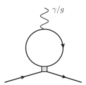
Figure 2: Diagram topology that cancels the residual scheme dependence in $a^{\gamma/g}$. The box denotes an insertion of a four-fermion operator.

Let us first consider the effect of the zero-mode Higgs only. We can partially use the results of [30] for the leptonic dimension-six dipole operator to construct the corresponding result in the quark sector. Again we only need to replace U(1) charges and add SU(3) colour factors as appropriate. For diagrams where a Higgs is emitted from an external leg and not from the loop (see the diagram in figure 3 for an example), one further has to distinguish two different contributions: those where the external quark propagator propagates KK modes and so-called off-shell terms that arise if the external propagator is a mass-less zero-mode, but the $1/p^{2}$ pole in the propagator is cancelled by powers of $p$ in the numerator, see [31] for a detailed discussion. The latter terms are basically irrelevant for leptons as they are effectively suppressed by a SM lepton Yukawa coupling. They may however play a role in the quark sector due to the large top Yukawa coupling and we include these terms in $a^{g/\gamma}$.

It is convenient to use the definition $D_{\mu}=\partial_{\mu}+iQ_{f}eA_{\mu}+ig_{s}T^{A}G_{\mu}$ for the SM covariant derivative with $A_{\mu}$, $G_{\mu}$ being photon and gluon field; $e$ is the charge of the positron. This definition then coincides with the choice usually employed in studies of the $b\to s\gamma$ transition, see e.g. [46, 55], and makes the expressions in the subsequent sections consistent with the standard literature.

In the minmal RS model we then find

$$\left.a_{ij}^{\gamma}\right|_{Higgs}= -\frac{e}{192\pi^{2}}\frac{T^{3}}{k^{4}}\,\frac{T^{8}}{2k^{8}}\left((2Q_{e}-Q_{d}-Q_{u})F_{Q}-Q_{d}F_{d}+(2Q_{e}-Q_{u})F_{u}\right)$$

$$-\frac{e}{192\pi^{2}}\frac{T^{3}}{k^{4}}\,\left(2Q_{d}+Q_{u}-Q_{e}\right)\,f^{(0)}_{Q_{i}}(1/T)[Y_{d}Y^{\dagger}_{d}Y_{d}]_{ij}\,g^{(0)}_{d_{j}}(1/T)$$ (13)

$$\left.a_{ij}^{g}\right|_{Higgs}= \phantom{-}\frac{g_{s}}{192\pi^{2}}\frac{T^{3}}{k^{4}}\,\frac{T^{8}}{2k^{8}}\left(2F_{Q}+F_{d}+F_{u}\right)$$

$$-\frac{g_{s}}{192\pi^{2}}\frac{T^{3}}{k^{4}}\,3\,f^{(0)}_{Q_{i}}(1/T)[Y_{d}Y^{\dagger}_{d}Y_{d}]_{ij}\,g^{(0)}_{d_{j}}(1/T)\,,$$ (14)

where the $F_{q}$ are abbreviations for

$$F_{d}= \hphantom{+}f^{(0)}_{Q_{i}}(1/T)[Y_{d}]_{ik}F(-c_{{d}_{k}})[Y^{\dagger}_{d}]_{kh}f^{(0)}_{Q_{h}}(1/T)^{2}[Y_{d}]_{hj}g^{(0)}_{d_{j}}(1/T)$$

$$F_{Q}= \hphantom{+}f^{(0)}_{Q_{i}}(1/T)[Y_{d}]_{ik}g^{(0)}_{d_{k}}(1/T)^{2}[Y^{\dagger}_{d}]_{kh}F(c_{{Q}_{h}})[Y_{d}]_{hj}g^{(0)}_{d_{j}}(1/T)$$

$$F_{u}= \hphantom{+}f^{(0)}_{Q_{i}}(1/T)[Y_{i}]_{ik}F(-c_{{u}_{k}})[Y^{\dagger}_{u}]_{kh}f^{(0)}_{Q_{h}}(1/T)^{2}[Y_{d}]_{hj}g^{(0)}_{d_{j}}(1/T)$$

$$F_{T_{3}}= \hphantom{+}f^{(0)}_{Q_{i}}(1/T)[Y_{d}]_{ik}F_{T_{3}}(c_{{d}_{k}})[Y^{\dagger}_{d}]_{kh}f^{(0)}_{Q_{h}}(1/T)^{2}Y_{hj}^{d}g^{(0)}_{d_{j}}(1/T),$$ (15)

with

$$F(c)\approx -\frac{k^{4}}{T^{5}}\,\frac{(3-2c)+(1+2c)\epsilon^{4c-2}-(3-2c)(1+2c)\epsilon^{2c-1}-(1-2c)^{2}\epsilon^{1+2c}}{(1+2c)(3-2c)(1-\epsilon^{2c-1})^{2}}\,,$$

$$F_{T_{3}}(c)\approx -\frac{k^{4}}{T^{5}}\,\frac{1-\epsilon^{1-2c}}{1-2c}\;.$$ (16)

In writing the expression for $F_{T_{3}}(c)$ we assume that the mass parameter $c$ is not too far from $-0.5$, which is realised for all parameter points that reproduce the low energy parameters of the SM.

In the custodially protected model the Higgs contribution to the dipole is given by

$$\left.a_{ij}^{\gamma}\right|_{Higgs}= -\frac{e}{192\pi^{2}}\frac{T^{3}}{k^{4}}\,\frac{T^{8}}{2k^{8}}\left((2Q_{e}-Q_{d}-Q_{u})(F_{Q}+F_{T_{3}})-Q_{d}F_{d}+(2Q_{e}-Q_{u})F_{u}\right)$$

$$-\frac{e}{192\pi^{2}}\frac{T^{3}}{k^{4}}\,\left(4Q_{d}+2Q_{u}-2Q_{e}\right)\,f^{(0)}_{Q_{i}}(1/T)[Y_{d}Y^{\dagger}_{d}Y_{d}]_{ij}\,g^{(0)}_{d_{j}}(1/T)$$ (17)

$$\left.a_{ij}^{g}\right|_{Higgs}= \phantom{-}\frac{g_{s}}{192\pi^{2}}\frac{T^{3}}{k^{4}}\,\frac{T^{8}}{2k^{8}}\left(2F_{Q}+2F_{T_{3}}+F_{d}+F_{u}\right)$$

$$-\frac{g_{s}}{192\pi^{2}}\frac{T^{3}}{k^{4}}\,6\,f^{(0)}_{Q_{i}}(1/T)[Y_{d}Y^{\dagger}_{d}Y_{d}]_{ij}\,g^{(0)}_{d_{j}}(1/T)\,.$$ (18)

The terms in (2.2.1), (2.2.1), (2.2.1) and (2.2.1) with factors of $F_{q}$, $q=T_{3},Q,u,d$, correspond to the off-shell contributions.

As already mentioned we also need to take into account the effect of Higgs KK modes. In [30] we absorbed the effect of the KK bosons in global factors called $R_{i}$. These were assumed to be roughly independent of the 5D mass parameters and therefore allowed for compact analytic expressions. Nevertheless there is a nontrivial dependence of the KK contribution on the 5D mass parameters; in particular for diagrams with a Higgs emission from an external line. In the lepton sector this effect is quite small especially when compared to the sizeable numerical uncertainties; we therefore neglected it in [30]. In the quark sector the wide range of 5D masses leads to more noticeable effects; since we can only determine these numerically we do not give an explicit expression. To give an idea of the potential size: the left panel in figure 3 shows the additional effect of the mass dependence (without numerical uncertainties) for the diagram shown on the right of the same figure. One can see that the effect is indeed of the order a few percent for leptons, but can potentially be of $\mathcal{O}(1)$ for quarks. It is therefore not feasible to use a simple analytic approximation as was done in the lepton sector.

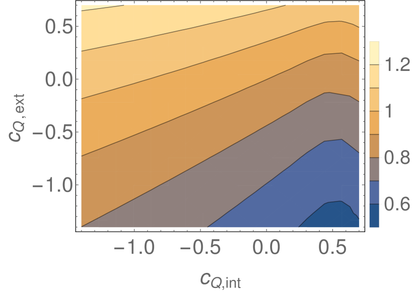
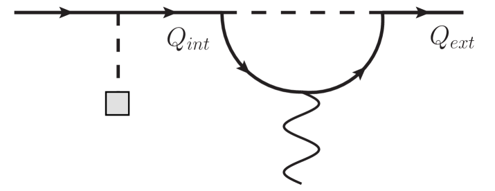
Figure 3: Illustration the additional dependence of the 5D mass parameter dependence of the KK Higgs contribution for the diagram on the right. $c_{Q_{int}},c_{Q_{ext}}$ are the 5D masses of the internal doublet propagator and the external doublet zero-mode. For leptons generally only a small region in the upper right corner ($c_{Q}\sim 0.4-0.7$) would be required.

.

Furthermore, we need to include KK Higgs corrections to the off-shell contributions to the Wilson coefficients. Again these terms are not necessarily suppressed in the quark sector, as the third generation Yukawa couplings are sizeable. However, we can only determine this contribution analytically for the Higgs zero-mode and not for the Higgs KK modes; it is only accessible numerically, but is quite small, only about $25\%$ of the corresponding zero-mode effect.

We therefore treat the effect of whole Higgs KK modes similarly to how the gauge-contribution is handled. Here we only remark that the total effect of the KK modes is smaller than the effect of the Higgs zero-mode but not parametrically so, see also [40, 30].

2.3 Beyond QCD

We only considered contributions to the Wilson coefficients that proportional to $\alpha_{s}$ or, in the case of dipole operators, enhanced by 5D Yukawa couplings. Obviously, exchange of hypercharge bosons and SU(2) bosons will also generate four-fermion operators, contribute to both dipoles and give rise to operators of the schematic form $\Phi^{\dagger}D_{\mu}\Phi\;\bar{q}\gamma^{\mu}q$. The latter class of operators will contribute to e.g. flavour-changing Z couplings.

The U(1) gauge coupling at a scale of $1\;\rm TeV$ is roughly $\alpha_{U(1)}\sim 0.01$. The SU(2)_L coupling is significantly larger with $\alpha_{SU(2)}(\mu=1\;\rm TeV)\sim 0.032$, but still smaller than $\alpha_{s}(\mu=1\;\rm TeV)=0.09$. The fact that the weak coupling is only about a factor of three smaller than the strong coupling may warrant including weak effects in the matching calculation. Including the effect of the other gauge bosons is not a principle problem; their contribution to the four-fermion coefficients as well as the dipole coefficients can directly be obtained from results for leptonic dipoles in the literature, see [30].

A further effect that would have be taken into account when considering weak corrections is the modification of of SM parameters and relations that have been utilised in the SM computation. In particular the relation of $G_{F}$ and the $W$ mass, that is frequently used when rewriting the SM expressions is affected by higher-dimensional operators (see [53] for the general case and [54] for the a discussion within the RS model).

It should be noted that KK Higgses do not give rise to relevant contributions to the four-fermion operators if the Higgs zero-mode is strongly localised towards the IR brane, which we always assume. An exchange of a SM Higgs can give a contribution to the four-fermion operators. But only in a second matching step at the intermediate scale $\mu_{int}\sim M_{W}$ when the Higgs degrees of freedom would be removed. In this case the flavour-changing Higgs coupling arise from dimension-six operators of the form $\bar{Q}_{i}\Phi D_{j}\;\Phi^{\dagger}\Phi$ (see e.g. [43]). However, even then the contribution will be suppressed by an additional SM b-quark Yukawa coupling. We therefore ignore these contributions.

3 Running to the low scale

The typical energy release in a decay of the type $\bar{B}\to X_{s}\gamma$ is of the order of the $b$ quark mass and a typical scale choice is thus $\mu_{b}\ =M_{B}/2\approx 2.6\,{\rm{GeV}}$. From the Standard Model calculation of $b\to s\gamma$ in the framework of the weak effective Hamiltonian, see [55] for an overview, it is known that the RGE evolution from the weak scale $\mu_{W}\sim M_{W}$ down to $\mu_{b}$ introduces sizeable operator mixing [56, 57].

Our matching calculation was performed the scale $\mu_{KK}\sim T$ and QCD corrections are bound to be of importance. We then have two possible strategies: We can either evolve the terms in the dimension-six Lagrangian from the high scale $\mu_{KK}$ to the electroweak scale within the unbroken SM, then change to the broken phase and complete the evolution down to the scale $\mu_{b}$. The required anomalous dimensions for the first step can be found e.g. in [53, 58, 59]. Alternatively, we can work with the “broken” operator basis already at the high scale and perform the evolution down to the low scale in one step (taking into account the top-mass threshold). The first approach is more in the spirit of a matching onto a set of dimension-six operators. The second option has simpler “logistics” as we only need consider a single RGE. Both strategies are valid and ultimately must be equivalent in a situation where no additional dynamics between $\mu_{KK}$ and $\mu_{W}$ need to be taken into account.

However, for the specific process at hand the second option has the additional advantage that the structure of the required evolution equation has been studied in some detail in [63]. While [63] ultimately focusses on scenarios with e.g. a flavour-changing $Z^{\prime}$, their operator basis contains the full set of normal and colour-flipped four-quark operators. We therefore choose to follow this approach.

Let us for clarity introduce the effective Hamiltonian at the high scale $\mu_{KK}$, that is used in [63]

$$\mathcal{H}^{(b\to s)}=-\frac{4G_{F}}{\sqrt{2}} V^{\star}_{ts}V_{tb}\bigg{[}\Delta C_{7\gamma}(\mu_{KK})Q_{7\gamma}+\Delta C_{8g}(\mu_{KK})Q_{8g}+\Delta C^{\prime}_{7\gamma}(\mu_{KK})Q^{\prime}_{7\gamma}+\Delta C^{\prime}_{8g}(\mu_{KK})Q^{\prime}_{8g}$$

$$+\sum_{A,B=L,R}\sum_{q=u,c,t,d,s,b}\Delta C^{q}_{1}[A,B](\mu_{KK})\,Q^{q}_{1}[A,B]+\Delta C^{q}_{2}[A,B](\mu_{KK})\;Q^{q}_{2}[A,B]$$

$$+\sum_{A,B=L,R}\Delta\widehat{C}^{d}_{1}[A,B](\mu_{KK})\,\widehat{Q}^{d}_{1}[A,B]+\Delta\widehat{C}^{d}_{2}[A,B](\mu_{KK})\;\widehat{Q}^{d}_{2}[A,B]\bigg{]}$$ (19)

where the operators are given by

$$Q_{7\gamma} =\frac{e\,m_{b}}{16\pi^{2}}\bar{s}_{\alpha}\sigma^{\mu\nu}P_{R}b_{\alpha}F_{\mu\nu} Q_{8g} =\frac{g_{s}\,m_{b}}{16\pi^{2}}\bar{s}_{\alpha}\sigma^{\mu\nu}P_{R}T^{A}_{\alpha\beta}b_{\beta}G^{A}_{\mu\nu}$$

$$Q^{\prime}_{7\gamma} =\frac{e\,m_{b}}{16\pi^{2}}\bar{s}_{\alpha}\sigma^{\mu\nu}P_{L}b_{\alpha}F_{\mu\nu} Q^{\prime}_{8g} =\frac{g_{s}\,m_{b}}{16\pi^{2}}\bar{s}_{\alpha}\sigma^{\mu\nu}P_{L}T^{A}_{\alpha\beta}b_{\beta}G^{A}_{\mu\nu}$$

$$Q^{q}_{1}[A,B] =(\bar{s}_{\alpha}\gamma^{\mu}P_{A}b_{\beta})\;(\bar{q}_{\beta}\gamma_{\mu}P_{B}q_{\alpha}) Q^{q}_{2}[A,B] =(\bar{s}_{\alpha}\gamma^{\mu}P_{A}b_{\alpha})\;(\bar{q}_{\alpha}\gamma_{\mu}P_{B}q_{\alpha})$$

$$\widehat{Q}^{d}_{1}[A,B] =(\bar{s}_{\alpha}\gamma^{\mu}P_{A}d_{\beta})\;(\bar{d}_{\beta}\gamma_{\mu}P_{B}b_{\alpha}) \widehat{Q}^{d}_{2}[A,B] =(\bar{s}_{\alpha}\gamma^{\mu}P_{A}d_{\alpha})\;(\bar{d}_{\alpha}\gamma_{\mu}P_{B}b_{\alpha})$$ (20)

with $P_{L/R}=\frac{1}{2}(1\mp\gamma_{5})$ as usual and $\alpha,\,\beta$ are colour indices. Note that while the usual current-current and penguin operators

$$Q_{1} =(\bar{s}_{\alpha}\gamma^{\mu}P_{L}c_{\beta})\;(\bar{c}_{\beta}\gamma_{\mu}P_{L}b_{\alpha}) Q_{2} =(\bar{s}_{\alpha}\gamma^{\mu}P_{L}c_{\alpha})\;(\bar{c}_{\beta}\gamma_{\mu}P_{L}b_{\beta})$$

$$Q_{3} =(\bar{s}_{\alpha}\gamma^{\mu}P_{L}c_{\alpha})\!\!\!\sum_{q=u,c,d,s,b}(\bar{q}_{\beta}\gamma_{\mu}P_{L}q_{\beta}) Q_{4} =(\bar{s}_{\alpha}\gamma^{\mu}P_{L}c_{\beta})\!\!\!\sum_{q=u,c,d,s,b}(\bar{q}_{\beta}\gamma_{\mu}P_{L}q_{\alpha})$$

$$Q_{5} =(\bar{s}_{\alpha}\gamma^{\mu}P_{L}c_{\alpha})\!\!\!\sum_{q=u,c,d,s,b}(\bar{q}_{\beta}\gamma_{\mu}P_{R}q_{\beta}) Q_{6} =(\bar{s}_{\alpha}\gamma^{\mu}P_{L}c_{\beta})\!\!\!\sum_{q=u,c,d,s,b}(\bar{q}_{\beta}\gamma_{\mu}P_{R}q_{\alpha})$$ (21)

are not included in (3), they do enter the renormalisation group equations. This operator basis is obviously non-minimal as e.g. $Q_{1}$ and $Q^{c}_{2}[L,L]$ are related via Fierz identities. As we only consider the LO corrections due to new physics, this does not invalidate the RG analysis [55].

In total we have to consider $70$ operators. Fortunately, there are only a few independent entries in the leading order (LO) anomalous dimension matrix. Most of which can be taken from [60, 61] once the different operator normalisation has been taken into account. The remaining entries can be taken directly from [63] where the use of effective, scheme-independent coefficients $C_{7\gamma}^{eff}$, $C_{8g}^{eff}$ is implied. In the following we tacitly assume that $C_{7/8}$ refers to the effective quantity and forgo to display the superscript. We will not give the anomalous dimensions explicitly and refer to the original literature for details.

With the anomalous dimensions at hand, the renormalisation group evolution equation (RGE)

$$\mu\frac{d}{d\mu}\vec{C}_{i}(\mu)=\frac{\alpha_{s}(\mu)}{4\pi}[\gamma^{T}]_{ij}\vec{C}_{j}(\mu)$$ (22)

can be solved in the standard way, provided the initial conditions at the high scale $\mu_{KK}$ are known. As the anomalous dimension matrix $\gamma$ is sparse, a basis where the evolution is diagonal can be determined very efficiently. For the strong coupling constant we use $\alpha_{s}(M_{Z})=0.1185$ with decoupling of the top quark at $m_{t}=170\,{\rm GeV}$.

Once the evolution down to $\mu_{b}$ has been performed the result for the branching fraction of $\bar{B}\to X_{s}\gamma$ can be obtained using the formula [63, 64]

$$\frac{\left.\text{Br}\left(B\to X_{s}\gamma\right)\right|_{E_{\gamma}>1.6\,{\rm GeV}}}{\left.\text{Br}\left(B\to X_{s}\gamma\right)\right|^{SM}_{E_{\gamma}>1.6\,{\rm GeV}}}=\frac{1}{\left|C_{7\gamma}(\mu_{b})^{SM}\right|^{2}+N}\left(\left|C_{7\gamma}(\mu_{b})\right|^{2}+\left|C^{\prime}_{7\gamma}(\mu_{b})\right|^{2}+N\right)\;.$$ (23)

Here we use a minimum photon energy of $E_{\gamma}^{min}=1.6\,{\rm GeV}$; the same as was used for the HFAG world average. Here the $N$ is a non-perturbative correction [65, 66, 67, 68] and we use $N(E_{\gamma}=1.6\;{\rm GeV})=3.6\times 10^{-3}$.

Since we work in leading order in the new physics contribution, BSM effects only induce a shift in the Wilson coefficients

$$C^{(\prime)}_{7\gamma}(\mu_{b})\to\left[C^{(\prime)}_{7\gamma}(\mu_{b})\right]_{SM}+\Delta C^{(\prime)}_{7\gamma}(\mu_{b})\;.$$ (24)

The SM value of the dipole coefficients

$$C_{7\gamma}(\mu_{b})=-0.368$$ (25)

can be taken from [15]. The primed coefficient $C_{7\gamma}$ is tiny as it is suppressed by $m_{s}/m_{b}$ and can be neglected.

For completeness we also give the formulae for the related process $b\to sg$. It can be treated completely analogously; here the shifts in the coefficients $C^{(\prime)}_{8g}(\mu_{b})$ are required. The NLL SM prediction was determined in [69]. The partial width for the process $b\to sg$ is given by

$$\Gamma\left(\bar{B}\to sg\right)=\frac{\alpha_{s}(m_{b})m_{b}^{5}}{24\pi^{2}}\left|G_{F}V_{ts}^{\star}V_{tb}\right|^{2}|D|^{2}+\Gamma_{fin}^{\text{brems}}\;.$$ (26)

The explicit expressions for $\Gamma_{fin}^{\text{brems}}$ and $D$ can be found in [69]. The branching fraction is then obtained as

$${\text{Br}}(b\to sg)\approx\frac{\Gamma(b\to sg)}{\Gamma(b\to ce\bar{\nu}_{e})}\mathcal{B}^{exp}_{sl}\;.$$ (27)

With $\mathcal{B}^{exp}_{sl}\approx 0.105\pm 0.005$ being the experimental semi-leptonic branching fraction of the B-meson. In the SM one finds [69]

$${\text{Br}}^{SM}(b\to sg)=(5.0\pm 1.0)\times 10^{-3}\;.$$ (28)

The last missing piece for our analysis are the initial conditions for the RGE. That is, we need the Wilson coefficients $\Delta C$ in (3).

Initial conditions

The Wilson coefficient in $\mathcal{H}^{b\to s}$ at the high scale $\mu_{KK}$ can be obtained from the Wilson coefficients of the dimension-six operators in (2). We need to rotate into the low-energy mass basis and replace the SM Higgs field (if present) by its vacuum expectation value $v/\sqrt{2}$:

$$\Phi\to\begin{pmatrix}\phi^{+}\\ \frac{1}{\sqrt{2}}(v+h+iG)\end{pmatrix} Q_{i}\to P_{L}\begin{pmatrix}U^{u}_{ij}u_{j}\\ U^{d}_{ij}d_{j}\end{pmatrix} U_{i}\to V^{u}_{ij}P_{R}u_{j} D_{i}\to V^{d}_{ij}P_{R}d_{j}\;.$$ (29)

We only take into account terms that contribute to the Wilson coefficients in (3) and drop all others.

As an example, let us consider the term $b^{DU}_{ij}\bar{D}_{i}\gamma^{\mu}T^{a}D_{i}\bar{U}_{j}\gamma^{\mu}T^{a}U_{j}$ in the dimension-six Lagrangian. Using the substitution rules (29) we find

$$b^{DU}_{ij}\bar{D}_{i} \gamma^{\mu}T^{A}D_{i}\bar{U}_{j}\gamma_{\mu}T^{A}U_{j}\longrightarrow\beta^{DU}_{sbq_{u}q_{u}}\,\bar{s}\gamma^{\mu}T^{A}P_{R}b\,\bar{q}_{u}\gamma_{\mu}T^{A}P_{R}q_{u}\,=$$

$$=-\frac{1}{2N_{c}}\beta^{DU}_{sbq_{u}q_{u}}\,\bar{s}\gamma^{\mu}P_{R}b\,\bar{q}_{u}\gamma_{\mu}P_{R}q_{u}+\frac{1}{2}\beta^{DU}_{sbq_{u}q_{u}}\,\bar{s}_{\alpha}\gamma^{\mu}P_{R}b_{\beta}\,(\bar{q}_{u})_{\beta}\gamma_{\mu}P_{R}(q_{u})_{\alpha}$$

$$=-\frac{1}{2N_{c}}\beta^{DU}_{sbq_{u}q_{u}}\,O_{2}^{q_{u}}[R,R]+\frac{1}{2}\beta^{DU}_{sbq_{u}q_{u}}\,O_{1}^{q_{u}}[R,R]$$ (30)

where a simple single sum over $q_{u}=u,c,t$ is implied. Here we defined $\beta^{DU}_{sbq_{u}q_{u}}=[V^{d}]^{\dagger}_{si}[V^{u}]^{\dagger}_{q_{u}j}b^{DU}_{ij}V^{d}_{ib}V^{u}_{jq_{u}}$. In general we will use the abbreviation

$$\beta^{FF^{\prime}}_{ABCD}=[R^{F}]^{\dagger}_{Ai}[R^{F^{\prime}}]^{\dagger}_{Cj}b^{FF^{\prime}}_{ij}R^{F}_{iB}R^{F^{\prime}}_{jD}$$ (31)

with the appropriate flavour rotation matrices $R^{F^{(\prime)}}$.

Comparing (3) with (3), we obtain

$$\frac{4G_{F}V^{\star}_{ts}V_{tb}}{\sqrt{2}}\Delta C^{q_{u}}_{1}[R,R](\mu_{KK})=\frac{1}{2T^{2}}\beta^{DU}_{sbq_{u}q_{u}}, \frac{4G_{F}V^{\star}_{ts}V_{tb}}{\sqrt{2}}\Delta C^{q_{u}}_{2}[R,R](\mu_{KK})=-\frac{1}{2N_{c}T^{2}}\beta^{DU}_{sbq_{u}q_{u}}\,.$$ (32)

The remaining four-quark operators can be related to operators in the weak Hamiltonian in the same fashion. For clarity, we have relayed the expressions for the Wilson coefficient of (3) to an Appendix.

Similarly, we can obtain the effective dipole operator coefficients. Introducing the abbreviation $\alpha^{\gamma/g}=U_{d}^{\dagger}a^{\gamma/g}V_{d}$ we find

$$\frac{4G_{F}V^{\star}_{ts}V_{tb}}{\sqrt{2}}C_{7\gamma}(\mu_{KK}) =\frac{16\pi^{2}}{e\,m_{b}\,T^{2}}\phantom{[}\alpha^{\gamma}_{sb}\phantom{]^{\dagger}}\frac{v}{\sqrt{2}}+\sum_{q=d,s,b}\frac{Q_{q}\,m_{q}\,C_{F}}{m_{b}\,T^{2}}\beta^{QD}_{qbsq}$$

$$\frac{4G_{F}V^{\star}_{ts}V_{tb}}{\sqrt{2}}C^{\prime}_{7\gamma}(\mu_{KK}) =\frac{16\pi^{2}}{e\,m_{b}\,T^{2}}[\alpha^{\gamma}]^{\dagger}_{sb}\frac{v}{\sqrt{2}}+\sum_{q=d,s,b}\frac{Q_{q}\,m_{q}\,C_{F}}{m_{b}\,T^{2}}\beta^{QD}_{sqqb}$$

$$\frac{4G_{F}V^{\star}_{ts}V_{tb}}{\sqrt{2}}C_{8g}(\mu_{KK}) =\frac{16\pi^{2}}{g_{s}\,m_{b}\,T^{2}}\phantom{[}\alpha^{g}_{sb}\phantom{]^{\dagger}}\frac{v}{\sqrt{2}}-\sum_{q=d,s,b}\frac{m_{q}}{2N_{c}\,m_{b}\,T^{2}}\beta^{QD}_{qbsq}$$

$$\frac{4G_{F}V^{\star}_{ts}V_{tb}}{\sqrt{2}}C^{\prime}_{8g}(\mu_{KK}) =\frac{16\pi^{2}}{g_{s}\,m_{b}\,T^{2}}[\alpha^{g}]^{\dagger}_{sb}\frac{v}{\sqrt{2}}-\sum_{q=d,s,b}\frac{m_{q}}{2N_{c}\,m_{b}\,T^{2}}\beta^{QD}_{sqqb}\;.$$ (33)

All quantities on the right-hand side of (33) are implied to be evaluated at the scale $\mu_{KK}$. The terms containing a $\beta$-coefficient arise from the one-loop diagrams with an insertion of a four-fermion operator. They ensure that the (effective) coefficient $\Delta C_{7\gamma}$ is scheme independent, see Sec. 2.2.

4 Phenomenology

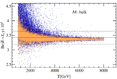
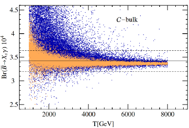
Figure 4: ${\rm{Br}}(\overline{B}\to X_{s}\gamma)$ as a function of the KK scale $T$. The blue (dark grey) points correspond to the data set with large Yukawas, $Y_{max}=3$. The orange (light grey) points correspond to $Y_{max}=1/2$. The horizontal lines indicate the experimental value of and uncertainty on the branching fraction. The left panel shows the result for the minimal RS model, the right panel for the custodially protected model.

To see the potential effect of the additional contribution to $C_{7\gamma}^{(\prime)}$ on the $B\to X_{s}\gamma$ decay we need to scan over the parameter space of the RS model. We will, as mentioned before, consider a minimal and a custodially protected RS model with an IR-localised bulk Higgs. The model parameters include the 5D masses of the fermions as well as the two Yukawa couplings $Y_{d}$ and $Y_{u}$. These parameters are not independent as we need to impose the condition that low-energy parameters of the SM are reproduced within uncertainties. We take into account the SM quark masses (at the scale $T$) and the CKM angles and phase; here we make use of the analytic approximations of [25]. A further restriction is imposed by hand on the dimensionless Yukawa matrices as we require them to be anarchic. That is, the matrix elements all have roughly a common magnitude of $\mathcal{O}(1)$ and arbitrary phase. Similar to the analysis in [30] we consider two samples of Yukawas: one with a maximum entry size of $Y_{max}=3$ (representing the case of large Yukawa couplings) and one with an upper bound of $Y_{max}=1/2$ (representing the case of small Yukawa couplings).

The main result of our scan through the RS parameter space is shown in figure 4. It shows the branching fraction $\bar{B}\to X_{s}\gamma$ as a function of the KK scale $T$ for the minimal RS model (left panel) and the custodially protected model (right panel). The blue (dark grey) points correspond to $Y_{max}=3$, the orange (light grey) points to $Y_{max}=1/2$. The current experimental central value, see equation (1), is represented by the solid horizontal line; the dashed lines indicate the uncertainty.

We find that the branching fraction is, especially for small Yukawas, predominantly larger than in the SM. This is due to a sizeable contribution from $C_{7\gamma}^{\prime}$, that lacks an unsuppressed interference term with the SM contribution—its contribution to the branching fraction is always positive. In addition to that the contribution to $C_{7\gamma}^{\prime}$ is generally larger than the contribution to the unprimed dipole coefficient. The reason for this, as was observed already in [41], is that the 5D profile of the doublet $Q_{3}$ (that very roughly corresponds to the $b_{L}$ after EWSB) is typically larger than the profiles of the down-type singlets $D$ near the IR brane; consequently the operator $Q_{7,\gamma}^{\prime}\propto(\overline{s_{R}})_{\alpha}\sigma^{\mu\nu}(b_{L})_{\alpha}F_{\mu\nu}$ receives a larger BSM contribution.

Only for the $Y_{max}=3$ sample one can observe data points with a significantly reduced branching fraction compared to the SM. This is due to a destructive interference of $C_{7\gamma}^{SM}$ and $\Delta C_{7\gamma}$ that can counteract the contribution due to $C_{7\gamma}^{\prime}$ if the Higgs contribution to $C_{7,\gamma}(\mu_{KK})$ is large. This effect is more pronounced in the custodially protected model where the additional fermion states enhance the dipole coefficient, cp. (2.2.1) and (2.2.1). For small Yukawas the phenomenology of minimal and custodially protected model is quite similar. This is to some extent a consequence of working only with QCD- and Higgs-mediated contributions to the Wilson coefficient; QCD is treated the same in both models while the electroweak sector is extended and features additional bosonic modes. In the $Y_{max}=1/2$ scenario the main distinction between the two models—the Higgs contribution— is suppressed.

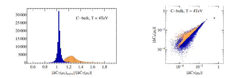
Figure 5: left panel: Effect of operator mixing on $\Delta C_{7\gamma}$. The histogram shows the distribution of $|\Delta C_{7\gamma}(\mu_{b})|$ without operator mixing relative to the full $|\Delta C_{7\gamma}(\mu_{b})|$ with mixing (see text for details). The blue (dark grey) and orange (light grey) histogram corresponds to $Y_{max}=3$ and $Y_{max}=1/2$. right panel: Correlation of $\Delta C_{8g}$ and $\Delta C_{7\gamma}$ in the custodially protected RS model for $T=4\,{\rm TeV}$. The triangle represents the SM values of $C_{7\gamma}$ and $C_{8g}$; the dashed diagonal line indicates $|\Delta C_{8g}|=|\Delta C_{7\gamma}|$. Same colour coding as in the left panel.

The smallness of the Higgs contribution for $Y_{max}=1/2$ and the consequently smaller $\Delta C_{7\gamma}(\mu_{KK})$ also make the inclusion of operator mixing mandatory. To see this we consider two quantities: the full $\Delta C_{7\gamma}(\mu_{b})$ as obtained from the RGE (22) and $\Delta C_{7\gamma}(\mu_{b})|_{naive}$ which is also obtained via (22) but we set the Wilson coefficients of all four-fermion operators at the high scale $\mu_{KK}$ to zero. We then consider the ratio $\Delta C_{7\gamma}(\mu_{b})|_{naive}/\Delta C_{7\gamma}(\mu_{b})$. The deviation of the ratio from one indicates the relative importance of the four-fermion operators for the $b\to s\gamma$ transition. Histograms of $\Delta C_{7\gamma}(\mu_{b})|_{naive}/\Delta C_{7\gamma}(\mu_{b})$ are shown in the left panel of figure 5. For simplicity we only show the plot in the minimal model for $T=4\,{\rm TeV}$. For large Yukawas, $Y_{max}=3$ in blue (dark grey), neglecting the contribution of from four-fermion operators leads on average to an increase of $\Delta C_{7\gamma}(\mu_{b})$ by $5\%$. For a few Yukawa data sets the shift can be of the order of $\pm 15\%$. In the case of small 5D Yukawa coupling (shown in orange) ignoring the four-fermion operator mixing basically always increases $\Delta C_{7}$. This can lead to an overestimate of the BSM contribution to the $\bar{B}\to X_{s}\gamma$ branching fraction by up to $40\%$. Hence including the mixing is relevant and should not be neglected. This is of course quite general as FCNCs mediated by new, massive gauge bosons usually create simultaneous contributions to $\Delta C_{7\gamma}$ and to the $\Delta C_{1,2}^{q}[A,B]$ as is indicated by the need to include the four-fermion operators to obtain a scheme-independent result.

For completeness we also show the correlation of $\Delta C_{7\gamma}(\mu_{b})$ and $\Delta C_{8\gamma}(\mu_{b})$ in the right panel of figure 5. We see that on average the BSM contribution to $C_{7\gamma}$ is smaller than the contribution to $C_{8g}$ as was also noted in [24]. This is more noticeable for the small Yukawa sample shown in orange (light grey). The two Wilson coefficients are then clearly correlated and one observes a ”lower bound” on $\Delta C_{7\gamma}$ for a given value of $\Delta C_{8\gamma}$. However, with $Y_{max}=3$, it is straightforward to find parameter points where $\Delta C_{7\gamma}$ is much larger than the BSM contribution to $C_{8g}$. The reason for this is the following: The zero-mode Higgs contribution to $a^{g}$ and $a^{\gamma}$ are almost proportional to each other, see equations (2.2.1)–(2.2.1). However, the sizeable KK Higgs contribution has a more complicated structure; it contributes in a different way to $a^{g}$ and to $a^{\gamma}$. This blurs the correlation.

Finally, comparing with the experimental value for $\bar{B}\to X_{s}\gamma$ we find that for $Y_{max}=1/2$ the RS model parameter space is generally compatible with experimental data for $T>2\;{\rm TeV}$. Since electroweak precision observables already put stricter bounds on the KK scale [25, 26], $\bar{B}\to X_{s}\gamma$ does not give any new constraints on the KK scale. Nonetheless, sizeable corrections of about $5-10\%$ are still possible. For large Yukawas the situation is much more intriguing, especially in the custodially protected model. As the large effects come almost exclusively from the Higgs exchange contribution to the dipole coefficients $a^{g/\gamma}$ they are strongly dependent on the specific form of the anarchic Yukawa matrices. It is difficult to deduce any hard bounds on the RS parameter space. However, the total BSM correction to the branching fraction can be quite substantial. Even for $T\sim 5\;{\rm TeV}$ it is easy to find parameter points outside the current experimental limits. Consequently, the new Belle II searches would have the potential to discover the impact of KK states on $\bar{B}\to X_{s}\gamma$ with masses well above $10\;{\rm TeV}$. The search at the B-factory is therefore complementary to other powerful indirect search avenues like Higgs production and decay or dipole moments — experiments at vastly different energy scales.

5 Conclusion

We have studied the flavour violating radiative transition $b\to s\gamma$ in RS models with an IR localised bulk Higgs. For simplicity, our analysis is restricted to QCD- and Higgs-mediated BSM effects. We followed the strategy of [31] and matched the five-dimensional RS model onto the SM effective theory including dimension-six operators. Here we could make use of our recent results [30] for lepton-flavour violation in the RS model. In particular the complicated 5D loop integrals that determine the dimension-six quark dipole coefficients could be recovered from the electromagnetic dipole coefficient for leptons. This way we can include the effect of 5D loops with internal gauge, Higgs as well as KK Higgs bosons.

After the transition to the broken electroweak phase, we used the results of [63] to include the effect of operator mixing due to RGE evolution from the KK scale $T$ to $\mu_{b}$ to LL accuracy. This is necessary as already in the SM the QCD corrections are sizeable and the dipole operator coefficient alone is not regularisation scheme independent. We find that for small Yukawa couplings, i.e., for small Higgs contributions to the dimension-six dipoles, the mixing of additional four-fermion Wilson coefficients into $C_{7,8}$ can be sizeable and should not be neglected. We expect this to be true in any BSM model where dipole and four-fermion operators are generated via exchange of the same intermediate states.

While our results for the Wilson coefficients are general, we assumed anarchic Yukawa couplings to study the phenomenology of the decay $\bar{B}\to X_{s}\gamma$ in both the minimal and the custodially protected RS model. We find that the additional contributions to the branching fraction can be sizeable for large Yukawas and moderate KK scales $T$.

The strong sensitivity of the RS contribution to the specific form of the Yukawa matrices makes it challenging to directly constrain the parameter space of the model. Nonetheless, the decay is a useful tool that complements other powerful probes for the KK scale in the quark sector, like Higgs production/decay [35, 38, 37]. More importantly, for large 5D quark Yukawas there can be observable deviations of ${\rm Br}(\bar{B}\to X_{s}\gamma)$ from its SM value even for masses of the first KK excitation of around $10\;{\rm TeV}$. For small 5D Yukawas couplings ($Y_{max}\sim 0.5$) the impact of the RS model is mild; for KK scales that are not in conflict with electroweak precision measurements the $\bar{B}\to X_{s}\gamma$ branching fraction generally agrees with the current world average within uncertainties. In this case the aforementioned alternative search channels are more promising.

Note added:

While this work was in its final stage, [71] was published. [71] presents a detailed analysis of the $b\to s\gamma$ transition in the minimal RS model with an exactly brane-localised Higgs. It is to our knowledge also the first computation of the RS contribution to dipole operators that does not rely on an expansion in the ratio of electroweak and KK scale. In addition to QCD and Higgs effects also electroweak effects are taken into account, but the model does, by construction, not involve Kaluza Klein Higgs contributions. [71] includes QCD operator mixing, but neglects the effect of the four-fermion operators. Since we consider the case of a localised bulk Higgs with KK modes, it is most useful to compare with the case of small Yukawa couplings; in this case the quite different Higgs sector does not play an all too dominant role. We then find RS corrections to ${\rm Br}(\bar{B}\to X_{s}\gamma)$ that are of similar but slightly smaller in size to those found [71]. This seems not unexpected as we neglect electroweak corrections to the dipole, but do include mixing with dimension-six fermion operators, which tends to give rise to a slightly smaller $\Delta C_{7\gamma}$ coefficient.

Acknowledgements:

We are grateful to M. Beneke for suggesting this project and for many useful discussions. The work of P.M. is supported in part by the Gottfried Wilhelm Leibniz programme of the Deutsche Forschungsgemeinschaft (DFG). The work of J.R. is supported by STFC UK. We thank the Munich Institute for Astro- and Particle Physics (MIAPP) of the DFG cluster of excellence “Origin and Structure of the Universe” for hospitality during part of the work. The Feynman diagrams were drawn with the help of Axodraw [72] and JaxoDraw [73].

Appendix A Wilson coefficients of the extended electroweak Hamiltonian at the scale $\mu_{KK}$

In the following we collect the coefficients of the various four-fermion operators in (3). To this end we first map each operator in the dimension-six Lagrangian unto operators in the broken electroweak theory and extract the Wilson coefficients by comparing with (3). For brevity, let us first introduce the abbreviation $\mathcal{V}=\frac{4G_{F}V^{\star}_{ts}V_{tb}}{\sqrt{2}}$.

$$b^{QU}_{ij}\bar{Q}_{i} \gamma^{\mu}T^{A}Q_{i}\bar{U}_{j}\gamma_{\mu}T^{A}U_{j}\longrightarrow\beta^{QU}_{sbq_{u}q_{u}}\,\bar{s}\gamma^{\mu}T^{A}P_{R}b\,\bar{q}_{u}\gamma_{\mu}T^{A}P_{R}q_{u}\,=$$

$$=-\frac{1}{2N_{c}}\beta_{sbq_{u}q_{u}}\,\bar{s}\gamma^{\mu}P_{L}b\,\bar{q}_{u}\gamma^{\mu}P_{R}q_{u}+\frac{1}{2}\beta_{sbuu}\,\bar{s}_{\alpha}\gamma^{\mu}P_{L}b_{\beta}\,(\bar{q}_{u})_{\beta}\gamma^{\mu}P_{R}(q_{u})_{\alpha}$$

$$=-\frac{1}{2N_{c}}\beta_{sbq_{u}q_{u}}\,O_{2}^{q_{u}}[L,R]+\frac{1}{2}\beta_{sbq_{u}q_{u}}\,O_{1}^{q_{u}}[L,R]$$ (34)

gives

$$\mathcal{V}\Delta C^{q_{u}}_{1}[L,R](\mu_{KK})=\frac{1}{2T^{2}}\beta^{QU}_{sbq_{u}q_{u}} \mathcal{V}\Delta C^{q_{u}}_{2}[L,R](\mu_{KK})=-\frac{1}{2N_{c}T^{2}}\beta^{QU}_{sbq_{u}q_{u}}\,.$$ (35)

$$b^{DD}_{ij}\bar{D}_{i} \gamma^{\mu}T^{A}D_{i}\bar{D}_{j}\gamma_{\mu}T^{A}D_{j}\longrightarrow$$

$$=-\frac{1}{N_{c}}\beta^{DD}_{sbdd}\,O_{2}^{d}[R,R]+\beta^{DD}_{sbdd}\,O_{1}^{d}[R,R]-\frac{1}{N_{c}}\beta^{DD}_{sddb}\,\widehat{O}_{2}^{d}[R,R]+\beta^{DD}_{sddb}\,\widehat{O}_{1}^{d}[R,R]$$ (36)

$$\phantom{=}-\frac{1}{N_{c}}\beta^{DD}_{sbbb}\,O_{2}^{b}[R,R]+\beta^{DD}_{sbbb}\,O_{1}^{b}[R,R]-\frac{1}{N_{c}}\beta^{DD}_{sbss}\,O_{2}^{s}[R,R]+\beta^{DD}_{sbss}\,O_{1}^{s}[R,R]$$ (37)

gives

$$\mathcal{V}\Delta C^{s}_{1}[R,R](\mu_{KK})=\frac{1}{T^{2}}\beta^{DD}_{sbss} \mathcal{V}\Delta C^{s}_{2}[R,R](\mu_{KK})=-\frac{1}{N_{c}T^{2}}\beta^{DD}_{sbss}$$

$$\mathcal{V}\Delta C^{b}_{1}[R,R](\mu_{KK})=\frac{1}{T^{2}}\beta^{DD}_{sbbb} \mathcal{V}\Delta C^{b}_{2}[R,R](\mu_{KK})=-\frac{1}{N_{c}T^{2}}\beta^{DD}_{sbbb}$$

$$\mathcal{V}\Delta C^{d}_{1}[R,R](\mu_{KK})=\frac{1}{T^{2}}\beta^{DD}_{sbdd} \mathcal{V}\Delta C^{d}_{2}[R,R](\mu_{KK})=-\frac{1}{N_{c}T^{2}}\beta^{DD}_{sbdd}$$

$$\mathcal{V}\Delta\widehat{C}^{d}_{1}[R,R](\mu_{KK})=\frac{1}{T^{2}}\beta^{DD}_{sddb} \mathcal{V}\Delta\widehat{C}^{d}_{2}[R,R](\mu_{KK})=-\frac{1}{N_{c}T^{2}}\beta^{DD}_{sddb}$$ (38)

$$b^{QQ}_{ij}\bar{Q}_{i} \gamma^{\mu}T^{A}Q_{i}\bar{Q}_{j}\gamma_{\mu}T^{A}Q_{j}\longrightarrow$$

$$=-\frac{1}{N_{c}}\beta^{QQ}_{sbuu}\,O_{2}^{u}[L,L]+\beta^{QQ}_{sbuu}\,O_{1}^{u}[L,L]$$

$$\phantom{=}-\frac{1}{N_{c}}\beta^{QQ}_{sbdd}\,O_{2}^{d}[L,L]+\beta^{QQ}_{sbbb}\,O_{1}^{d}[L,L]-\frac{1}{N_{c}}\beta^{QQ}_{sddb}\,\widehat{O}_{2}^{s}[L,L]+\beta^{QQ}_{sddb}\,\widehat{O}_{1}^{s}[L,L]$$

$$\phantom{=}-\frac{1}{N_{c}}\beta^{QQ}_{sbss}\,O_{2}^{d}[L,L]+\beta^{QQ}_{sbss}\,O_{1}^{s}[L,L]-\frac{1}{N_{c}}\beta^{QQ}_{sbbb}\,O_{2}^{b}[L,L]+\beta^{QQ}_{sbbb}\,O_{1}^{b}[L,L]$$ (39)

gives

$$\mathcal{V}\Delta C^{s}_{1}[L,L](\mu_{KK})=\frac{1}{T^{2}}\beta^{QQ}_{sbss} \mathcal{V}\Delta C^{s}_{2}[L,L](\mu_{KK})=-\frac{1}{N_{c}T^{2}}\beta^{QQ}_{sbss}$$

$$\mathcal{V}\Delta C^{b}_{1}[L,L](\mu_{KK})=\frac{1}{T^{2}}\beta^{QQ}_{sbbb} \mathcal{V}\Delta C^{b}_{2}[L,L](\mu_{KK})=-\frac{1}{N_{c}T^{2}}\beta^{QQ}_{sbbb}$$

$$\mathcal{V}\Delta C^{d}_{1}[L,L](\mu_{KK})=\frac{1}{T^{2}}\beta^{QQ}_{sbdd} \mathcal{V}\Delta C^{d}_{2}[L,L](\mu_{KK})=-\frac{1}{N_{c}T^{2}}\beta^{QQ}_{sbdd}$$

$$\mathcal{V}\Delta\widehat{C}^{d}_{1}[L,L](\mu_{KK})=\frac{1}{T^{2}}\beta^{QQ}_{sddb} \mathcal{V}\Delta\widehat{C}^{d}_{2}[L,L](\mu_{KK})=-\frac{1}{N_{c}T^{2}}\beta^{QQ}_{sddb}$$

$$\mathcal{V}\Delta{C}^{q_{u}}_{1}[L,L](\mu_{KK})=\frac{1}{T^{2}}\beta^{QQ}_{sdq_{u}q_{u}} \mathcal{V}\Delta{C}^{q_{u}}_{2}[L,L](\mu_{KK})=-\frac{1}{N_{c}T^{2}}\beta^{QQ}_{sbq_{u}q_{u}}$$ (40)

Finally

$$b^{QD}_{ij}\bar{Q}_{i} \gamma^{\mu}T^{A}Q_{i}\bar{D}_{j}\gamma_{\mu}T^{A}D_{j}\longrightarrow$$

$$=-\frac{1}{2N_{c}}\beta^{QD}_{uusb}\,O_{2}^{u}[R,L]+\frac{1}{2}\beta^{QD}_{uusb}\,O_{1}^{u}[R,L]$$

$$\phantom{=}-\frac{1}{2N_{c}}\beta^{QD}_{sbdd}\,O_{2}^{d}[L,R]+\frac{1}{2}\beta^{QD}_{sbdd}\,O_{1}^{d}[L,R]-\frac{1}{2N_{c}}\beta^{QD}_{ddsb}\,O_{2}^{d}[R,L]+\frac{1}{2}\beta^{QD}_{ddsb}\,O_{1}^{d}[R,L]$$

$$\phantom{=}-\frac{1}{2N_{c}}\beta^{QD}_{sddb}\,\widehat{O}_{2}^{d}[L,R]+\frac{1}{2}\beta^{QD}_{sddb}\,\widehat{O}_{1}^{d}[L,R]-\frac{1}{2N_{c}}\beta^{QD}_{dbsd}\,\widehat{O}_{2}^{d}[R,L]+\frac{1}{2}\beta^{QD}_{dbsd}\,\widehat{O}_{1}^{d}[R,L]$$

$$\phantom{=}-\frac{1}{2N_{c}}\beta^{QD}_{sbss}\,{O}_{2}^{s}[L,R]+\frac{1}{2}\beta^{QD}_{sbss}\,{O}_{1}^{s}[L,R]-\frac{1}{2N_{c}}\beta^{QD}_{sssb}\,{O}_{2}^{s}[R,L]+\frac{1}{2}\beta^{QD}_{sssb}\,{O}_{1}^{s}[R,L]$$

$$\phantom{=}-\frac{1}{2N_{c}}\beta^{QD}_{sbbb}\,{O}_{2}^{b}[L,R]+\frac{1}{2}\beta^{QD}_{sbbb}\,{O}_{1}^{b}[L,R]-\frac{1}{2N_{c}}\beta^{QD}_{bbsb}\,{O}_{2}^{b}s[R,L]+\frac{1}{2}\beta^{QD}_{bbsb}\,{O}_{1}^{b}[R,L]$$ (41)

gives

$$\mathcal{V}\Delta C^{q_{u}}_{1}[R,L](\mu_{KK})=\frac{1}{2T^{2}}\beta^{QD}_{q_{u}q_{u}sb} \mathcal{V}\Delta C^{q_{u}}_{2}[R,L](\mu_{KK})=-\frac{1}{2N_{c}T^{2}}\beta^{QD}_{q_{u}q_{u}sb}$$

$$\mathcal{V}\Delta C^{d}_{1}[R,L](\mu_{KK})=\frac{1}{2T^{2}}\beta^{QD}_{ddsb} \mathcal{V}\Delta C^{d}_{2}[R,L](\mu_{KK})=-\frac{1}{2N_{c}T^{2}}\beta^{QD}_{ddsb}$$

$$\mathcal{V}\Delta C^{d}_{1}[L,R](\mu_{KK})=\frac{1}{2T^{2}}\beta^{QD}_{sbdd} \mathcal{V}\Delta C^{d}_{2}[L,R](\mu_{KK})=-\frac{1}{2N_{c}T^{2}}\beta^{QD}_{sbdd}$$

$$\mathcal{V}\Delta\widehat{C}^{d}_{1}[R,L](\mu_{KK})=\frac{1}{2T^{2}}\beta^{QD}_{dbsd} \mathcal{V}\Delta\widehat{C}^{d}_{2}[R,L](\mu_{KK})=-\frac{1}{2N_{c}T^{2}}\beta^{QD}_{dbsd}$$

$$\mathcal{V}\Delta\widehat{C}^{d}_{1}[L,R](\mu_{KK})=\frac{1}{2T^{2}}\beta^{QD}_{sddb} \mathcal{V}\Delta\widehat{C}^{d}_{2}[L,R](\mu_{KK})=-\frac{1}{2N_{c}T^{2}}\beta^{QD}_{sddb}$$

$$\mathcal{V}\Delta C^{s}_{1}[L,R](\mu_{KK})=\frac{1}{2T^{2}}\beta^{QD}_{sbss} \mathcal{V}\Delta C^{s}_{2}[L,R](\mu_{KK})=-\frac{1}{2N_{c}T^{2}}\beta^{QD}_{sbss}$$

$$\mathcal{V}\Delta C^{b}_{1}[L,R](\mu_{KK})=\frac{1}{2T^{2}}\beta^{QD}_{sbbb} \mathcal{V}\Delta C^{b}_{2}[L,R](\mu_{KK})=-\frac{1}{2N_{c}T^{2}}\beta^{QD}_{sbbb}$$

$$\mathcal{V}\Delta C^{s}_{1}[R,L](\mu_{KK})=\frac{1}{2T^{2}}\beta^{QD}_{sssb} \mathcal{V}\Delta C^{s}_{2}[R,L](\mu_{KK})=-\frac{1}{2N_{c}T^{2}}\beta^{QD}_{sssb}$$

$$\mathcal{V}\Delta C^{b}_{1}[R,L](\mu_{KK})=\frac{1}{2T^{2}}\beta^{QD}_{bbsb} \mathcal{V}\Delta C^{b}_{2}[R,L](\mu_{KK})=-\frac{1}{2N_{c}T^{2}}\beta^{QD}_{bbsb}$$

References

• [1] T. Saito et al. [Belle Collaboration], Phys. Rev. D 91 (2015) 5, 052004 [arXiv:1411.7198 [hep-ex]].
• [2] J. P. Lees et al. [BaBar Collaboration], Phys. Rev. Lett.  109 (2012) 191801 [arXiv:1207.2690 [hep-ex]].
• [3] J. P. Lees et al. [BaBar Collaboration], Phys. Rev. D 86 (2012) 112008 [arXiv:1207.5772 [hep-ex]].
• [4] J. P. Lees et al. [BaBar Collaboration], Phys. Rev. D 86 (2012) 052012 [arXiv:1207.2520 [hep-ex]].
• [5] A. Limosani et al. [Belle Collaboration], Phys. Rev. Lett.  103 (2009) 241801 [arXiv:0907.1384 [hep-ex]].
• [6] B. Aubert et al. [BaBar Collaboration], Phys. Rev. D 77 (2008) 051103 [arXiv:0711.4889 [hep-ex]].
• [7] S. Chen et al. [CLEO Collaboration], Phys. Rev. Lett.  87 (2001) 251807 [hep-ex/0108032].
• [8] K. Abe et al. [Belle Collaboration], Phys. Lett. B 511 (2001) 151 [hep-ex/0103042].
• [9] Y. Amhis et al. [Heavy Flavor Averaging Group (HFAG) Collaboration], arXiv:1412.7515 [hep-ex].
• [10] T. Aushev et al., arXiv:1002.5012 [hep-ex].
• [11] M. Misiak et al., Phys. Rev. Lett.  98 (2007) 022002 [hep-ph/0609232].
• [12] M. Misiak and M. Steinhauser, Nucl. Phys. B 764 (2007) 62 [hep-ph/0609241].
• [13] M. Czakon, U. Haisch and M. Misiak, JHEP 0703 (2007) 008 [hep-ph/0612329].
• [14] M. Czakon, P. Fiedler, T. Huber, M. Misiak, T. Schutzmeier and M. Steinhauser, JHEP 1504 (2015) 168 [arXiv:1503.01791 [hep-ph]].
• [15] M. Misiak et al., Phys. Rev. Lett.  114 (2015) 22, 221801 [arXiv:1503.01789 [hep-ph]].
• [16] L. Randall and R. Sundrum, Phys. Rev. Lett.  83 (1999) 4690 [hep-th/9906064].
• [17] K. Agashe, G. Perez and A. Soni, Phys. Rev. D 71 (2005) 016002 [hep-ph/0408134].
• [18] L. Randall, R. Sundrum, Phys. Rev. Lett.  83 (1999) 3370 [hep-ph/9905221].
• [19] T. Gherghetta and A. Pomarol, Nucl. Phys. B 586 (2000) 141 [hep-ph/0003129].
• [20] S. J. Huber and Q. Shafi, Phys. Lett. B 498 (2001) 256 [hep-ph/0010195].
• [21] S. J. Huber, Nucl. Phys. B 666 (2003) 269 [hep-ph/0303183].
• [22] Y. Grossman, M. Neubert, Phys. Lett.  B474 (2000) 361 [hep-ph/9912408].
• [23] C. Csaki, A. Falkowski and A. Weiler, JHEP 0809 (2008) 008, arXiv:0804.1954 [hep-ph].
• [24] M. Blanke, A. J. Buras, B. Duling, S. Gori and A. Weiler, JHEP 0903 (2009) 001, arXiv:0809.1073 [hep-ph].
• [25] S. Casagrande, F. Goertz, U. Haisch, M. Neubert and T. Pfoh, JHEP 0810 (2008) 094, arXiv:0807.4937 [hep-ph].
• [26] S. Casagrande, F. Goertz, U. Haisch, M. Neubert and T. Pfoh, JHEP 1009 (2010) 014 [arXiv:1005.4315 [hep-ph]].
• [27] J. A. Cabrer, G. von Gersdorff and M. Quiros, Phys. Rev. D 84 (2011) 035024, arXiv:1104.3149 [hep-ph].
• [28] K. Agashe, A. E. Blechman and F. Petriello, Phys. Rev. D 74 (2006) 053011 [hep-ph/0606021].
• [29] C. Csaki, Y. Grossman, P. Tanedo and Y. Tsai, Phys. Rev. D 83 (2011) 073002, arXiv:1004.2037 [hep-ph].
• [30] M. Beneke, P. Moch and J. Rohrwild, arXiv:1508.01705 [hep-ph].
• [31] M. Beneke, P. Dey and J. Rohrwild, JHEP 1308 (2013) 010, arXiv:1209.5897 [hep-ph].
• [32] P. Moch and J. Rohrwild, J. Phys. G 41 (2014) 105005, arXiv:1405.5385 [hep-ph].
• [33] A. Azatov, M. Toharia and L. Zhu, Phys. Rev. D 82 (2010) 056004 [arXiv:1006.5939 [hep-ph]].
• [34] M. Carena, S. Casagrande, F. Goertz, U. Haisch and M. Neubert, JHEP 1208 (2012) 156, arXiv:1204.0008 [hep-ph].
• [35] R. Malm, M. Neubert, K. Novotny and C. Schmell, JHEP 1401 (2014) 173, arXiv:1303.5702 [hep-ph].
• [36] J. Hahn, C. Hörner, R. Malm, M. Neubert, K. Novotny and C. Schmell, Eur. Phys. J. C 74 (2014) 5, 2857 [arXiv:1312.5731 [hep-ph]].
• [37] P. R. Archer, M. Carena, A. Carmona and M. Neubert, JHEP 1501 (2015) 060, arXiv:1408.5406 [hep-ph].
• [38] R. Malm, M. Neubert and C. Schmell, JHEP 1502 (2015) 008 [arXiv:1408.4456 [hep-ph]].
• [39] C. Delaunay, J. F. Kamenik, G. Perez and L. Randall, JHEP 1301 (2013) 027 [arXiv:1207.0474 [hep-ph]].
• [40] K. Agashe, A. Azatov, Y. Cui, L. Randall and M. Son, JHEP 1506 (2015) 196, arXiv:1412.6468 [hep-ph].
• [41] M. Blanke, B. Shakya, P. Tanedo and Y. Tsai, JHEP 1208 (2012) 038 [arXiv:1203.6650 [hep-ph]].
• [42] P. Biancofiore, P. Colangelo and F. De Fazio, Phys. Rev. D 89, no. 9, 095018 (2014) [arXiv:1403.2944 [hep-ph]].
• [43] A. Azatov, M. Toharia and L. Zhu, Phys. Rev. D 80 (2009) 035016, arXiv:0906.1990 [hep-ph].
• [44] G. Cacciapaglia, C. Csaki, G. Marandella and J. Terning, JHEP 0702 (2007) 036 [hep-ph/0611358].
• [45] H. Davoudiasl, B. Lillie and T. G. Rizzo, JHEP 0608 (2006) 042 [hep-ph/0508279].
• [46] B. Grinstein, R. P. Springer and M. B. Wise, Nucl. Phys. B 339 (1990) 269.
• [47] K. Agashe, A. Delgado, M. J. May and R. Sundrum, JHEP 0308 (2003) 050 [hep-ph/0308036].
• [48] K. Agashe, R. Contino, L. Da Rold and A. Pomarol, Phys. Lett. B 641 (2006) 62 [hep-ph/0605341].
• [49] M. E. Albrecht, M. Blanke, A. J. Buras, B. Duling and K. Gemmler, JHEP 0909 (2009) 064 [arXiv:0903.2415 [hep-ph]].
• [50] W. Buchmüller and D. Wyler, Nucl. Phys. B 268 (1986) 621.
• [51] B. Grzadkowski, M. Iskrzynski, M. Misiak and J. Rosiek, JHEP 1010 (2010) 085, arXiv:1008.4884 [hep-ph].
• [52] L. Randall and M. D. Schwartz, JHEP 0111 (2001) 003 [hep-th/0108114].
• [53] R. Alonso, E. E. Jenkins, A. V. Manohar and M. Trott, JHEP 1404 (2014) 159, arXiv:1312.2014 [hep-ph].
• [54] M. Bauer, S. Casagrande, U. Haisch and M. Neubert, JHEP 1009 (2010) 017 [arXiv:0912.1625 [hep-ph]].
• [55] A. J. Buras, hep-ph/9806471.
• [56] S. Bertolini, F. Borzumati and A. Masiero, Phys. Lett. B 192 (1987) 437.
• [57] N. G. Deshpande, P. Lo, J. Trampetic, G. Eilam and P. Singer, Phys. Rev. Lett.  59 (1987) 183.
• [58] E. E. Jenkins, A. V. Manohar and M. Trott, JHEP 1310 (2013) 087, arXiv:1308.2627 [hep-ph].
• [59] E. E. Jenkins, A. V. Manohar and M. Trott, JHEP 1401 (2014) 035, arXiv:1310.4838 [hep-ph].
• [60] M. Ciuchini, E. Franco, G. Martinelli, L. Reina and L. Silvestrini, Phys. Lett. B 316 (1993) 127 [hep-ph/9307364].
• [61] M. Ciuchini, E. Franco, L. Reina and L. Silvestrini, Nucl. Phys. B 421 (1994) 41 [hep-ph/9311357].
• [62] A. J. Buras, M. Misiak, M. Munz and S. Pokorski, Nucl. Phys. B 424 (1994) 374 [hep-ph/9311345].
• [63] A. J. Buras, L. Merlo and E. Stamou, JHEP 1108 (2011) 124 [arXiv:1105.5146 [hep-ph]].
• [64] C. Niehoff, P. Stangl and D. M. Straub, arXiv:1508.00569 [hep-ph].
• [65] A. F. Falk, M. E. Luke and M. J. Savage, Phys. Rev. D 49 (1994) 3367 [hep-ph/9308288].
• [66] P. Gambino and M. Misiak, Nucl. Phys. B 611 (2001) 338 [hep-ph/0104034].
• [67] C. W. Bauer, Phys. Rev. D 57 (1998) 5611 [Phys. Rev. D 60 (1999) 099907] [hep-ph/9710513].
• [68] M. Neubert, Eur. Phys. J. C 40 (2005) 165 [hep-ph/0408179].
• [69] C. Greub and P. Liniger, Phys. Rev. D 63 (2001) 054025 [hep-ph/0009144].
• [70] A. Pomarol, Phys. Lett. B 486 (2000) 153 [hep-ph/9911294].
• [71] R. Malm, M. Neubert and C. Schmell, arXiv:1509.02539 [hep-ph].
• [72] J. A. M. Vermaseren, Comput. Phys. Commun.  83 (1994) 45.
• [73] D. Binosi and L. Theussl, Comput. Phys. Commun.  161 (2004) 76 [hep-ph/0309015].