Dynamic Poisson Factorization

Abstract

Models for recommender systems use latent factors to explain the preferences and behaviors of users with respect to a set of items (e.g., movies, books, academic papers). Typically, the latent factors are assumed to be static and, given these factors, the observed preferences and behaviors of users are assumed to be generated without order. These assumptions limit the explorative and predictive capabilities of such models, since users’ interests and item popularity may evolve over time. To address this, we propose dPF, a dynamic matrix factorization model based on the recent Poisson factorization model for recommendations. dPF models the time evolving latent factors with a Kalman filter and the actions with Poisson distributions. We derive a scalable variational inference algorithm to infer the latent factors. Finally, we demonstrate dPF on 10 years of user click data from arXiv.org, one of the largest repository of scientific papers and a formidable source of information about the behavior of scientists. Empirically we show performance improvement over both static and, more recently proposed, dynamic recommendation models. We also provide a thorough exploration of the inferred posteriors over the latent variables.

1 Introduction

The modern internet provides unprecedented access to products and information—examples include books, clothes, movies, news articles, social media streams, and academic papers—but these choices increasingly overwhelm its users. Recommender systems can alleviate this problem. Using historical behavior about what a user clicks (or purchases or watches), recommender systems can learn the users’ preferences and form personalized suggestions for each.

Historical data accumulates. Today, services such as movie streaming websites and academic paper repositories have had the same customers for years, sometimes decades. During this time, user preferences evolve. For example, a long-time fan of sports biographies might read a science fiction novel that she finds inspiring, and then starts to read more science fiction in place of biographies. Similarly, items may serve different audiences at different times. For example, academic papers become popular in different fields as one community discovers the techniques of another; a 1950s paper from signal processing might see renewed importance in the context of modern machine learning.

The problem is that most widely-used recommendation methods assume that user preferences and item attributes are static [20, 12, 5]. Such methods would continue to recommend sports biographies to the new fan of science fiction, and they might not notice that the 1950s paper is now relevant to a new kind of audience. This is the problem that we address in this paper. We develop a new recommendation method, dynamic Poisson factorization (dPF), that captures how users and items change over time.

DPF is a factorization approach. It represents users in terms of latent preferences; it represents items in terms of latent attributes; and it allows both preferences and attributes to change smoothly through time. As an example, we ran our algorithm on ten years of data from arXiv.org, containing users clicking on computer science articles. (ArXiv.org is a preprint server of scientific articles that has been serving users since 1991. Our data span 2003–2013.)

Figure 1 illustrates the kinds of representations that it finds. It shows the changing interests of an academic reader. Ten years ago, this user was interested in graph theory and quantum cryptography later the user was interested in data structures; now the user is interested in compressed sensing (For convenience we have named the latent factors with meaningful labels.) Note that a static recommendation engine would recommend graph theory papers as strongly as compressed sensing papers, even though this user lost interest in graph theory almost ten years ago. The figure also shows the latent attributes of the arXiv paper “The Google Similarity Distance”, and how those attributes changed over the years. At first it was popular with graph theorists; since then it has found new audiences in math and quantum computing. Again, a static recommendation system would not capture this change in its audience. Further, for both the user and the paper, the click data alone (pictured on top in the figures) does not reveal the hidden structure at play.

Dynamic Poisson factorization efficiently uncovers sequences of user preferences and sequences of item attributes from large collections of sequential click data, i.e., implicit data. We used our algorithm to study two large real-world data sets, one from Netflix and one from arXiv.org. As we show in Section 3, the richer representation of dPF leads to significantly improved recommendations.

Technical approach.     Formally, dynamic Poisson factorization is a new probabilistic model that builds on Poisson factorization (PF) [6]. PF is an effective model of implicit recommendation data, and leads to scalable algorithms for computation about large data sets. Dynamic PF extends PF to handle time series of clicks. It mimics PF within each epoch, but allows the representations of users and items to change across epochs.

While conceptually simple, this comes at the cost of some of the nice mathematical properties of PF, specifically “conditional conjugacy.” Conditional conjugacy enables easy-to-derive algorithms for analyzing data, i.e., for performing approximate posterior inference with variational methods. Even without this property, we will derive an efficient algorithm for dPF (Section 2 and Appendix A). As with PF, our algorithm scales with the number of non-zero entries in the user behavior matrix, enabling large-scale analyses of sequential behavior data.

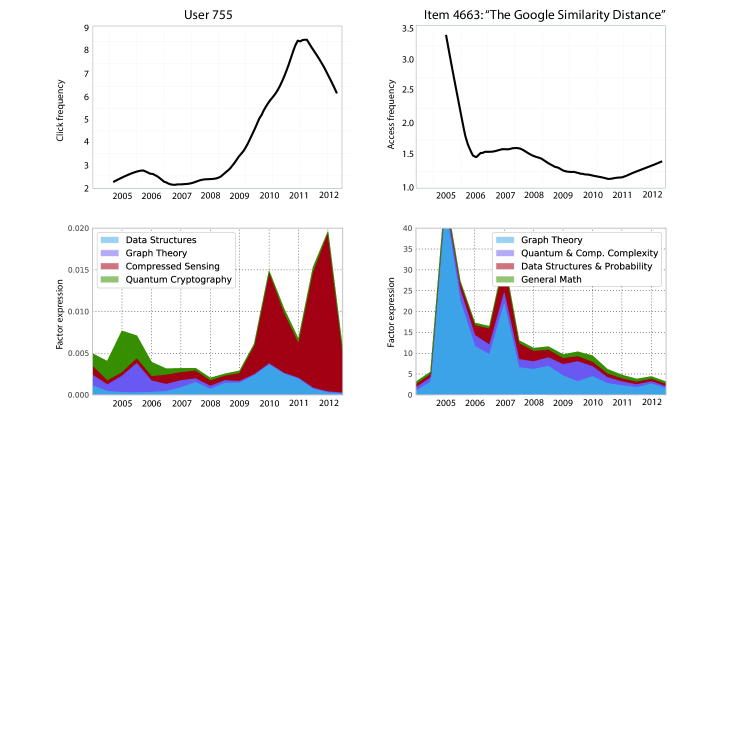
Figure 1: Our method, dPF, discovers evolving user interests and item audiences over time from raw click data. The top left plot shows the aggregate click frequencies for a user on arXiv.org for 8 years. dPF separates this aggregate data into a set of 20 interest groups with varying strengths over time (bottom left). This user was initially interested in quantum cryptography and graph theory; then, five years later, in compressed sensing and data structures. DPF decomposes raw access counts for items in a similar way. The top right plot shows the raw access frequencies for the paper “The Google Similarity Distance” (http://arxiv.org/pdf/cs/0412098.pdf). The bottom right plot indicates that the paper broadened its audience during its lifetime. It was initially popular only with graph theorists, then received attention from quantum physicists and computational complexity readers, perhaps explained by the fact that it was cited in “Google in a Quantum Network” (on arXiv and then in the Nature journal).

Related Work.   Several authors emphasize the importance of time modeling in collaborative filtering. These approaches differ in how they incorporate time information and their use of implicit data.

Koren [11] presents an approach based on matrix factorization that models the ratings as a product of user and item factors. This factorization is augmented with a user-item-time bias and user evolving factors. Our work is similar, but we allow for item-evolving factors to capture the possibility that item traits change over time (see Figure 1 for an example). Further, we provide a probabilistic framework for our model with approximate Bayesian inference to handle the considerable uncertainty that arises when modeling time evolving user behaviors. Similarly, Chatzis posits that only user membership to a discrete group (or class of users) evolves at each time-step, with new groups being created over time [4].

Some methods propose factorization of the user-item-time tensor [10, 19]. The intuition behind these methods is to project user and item factors into click space using a time-specific factor. These methods, rather than modeling the evolution of users and items over time, quantify the activity of each dimension of the factor model over time. Thus comparing the trajectories of specific users and items is impossible.

Gultekin and Paisley [7] propose modeling both user and item evolution with a Gaussian state-space model. For computational reasons, they perform a single forward (filtering) pass in time. In our work we show that we can perform both filtering and smoothing on large datasets. Similarly, Li et al. [14] use Dirichlet distributed latent factors, though they take a sampling-based inference approach that is not practical for real world datasets.

All the aforementioned methods are for explicit data. Two additional methods focus on implicit data, though with only user evolving preferences. Sahoo et al. [16] proposes an extension to the hidden Markov model where clicks are drawn from a negative binomial distribution. This discrete class-based approach requires many more classes to represent the same size of space that our additive factors achieve. Acharya et al. [1], constructed from gamma processes, has the advantage of inferring the dimensionality of the latent space, but takes an approach to inference that is not scalable and does not allow for item evolution. Our work is the first model that considers implicit data where both the users and items can evolve over time.

It is worth noting that recommendation frameworks to model general attributes, including context such as location and time, have also been proposed [15, 8]. In principle our work could be used to provide predictions within the framweork of Hidasi and Tikk [8].

2 Dynamic Poisson Factorization

In this section we review matrix factorization methods, Poisson matrix factorization, and introduce dynamic Poisson factorization.

Background: Matrix Factorization and Poisson Matrix Factorization.   The work of  Koren [11] is based on matrix factorization as are several of the other time-based methods highlighted at the start of this section. Matrix factorization aims at minimizing the distance between an approximation of the matrix, $U^{T}V$, and the original matrix $Y$ ($\text{dist}(Y,U^{T}V)$). This distance often has a probabilistic interpretation. Therefore, obtaining a good approximation (a small distance) can be cast as a maximum likelihood problem. For example, obtaining an approximation to the user-item matrix in terms of $l2$-loss is equivalent to assuming Gaussian noise on the observations. Similarly, $l2$ regularization of the optimization variables is equivalent to assuming Gaussian noise on the equivalent variables of a probabilistic model [2].

Expressing a model in probabilistic terms can reveal previously hidden perspectives. For example, a Gaussian distribution is not appropriate for modelling discrete observations (implicit clicks or explicit ratings) because its support is $\mathbb{R}$ and it places zero probability mass at any discrete point. Furthermore, probabilistic models come with powerful inference techniques rooted in Bayesian statistics. Machine learning using probabilistic models (graphical models) can be understood as a sequence of three steps: 1) posit a generative model of how the observations are generated; 2) condition on the observed data to infer posterior distributions of model’s unobserved (latent) variables; 3) use the posteriors according to the generative model to predict unobserved datum. In the context of matrix factorization, the Bayesian approach has been shown to produce superior predictions because it can average over many explanations of the data [17].

Poisson matrix factorization (PF) [6] addresses the mismatch between Gaussian models and the discrete observations. Poisson factorization assumes clicks are Poisson distributed and user/item factors are gamma distributed. This is another difference with respect to Gaussian factorization where factors are typically Gaussian distributed and can therefore be negative. Additively combining non-negative factors can lead to models that are easier to interpret [13]. Poisson factorization has been shown to outperform several types of matrix factorization models, including Gaussian matrix factorization, on recommendation tasks [6]. Furthermore, properties of the Poisson distribution allows the model to easily scale to massive real-life recommendation datasets.

Dynamic Poisson Factorization.   Poisson matrix factorization models users and items statically over time. This is unrealistic. For example, the preferences of the user in Figure 1 change from from “Graph Theory” and “Quantum Cryptography” to “Compressed Sensing”. Similarly, the readership of the item in Figure 1 evolves from “Graph Theory” to “Quantum & Computational Complexity” and “Data Structures & Probability”. To be able to capture both the changes of users and items over time, we introduce dynamic Poisson factorization (dPF).

DPF is a model of user-item clicks over time where time is assumed to be discrete (i.e., the modeler chooses a time window that aggregates clicks in chunks of 1 week, 1 month etc.). The aim is to capture the evolving preferences of users as well as the evolution of item popularity over time. Specifically, dPF models a set of users clicking, or rating, a set of items over time.

We first give a high-level overview of dPF. The strengths of user preferences and item popularities are assumed to be a combination of static and dynamic processes. The static portion assigns each user and item a time-independent representation, while the dynamic portion gives each user and item a time evolving model. The static representation is the same as in traditional matrix factorization approaches and captures the baseline interest of users and the baseline popularity of items, which is then modified by dynamic variables. In this respect, dPF is a generalization of PF [6].

We now give the mathematical details for how to capture this intuition in a model. To model time probabilistically, statisticians typically use Gaussian time series models called state space models [2]. In the simplest case, state space models draw the state at the next time step from a Gaussian with mean equal to the previous time step and fixed variance $\sigma^{2}$:

$$x_{t}|x_{t-1}\sim\mathcal{N}(x_{t-1},\sigma^{2}).$$

We use state space models as the dynamic portion of dPF, where both the users and items evolve. Formally, $u_{nk,t}$, the $k$th component of the $n$th user at time $t$ is constructed as

$$u_{nk,t}|u_{nk,t-1}\sim\mathcal{N}(u_{nk,t-1},\sigma_{u}^{2}).$$

The state space process for items is symmetric. The static components associated with each user $u_{nk}$ and item $v_{mk}$ are also drawn from a normal distribution. They form the intercepts for a time evolving factorization with Poisson observations. That is, a user’s expression of factor $k$ at time $t$ is the sum $\bar{u}_{nk}+u_{nk,t}$. In this sense, the state space model can be viewed as governing correction factors and thus capture the evolution of users’ preferences through time, while static global factors capture the interest of users that are not influenced by time.

One issue in using Gaussian state space models is that Poisson observations have non-negative parameters (rates). Thus, we exponentiate the state-space models intercept sums for each user and item before combining them to form the mean of the observed rating. Concretely, the rating for user $n$, item $m$ at time $t$, $y_{nm,t}$ has the following distribution

$$y_{nm,t}\sim\text{Poisson}(\sum_{k=1}^{K}e^{(u_{nk,t}+\bar{u}_{nk})}e^{(v_{mk,t}+\bar{v}_{mk})}).$$

Putting this all together, the observations are drawn as follows:

1. Draw user global factors: $\bar{u}_{nk}\sim\mathcal{N}(\mu_{\bar{u}},\sigma_{\bar{u}}^{2})$

2. Draw item global factors: $\bar{v}_{mk}\sim\mathcal{N}(\mu_{\bar{v}},\sigma_{\bar{v}}^{2})$

3. For each time step: $t=1\ldots T$

   • Draw user and item correction factors:

   • if $t=1$

   • $u_{nk,1}\sim\mathcal{N}(\mu_{u},\sigma_{u}^{2})$

   • $v_{mk,1}\sim\mathcal{N}(\mu_{v},\sigma_{v}^{2})$

   • else

   • $u_{nk,t}|u_{nk,t-1}\sim\mathcal{N}(u_{nk,t-1},\sigma_{u}^{2})$

   • $v_{mk,t}|v_{mk,t-1}\sim\mathcal{N}(v_{mk,t-1},\sigma_{v}^{2})$

   • Draw a click:

   • $y_{nm,t}\sim\text{Poisson}(\sum_{k=1}^{K}e^{(u_{nk,t}+\bar{u}_{nk})}e^{(v_{mk,t}+\bar{v}_{mk})})$

Unlike Poisson matrix factorization [6] our model uses Gaussian-distributed (global) user and item factors. We could have also used Gamma-distributed factors [1] although the parametrization of Gaussians allows us to independantly control the mean and variance of each Gaussian in the chain. Further, even with this change, dPF can still model the long-tail of users and items, an important advantage of Poisson factorization over Gaussian matrix factorization [6].

Analysis and Predictions.   We analyze data through the posterior, $p(u,\bar{u},v,\bar{v}|Y)$. We use $u$ to represent the set of all user factors and $Y$ the observations. The posterior distribution places probability mass on the latent variables in proportion to how well they explain the observations. The posterior of standard Poisson factorization finds a single set of preferences and attributes, while the dPF posterior places high probability on the sequences of preferences and attributes that best describe the observed data. Figure 1 plots the expected value under the posterior distribution of the expression of factor $k$ by user $n$, $u_{nk,t}+\bar{u}_{nk}$, and the similar posterior expectation for the items.

In recommendation applications, one wants to use the model to predict the value of unobserved clicks. We obtain predictions by taking the inner product of the expected value of the user factors and item factors under the posterior distribution:

$$\text{E}[y_{nmt}|Y]\approx\sum_{k}\text{E}_{\textrm{posterior}}[e^{(u_{nk,t}+\bar{u}_{n,k})}e^{(v_{mk,t}+\bar{v}_{m,k})}].$$ (1)

In practice, recommender systems require rankings (e.g., to show users their top 10 most recommended items when they log on to a website, or to auto-play the most recommended video when the current video has finished). To calculate rankings we use the predictive distribution in Equation 1 as a score for each unobserved rating triplet (i.e., higher predictive probability results in a higher score) and sort the triplets by these scores.

Computation.   We approximate the posterior distribution with variational inference, which transforms the posterior estimation problem into an optimization problem. In Appendix A we provide the variational inference algorithm for dPF. The per iteration complexity of performing posterior inference for dPF is $O(T(R+NK+MK))$ where $R$ is the number of non-zero observations of the most populous time step ($R=\max_{t}R_{t}$), $T$ the number of time steps, $N$ and $M$ the number of users and items, and K the number of latent components respectively.

The updates of each factor depend only on the other factors in its Markov blanket (a factor’s parents, its children, and its children’s parents). As a consequence, the updates to the variational parameters of each user are independent of all other users (and similarly for items). Hence we can easily parallelize the posterior inference computations. We implement dPF in C++ and use openMP for parallelization. Empirically, we obtain a near linear speedup in the number of threads.

Implementation Details.   We initialize hyperparameters ($\mu_{u},\mu_{v},$ $\bar{\mu}_{u},\bar{\mu}_{v}$) controlling the means to the priors to small random numbers close to 0 and variance hyperparameters ($\sigma_{u},\sigma_{v},\sigma_{\bar{u}},\sigma_{\bar{v}}$) to 10. We found that these values work well across different datasets. We provide indications that the model is well-behaved under a wide range of hyperparameter settings (Section 3). We have found that for interpretability, it is important to use the same initialization for factors across time. We experimented with initializing the global factors with PF but that did not provide an advantage. We ran the the numerical optimization routines for up to 500 iterations or until convergence.

3 Experiments

We now fit our model using datasets consisting of users consuming movies and scientists clicking on papers. As we describe in Section 2 we can use the expectation of the posterior distributions over user and item latent factors to provide item recommendations to users through time. In addition to measuring the performance of dPF against baselines we gain insights into the datasets and the model by exploring its posteriors. We highlight the following results:

1. dPF provides better recommendations across multiple datasets compared to several static and dynamic baselines.

2. dPF scales to large datasets.

3. dPF allows us to explore and gain interesting insights into the arXiv dataset.

In Section 3.1, we describe the two datasets used in our experiments. We then formalize the experimental methodology and the comparative metrics in Section 3.2. Finally, we provide comparative and explorative results in Sections 3.3, 3.4, and 3.5.

3.1 Datasets

We study two different datasets.

Netflix-time: First, we consider a movie dataset derived from the Netflix challenge. We follow a similar procedure as described in Li et al. [14] to obtain a subset of the original Netflix dataset focusing on users and movies that have been active over several years. The resulting dataset contains 7.5K users, 3.6K items, and 2 million non-zero observations over 14 time steps (with a granularity of 3 months). The validation and test sets are composed of all the clicks occurring in the final 9 months of the dataset (90K clicks). Since our focus is on the implicit data case, we binarize the data such that every observed rating is a “1” rating and all unobserved ratings are zeros.

Netflix-full: In addition to the Netflix-time dataset, we fit dPF on the whole Netflix dataset (with a granularity of 6 months) where we kept the last 1.5 years of click for validation and test. The resulting dataset contains over 225K users and 14K items and 6.9M observations. This dataset is more challenging for inference because it includes items in the long tail (i.e., a large number of items used by very few users) and very inactive users.

arXiv: DPF is also fit on a click data from the arXiv.org site. arXiv.org is a pre-print server for scientific papers. We have access to ten years of clicks from registered users of arXiv. We keep 75K papers with at least 20 clicks over the ten years and 5K users with clicks spanning at least five years (1.3M observations). We set the time granularity to be six months which seems reasonable to capture scientists’ changing preferences. We verified that the results are similar with other time periods. The resulting dataset contains 19 time periods. We keep all observations of the last time step (the last six months) for validation and testing.

arXiv-cs-stats: Physicists were early adopters of the arXiv. As such, fits to the above dataset are dominated by that field. To gain insights into our model’s discoveries we have found it useful to restrict our attention to subject areas that were closer to our computer science expertise. This dataset is a cut of the data with papers that are in either computer science (CS) or statistics (Stats) fields. The field(s) of each paper is selected by its authors when submitting. The resulting data has just under 1K users, 5K items and spans 7 years worth of clicks (58K observations). We use this data for explorative purposes (Section 3.5).

3.2 Baselines

We are able to compare to BPTF, a recently-proposed dynamic model based on tensor factorization approach. Xiong et al. [19] model the changing strengths of factors over time with a probabilistic tensor approach. In more detail, the observation matrix is assumed to decompose into a tensor product between user preferences, item popularities, and temporal trends. Their approach captures aggregate changes in behavior but is not specific enough to model the time-dependent shifts of individual users or items. They use Gibbs sampling to infer the latent factors given explicit data only, an approach that does not scale when considering implicit data on larger datasets. To adapt this method to the implicit data case we sampled a random subset of unobserved items such as to observe an equal number of zeros and ones.

Another natural benchmark to demonstrate the benefits of time modelling is Poisson matrix factorization, since our model builds on that approach.

An effective time model should be able to learn how to weight the different clicks based on recency and retain the information from older clicks only to the extent that it is useful to predict new ones. For example, in a system where user preferences quickly evolve, the system may rapidly forget about older preferences. To clearly demonstrate the benefits of time modelling we compare to two different PF models. The first is trained using all past ratings (PF-all) while the second is trained using only observations at the last (train) time period (PF-last).

We note that the implicit data case is significantly more challenging than the usual explicit data case. First, the observations are extremely imbalanced. For example in the datasets used in the experiments “0” observations outnumber “1” observations by a ratio of over 250 to 1 (arXiv). Second, implicit data methods train on exactly $NM$ observations. Finding baselines that will scale to these data sizes is challenging. Furthermore, our focus on implicit data means that we cannot readily compare to previously published results.

We also fit the popular TimeSVD++ model [11]. It is not designed for the implicit data case and preliminary experiments (where we studied different methods of incorporating zero observations) on our Netflix-time dataset showed that it performed significantly worse than all baselines (including both static PF models).

For all experiments we set the number of components to $K=20$. Our results generalize beyond this value.

3.3 Click prediction & Metrics

We simulate a realistic scenario where each method is given access to past user clicks and the models must predict items of future interest to the users. Further for each dataset we repeat this process for each time step. That is for each time step $t$ we train with all observations before $t$ (i.e., $1\ldots t-1$) and evaluate predictions on the observations at $t$. When reporting results we average over all time steps.

Evaluating the accuracy of a collaborative filtering model for implicit data is usually done using ranking-related error metrics. We consider user recall given K top-items to recommend (“recall@K” see below for details). However, we notice that on datasets containing many items, models often fail to place any of the user’s consumed items in the top K. These metrics limit our ability to understand the merits of different models. As a remedy we turn to metrics which take into account all test items while discounting the contribution of an item as a function of its predicted rank. The popular NDCG, and mean reciprocal rank (MRR) both have this property. MRR linearly decays the relevance of an item as a function of its rank while NDCG logarithmically decays them. We also report the mean average rank (MAR) metric.

Formally, for binary data the four chosen metrics are:

• - Recall@T: $\frac{1}{N}\sum_{i=1}^{N}\sum_{j\in\in\mathbf{y}_{i}^{U}}\frac{\mathbf{I}(\text{rank}(i,j)\leqslant T)}{\text{min}(T,|\mathbf{y}_{i}^{U}|)}$
  where $\mathbf{I}$ is the indicator function. In our experiments we set T to 50 for all datasets which is a reasonable number of items to present to a user. Results are consistent across other values of T that we have studied.

• - Normalized discounted cumulative gain (NDCG):
  $\frac{1}{N}\sum_{i=1}^{N}\sum_{j\in\mathbf{y}_{i}^{U}}\frac{1}{\log(\text{rank}(i,j)+1)}$.

• - Mean reciprocal rank (MRR): $\frac{1}{N}\sum_{i=1}^{N}\sum_{j\in\mathbf{y}_{i}^{U}}\frac{1}{\text{rank}(i,j)}$.

• - Mean average rank (MAR): $\frac{1}{N}\sum_{i=1}^{N}\sum_{j\in\mathbf{y}_{i}^{U}}\text{rank}(i,j)$.

$\mathbf{y}_{i}^{U}$ is the set containing user $i$’s test observations and $N$ the number of users. $\text{rank}(i,j)$ is the predicted rank of item $j$ for user $i$.

3.4 Results

The results across all datasets consistently show the superior performance of dPF according to all baselines. Below we examine these results in more detail.

We first turn our attention to the Netflix data. On the Netflix-time dataset dPF outperforms all baselines according to all metrics (Table 1). We note that the BPTF baseline mostly outperforms PF-all and PF-last. This indicates that while BPTF’s time model is useful, modeling users’ and items’ individual evolutions is preferable.

The performance on Netflix-full is similar where dPF also outperforms all baselines. Other authors have shown that outperforming static models on Netflix is challenging [19]. As outlined in Koren [11], Netflix users who change at a very fine level of granularity (daily) may be hard to capture with a coarser granularity. Furthermore, we note that users who rarely use the service do not provide enough data to disambiguate between a small number of changing user interests and a wider number of static user interests that happen to be exhibited over many time steps (a similar argument applies to movies in the long tail). Nonetheless dPF is able to slightly outperform static methods by capturing evolving preferences and viewer ship where available.

Fitting BPTF to this larger dataset is prohibitively expensive even with our proposed subsampling approach. As such we could not report results on the larger Netflix dataset nor on the arXiv dataset.

The arXiv is a good testbed for our model since scientists and science evolve and we believe that it may be possible to capture such evolutions using arXiv’s click data. We note that dPF outperforms all other methods on arXiv (Table 3). This further validates that dPF provides better recommendations by modelling the evolution of users and items.

From a methodological point of view it is also interesting to note that there is not always perfect correlation between all the metrics (that is the rank of the baselines change under different metrics). Amongst them MAR seems to be noisiest metric. It can probably be explained by the fact that it is less robust to outliers because it weights every test observation evenly.

	Recall@50	MAR	MRR	NDCG
dPF	0.170	640	0.027	0.294
BPTF [19]	0.148	668	0.020	0.277
PF-all [6]	0.145	691	0.021	0.280
PF-last [6]	0.065	807	0.019	0.268

Table 1: Performance of dPF versus baselines on Netflix-time. Bold numbers indicate the top performance for each metric. We were unable to obtain competitive performance from TimeSVD++[11].

	Recall@50	MAR	MRR	NDCG
dPF	0.156	1605	0.021	0.358
PF-all [6]	0.120	1807	0.015	0.338
PF-last [6]	0.138	1635	0.018	0.351

Table 2: Performance of dPF versus PF on the Netflix-full dataset. Bold numbers indicate the top performance for each metric. While dPF does best according to all metrics, PF-last slightly outperforms PF-all. The performance of PF-last seems to indicate that user preferences and movie popularities vary rapidly.

	Recall@50	MAR	MRR	NDCG
dPF	0.035	21822	0.0062	0.186
PF-all [6]	0.032	22402	0.0056	0.182
PF-last [6]	0.023	25616	0.0040	0.168

Table 3: Performance of dPF versus baselines on arXiv. Bold numbers indicate the top performance for each metric.

Effect of hyperparameter values.  

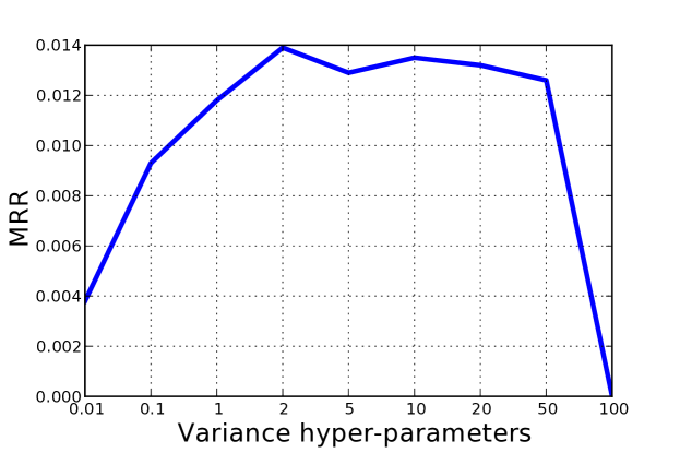
Figure 2: dPF performs well across a large range of variances (2–50) by MRR in a pilot study of a single timestep of the arXiv data.

We have found that dPF is fairly robust to the values of its hyperparameters. We demonstrate it more formally for the variance hyperparameters (Figure 2). We note that except at the extremes the performance of dPF is good for a wide-range of variances. In our experimental setup the last time step is used for predictions. This can may explain the model’s robustness.

Figure 3: Evolution of latent factors, corresponding to research areas, as discovered by dPF from the raw click data. We see that network analysis has been a growing area of research in computer science over the past decade.

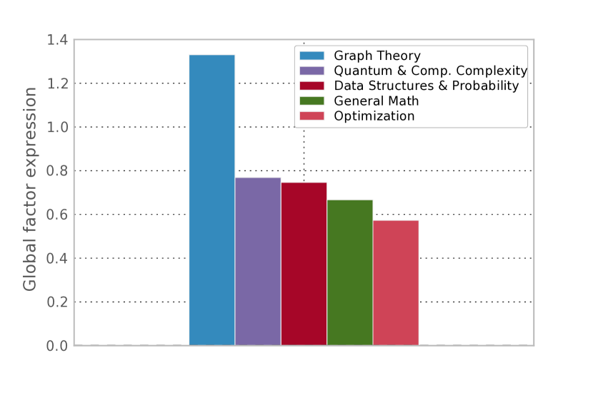
Figure 4: The expression level of five static factors of “The Google Similarity Distance” paper. When compared to the dynamic trend in Figure 1, we see that the static factors identify the paper’s main field, graph theory. Moreover, dPF can use the local factors to express excursions to other fields.

3.5 Exploration

There are various ways of evaluating a probabilistic model. While we have provided conclusive empirical results above we now turn to exploration of the model’s posteriors. Exploring the posterior can be a useful diagnosis tool [3]. Here our aim is to further validate our modelling choices. We also want to better understand the arXiv-cs-stats dataset.

In Figure 1 we showed, using the local expected value of its factors under their posterior distribution, an item that garnered interest from different communities over time. We can also examine the model’s global expected value under the posterior distribution (Figure 4). In addition to the four factors in Figure 1 we added an extra factor (labeled “Optimization”) which is unused by this paper. The “Graph Theory” factor is the highest global factor, which is sensible since it expresses the paper’s main field. The other three factors are expressed at levels which are in between “Graph Theory” and “Optimization”. The global popularity of this paper in these four fields is the same. In particular, dPF can simply use local factors to explain ephemeral popularity in other fields.

In addition to looking at single users and items we can explore the model at the aggregate level to discover global patterns. For example, we can look at the evolution of different scientific fields over time. We plot the expected value of all 20 factors inferred using the arXiv-cs-stats dataset (Figure 3). We corrected for arXiv’s growing popularity over time. Scientific fields on arXiv are all well established, and as such, their popularities are stable over time. Note that this does not mean that fields do not evolve. We also notice that according to dPF, some fields have gained in popularity (in particular “Machine Learning & Information Theory” as well as “Networks & Society”).

4 Conclusions & Future Work

We examined the problem of modelling user-item clicks through time. Our main contribution is the dynamic Poisson factorization model (dPF). In addition to modeling both users and items changing through time and being able to scale to large datasets using implicit information, we showed the empirical advantages of modelling the evolution of users and items. Importantly we used this model to explore and better understand the arXiv, an indispensable tool to many scientific fields.

There are several opportunities to extend this work. It would be interesting to model aggregate user trajectories to better understand how (scientific) communities evolve. It would also be worthwhile to allow users and items to be modelled at multiple different granularities. This would allow a model to understand both short and long-term evolutions. Although we can set the granularity in our current computation (and memory consumption) may become an issue as the granularity gets small. Continuous time models may offer interesting avenues to avoid specifying granularities.

Acknowledgements.   We thank the reviewers for their helpful comments. RR is supported by an NDSEG fellowship. DMB is supported by NSF IIS-0745520, NSF IIS-1247664, ONR N00014-11-1-0651, and DARPA FA8750-14-2-0009.

Appendix A Inference

Performing Bayesian inference on the random variables of dPF requires calculating the posterior distribution. This is difficult due to the non-conjugacy (lack of analytic integrals) between the log-normal distribution of the factors and the Poisson-distributed observations. We therefore resort to approximate inference techniques (e.g., Markov chain Monte Carlo or variational methods).

Variational inference frames the posterior inference task as the problem of minimizing the KL-divergence between an approximate distribution and the true posterior. This optimization approach is orders of magnitudes faster than sampling-based approaches, at the cost of not being able to capture the full Bayesian posterior. We assume that our approximating family (in variational inference) fully factorizes. The variational distribution of individual factors is normally-distributed:

$$q(\mathbf{u}_{nt}) = \prod_{k}q(u_{nt,k}|\hat{\mu}_{unt,k},\hat{\sigma}_{unt,k}^{2})$$

$$= \prod_{k}\mathcal{N}(u_{nt,k}|\hat{\mu}_{unt,k},\hat{\sigma}_{unt,k}^{2})$$

We treat the other time-independent ($v$) and time-dependent ($\bar{u}$ and $\bar{v}$) latent variables in a similar way. To differentiate the variables of the generative model from their variational counterparts we denote the latter with a circumflex (a “hat”).

It is straightforward to show that minimizing the KL-divergence between the q distribution and the true posterior is equivalent to maximizing a lower bound on the model’s log evidence [9]. We use the bold symbols to denote sets of factors, for example the set of all user factors: $\mathbf{u}\equiv\{u_{nt,k}\}_{n=0:N,t=1:T}$. $\zeta$ stands for the set of all hyperparameters: $\{\mu_{u},\sigma_{u},\mu_{v},\sigma_{v},\mu_{\bar{u}},\sigma_{\bar{u}},\mu_{\bar{v}},\sigma_{\bar{v}}\}$. $\lambda$ denotes all of the parameters to the variational distribution such as $\hat{\mu}_{unk,t}$ and $\hat{\sigma}_{unk,t}^{2}$. For our model, this evidence lower bound (ELBO) is

$$p(\mathbf{y}|\zeta) \geqslant{\cal L}(\lambda)$$ (2)

$$:=\text{E}_{q}[\log p(\mathbf{y},\mathbf{u},\mathbf{v},\mathbf{\bar{u}},\mathbf{\bar{v}}|\zeta)]-\text{E}_{q}[\log q(\mathbf{u},\mathbf{v},\mathbf{\bar{u}},\mathbf{\bar{v}})].$$

The fully-factorized approximation allows us to expand the ELBO as follows:

$$\sum_{n}^{N}\text{E}_{q}[\log p(\mathbf{\bar{u}}_{n}|\bm{\mu}_{\bar{u}},\sigma^{2}_{\bar{u}}\mathbf{I})]+\sum_{m}^{M}\text{E}_{q}[\log p(\mathbf{\bar{v}}_{m}|\bm{\mu}_{\bar{v}},\sigma^{2}_{\bar{v}}\mathbf{I})]$$

$$+\sum_{t=2,n}^{T,N}{\text{E}_{q}[\log p(\mathbf{u}_{n,t}|\mathbf{u}_{n,t-1},\sigma_{u}^{2}\mathbf{I})]}+\sum_{n}^{N}{\text{E}_{q}[\log p(\mathbf{u}_{n,1}|\bm{\mu}_{u},\sigma_{u}^{2}\mathbf{I})]}$$

$$+\sum_{t=2,m}^{T,M}{\text{E}_{q}[\log p(\mathbf{v}_{m,t}|\mathbf{v}_{m,t-1},\sigma_{v}^{2}\mathbf{I})]}+\sum_{m}^{M}{\text{E}_{q}[\log p(\mathbf{v}_{v,1}|\bm{\mu}_{v},\sigma_{v}^{2}\mathbf{I})]}$$

$$+\sum_{n,m,t}^{N,M,T}{\text{E}_{q}[\log p(y_{nm,t}|\sum_{k}exp(u_{nk,t}+\bar{u}_{nk})^{T}exp(v_{mk,t}+\bar{v}_{mk}))]}$$

$$+{H(q)}$$

where $H(q)$ is the entropy of the variational distribution.

To optimize the ELBO one typically expands the expectations in Equation A. The variational parameters can then be optimized using coordinate or gradient ascent. The non-conjugacy in our model implies that further manipulations are required to express the expectations from Equation A in closed form. In particular the term requiring an additional approximation comes from the Poisson distribution. The Poisson pdf, with rate $\lambda$ is $\frac{\lambda^{k}}{k!}e^{-\lambda}$. The first term in the ELBO as expressed in Equation A (the joint distribution over latent and observed variables) can be re-written using the product rule of probability as:

$$\text{E}_{q}[\log p(\mathbf{y}|\mathbf{u},\mathbf{v},\mathbf{\bar{u}},\mathbf{\bar{v}})+\log p(\mathbf{u},\mathbf{v},\mathbf{\bar{u}},\mathbf{\bar{v}}|\zeta)].$$

The first term corresponds to the Poisson distribution. It can be expanded into:

$$\text{E}_{q}[\log\frac{\lambda^{k}}{k!}\exp^{-\lambda}] =\text{E}_{q}[k\log\lambda-k!-\lambda]$$

$$=\text{E}_{q}[k\log\lambda]-\text{E}_{q}[\lambda]-k!$$

where $\lambda=\sum_{k}\exp(u_{nk,t}+\bar{u}_{nk})\exp(v_{mk,t}+\bar{v}_{mk})$. We do not know of a closed-form exact solution to the first expectation when $k$ is non-zero. Fortunately several known techniques can be used to approximate this integral [18]. We re-use an idea from the recent Poisson factorization which consists of adding a set of auxiliary random variables. For dPF, this means adding auxilliary variables $\phi_{mnt,k}$ one for each user-item-timestep component for all of the non-zero ratings. Formally, this allows for the following manipulation:

$$\log\sum_{k}\exp(u_{nk,t}+\bar{u}_{nk})\exp(v_{mk,t}+\bar{v}_{mk})$$ (3)

$$=\log\sum_{k}\frac{\phi_{nmk,t}}{\phi_{nmk,t}}\exp(u_{nk,t}+\bar{u}_{nk})\exp(v_{mk,t}+\bar{v}_{mk})$$ (4)

$$=\log\text{E}_{\mathbf{\phi}}[\frac{\exp(u_{nk,t}+\bar{u}_{nk})\exp(v_{mk,t}+\bar{v}_{mk})}{\phi_{nmk,t}}]$$ (5)

$$\geqslant\text{E}_{\mathbf{\phi}}[u_{nk,t}+\bar{u}_{nk}+v_{mk,t}+\bar{v}_{mk}-\log\phi_{nmk,t}]$$ (6)

We obtain the last inequality by applying Jensen’s inequality. We note that, unlike in Poisson factorization, the resulting model is not conditionally conjugate, which intuitively means the distribution of a variable given everything else has known form. As a result, the equations do not yield closed-form updates. We use numerical optimization and perform coordinate ascent on the ELBO using a quasi-Newton optimizer (L-BFGS). The update for $\phi_{nmt,k}$ can be solved for in expected value with respect to $q$ of Eq. LABEL:eq:double-jensen as

$$\phi_{nmk,t}\propto\exp(\hat{u}_{nk,t}+\hat{\bar{u}}_{nk}+\hat{v}_{mk,t}+\hat{\bar{v}}_{mk})$$ (8)

The algorithm used to infer the variational posteriors (i.e., train the model) is shown in Figure 5.

• For $t=1\ldots T:$

  • Update $\hat{\mu}_{unk,t}\text{ and }\hat{\sigma}_{unk,t}\text{with L-BFGS using}\nabla_{\hat{\mu}_{unk,t},\hat{\sigma}_{unk,t}}{\cal L}\;\;\forall n,k$

  • Update $\hat{\mu}_{vmk,t}\text{ and }\hat{\sigma}_{vmk,t}\text{with L-BFGS using}\nabla_{\hat{\mu}_{vmk,t},\hat{\sigma}_{vmk,t}}{\cal L}\;\;\forall m,k$

  • Update $\hat{\phi}_{nmk,t}\;\;\forall n,m,k,t\mid y_{n,mt}>0$ using Eq. 8

• Update $\hat{\mu}_{\bar{u}n,k}\text{ and }\hat{\sigma}_{\bar{u}n,k}\text{with L-BFGS using}\nabla_{\hat{\mu}_{\bar{u}n,k},\hat{\sigma}_{\bar{u}n,k}}\;\;\forall n,k$

• Update $\hat{\mu}_{\bar{v}m,k}\text{ and }\hat{\sigma}_{\bar{v}m,k}\text{with L-BFGS using}\nabla_{\hat{\mu}_{\bar{v}m,k},\hat{\sigma}_{\bar{v}m,k}}{\cal L}\;\;\forall m,k$

• Repeat until convergence

Figure 5: Coordinate ascent algorithm for dPF. We first update the (variational) correction factors and subsequently we update the (variational) global factors. Prior to each update the corresponding vector $\bm{\phi}_{nmt}$ must be evaluated.

References

- Acharya et al. [2015] A. Acharya, J. Ghosh, and M. Zhou. Nonparametric bayesian factor analysis for dynamic count matrices. In Proceedings of the 18th Conference on Artificial Intelligence and Statistics, 2015.
- Bishop [2006] C. M. Bishop. Pattern Recognition and Machine Learning. Springer, 2006.
- Blei [2014] D. M. Blei. Build, compute, critique, repeat: Data analysis with latent variable models. Annual Review of Statistics and Its Application, 1(1):203–232, 2014. 10.1146/annurev-statistics-022513-115657.
- Chatzis [2014] S. Chatzis. Dynamic bayesian probabilistic matrix factorization. In Proceedings of the Twenty-Eighth AAAI Conference on Artificial Intelligence, 2014., pages 1731–1737, 2014.
- Ekstrand et al. [2011] M. D. Ekstrand, J. T. Riedl, and J. A. Konstan. Collaborative filtering recommender systems. Foundations and Trends in Human-Computer Interaction, 4(2):81–173, 2011.
- Gopalan et al. [2015] P. Gopalan, J. Hofman, and D. Blei. Scalable recommendation with hierarchical poisson factorization. In Proceedings of the Thirti-first Conference Annual Conference on Uncertainty in Artificial Intelligence (UAI-15). AUAI Press, 2015.
- Gultekin and Paisley [2014] S. Gultekin and J. Paisley. A collaborative kalman filter for time-evolving dyadic processes. In 2014 IEEE International Conference on Data Mining, ICDM, 2014, pages 140–149, 2014.
- Hidasi and Tikk [2015] B. Hidasi and D. Tikk. General factorization framework for context-aware recommendations. Data Mining and Knowledge Discovery, pages 1–30, 2015. ISSN 1384-5810.
- Jordan [1999] M. I. Jordan, editor. Learning in Graphical Models. MIT Press, Cambridge, MA, USA, 1999. ISBN 0-262-60032-3.
- Karatzoglou et al. [2010] A. Karatzoglou, X. Amatriain, L. Baltrunas, and N. Oliver. Multiverse recommendation: n-dimensional tensor factorization for context-aware collaborative filtering. In Proceedings of the fourth ACM conference on Recommender systems, pages 79–86. ACM, 2010.
- Koren [2010] Y. Koren. Collaborative filtering with temporal dynamics. Commun. ACM, 53(4):89–97, 2010.
- Koren and Sill [2011] Y. Koren and J. Sill. Ordrec: an ordinal model for predicting personalized item rating distributions. In Proceedings of the fifth ACM conference on Recommender systems, pages 117–124, 2011.
- Lee and Seung [1999] D. D. Lee and H. S. Seung. Learning the parts of objects by non-negative matrix factorization. Nature, 401(6755):788–791, 10 1999.
- Li et al. [2011] B. Li, X. Zhu, R. Li, C. Zhang, X. Xue, and X. Wu. Cross-domain collaborative filtering over time. In Proceedings of the Twenty-Second International Joint Conference on Artificial Intelligence - Volume Volume Three, IJCAI’11, pages 2293–2298. AAAI Press, 2011.
- Rendle [2010] S. Rendle. Factorization machines. In Proceedings of the 10th IEEE International Conference on Data Mining. IEEE Computer Society, 2010.
- Sahoo et al. [2012] N. Sahoo, P. V. Singh, and T. Mukhopadhyay. A hidden markov model for collaborative filtering. MIS Q., 36(4):1329–1356, Dec. 2012.
- Salakhutdinov and Mnih [2008] R. Salakhutdinov and A. Mnih. Bayesian probabilistic matrix factorization using Markov chain Monte Carlo. In Proceedings of the International Conference on Machine Learning, volume 25, 2008.
- Wang and Blei [2013] C. Wang and D. Blei. Variational inference in nonconjugate models. Journal of Machine Learning Research, 14:1005–1031, 2013.
- Xiong et al. [2010] L. Xiong, X. Chen, T.-K. Huang, J. Schneider, and J. G. Carbonell. Temporal collaborative filtering with bayesian probabilistic tensor factorization. In Proceedings of SIAM Data Mining, 2010.
- Yi et al. [2014] X. Yi, L. Hong, E. Zhong, N. N. Liu, and S. Rajan. Beyond clicks: dwell time for personalization. In Proceedings of the 8th ACM Conference on Recommender systems, pages 113–120, 2014.