The Shape of Data and Probability Measures

Abstract

We introduce the notion of multiscale covariance tensor fields (CTF) associated with Euclidean random variables as a gateway to the shape of their distributions. Multiscale CTFs quantify variation of the data about every point in the data landscape at all spatial scales, unlike the usual covariance tensor that only quantifies global variation about the mean. Empirical forms of localized covariance previously have been used in data analysis and visualization, for example, in local principal component analysis, but we develop a framework for the systematic treatment of theoretical questions and mathematical analysis of computational models. We prove strong stability theorems with respect to the Wasserstein distance between probability measures, obtain consistency results for estimators, as well as bounds on the rate of convergence of empirical CTFs. These results show that CTFs are robust to sampling, noise and outliers. We provide numerous illustrations of how CTFs let us extract shape from data and also apply CTFs to manifold clustering, the problem of categorizing data points according to their noisy membership in a collection of possibly intersecting smooth submanifolds of Euclidean space. We prove that the proposed manifold clustering method is stable and carry out several experiments to illustrate the method.

1 Introduction

Probing, analyzing and visualizing the shape of complex data are challenges that are magnified by the intricate dependence of their structural properties, as basic as dimensionality, on location and scale (cf. [1]). As such, resolving and integrating the geometry and topology of data across scales are problems of foremost importance. In this paper, we develop the notion of multiscale covariance tensor fields (CTF) associated with Euclidean random variables and show that many properties of the shape of their distributions become accessible through CTFs, which provide stable representations that can be estimated reliably from data.

For a random vector $y\in\mathbb{R}^{d}$, scale dependence is controlled by a kernel function $K(x,y,\sigma)\geqslant 0$, where $x,y\in\mathbb{R}^{d}$ and $\sigma>0$ is the scale parameter. The idea is that from the standpoint of $x$, at scale $\sigma>0$, the kernel masks the distribution by attributing weight $K(x,y,\sigma)$ to data located at $y$, creating a windowing effect. More simply put, $K(x,y,\sigma)$ quantifies how well an observer at $x$ sees data at $y$ at scale $\sigma$. Covariation of the weighted data is measured relative to every point $x\in\mathbb{R}^{d}$, not just about the mean as is common practice, thus giving rise to a multiscale covariance field. Special cases of these covariance fields were introduced in [2], targeting applications to such problems as detection of local scales and feature rich points in shapes. Here we present a more systematic treatment that includes a broader formulation of multiscale CTFs, stability theorems that ensure that properties of probability measures derived from multiscale CTFs are robust, as well as consistency results and convergence rates for empirical CTFs. We prove stability of CTFs with respect to the Wasserstein distance between probability measures, a metric that is finding uses in an ever expanding landscape of problems and whose origins are in optimal transport theory [3, 4]. Since Wasserstein distance metrizes weak convergence of probability measures, we obtain a strong stability result that ensures that if two probability distributions are similar in a weak sense, then their multiscale CTFs are uniformly close over the entire domain. Convergence rates are derived from the stability theorems and results by Fournier and Guillin [5] and García-Trillos and Slepčev [6] on convergence of empirical measures. The standard covariance tensor of a random vector $y\in\mathbb{R}^{d}$ quantifies covariation of $y$ about the mean, but may be extended to a full covariance field by considering covariation about arbitrary points. Nonetheless, this field provides no information about the organization of the data other than that already contained in the covariance about the mean. Thus, a localized formulation is essential for gaining additional insight into the shape of data.

The trace of a multiscale CTF is a scalar field that gives a multiscale analogue of the classical Fréchet function $V(x)=\mathbb{E}\left[\|y-x\|^{2}\right]$ of a random variable $y$ with finite second moment. The Fréchet function provides a more geometric interpretation of the mean as the unique minimizer of $V$; that is, the point $\mu\in\mathbb{R}^{d}$ with respect to which the spread of $y$ is minimal. Similarly, the local extrema and other properties of the multiscale Fréchet function provide a wealth of information about the distribution of $y$. In fact, we show that the distribution of any random vector may be fully recovered from the multiscale Fréchet function associated with the Gaussian kernel.

Several variants of empirical localized or weighted covariance previously have been used in data analysis, but we develop a framework for the formulation and systematic treatment of such problems. Allard et al. have developed a computational model termed geometric multi-resolution analysis for multiscale data analysis based on covariance localized to hierarchies of dyadic cubes [7]. In computer graphics, local principal component analysis (PCA) is commonly used in the estimation of normals to surfaces from point-cloud data [8] for surface reconstruction; see also [9] and references therein. In computer vision, tensor voting by Medioni et al. [10] has been applied to multiple image analysis and processing tasks. Brox et al. have used empirical covariance weighted by the isotropic Gaussian kernel in non-parametric density estimation targeting applications in motion tracking [11]. In the literature dealing with clustering, especially clustering of multiple possibly intersecting manifolds, local PCA ideas have been used in the works of Kushnir et al. [12], Goldberg et al. [13], Gong et al. [14], Wang et al. [15], and in a series of papers by Arias-Castro and collaborators [16, 17, 18].

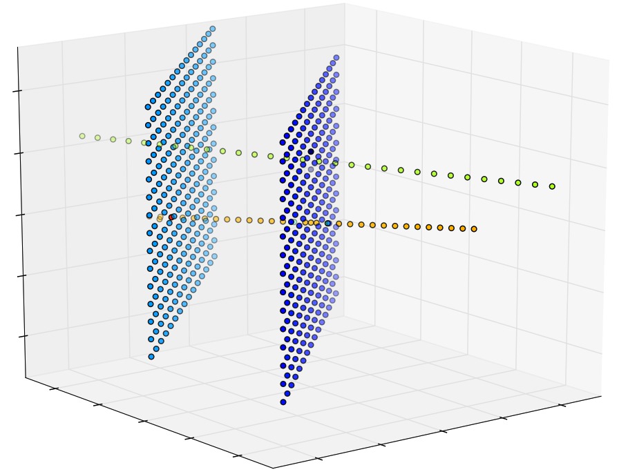
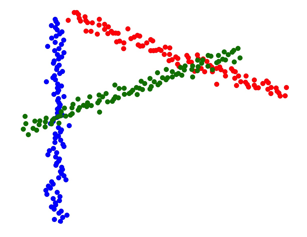
(a)	(b)	(c)

Figure 1: Examples of data clustered along intersecting manifolds.

The special case of affine linear subspaces, known as subspace clustering, has been addressed in the machine learning and computer vision literature by many authors using a variety of techniques (cf. [19, 20, 21, 22, 23, 24, 25, 26]). More general manifold clustering has been considered in [27, 28, 29, 12, 30, 13, 14, 15, 18, 31]. In our approach, we exploit the fact that localized covariance tensors encode rich information about the tangential structure of the submanifolds that underlie the data. Combined with information about the (relative) positions of the data points, they yield an effective data representation for manifold clustering. Although several different clustering techniques could be applied to the “tensorized” data, we use the single linkage hierarchical method because it produces provenly stable dendrograms. In conjunction with the stability and consistency results for covariance fields, this ensures that the manifold clustering method is stable at all steps. Dendrogram stability is analyzed in the framework of [32].

Contributions and Organization of the paper

The paper includes several illustrations and applications of CTFs to data analysis. For example, to illustrate how geometric information can be extracted from CTFs, we show that the curvature of plane curves and the principal curvatures of surfaces in $\mathbb{R}^{3}$ can be calculated from the spectrum of multiscale CTFs. Thus, multiscale covariance tensors give a way of extending these infinitesimal measures of geometric complexity to all scales and general probability distributions, not just those supported on smooth submanifolds. We also apply multiscale CTFs to manifold clustering, the problem of clustering Euclidean data that are organized along a finite union of possibly intersecting smooth submanifolds. Fig. 1 shows three such examples.

The main goals of the paper are: (i) to establish the foundations for analysis, visualization and management of data with methods based on multiscale covariance tensor fields, and (ii) to describe applications that characterize the usefulness of CTFs in data analysis. In Section 2, we formulate the notion of multiscale CTFs for a broad class of kernels and give examples that illustrate how CTFs reveal the geometry of data. In Section 3, we show that the curvature of a plane curve and the principal curvatures of a surface in $\mathbb{R}^{3}$ can be recovered from small-scale covariance. Section 4 is devoted to the main theoretical developments. We prove stability and consistency theorems for multiscale covariance tensor fields under mild regularity assumptions on the kernel, and also analyze rates of convergence that are important for applications in data analysis. Since some discontinuous kernels are of practical interest, we also investigate convergence results for such kernels, including a pointwise central limit theorem. Multiscale Fréchet functions are discussed in Section 5 and manifold clustering in Section 6. We close with a summary and some discussion.

2 Covariance Tensor Fields

2.1 Preliminaries

To define covariance tensor fields, we introduce some notation. Elements of the tensor product $\mathbb{R}^{d}\otimes\mathbb{R}^{d}$ may be identified with bilinear forms $B\colon\mathbb{R}^{d}\times\mathbb{R}^{d}\to\mathbb{R}$ through the Euclidean inner product. More precisely, a pure tensor $x\otimes y$ corresponds to the bilinear form

$$x\otimes y\,(u,v)=\left\langle x,u\right\rangle\cdot\left\langle y,v\right\rangle,$$ (1)

$\forall u,v\in\mathbb{R}^{d}$, where $\left\langle\,,\right\rangle$ denotes Euclidean inner product. Bilinear forms associated with more general elements of $\mathbb{R}^{d}\otimes\mathbb{R}^{d}$ can be described by linear extension. In Euclidean coordinates, we abuse notation and also write the coordinate vectors of $x,y\in\mathbb{R}^{d}$ as $x$ and $y$. With this convention, letting $A$ be the $d\times d$ matrix $A=xy^{T}$, we have

$$x\otimes y\,(u,v)=\left\langle u,Av\right\rangle,$$ (2)

where the superscript $T$ denotes transposition. In this manner, using Euclidean coordinates, an element of $\mathbb{R}^{d}\otimes\mathbb{R}^{d}$ also can be identified with a $d\times d$ matrix by linear extension of the correspondence $x\otimes y\leftrightarrow A$. Through these identifications, we refer to an element $\Sigma\in\mathbb{R}^{d}\otimes\mathbb{R}^{d}$ interchangeably as a tensor, a bilinear form or a matrix. We equip $\mathbb{R}^{d}\otimes\mathbb{R}^{d}$ with the inner product defined on pure tensors by

$$\left\langle x_{1}\otimes y_{1},x_{2}\otimes y_{2}\right\rangle=\left\langle x_{1},x_{2}\right\rangle\left\langle y_{1},y_{2}\right\rangle$$ (3)

and extended linearly to $\mathbb{R}^{d}\otimes\mathbb{R}^{d}$. Thus, the corresponding norm satisfies

$$\|x\otimes y\|=\|x\|\|y\|\,,$$ (4)

for any $x,y\in\mathbb{R}^{d}$. In matrix representation, this is the Frobenius norm.

Throughout the paper, we view $\mathbb{R}^{d}$ as a measurable space equipped with the Borel $\sigma$-algebra for the Euclidean metric. Let $y$ be an $\mathbb{R}^{d}$-valued random variable distributed according to the probability measure $\alpha$. Suppose that $y$ has expected value $\mathbb{E}\left[y\right]=\mu\in\mathbb{R}^{d}$ and finite second moment. As a motivation for the definition of multiscale CTFs, recall that the covariance tensor of $y$ is defined as

$$\Sigma_{\alpha}(\mu)=\mathbb{E}\left[(y-\mu)\otimes(y-\mu)\right]=\int_{\mathbb{R}^{d}}(y-\mu)\otimes(y-\mu)\,\alpha(dy)\in\mathbb{R}^{d}\otimes\mathbb{R}^{d}\,.$$ (5)

In matrix notation,

$$\Sigma_{\alpha}(\mu)=\int_{\mathbb{R}^{d}}(y-\mu)(y-\mu)^{T}\,\alpha(dy)\,.$$ (6)

The bilinear form associated with $\Sigma_{\alpha}(\mu)$ clearly is symmetric and positive semi-definite.

Covariation of $y$ may be measured with respect to any $x\in\mathbb{R}^{d}$, not just $\mu$. Thus, $\Sigma_{\alpha}(\mu)$ may be extended to a global covariance tensor field $\Sigma_{\alpha}\colon\mathbb{R}^{d}\to\mathbb{R}^{d}\otimes\mathbb{R}^{d}$ given by

$$\Sigma_{\alpha}(x)=\int_{\mathbb{R}^{d}}(y-x)\otimes(y-x)\,\alpha(dy)\,.$$ (7)

Note, however, that

$$\Sigma_{\alpha}(x)=\Sigma_{\alpha}(\mu)+(\mu-x)\otimes(\mu-x)\,,$$ (8)

for any $x\in\mathbb{R}^{d}$. Thus, for $x\neq\mu$, $\Sigma_{\alpha}(x)$ does not reveal any information about the distribution of $y$ other than that already contained in $\Sigma_{\alpha}(\mu)$. In contrast, as we shall see below, multiscale analogues are rich in information about the shape of $\alpha$.

2.2 Multiscale Covariance Tensor Fields

We adopt the notation $d$ for the volume of the unit ball in $\mathbb{R}^{d}$ and $\omega_{d-1}$ for the “surface area” of the unit sphere $\mathbb{S}^{d-1}\subset\mathbb{R}^{d}$, $d\geq 1$. Recall that $\omega_{d-1}=2\pi^{d/2}/\Gamma(d/2)$, where $\Gamma(\cdot)$ is the Gamma function, and $\omega_{d-1}=d\,d$. We make the convention that $0=1$.

Let $y$ be an $\mathbb{R}^{d}$-valued random variable with distribution $\alpha$ and let $K$ be a multiscale kernel; that is, a measurable function $K:\mathbb{R}^{d}\times\mathbb{R}^{d}\times(0,\infty)\to\mathbb{R}$ such that $K(x,y,\sigma)\geqslant 0$, for any $x,y\in\mathbb{R}^{d}$ and $\sigma>0$.

Definition 1.

The multiscale covariance tensor field (CTF) of $y$ associated with the kernel $K$ is the one-parameter family of tensor fields, indexed by $\sigma\in(0,\infty)$, given by

$$\Sigma_{\alpha}(x,\sigma):=\int_{\mathbb{R}^{d}}(y-x)\otimes(y-x)K(x,y,\sigma)\,\alpha(dy)\,,$$ (9)

provided that the integral converges for each $x\in\mathbb{R}^{d}$ and $\sigma>0$.

Remark 1.

Note that $\Sigma_{\alpha}$ depends only on the probability measure $\alpha$, not on $y$. For this reason, we refer to $\Sigma_{\alpha}$ interchangeably as the multiscale CTF of the random variable $y$ or the probability measure $\alpha$.

$\Sigma_{\alpha}(x,\sigma)$ measures the covariation of $y$ about $x$ with probability mass at $y$ weighted by $K(x,y,\sigma)$. It is simple to verify that the bilinear form $\Sigma_{\alpha}(x,\sigma)$ is symmetric and positive semi-definite. Note that if $K$ is bounded for each $\sigma>0$, that is, $\exists M_{\sigma}>0$ such that $K(x,y,\sigma)\leq M_{\sigma}$, $\forall x,y\in\mathbb{R}^{d}$, then $\Sigma_{\alpha}(x,\sigma)$ is well defined for any random variable $y$ with finite second moment. In particular if $K\equiv 1$, $\Sigma_{\alpha}(x,\sigma)=\Sigma_{\alpha}(x)$, $\forall x\in\mathbb{R}^{d}$. However, as our primary goal is to study the organization of data and random variables at scales ranging from local to global, we consider kernels in $\mathbb{R}^{d}$ that satisfy additional decay conditions as they produce a windowing effect. The kernels are constructed as follows.

Definition 2.

Let $d$ be a positive integer and $f\colon[0,\infty)\to\mathbb{R}$ a bounded and measurable function satisfying:

• $f(r)\geqslant 0$, $\forall r\in[0,\infty)$;

• $M_{d}=\int_{0}^{\infty}r^{\frac{d}{2}-1}f(r)\,dr<\infty$;

• There is $C>0$ such that $rf(r)\leq C$, $\forall r\in[0,\infty)$.

The multiscale kernel $K\colon\mathbb{R}^{d}\times\mathbb{R}^{d}\times(0,\infty)\to\mathbb{R}$ associated with $f$ is defined as

$$K(x,y,\sigma):=\frac{1}{C_{d}(\sigma)}\,f\left(\frac{\|y-x\|^{2}}{\sigma^{2}}\right),$$ (10)

where $C_{d}(\sigma)=\frac{1}{2}\sigma^{d}M_{d}\,\omega_{d-1}$.

Condition (b) in the definition implies that the normalizing constant $C_{d}(\sigma)$ is well defined. The normalization is adopted so that $\int K(x,y,\sigma)\,dy=1$, $\forall x\in\mathbb{R}^{d}$ and $\forall\sigma>0$. Condition (c) guarantees that the integral in (9) is convergent for any probability measure $\alpha$. Henceforth, for convenience, we assume that $\sup f=1$. This is not restrictive since scaling $f$ does not change the kernel $K$ because of the normalization.

Whereas we investigate properties of multiscale CTFs in a more general setting, our examples and experiments focus on two special kernels:

• The isotropic Gaussian kernel

  $$G(x,y,\sigma)=\frac{1}{(2\pi\sigma^{2})^{d/2}}\exp\left(-\frac{\|y-x\|^{2}}{2\sigma^{2}}\right),$$ (11)

  which is associated with the function $f(x)=e^{-x/2}$;

• The truncation kernel

  $$T(x,y,\sigma)=\frac{1}{\sigma^{d}d}\,\chi\left(\frac{\|y-x\|^{2}}{\sigma^{2}}\right)$$ (12)

  associated with the characteristic function $\chi\colon[0,\infty)\to\mathbb{R}$ of the unit interval $\left[0,1\right]$. In measuring covariation of random variables about $x$, the kernel $T$ attributes a uniform weight to mass at points within the closed ball of radius $\sigma$ centered at $x$ and weight zero to mass elsewhere.

Remark 2.

The kernel $K$ defined in (10) is homogeneous and isotropic; that is, for any isometry $\varphi\colon\mathbb{R}^{d}\to\mathbb{R}^{d}$, $K(\varphi(x),\varphi(y),\sigma)=K(x,y,\sigma)$, $\forall x,y\in\mathbb{R}^{d}$ and $\sigma>0$. Moreover, if we write $\varphi(x)=Ux+b$, with $U\in O(d)$ and $b\in\mathbb{R}^{d}$, then

$$U\,\Sigma_{\alpha}(x,\sigma)\,U^{T}=\Sigma_{\varphi_{\ast}(\alpha)}(\varphi(x),\sigma),$$ (13)

for any $(x,\sigma)\in\mathbb{R}^{d}\times(0,\infty)$. Here $O(d)$ is the group of $d\times d$ orthogonal matrices and $\varphi_{\ast}(\alpha)$ is the pushforward of $\alpha$ under $\varphi$.

Remark 3.

Multiscale covariance tensor fields can be defined for any positive Borel measure $\alpha$ that satisfies

$$\int_{\mathbb{R}^{d}}\|z\|^{2}f(\|z\|^{2})\,\alpha(dz)<\infty\,,$$ (14)

not just for probability measures. In particular, if $f$ has compact support, covariance fields are defined for any locally finite Borel measure $\alpha$; that is, measures for which every point $p\in\mathbb{R}^{d}$ has an open neighborhood $U_{p}$ such that $\alpha(U_{p})<\infty$.

We conclude this section with examples that support our contention that multiscale covariance tensor fields are rich in information about the shape of data.

Example 1.

This example shows that the spectrum of multiscale covariance tensors allow us to estimate the dimensionality of data in a scale dependent manner. We consider the data points $y_{1},\ldots,y_{n}$ in $\mathbb{R}^{2}$, shown in Figure 2, and calculate $\Sigma_{\alpha_{n}}$ centered at one of the data points for the Gaussian kernel at scales $\sigma=0.1$ and $\sigma=2$. Here $\alpha_{n}$ denotes the empirical measure $n^{-1}\sum_{i=1}^{n}\delta_{y_{i}}$. The covariance tensors are depicted as ellipses whose principal axes are in the direction of the eigenvectors of the covariance matrix and principal radii are proportional to $\sqrt{\lambda_{1}}$ and $\sqrt{\lambda_{2}}$, where $0\leq\lambda_{1}\leq\lambda_{2}$ are the eigenvalues of the covariance. At scale $\sigma=0.1$, $\lambda_{1}/\lambda_{2}=0.908$, showing that the covariance tensor is nearly isotropic, indicating that the “dimension” of the data is 2. At $\sigma=2$, the ratio of the eigenvalues is $0.025$, giving a highly anisotropic covariance tensor, from which we infer that the dimension is 1.

$\sigma=0.1$	$\sigma=2$

Figure 2: Estimating data dimensionality at different scales through multiscale covariance.

Example 2 (A linear subspace of $\mathbb{R}^{d}$).

Let $v_{1},\ldots,v_{r}\in\mathbb{R}^{d}$, $1\leq r\leq d$, be orthonormal vectors and consider the subspace $H=<v_{1},\ldots,v_{r}>$ that they span. Let $\alpha$ denote the singular measure supported on $H$ induced by the volume form on $H$. The measure $\alpha$ clearly is locally finite. We calculate multiscale covariance fields at points $x\in H$ to show that $H$ may be recovered from $\Sigma_{\alpha}(x,\sigma)$. By Remark 2, we may assume that $x=0$. A calculation shows that for the Gaussian kernel,

$$\Sigma_{\alpha}(0,\sigma)=\frac{r}{(\sqrt{2\pi})^{d-r}\sigma^{d-r-2}}\sum_{i=1}^{r}\,v_{i}\otimes v_{i}\,.$$ (15)

For the truncation kernel,

$$\Sigma_{\alpha}(0,\sigma)=\lambda_{r}\sum_{i=1}^{r}\,v_{i}\otimes v_{i}\,,$$ (16)

where

$$\lambda_{r}=\frac{1}{\sigma^{d-r-2}}\frac{{r-1}}{d}\int_{-\pi/2}^{\pi/2}\sin^{2}\theta\cos^{r}\theta\,d\theta\,.$$ (17)

For $r=1$, this expression simplifies to $\lambda_{1}=2/(3\sigma^{d-3}d)$. Thus, for both kernels, the orthogonal complement of $H$ is the null space of $\Sigma_{\alpha}(0,\sigma)$ and $H$ is the eigenspace associated with the positive eigenvalue $\lambda_{r}$.

Example 3 (Wedge of $n$ segments).

Consider the wedge (one-point union) $W$ of $n$ segments $L_{1},\ldots,L_{n}$ in $\mathbb{R}^{d}$ attached at the origin, as depicted in Fig. 3. Each segment $L_{i}$ is determined by its length $\ell_{i}>0$ and a unit direction vector $v_{i}$. We assume that $v_{i}\neq v_{j}$, for any $1\leq i<j\leq n$. Let $\alpha$ be the singular measure on $\mathbb{R}^{d}$ that is supported on $W$ and agrees with the measure induced by arc length on each segment $L_{i}$. We consider the multiscale covariance field of $\alpha$ associated with the truncation kernel. For $x\in L_{i}$, $x\neq 0$, as in the case $r=1$ in Example 2, we have that $\Sigma_{\alpha}(x,\sigma)=(2/3\sigma^{d-3}d)\,v_{i}\otimes v_{i}$ at small enough scales. Thus, $\Sigma_{\alpha}(x,\sigma)$ has rank one. However, at the origin,

$$\Sigma_{\alpha}(0,\sigma)=\frac{1}{3\sigma^{d}d}\sum_{i=1}^{n}\left(\min(\sigma,\ell_{i})\right)^{3}v_{i}\otimes v_{i}\,.$$ (18)

for any $\sigma>0$. Thus, for $\sigma\leq\min\{\ell_{i},1\leq i\leq n\}$,

$$\Sigma_{\alpha}(0,\sigma)=\frac{1}{3\sigma^{d-3}d}\sum_{i=1}^{n}v_{i}\otimes v_{i}\,.$$ (19)

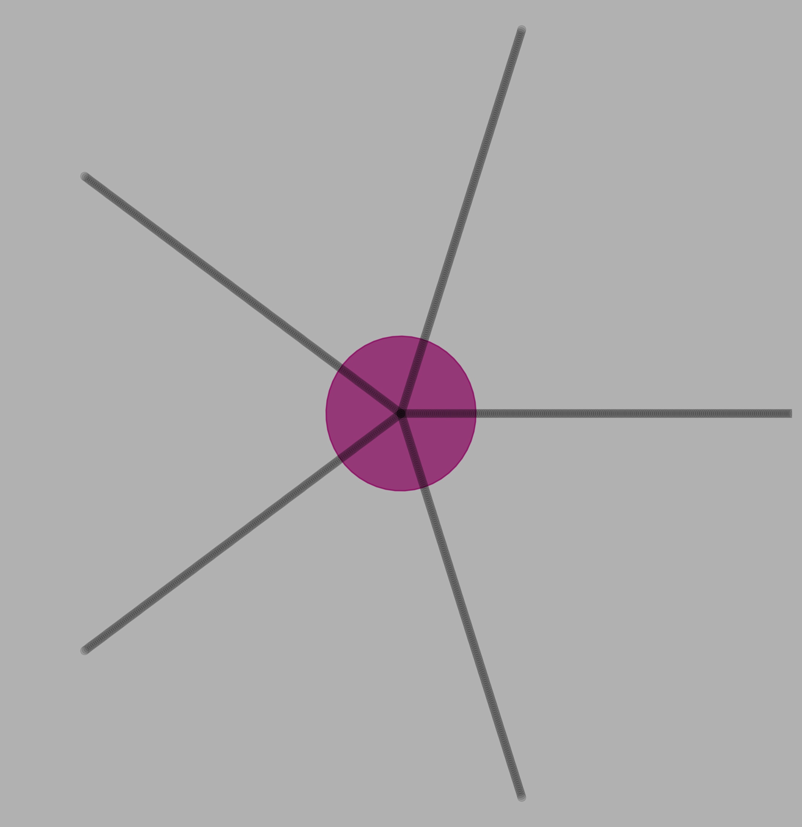
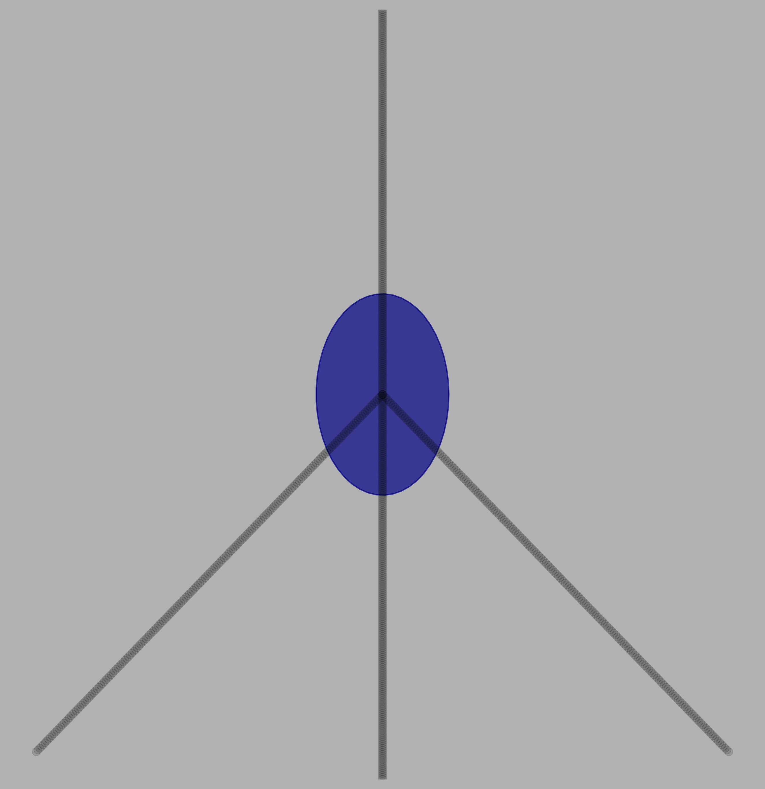
Figure 3: Covariance at the one-point union of line segments.

3 Geometry of Curves and Surfaces

In this section, we show how multiscale CTFs associated with the truncation kernel extract precise local geometric information from plane curves and surfaces in $\mathbb{R}^{3}$.

3.1 Plane Curves

Example 4.

We begin with the special case of a circle. Let $C_{R}\subset\mathbb{R}^{2}$ be the circle of radius $R$ centered at the origin in $\mathbb{R}^{2}$ and $\alpha$ the singular measure supported on $C_{R}$ induced by arc length. For any $x\in\mathbb{R}^{2}$, we denote $r=\|x\|$. If $x$ is such that $\left|r-R\right|>\sigma$ then ${\Sigma}_{\alpha}(x,\sigma)=0.$ Assume that $x\in\mathbb{R}^{2}$ and $0<\sigma<R$ are such that $r\in[R-\sigma,R+\sigma]$. In this case, in the coordinate system given by the directions $n=x/\|x\|$ and $t=n^{\perp}$, a calculation shows that $\Sigma_{\alpha}(x,\sigma)$ is diagonal with entries

$$\begin{split}\lambda_{n}(x,\sigma)&=\frac{1}{\pi\sigma^{2}}\left[R{\phi\left(R^{2}+2r^{2}\right)+R^{2}(R\cos\phi-4r)\sin\phi}\right]\\ \lambda_{t}(x,\sigma)&={\frac{R^{3}}{\pi\sigma^{2}}(\phi-\sin\phi\cos\phi)}\,,\end{split}$$ (20)

where $\phi=\arccos\left(\frac{R^{2}+r^{2}-\sigma^{2}}{2rR}\right)$. Thus, the normal and tangential vectors, $n$ and $t$, are eigenvectors with eigenvalues $\lambda_{n}$ and $\lambda_{t}$, respectively. Fig. 4 shows the eigenvalues as functions of $r$, $0.9\leq r\leq 1.1$, for $\sigma=0.1$.

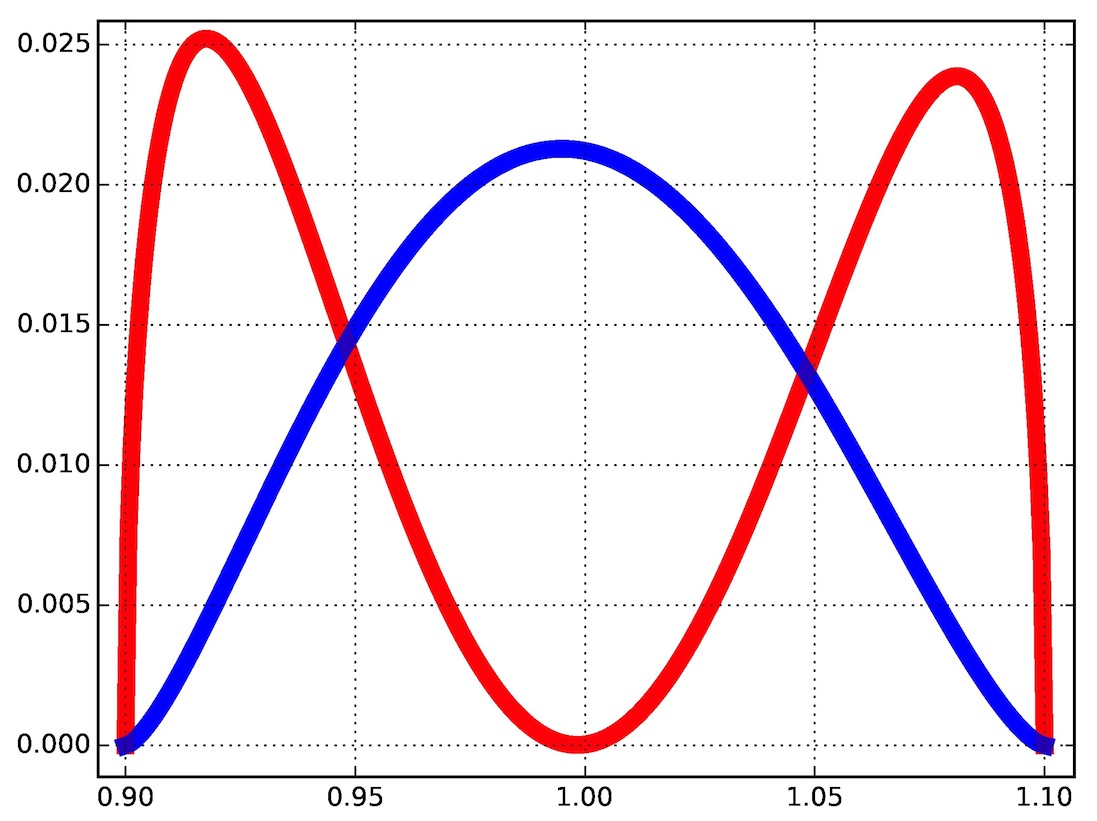
Figure 4: Tangential (blue) and normal (red) eigenvalues as a function of $r$, $0.9\leq r\leq 1.1$, at $\sigma=0.1$, of the multiscale CTF associated with the truncation kernel for the singular measure induced by arc length, supported on the unit circle in $\mathbb{R}^{2}$.

Now we consider a general smooth curve $C\subset\mathbb{R}^{2}$, that is, a 1-dimensional, smooth, properly embedded submanifold of $\mathbb{R}^{2}$. Let $\alpha$ be the singular measure on $\mathbb{R}^{2}$ supported on $C$ and induced by arc length. This measure is locally finite because the embedding is proper. We calculate the small-scale covariance at points on $C$ for the truncation kernel and show that the curvature can be recovered from the eigenvalues of $\Sigma_{\alpha}$. Let $x\in C$ be fixed. The arc-length parametrization of $C$ near $x$ may be written as

$$X(s)=s-\frac{\kappa^{2}s^{3}}{6}+O(s^{4})\quad\text{and}\quad Y(s)=\frac{\kappa s^{2}}{2}+\frac{\kappa_{s}s^{3}}{6}+O(s^{4})\,,$$ (21)

where $X(s)$ and $Y(s)$ are coordinates along the tangent and normal to $C$ at $x$, respectively [33]. Here, the curvature $\kappa$ and its derivative $\kappa_{s}$ are evaluated at $x$. A calculation yields:

Proposition 1.

Let $\sigma>0$ be small. If $C$ is a smooth plane curve and $x\in C$, then in the coordinates specified above we have

$${\Sigma}_{\alpha}(x,\sigma)=\left(\begin{matrix}\frac{2\sigma}{3\pi}-\frac{\kappa^{2}\sigma^{3}}{20\pi}+O(\sigma^{4})\quad&\frac{\kappa_{s}\sigma^{3}}{15\pi}+O(\sigma^{4})\\ \frac{\kappa_{s}\sigma^{3}}{15\pi}+O(\sigma^{4})&\frac{\kappa^{2}\sigma^{3}}{10\pi}+O(\sigma^{4})\end{matrix}\right).$$ (22)

Proposition 1 implies that, for $\sigma>0$ small, the eigenvalues of $\Sigma_{\alpha}$ are

$$\lambda_{1}=\frac{2\sigma}{3\pi}-\frac{\kappa^{2}\sigma^{3}}{20\pi}+O(\sigma^{4})\quad\text{and}\quad\lambda_{2}=\frac{\kappa^{2}\sigma^{3}}{10\pi}+O(\sigma^{4})\,,$$ (23)

so that

$$\text{tr}\,\Sigma_{\alpha}(x,\sigma)=\frac{2\sigma}{3\pi}+\frac{\kappa^{2}\sigma^{3}}{20\pi}+O(\sigma^{4})\,.$$ (24)

Thus, the curvature at $x\in C$ may be recovered, up to a sign, as

$$\kappa=\pm\lim_{\sigma\to 0}\frac{\sqrt{20\pi}}{\sigma^{3/2}}\left(\text{tr}\,\Sigma_{\alpha}(x,\sigma)-\frac{2\sigma}{3\pi}\right)^{1/2}.$$ (25)

3.2 Surfaces in $\mathbb{R}^{3}$

Example 5.

Let $S_{R}$ be the sphere of radius $R$ centered at the origin in $\mathbb{R}^{3}$. For $x\in\mathbb{R}^{3}$, we let $r=\|x\|$. If $x$ is such that $\left|r-R\right|>\sigma$, then ${\Sigma_{\alpha}}(x,\sigma)=0.$ Assume that $x\neq(0,0,0)$ and $\sigma>0$ are such that $r\in[R-\sigma,R+\sigma]$. In the coordinate system given by the vector $n=x/\|x\|$, and any orthonormal basis $\{t_{1},t_{2}\}$ of the orthogonal complement $n^{\perp}$, a direct calculation shows that ${\Sigma_{\alpha}}(x,\sigma)$ is a $3\times 3$ diagonal matrix with entries

$$\begin{split}\lambda_{t_{1}}(x,\sigma)&=\lambda_{t_{2}}(x,\sigma)=\frac{R^{4}}{\sigma^{3}}\sin^{4}\left(\frac{\phi}{2}\right)(\cos\phi+2)\\ \lambda_{n}(x,\sigma)&=\frac{R^{2}}{2\sigma^{3}}(1-\cos\phi)\left(R^{2}+R\cos\phi(R\cos\phi+R-3r)\right)\\ &+\frac{R^{2}}{2\sigma^{3}}(1-\cos\phi)\left(-3Rr+3r^{2}\right)\end{split}$$ (26)

where $\phi=\arccos\left(\frac{R^{2}+r^{2}-\sigma^{2}}{2Rr}\right)$. In particular, this means that $\lambda_{n}$ is the eingenvalue corresponding to the eigenvector $n$ along the normal direction to the sphere at $x/\|x\|$, and $\{t_{1},t_{2}\}$ span the eigenspace along the tangent directions with eigenvalue $\lambda_{t_{1}}=\lambda_{t_{2}}$. Fig. 5 shows a plot of the eigenvalues as a function of $r$, $0.9\leq r\leq 1,1$, for $\sigma=0.1$.

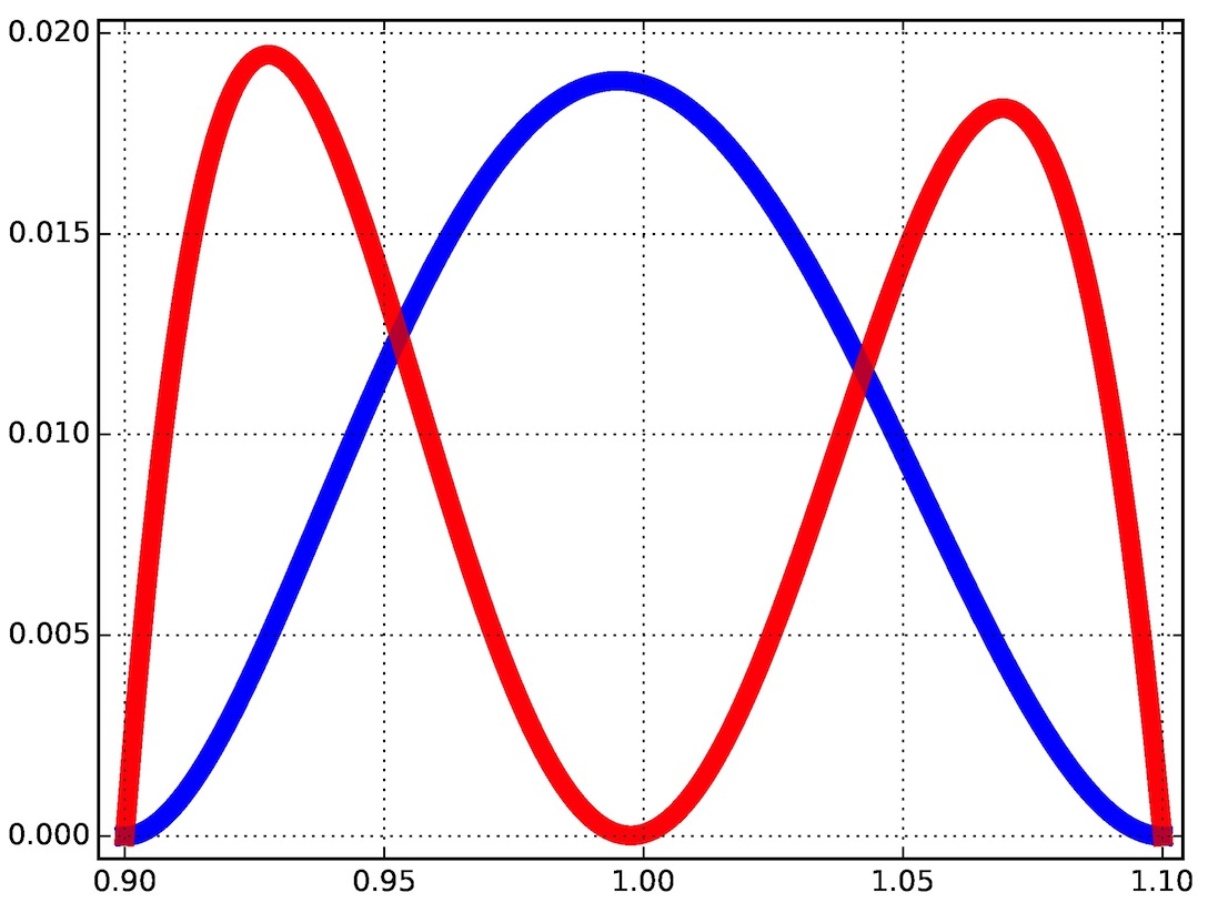
Figure 5: Tangential (blue) and normal eigenvalues (red) of the multiscale CTF associated with the truncation kernel as a function of $r$, $0.9\leq r\leq 1.1$, at $\sigma=0.1$, for the singular measure induced by surface area, supported on the unit sphere in $\mathbb{R}^{3}$.

Now we consider a general smooth compact surface $S\subset\mathbb{R}^{3}$. Let $\alpha$ be the singular measure on $\mathbb{R}^{3}$ supported on $S$ and induced by the area measure on $S$. We calculate the small-scale covariance at points on $S$ for the truncation kernel and show that the principal curvatures may indeed be recovered from the spectrum of ${\Sigma}$. Given a non-umbilic point $p\in S$, one can choose a Cartesian coordinate system centered at $p$ so that the $x$-axis is along the direction of maximal curvature at $p$, the $y$-axis is along the direction of minimal curvature at $p$, and the $z$-axis is along the normal to $S$ at $p$.

Proposition 2.

Let $\sigma>0$ be small, $p\in S$ be non-umbilic, and $\alpha$ be the surface area measure on $S$. In the coordinate system described above, the covariance tensor for the truncation kernel is given by

$$\Sigma_{\alpha}(p,\sigma)=\begin{bmatrix}A_{t_{1}}&O(\sigma^{4})&O(\sigma^{5})\\ O(\sigma^{4})&A_{t_{2}}&O(\sigma^{5})\\ O(\sigma^{5})&O(\sigma^{5})&A_{n}\end{bmatrix},$$ (27)

where

$$\begin{split}A_{t_{1}}&=\frac{3\sigma}{16}+\frac{1}{256}(-3\kappa_{1}^{2}-6\kappa_{1}\kappa_{2}+\kappa_{2}^{2})\sigma^{3}+O(\sigma^{4}),\\ A_{t_{2}}&=\frac{3\sigma}{16}+\frac{1}{256}(\kappa_{1}^{2}-6\kappa_{1}\kappa_{2}-3\kappa_{2}^{2})\sigma^{3}+O(\sigma^{4}),\\ A_{n}&=\frac{3\kappa_{1}^{2}+2\kappa_{1}\kappa_{2}+3\kappa_{2}^{2}}{128}\sigma^{3}+O(\sigma^{4}),\end{split}$$ (28)

and $\kappa_{1}>\kappa_{2}$ are the principal curvatures of $S$ at $p$.

It follows from this result that, for $\sigma>0$ small,

$$\begin{split}\text{tr}\,\Sigma_{\alpha}(p,\sigma)&=\frac{3}{16}\sigma+\frac{1}{64}(\kappa_{1}-\kappa_{2})^{2}\sigma^{3}+O(\sigma^{4})\ \text{and}\\ \text{det}\,\Sigma_{\alpha}(p,\sigma)&=\big{(}{3\kappa_{1}^{2}+2\kappa_{1}\kappa_{2}+3\kappa_{2}^{2}\big{)}}\frac{\pi^{2}}{2048}\sigma^{11}+O(\sigma^{12})\,.\end{split}$$ (29)

As a consequence, $\kappa_{1}$ and $\kappa_{2}$ can be recovered from the spectrum of ${\Sigma}_{\alpha}(p,\sigma)$ as a function of $\sigma$. Indeed, from the small scale asymptotics of the trace and determinant of $\Sigma_{\alpha}(p,\sigma)$, we can extract the values of $(\kappa_{1}-\kappa_{2})^{2}$ and $3\kappa_{1}^{2}+2\kappa_{1}\kappa_{2}+3\kappa_{2}^{2}$ from which we can determine the values of $\kappa_{1}$ and $\kappa_{2}$.

Proof of Proposition 2.

Using cylindrical coordinates in the chosen reference system, we can parametrize the patch $S\cap B(p,\sigma)$ as $(\rho\cos\phi,\rho\sin\phi,z(\rho,\phi))$, for $\phi\in[0,2\pi]$, $\rho\in[0,\rho_{\sigma}(\phi)]$, where $\rho_{\sigma}(\phi)=\sigma-\frac{1}{8}\big{(}\kappa_{1}(\cos\phi)^{2}+\kappa_{2}(\sin\phi)^{2}\big{)}^{2}\sigma^{3}+O(\sigma^{4})$, and $z(\rho,\phi)=\frac{\rho^{2}}{2}\big{(}\kappa_{1}(\cos\phi)^{2}+\kappa_{2}(\sin\phi)^{2}\big{)}+O(\sigma^{3}).$ The area element on the patch is given by

$$dA=\left(\rho+\frac{\rho^{3}}{2}(\kappa_{1}^{2}(\cos\phi)^{2}+\kappa_{2}^{2}(\sin\phi)^{2})+O(\rho^{5})\right)d\rho\,d\phi.$$ (30)

Now we have all the ingredients needed to compute $\Sigma_{\alpha}(p,\sigma)$. For example, to calculate the $(1,1)$-entry, we express $\iint_{S\cap B(0,\sigma)}x^{2}\,dA$ as

$$\int_{0}^{2\pi}\int_{0}^{\rho_{\sigma}(\phi)}\left[\rho^{3}\cos^{2}\phi+\frac{\rho^{5}\cos^{2}\phi}{2}\left(\kappa_{2}^{2}\sin^{2}\phi+\kappa_{1}^{2}\cos^{2}\phi\right)+O(\rho^{6})\right]d\rho\,d\phi\,,$$ (31)

which after a simple but tedious calculation yields the desired result. The computation of other entries of the matrix follows similar steps. ∎

4 Stability and Consistency

For each $p\in[1,\infty)$, let $\mathcal{P}_{p}(\mathbb{R}^{d})$ denote the collection of all Borel probability measures $\alpha$ on $\mathbb{R}^{d}$ whose $p$th moment $M_{p}(\alpha)=\int\|z\|^{p}\alpha(dz)$ is finite. We adopt the notation $m_{p}(\alpha)=M^{1/p}_{p}(\alpha)$. For $p=\infty$, we let $\mathcal{P}_{\infty}(\mathbb{R}^{d})$ be the collection of all Borel probability measures on $\mathbb{R}^{d}$ with bounded support and $m_{\infty}(\alpha)=\sup\{\|z\|,\,z\in\mathrm{supp}\,[\alpha]\}$. By Jensen’s inequality, if $1\leq q\leq p\leq\infty$, then $\mathcal{P}_{p}(\mathbb{R}^{d})\subset\mathcal{P}_{q}(\mathbb{R}^{d})$ and $m_{q}(\alpha)\leq m_{p}(\alpha)$, for any $\alpha\in\mathcal{P}_{p}(\mathbb{R}^{d})$.

Definition 3.

For $p\in[1,\infty]$ and $\lambda>0$, we define $\mathcal{P}_{p}^{\lambda}(\mathbb{R}^{d})\subset\mathcal{P}_{p}(\mathbb{R}^{d})$ as the subset of all $\alpha\in\mathcal{P}_{p}(\mathbb{R}^{d})$ such that $\alpha(A)\leq\lambda\,\mathcal{L}(A)$, for all measurable sets $A$, where $\mathcal{L}$ stands for Lebesgue measure.

Example 6.

If $\alpha\in\mathcal{P}_{p}(\mathbb{R}^{d})$ is absolutely continuous with respect to the Lebesgue measure with density function $f\in\mathbb{L}^{\infty}(\mathbb{R}^{d})$ satisfying $\|f\|_{\infty}\leq\lambda$, then $\alpha\in\mathcal{P}_{p}^{\lambda}(\mathbb{R}^{d})$.

Let us recall the definition of the $p$-Wasserstein distance $W_{p}(\alpha,\beta)$ between $\alpha,\beta\in\mathcal{P}_{p}(\mathbb{R}^{d})$. Let $\Gamma(\alpha,\beta)$ be the collection of all couplings of $\alpha$ and $\beta$; that is, probability measures $\mu$ on $\mathbb{R}^{d}\times\mathbb{R}^{d}$ such that $(\pi_{1})_{\ast}\mu=\alpha$ and $(\pi_{2})_{\ast}\mu=\beta$, where $\pi_{1},\pi_{2}\colon\mathbb{R}^{d}\times\mathbb{R}^{d}\to\mathbb{R}^{d}$ denote projections onto the first and second components, respectively.

Definition 4.

For $p\in[1,\infty)$, the $p$-Wasserstein distance between $\alpha,\beta\in\mathcal{P}_{p}(\mathbb{R}^{d})$ is given by

$$W_{p}(\alpha,\beta):=\inf_{\mu\in\Gamma(\alpha,\beta)}\left(\iint\|z_{1}-z_{2}\|^{p}\mu(dz_{1}\times dz_{2})\right)^{1/p},$$

and the $\infty$-Wasserstein distance between $\alpha,\beta\in\mathcal{P}_{\infty}(\mathbb{R}^{d})$ by

$$W_{\infty}(\alpha,\beta):=\inf_{\mu\in\Gamma(\alpha,\beta)}\sup\left\{\|z_{1}-z_{2}\|,\,(z_{1},z_{2})\in\mathrm{supp}\,[\mu]\right\}.$$

Remark 4.

• For any $\alpha,\beta\in\mathcal{P}_{p}(\mathbb{R}^{d})$, $p\in[1,\infty]$, there exists a coupling that realizes the infimum in the definition of $W_{p}(\alpha,\beta)$ (cf. [34]).

• It is a standard result that, for each $p\in[1,\infty)$, $W_{p}$ defines a metric on $\mathcal{P}_{p}(\mathbb{R}^{d})$ that is compatible with weak convergence of probability measures [3].

• If $\varphi\colon\mathbb{R}^{d}\to\mathbb{R}^{d}$ is an isometry, then $W_{p}(\alpha,\beta)=W_{p}(\varphi_{\ast}(\alpha),\varphi_{\ast}(\beta))$, for any $\alpha,\beta\in\mathcal{P}_{p}(\mathbb{R}^{d})$.

4.1 Smooth Kernels

Theorem 1 (Stability for Smooth Kernels).

Let $f\colon[0,\infty)\to\mathbb{R}$ be as in Definition 2 with multiscale kernel $K$. Suppose that $f$ is differentiable and there exists a constant $A_{1}>0$ such that $r^{3/2}\,|f^{\prime}(r)|\leq A_{1}$, $\forall r\geq 0$. Then, there is a constant $A_{f}>0$, that depends only on $f$, such that

$$\sup_{x\in\mathbb{R}^{d}}\left\|\Sigma_{\alpha}(x,\sigma)-\Sigma_{\beta}(x,\sigma)\right\|\leq\frac{\sigma A_{f}}{C_{d}(\sigma)}\,W_{1}(\alpha,\beta),$$

for any $\alpha,\beta\in\mathcal{P}_{1}(\mathbb{R}^{d})$ and any $\sigma>0$. Here $\|\cdot\|$ is the norm associated with the inner product defined in (3).

Theorem 1 shows that multiscale covariance fields yield a robust representation of probability measures that make their geometric properties more readily accessible, as illustrated in our examples. In Section 5, we show that not only is $\Sigma_{\alpha}(\cdot,\sigma)$ stable, but all the information contained in the probability measure $\alpha$ is fully absorbed into the multiscale CTF associated with the Gaussian kernel. In fact, $\alpha$ may be recovered from the multiscale scalar field given by $V_{\alpha}(x,\sigma)=\mathrm{tr}\,\Sigma_{\alpha}(x,\sigma)$, $x\in\mathbb{R}^{d}$ and $\sigma>0$.

The following lemma will be used in the proof of the stability theorem for smooth kernels. To simplify notation, we define $K_{\sigma}\colon\mathbb{R}^{d}\to\mathbb{R}$ by

$$K_{\sigma}(z)=K(z,0,\sigma)=\frac{1}{C_{d}(\sigma)}\,f\left(\frac{\|z\|^{2}}{\sigma^{2}}\right)$$ (32)

and $Q_{\sigma}\colon\mathbb{R}^{d}\to\mathbb{R}^{d}\otimes\mathbb{R}^{d}$ by

$$Q_{\sigma}(z)=(z\otimes z)K_{\sigma}(z)\,.$$ (33)

Lemma 1.

Let $f$ be as in Definition 2 and suppose that $f$ is differentiable and there is a constant $A_{1}>0$ such that $r^{3/2}\,|f^{\prime}(r)|\leq A_{1}$, $\forall r\geq 0$. Then, there is a constant $A_{f}>0$, that depends only on $f$, such that

$$\left\|Q_{\sigma}(z_{1})-Q_{\sigma}(z_{2})\right\|\leq\frac{A_{f}\sigma}{C_{d}(\sigma)}\|z_{1}-z_{2}\|,$$

for any $z_{1},z_{2}\in\mathbb{R}^{d}$ and all $\sigma>0$.

Proof.

Let $z(t)=tz_{1}+(1-t)z_{2}$, $0\leq t\leq 1$. Then,

$$\begin{split}Q_{\sigma}(z_{1})-Q_{\sigma}(z_{2})=\int_{0}^{1}\frac{d}{dt}Q_{\sigma}(z(t))\,dt\,.\end{split}$$ (34)

Since

$$\begin{split}\frac{d}{dt}Q_{\sigma}(z)&=\frac{(z_{1}-z_{2})\otimes z}{C_{d}(\sigma)}f\left(\frac{\|z\|^{2}}{\sigma^{2}}\right)+\frac{z\otimes(z_{1}-z_{2})}{C_{d}(\sigma)}f\left(\frac{\|z\|^{2}}{\sigma^{2}}\right)\\ &+(z\otimes z)\frac{2}{\sigma^{2}C_{d}(\sigma)}f^{\prime}\left(\frac{\|z\|^{2}}{\sigma^{2}}\right)\left(z\cdot(z_{1}-z_{2})\right)\,,\end{split}$$ (35)

it follows that

$$\begin{split}\left\|\frac{d}{dt}Q_{\sigma}(z)\right\|&\leq\frac{2\|z\|}{C_{d}(\sigma)}f\left(\frac{\|z\|^{2}}{\sigma^{2}}\right)\|z_{1}-z_{2}\|\\ &+\frac{2\|z\|^{3}}{\sigma^{2}C_{d}(\sigma)}\left|f^{\prime}\left(\frac{\|z\|^{2}}{\sigma^{2}}\right)\right|\|z_{1}-z_{2}\|\\ &=\frac{2\sigma}{C_{d}(\sigma)}\frac{\|z\|}{\sigma}f\left(\frac{\|z\|^{2}}{\sigma^{2}}\right)\|z_{1}-z_{2}\|\\ &+\frac{2\sigma}{C_{d}(\sigma)}\frac{\|z\|^{3}}{\sigma^{3}}\left|f^{\prime}\left(\frac{\|z\|^{2}}{\sigma^{2}}\right)\right|\|z_{1}-z_{2}\|\,.\end{split}$$ (36)

Since $f$ is smooth, condition (c) of Definition 2 ensures that there is a constant $A_{2}>0$ such that $\sqrt{r}f(r)\leq A_{2}$, $\forall r\geq 0$. Moreover, by hypothesis $r^{3/2}|f^{\prime}(r)|\leq A_{1}$. Thus, (36) implies that

$$\left\|\frac{d}{dt}Q_{\sigma}(z)\right\|\leq\frac{\sigma A_{f}}{C_{d}(\sigma)}\|z_{2}-z_{1}\|\,,$$ (37)

where $A_{f}=2(A_{1}+A_{2})$. The lemma follows from (34) and (37). ∎

Proof of Theorem 1.

Without loss of generality, we may assume that $x=0$. We express the covariance fields as

$$\Sigma_{\alpha}(x,\sigma)=\int Q_{\sigma}(z_{1})\,\alpha(dz_{1})\quad\text{and}\quad\Sigma_{\beta}(x,\sigma)=\int Q_{\sigma}(z_{2})\,\beta(dz_{2}).$$ (38)

Given $\eta>0$ satisfying $W_{1}(\alpha,\beta)<\eta$, let $\mu\in\Gamma(\alpha,\beta)$ be a coupling such that

$$\iint\|z_{1}-z_{2}\|\mu(dz_{1}\times dz_{2})<\eta\,.$$ (39)

We may write

$$\begin{split}\Sigma_{\alpha}(x,\sigma)=\int Q_{\sigma}(z_{1})\,\mu(dz_{1}\times dz_{2})\ \ \text{and}\ \ \Sigma_{\beta}(x,\sigma)=\int Q_{\sigma}(z_{2})\,\mu(dz_{1}\times dz_{2})\,.\end{split}$$ (40)

Therefore,

$$\left\|\Sigma_{\alpha}(x,\sigma)-\Sigma_{\beta}(x,\sigma)\right\|\leq\iint\|Q_{\sigma}(z_{1})-Q_{\sigma}(z_{2})\|\,\mu(dz_{1}\times dz_{2})\,.$$ (41)

Lemma 1 and (41) imply that

$$\begin{split}\left\|\Sigma_{\alpha}(x,\sigma)-\Sigma_{\beta}(x,\sigma)\right\|&\leq\frac{\sigma A_{f}}{C_{d}(\sigma)}\iint\|z_{1}-z_{2}\|\,\mu(dz_{1}\times dz_{2})\\ &\leq\frac{\sigma A_{f}}{C_{d}(\sigma)}\eta\,.\end{split}$$ (42)

Since (42) holds for any $\eta>W_{1}(\alpha,\beta)$, we can conclude that

$$\left\|\Sigma_{\alpha}(x,\sigma)-\Sigma_{\beta}(x,\sigma)\right\|\leq\frac{\sigma A_{f}}{C_{d}(\sigma)}W_{1}(\alpha,\beta)\,,$$ (43)

as claimed. ∎

In what follows, given random vectors $y_{i}\in\mathbb{R}^{d}$, $i\in\mathbb{N}$, we let $\alpha_{n}=\sum_{i=1}^{n}\delta_{y_{i}}/n$.

Corollary 1 (Consistency for Smooth Kernels).

Let $K$ be a multiscale kernel as in Theorem 1 and $\sigma>0$. If $\alpha\in\mathcal{P}_{1}(\mathbb{R}^{d})$ and $y_{i}\in\mathbb{R}^{d}$, $i\in\mathbb{N}$, are i.i.d. random variables with distribution $\alpha$, then

$$\sup_{x\in\mathbb{R}^{d}}\left\|\Sigma_{\alpha_{n}}(x,\sigma)-\Sigma_{\alpha}(x,\sigma)\right\|\xrightarrow{n\uparrow\infty}0$$

almost surely.

Proof.

Theorem 1 implies that

$$\sup_{x\in\mathbb{R}^{d}}\left\|\Sigma_{\alpha_{n}}(x,\sigma)-\Sigma_{\alpha}(x,\sigma)\right\|\leq\frac{\sigma A_{f}}{C_{d}(\sigma)}\,W_{1}(\alpha_{n},\alpha).$$ (44)

The conclusion follows from the fact that $W_{1}$ metrizes weak convergence of probability measures in $\mathcal{P}_{1}(\mathbb{R}^{d})$ and Varadarajan’s Theorem [35] about convergence of empirical measures on Polish spaces that ensures that $\alpha_{n}$ converges weakly to $\alpha$ almost surely. ∎

Corollary 1 guarantees the asymptotic consistency of empirical CTFs. However, in applications, it is important to have estimates of the rate of convergence, which we derive from the stability theorem and a result of Fournier and Guillin [5, Theorem 1].

Theorem 2 (Fournier and Guillin, [5]).

Let $\alpha\in\mathcal{P}_{s}(\mathbb{R}^{d})$, where $s>1$. If $y_{1},\ldots,y_{n}$ are i.i.d. random variables with distribution $\alpha$ and $p\in[1,s)$, then there exists a constant $b>0$ that depends only on $p,s$ and $d$ such that

$$\begin{split}\mathbb{E}\left[W_{p}(\alpha,\alpha_{n})\right]&\leq\\ b\,m_{s}^{p}(\alpha)\,&\cdot\begin{cases}n^{-\frac{s-p}{s}}+n^{-\frac{1}{2}}&\text{if $p>d/2$ and $s\neq 2p$;}\\ n^{-{\frac{s-p}{s}}}+n^{-\frac{1}{2}}\log(1+n)&\text{if $p=d/2$ and $s\neq 2p$;}\\ n^{-\frac{s-p}{s}}+n^{-\frac{p}{d}}&\mbox{if $p\in[1,d/2)$ and $s\neq d/(d-p)$,}\end{cases}\end{split}$$

for any $n\geq 1$.

Corollary 2.

Let $f$ be as in Theorem 1 and $\sigma>0$. Suppose that $\alpha\in\mathcal{P}_{3}(\mathbb{R}^{d})$ and $y_{i}$, $i\in\mathbb{N}$, are i.i.d. random variables with distribution $\alpha$. Then, there is a constant $b>0$, that depends only on $d$, such that

$$\begin{split}\mathbb{E}&\left[\,\sup_{x\in\mathbb{R}^{d}}\left\|\Sigma_{\alpha_{n}}(x,\sigma)-\Sigma_{\alpha}(x,\sigma)\right\|\right]\leq\\ &\frac{\sigma A_{f}b}{C_{d}(\sigma)}m_{3}(\alpha)\cdot\begin{cases}n^{-\frac{2}{3}}+n^{-\frac{1}{2}}&\text{if $d=1$;}\\ n^{-{\frac{2}{3}}}+n^{-\frac{1}{2}}\log(1+n)&\text{if $d=2$;}\\ n^{-\frac{2}{3}}+n^{-\frac{1}{d}}&\text{if $d\geq 3$.}\end{cases}\end{split}$$

Proof.

Since $\mathcal{P}_{3}(\mathbb{R}^{d})\subseteq\mathcal{P}_{1}(\mathbb{R}^{d})$, $\alpha$ is also an element of $\mathcal{P}_{1}(\mathbb{R}^{d})$. The conclusion follows by invoking Theorem 1 and the result of Fournier and Guillin with $p=1$ and $s=3$. The constant $b$ depends only on $d$ because we are fixing $p$ and $s$. ∎

Theorem 1 ensures that multiscale covariance fields are stable. However, the results do not apply to some discontinuous kernels of practical interest. Nonetheless, we prove a stability theorem for the truncation kernel, as well as pointwise convergence results for more general kernels.

4.2 The Truncation Kernel

We begin our discussion of covariance fields associated with the truncation kernel with a stability theorem with respect to the $\infty$-Wasserstein metric. In preparation for the proof of the theorem, we introduce some notation. For $0\leq a<b$, let

$$R_{d}(a,b)=\{y\in\mathbb{R}^{d}\,\colon\,a<\|y\|\leq b\}\,.$$ (45)

and

$$s_{d}(a,b)=\int_{R_{d}(a,b)}\|y\|^{2}\,dy$$ (46)

be its radial moment of inertia. We will use the fact that for any $B\geq b$, the inequality

$$s_{d}(a,b)\leq(b-a)\,\frac{\omega_{d-1}}{d+2}\,\frac{B^{d+2}}{B-a}$$ (47)

holds. Indeed,

$$\begin{split}s_{d}(a,b)&=\frac{\omega_{d-1}}{d+2}\left(b^{d+2}-a^{d+2}\right)=\frac{\omega_{d-1}}{d+2}a^{d+2}\left((b/a)^{d+2}-1\right)\\ &=\frac{\omega_{d-1}}{d+2}a^{d+2}\frac{(b-a)}{a}\left(1+\left(\frac{b}{a}\right)+\cdots+\left(\frac{b}{a}\right)^{d+1}\right)\\ &\leq\frac{b-a}{B-a}\,\frac{\omega_{d-1}}{d+2}a^{d+2}\frac{B-a}{a}\left(1+\left(\frac{B}{a}\right)+\cdots+\left(\frac{B}{a}\right)^{d+1}\right)\\ &\leq(b-a)\,\frac{\omega_{d-1}}{(d+2)}\frac{B^{d+2}-a^{d+2}}{B-a}\leq(b-a)\,\frac{\omega_{d-1}}{d+2}\,\frac{B^{d+2}}{B-a}\,.\end{split}$$ (48)

Let $\mathcal{P}_{\infty}(\mathbb{R}^{d})$ and $\mathcal{P}^{\lambda}_{\infty}(\mathbb{R}^{d})$ be as in Definition 3.

Theorem 3 (Stability for the Truncation Kernel).

Let $\sigma>0$ and $\lambda>0$. Suppose $\Omega\subset\mathbb{R}^{d}$ is a compact set and let $c>0$ satisfy $\mathrm{diam}(\Omega)\leq c$. There is a constant $A=A(\sigma,d,c)>0$ such that if $\alpha\in\mathcal{P}_{\infty}^{\lambda}(\mathbb{R}^{d})$ and $\beta\in\mathcal{P}_{\infty}(\mathbb{R}^{d})$ have their supports contained in $\Omega$, then the multiscale covariance tensor fields of $\alpha$ and $\beta$ associated with the truncation kernel $T$ satisfy

$$\sup_{x\in\mathbb{R}^{d}}\|\Sigma_{\alpha}(x,\sigma)-\Sigma_{\beta}(x,\sigma)\|\leq\lambda AW_{\infty}(\alpha,\beta)\,.$$

Proof.

Without loss of generality, we may assume that $x\in\mathbb{R}^{d}$ is the origin. We abbreviate $\eta=W_{\infty}(\alpha,\beta)$ and let $\mu\in\Gamma(\beta,\alpha)$ be a coupling that realizes $\eta$. Clearly, $\eta\leq\text{diam}(\Omega)\leq c$.

Using the notation introduced in (45), let $A_{\sigma,\eta}=R_{d}(\sigma,\sigma+\eta)$. We write

$$\begin{split}\Sigma_{\alpha}(x,\sigma)-\Sigma_{\beta}(x,\sigma)&=\underbrace{\Sigma_{\alpha}(x,\sigma)-\frac{(\sigma+\eta)^{d}}{\sigma^{d}}\,\Sigma_{\alpha}(x,\sigma+\eta)}_{T_{1}}\\ &+\underbrace{\frac{(\sigma+\eta)^{d}}{\sigma^{d}}\,\Sigma_{\alpha}(x,\sigma+\eta)-\Sigma_{\beta}(x,\sigma)}_{T_{2}}\,.\end{split}$$ (49)

Using the fact that $\alpha\in\mathcal{P}^{\lambda}_{\infty}(\mathbb{R}^{d})$, we bound the norm of $T_{1}$ as follows:

$$\begin{split}\left\|T_{1}\right\|&=\frac{1}{\sigma^{d}d}\Big{\|}\int_{A_{\sigma,\eta}}y\otimes y\,d\alpha(y)\Big{\|}\leq\frac{1}{\sigma^{d}d}\int_{A_{\sigma,\eta}}\|y\|^{2}\,d\alpha(y)\\ &\leq\frac{\lambda}{\sigma^{d}d}\int_{A_{\sigma,\eta}}\|y\|^{2}\,dy=\frac{\lambda}{\sigma^{d}d}s_{d}(\sigma,\sigma+\eta)\,.\end{split}$$ (50)

Using (47) with $a=\sigma$, $b=\sigma+\eta$ and $B=\sigma+c$, we have that

$$s_{d}(\sigma,\sigma+\eta)\leq\eta\,\frac{\omega_{d-1}}{d+2}\frac{(\sigma+c)^{d+2}}{c}=\eta\,d\,\frac{d}{d+2}\frac{(\sigma+c)^{d+2}}{c}\,.$$ (51)

Thus,

$$\left\|T_{1}\right\|\leq\frac{\lambda d}{d+2}\frac{(\sigma+c)^{d+2}}{c\sigma^{d}}\,W_{\infty}(\alpha,\beta)\,.$$ (52)

Now we examine $T_{2}$. Let $\mathbb{I}\colon\mathbb{R}^{d}\to\mathbb{R}$ the characteristic function of the closed ball of radius 1 centered at the origin. Using the coupling $\mu$, we write

$$\begin{split}T_{2}&=\frac{1}{\sigma^{d}d}\iint_{\mathbb{R}^{d}\times\mathbb{R}^{d}}\left[(y_{1}\otimes y_{1})\,\mathbb{I}\left(\frac{y_{1}}{\sigma+\eta}\right)-(y_{2}\otimes y_{2})\,\mathbb{I}\left(\frac{y_{2}}{\sigma}\right)\right]\mu(dy_{1}\times dy_{2})\,.\end{split}$$ (53)

Note that the integrand in (53) vanishes on $(\mathbb{R}^{d}\setminus B_{\sigma+\eta})\times(\mathbb{R}^{d}\setminus B_{\sigma})$ and the integral also vanishes over $\left(\mathbb{R}^{d}\setminus B_{\sigma+\eta}\right)\times B_{\sigma}$ because this subdomain is disjoint from $\text{supp}\,[\mu]$. Combining these remarks with

$$y_{1}\otimes y_{1}-y_{2}\otimes y_{2}=(y_{1}-y_{2})\otimes y_{1}+y_{2}\otimes(y_{1}-y_{2})\,,$$ (54)

we may rewrite (53) as

$$\begin{split}T_{2}&=\frac{1}{\sigma^{d}d}\iint_{B_{\sigma+\eta}\times B_{\sigma}}\left[(y_{1}\otimes y_{1})\,-(y_{2}\otimes y_{2})\right]\mu(dy_{1}\times dy_{2})\\ &+\frac{1}{\sigma^{d}d}\iint_{B_{\sigma+\eta}\times(\mathbb{R}^{d}\setminus B_{\sigma})}y_{1}\otimes y_{1}\,\mu(dy_{1}\times dy_{2})\\ &=\frac{1}{\sigma^{d}d}\iint_{B_{\sigma+\eta}\times B_{\sigma}}(y_{1}-y_{2})\otimes y_{1}\,\mu(dy_{1}\times dy_{2})\\ &+\frac{1}{\sigma^{d}d}\iint_{B_{\sigma+\eta}\times B_{\sigma}}y_{2}\otimes(y_{1}-y_{2})\,\mu(dy_{1}\times dy_{2})\\ &+\frac{1}{\sigma^{d}d}\iint_{B_{\sigma+\eta}\times A_{\sigma,2\eta}}y_{1}\otimes y_{1}\,\mu(dy_{1}\times dy_{2})\,.\end{split}$$ (55)

For the last equality, we used again the fact that

$$(y_{1},y_{2})\in\text{supp}\,[\mu]\Longrightarrow\|y_{1}-y_{2}\|\leq\eta\,.$$ (56)

From (55) and (56), using the facts that $\|y_{1}\|\leq\sigma+\eta$ for $y_{1}\in B_{\sigma+\eta}$ and $\|y_{2}\|\leq\sigma$ for $y_{2}\in B_{\sigma}$, we may conclude that

$$\begin{split}\|T_{2}\|&\leq\frac{\sigma+\eta}{\sigma^{d}d}\iint_{B_{\sigma+\eta}\times B_{\sigma}}\|y_{1}-y_{2}\|\,\mu(dy_{1}\times dy_{2})\\ &+\frac{\sigma}{\sigma^{d}d}\iint_{B_{\sigma+\eta}\times B_{\sigma}}\|y_{1}-y_{2}\|\,\mu(dy_{1}\times dy_{2})\\ &+\frac{1}{\sigma^{d}d}\iint_{B_{\sigma+\eta}\times A_{\sigma,2\eta}}\|y_{1}\|^{2}\,\mu(dy_{1}\times dy_{2})\\ &\leq\frac{\sigma+c}{\sigma^{d}d}\eta\int_{B_{\sigma+\eta}}\alpha(dy_{1})+\frac{\sigma}{\sigma^{d}d}\eta\int_{B_{\sigma+\eta}}\alpha(dy_{1})\\ &+\frac{1}{\sigma^{d}d}\int_{A_{(\sigma-\eta)^{+},2\eta}}\|y_{1}\|^{2}\,\alpha(dy_{1})\,,\end{split}$$ (57)

where $(\sigma-\eta)^{+}=\text{max}\{\sigma-\eta,0\}$. Since $\alpha\in\mathcal{P}^{\lambda}_{\infty}(\mathbb{R}^{d})$ and $\eta\leq c$,

$$\int_{B_{\sigma+\eta}}\alpha(dy_{1})\leq\lambda\int_{B_{\sigma+\eta}}dy_{1}=\lambda(\sigma+\eta)^{d}\nu_{d}\leq\lambda(\sigma+c)^{d}\nu_{d}$$ (58)

and

$$\begin{split}\int_{A_{\sigma-\eta,2\eta}}\|y_{1}\|^{2}\,\alpha(dy_{1})&\leq\lambda\int_{A_{(\sigma-\eta)^{+},2\eta}}\|y_{1}\|^{2}\,dy_{1}\\ &=\lambda s_{d}((\sigma-\eta)^{+},\sigma+\eta)\\ &\leq 2\lambda\eta\frac{\omega_{d-1}}{d+2}\frac{(\sigma+c)^{d+2}}{\eta+c}\\ &\leq 2\lambda\eta\frac{d}{d+2}d\frac{(\sigma+c)^{d+2}}{c}\,,\end{split}$$ (59)

where we used (47) with $a=(\sigma-\eta)^{+}$, $b=\sigma+\eta$ and $B=\sigma+c$. Combining (57), (58) and (59), we obtain

$$\|T_{2}\|\leq\frac{2\sigma+c}{\sigma^{d}}\lambda(\sigma+c)^{d}\eta+\frac{2\lambda}{\sigma^{d}}\frac{d}{d+2}\frac{(\sigma+c)^{d+2}}{c}\eta$$ (60)

From (49), (52) and (60), it follows that

$$\begin{split}\|\Sigma_{\alpha}(x,\sigma)-\Sigma_{\beta}(x,\sigma)\|&\leq\lambda\frac{d}{d+2}\frac{(\sigma+c)^{d+2}}{c\sigma^{d}}W_{\infty}(\alpha,\beta)\\ &+\lambda\frac{(2\sigma+c)(\sigma+c)^{d}}{\sigma^{d}}\,W_{\infty}(\alpha,\beta)\\ &+\lambda\frac{2d}{(d+2)}\frac{(\sigma+c)^{d+2}}{c\sigma^{d}}\,W_{\infty}(\alpha,\beta)\\ &=\lambda A(\sigma,d,c)W_{\infty}(\alpha,\beta)\,.\end{split}$$ (61)

Since $x\in\mathbb{R}^{d}$ is arbitrary, the claim follows. ∎

We now derive a consistency result and estimates for the rate of convergence of empirical approximations to multiscale covariance fields. The following result is a $W_{\infty}$-counterpart to the theorem by Fournier and Guillin stated above.

Theorem 4 (García-Trillos and Slepčev [6]).

Let $\Omega\subset\mathbb{R}^{d}$ be a bounded connected open subset with Lipschitz boundary. Let $\alpha$ be a probability measure on $\Omega$ with density $f_{\alpha}\colon\Omega\rightarrow(0,\infty)$ such that there exists $\lambda\geq 1$ with $\lambda^{-1}\leq f_{\alpha}(x)\leq\lambda$, for all $x\in\Omega$, and let $y_{,}\ldots,y_{n}$ be i.i.d. random variables with distribution $\alpha$. Then, there exist constants $c_{1},C_{1},C_{2}>0$, depending only on $\Omega$ and $\lambda$, such that for all $n\in\mathbb{N}$ and $p>1$,

$$\mathbb{P}\big{(}W_{\infty}(\alpha,\alpha_{n})\leq(C_{1}+C_{2}\sqrt{p})\,r_{d}(n)\big{)}\geq 1-c_{1}n^{-p}\,,$$

where $r_{2}(n)=\frac{\ln(n)^{3/4}}{n^{1/2}}$ and $r_{d}(n)=\frac{\ln(n)^{1/d}}{n^{1/d}}$, for $d\geq 3.$

Corollary 3 (Consistency for the Truncation Kernel).

Let $\alpha$ be a probabilty measure on $\mathbb{R}^{d}$ with density $f_{\alpha}$ and let $\Omega_{\alpha}$ be the interior of the support of $\alpha$. Assume that $\Omega_{\alpha}$ is bounded and connected with Lipschitz boundary $\partial\Omega_{\alpha}$. Furthermore, assume that there exists $\lambda\geq 1$ such that $\lambda^{-1}\leq f_{\alpha}(z)\leq\lambda$, for all $z\in\Omega_{\alpha}$. If $y_{i}$, $i\in\mathbb{N}$, are i.i.d. random variables with distribution $\alpha$, then, for any $p>1$, there are constants $C=C(\Omega_{\alpha},\lambda,p)>0$ and $c_{1}=c_{1}(\Omega_{\alpha},\lambda)>0$ such that

$$\mathbb{P}\left(\,\sup_{x\in\mathbb{R}^{d}}\left\|\Sigma_{\alpha_{n}}(x,\sigma)-\Sigma_{\alpha}(x,\sigma)\right\|\leq C\,r_{d}(n)\right)\geq 1-c_{1}n^{-p}\,.$$

Here, $\alpha_{n}=\sum_{i=1}^{n}\delta_{y_{i}}/n$.

Proof.

We use Theorem 4 and write $C^{\prime}=C_{1}+\sqrt{p}\,C_{2}$. Theorem 3 implies that there is a constant $C^{\prime\prime}=C^{\prime\prime}(\Omega_{\alpha},\lambda)>0$ such that

$$\sup_{x\in\mathbb{R}^{d}}\left\|\Sigma_{\alpha_{n}}(x,\sigma)-\Sigma_{\alpha}(x,\sigma)\right\|\leq C^{\prime\prime}\,W_{\infty}(\alpha,\alpha_{n})\,.$$ (62)

Thus,

$$\begin{split}\mathbb{P}\,&\Big{(}\,\sup_{x\in\mathbb{R}^{d}}\left\|\Sigma_{\alpha_{n}}(x,\sigma)-\Sigma_{\alpha}(x,\sigma)\right\|\leq C^{\prime}C^{\prime\prime}r_{d}(n)\Big{)}\geq\\ &\geq\mathbb{P}\big{(}W_{\infty}(\alpha,\alpha_{n})\leq C^{\prime}r_{d}(n)\big{)}\geq 1-c_{1}n^{-p}\,.\end{split}$$ (63)

The claim follows by setting $C=C^{\prime}C^{\prime\prime}$. ∎

Corollary 4.

Let $\sigma>0$ and $p>1$. Under the assumptions of Corollary 3, for the truncation kernel, there exist $N=N(\sigma,\Omega_{\alpha},\lambda)\in\mathbb{N}$ and a constant $A=A(\sigma,\Omega_{\alpha},\lambda)>0$ such that

$$\mathbb{E}\left[\,\sup_{x\in\mathbb{R}^{d}}\left\|\Sigma_{\alpha_{n}}(x,\sigma)-\Sigma_{\alpha}(x,\sigma)\right\|\right]\leq Ar_{d}(n),$$

for all $n\geq N.$

Proof.

We apply to $W_{\infty}(\alpha,\alpha_{n})$ the identity $\mathbb{E}(Z)=\int_{0}^{\infty}\mathbb{P}(Z>t)\,dt$ that is valid for any non-negative random variable $Z$ with finite first moment. Since $W_{\infty}(\alpha,\alpha_{n})\leq D=\mathrm{diam}(\Omega_{\alpha})$, we get

$$\mathbb{E}\left[W_{\infty}(\alpha,\alpha_{n})\right]=\int_{0}^{D}\mathbb{P}\left(W_{\infty}(\alpha,\alpha_{n})>t\right)\,dt\,.$$ (64)

Theorem 4 implies that

$$\mathbb{P}\left(W_{\infty}(\alpha,\alpha_{n})>(C_{1}+\sqrt{p}\,C_{2})\,r_{d}(n)\right)\leq n^{-p}\,.$$ (65)

Let $t_{0}=\min\{D,(C_{1}+\sqrt{p}\,C_{2})\,r_{d}(n)\}$. From (64) and (65),

$$\begin{split}\mathbb{E}\left[W_{\infty}(\alpha,\alpha_{n})\right]&=\int_{0}^{t_{0}}\mathbb{P}\left(W_{\infty}(\alpha,\alpha_{n})>t\right)dt+\int_{t_{0}}^{D}\mathbb{P}\left(W_{\infty}(\alpha,\alpha_{n})>t\right)dt\\ &\leq t_{0}+D\,\mathbb{P}\left(W_{\infty}(\alpha,\alpha_{n})>(C_{1}+\sqrt{p}\,C_{2})\,r_{d}(n)\right)\\ &\leq(C_{1}+\sqrt{p}\,C_{2})\,r_{d}(n)+Dn^{-p}\,.\end{split}$$ (66)

Fixing $p$, say $p=2$, for $n$ sufficiently large, the dominant term on this last expression is the one involving $r_{d}(n)$. Thus, the claim follows from (66) and Theorem 3 applied to $\alpha$ and $\beta=\alpha_{n}$. ∎

Remark 5.

We carry out an experiment to test the convergence rates obtained in Corollary 4. We consider the probability measure $\alpha$ supported on the unit circle $\mathbb{S}^{1}\subset\mathbb{R}^{2}$ induced by the normalized arc length element $(2\pi)^{-1}ds$. In this case, for the truncation kernel, $\Sigma_{\alpha}$ was calculated explicitly in Example 4. We consider sets of i.i.d. samples of size $n$, $10\leq n\leq 10^{6}$. For each $n$, thirty sets of samples are taken. For each such set, we compute $\Sigma_{\alpha_{n}}$ and estimate the “error” as $\max\|\Sigma_{\alpha_{n}}(x,\sigma)-\Sigma_{\alpha}(x,\sigma)\|$, for $\sigma=0.6$, where the maximum is taken over gridpoints on a $24\times 24$ grid on the square $[-1.5,1.5]\times[-1.5,1.5]$. We let $\varepsilon_{n}$ be the average error over all thirty sets of samples. Figure 6 shows a plot (in blue) of $\varepsilon_{n}$ in log-log scale. To compare $\varepsilon_{n}$ with the predicted rates, we use a least-squares fit, in log-log scale, of the form $\varepsilon=Cr_{2}(n)=C\frac{\ln(n)^{3/4}}{n^{1/2}}$, also shown in Figure 6 (in red). The discrepancy between the predicted and observed rates suggests that Corollary 4 might not be optimal. A curve of the form $\varepsilon=Cn^{-1/2}$, shown in green, produces a tighter fit to the data, suggesting that the optimal bound might be $O(n^{-1/2})$.

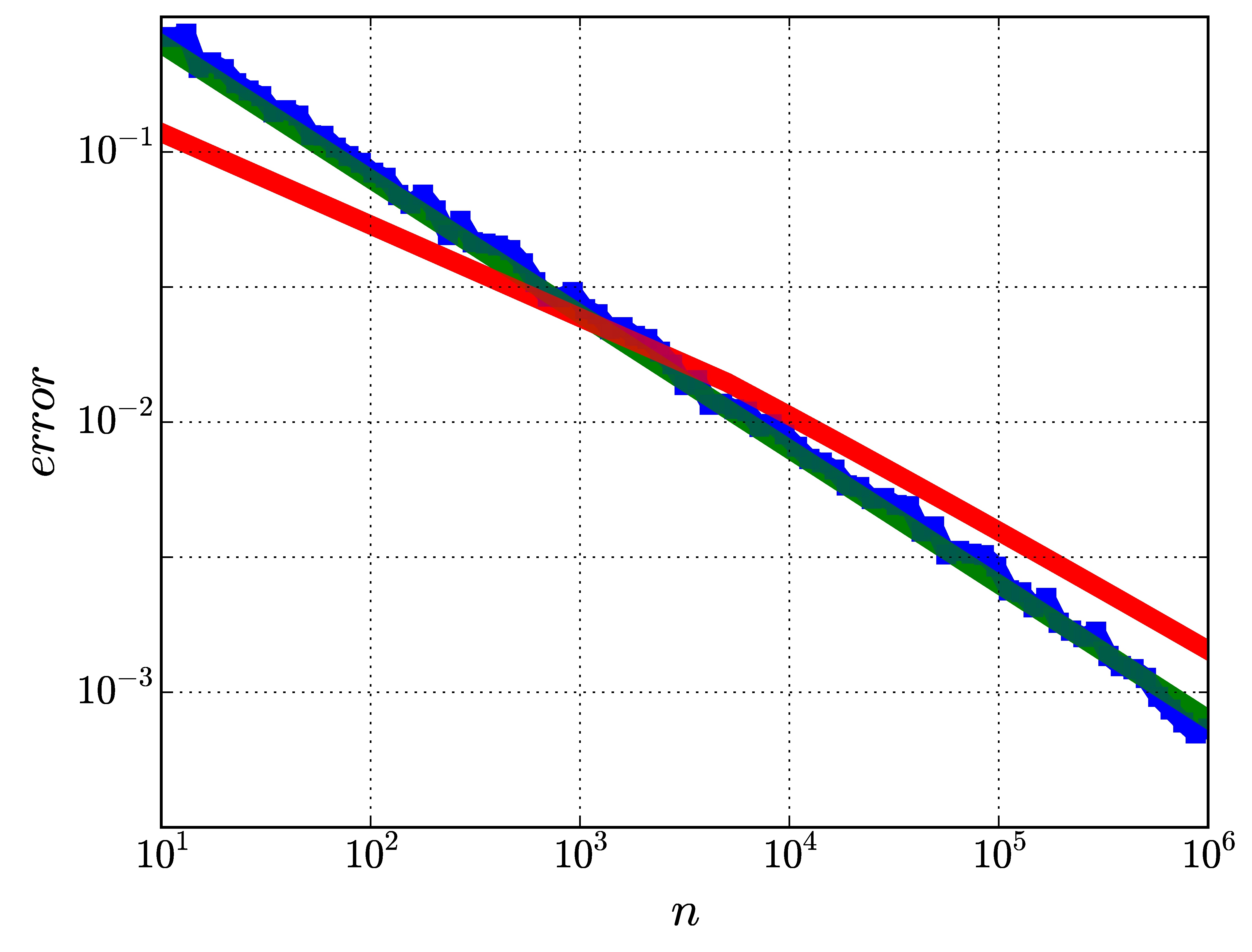
Figure 6: Log-log plots of experimental error rates (in blue) for empirical covariance fields, rates predicted by Corollary 4 (in red), and a least-squares fit of order $n^{-1/2}$ (in green).

4.3 General Kernels

We conclude the discussion of convergence of empirical CTFs with a pointwise central limit theorem (CLT) that holds for kernels in the full generality of Definition 2. One may think of it as a CLT for each entry of the matrix $\Sigma_{\alpha}(x,\sigma)$. If $e_{1},\ldots,e_{d}$ is an orthonormal basis of $\mathbb{R}^{d}$, the $(i,j)$-entry of the covariance matrix in this coordinate system is given by $\Sigma_{\alpha}(x,\sigma)(e_{i},e_{j})$, the bilinear form $\Sigma_{\alpha}(x,\sigma)$ evaluated at $(e_{i},e_{j})$. In matrix notation, this is the same as $\left\langle e_{i},\Sigma_{\alpha}(x,\sigma)e_{j}\right\rangle$. More generally, for fixed $u,v,x\in\mathbb{R}^{d}$ and $\sigma>0$, we consider

$$\Sigma_{\alpha}(x,\sigma)(u,v)=\int(y-x)\otimes(y-x)(u,v)K(x,y,\sigma)\,\alpha(dy).$$ (67)

Consider the random variable

$$z_{uv}(y)=(y-x)\otimes(y-x)\,(u,v)K(x,y,\sigma),$$ (68)

where $y$ has distribution $\alpha$. Clearly,

$$\mathbb{E}\left[z_{uv}\right]=\Sigma_{\alpha}(x,\sigma)(u,v)\,.$$ (69)

Theorem 5 (Central Limit).

If $f$ is as in Definition 2, then $z_{uv}$ has finite variance $\sigma^{2}_{uv}$. Moreover, if $z_{i}$, $i\in\mathbb{N}$, are i.i.d. random variables with the same distribution as $z_{uv}$, then

$$\sqrt{n}\left(\frac{1}{n}\sum_{i=1}^{n}z_{i}-\Sigma_{\alpha}(x,\sigma)(u,v)\right)\xrightarrow{d}\mathcal{N}(0,\sigma_{uv}^{2})\,,$$

as $n\to\infty$, where convergence is in distribution and $\mathcal{N}(0,\sigma_{uv}^{2})$ is normally distributed with mean zero and variance $\sigma_{uv}^{2}$.

Proof.

We show that $z_{uv}$ has finite second moment. From (68) and (4),

$$\begin{split}\int z^{2}_{uv}\,\alpha(dy)&\leqslant\|u\|\|v\|\int\|y-x\|^{4}K^{2}(x,y,\sigma)\,\alpha(dy)\\ &\leq\frac{\sigma^{4}\|u\|\|v\|}{C^{2}_{d}(\sigma)}\int\frac{\|y-x\|^{4}}{\sigma^{4}}f^{2}\left(\frac{\|y-x\|^{2}}{\sigma^{2}}\right)\,\alpha(dy)\\ &\leq\frac{\sigma^{4}\|u\|\|v\|}{C^{2}_{d}(\sigma)}\,C^{2}\,.\end{split}$$ (70)

The last inequality follows from condition (c) in Definition 2 that ensures that $r^{2}f^{2}(r)<C^{2}$, for any $r>0$. The theorem now follows from a direct application of the classical CLT. ∎

Remark 6.

Note that (70) implies that if $\|u\|=\|v\|=1$, then

$$\sigma^{2}_{uv}=\int z^{2}_{uv}\,\alpha(dy)-\left(\mathbb{E}\left[z_{uv}\right]\right)^{2}\leq\frac{C^{2}\sigma^{4}}{C^{2}_{d}(\sigma)}\,,$$ (71)

giving a uniform bound on the variance of $z_{uv}$ over $x\in\mathbb{R}^{d}$ and $u,v\in\mathbb{S}^{d-1}$.

5 Multiscale Fréchet Functions

The mean of a random vector $y\in\mathbb{R}^{d}$ is a simple and yet oftentimes informative, “one-element” summary of the distribution of $y$. If $y$ has finite second moment and is distributed according to the probability measure $\alpha$, then the mean may be characterized more geometrically as the unique minimizer of the Fréchet function

$$F_{\alpha}(x)=\mathbb{E}\left[\|y-x\|^{2}\right]=\int\|y-x\|^{2}\,\alpha(dy)\,,$$ (72)

which measures the spread of $y$ about $x\in\mathbb{R}^{d}$. The mean, however, is not as effective for complex distributions of practical interest such as multimodal distributions or those supported in nonlinear subspaces. In this section, we introduce a multiscale analogue of the Fréchet function that is rich in information about the shape of the distribution of $y$. At each fixed scale, the local minima of the function may be viewed as localized analogues of the mean, as illustrated in examples below. However, instead of just focusing on the local extrema, we take the view that it is more informative to investigate the behavior of the full multiscale Fréchet function, as this lets us uncover more information about the distribution of $y$.

Definition 5.

Let $f\colon[0,\infty)\to\mathbb{R}$ be as in Definition 2 with associated kernel $K\colon\mathbb{R}^{d}\times\mathbb{R}^{d}\times(0,\infty)\to\mathbb{R}$. The multiscale Fréchet function $V_{\alpha}\colon\mathbb{R}^{d}\times(0,\infty)\to\mathbb{R}$ is defined as

$$V_{\alpha}(x,\sigma):=\int\|y-x\|^{2}K(x,y,\sigma)\,\alpha(dy)\,.$$

Proposition 3.

For each $\sigma>0$, the multiscale Fréchet function satisfies

$$V_{\alpha}(x,\sigma)=\mathrm{tr}\,\Sigma_{\alpha}(x,\sigma)\,.$$

Proof.

Let $\{e_{1},\ldots,e_{d}\}\subset\mathbb{R}^{d}$ be an orthonormal basis. Then,

$$\|y-x\|^{2}=\sum_{i=1}^{d}\left\langle y-x,e_{i}\right\rangle^{2}=\sum_{i=1}^{d}(y-x)\otimes(y-x)(e_{i},e_{i})\,.$$ (73)

Hence,

$$\begin{split}V_{\alpha}(x,\sigma)&=\sum_{i=1}^{d}\int(y-x)\otimes(y-x)(e_{i},e_{i})K(x,y,\sigma)\,\alpha(dy)\\ &=\sum_{i=1}^{d}\left(\int(y-x)\otimes(y-x)K(x,y,\sigma)\,\alpha(dy)\right)(e_{i},e_{i})\\ &=\sum_{i=1}^{d}\Sigma_{\alpha}(x,\sigma)(e_{i},e_{i})=\text{tr}\,\Sigma_{\alpha}(x,\sigma)\,,\end{split}$$ (74)

as claimed. ∎

Corollary 5 (Stability).

Let $f\colon[0,\infty)\to\mathbb{R}$ be as in Definition 2 with multiscale kernel $K$. Suppose that $f$ is differentiable and there exists a constant $A>0$ such that $r^{3/2}\,|f^{\prime}(r)|\leq A$, $\forall r\geq 0$. Then, there is a constant $A_{f}>0$, that depends only on $f$, such that

$$\sup_{x\in\mathbb{R}^{d}}\left|V_{\alpha}(x,\sigma)-V_{\beta}(x,\sigma)\right|\leq\frac{\sigma dA_{f}}{C_{d}(\sigma)}\,W_{1}(\alpha,\beta),,$$

for any $\alpha,\beta\in\mathcal{P}_{1}(\mathbb{R}^{d})$ and any $\sigma>0$.

Proof.

The result follows from Proposition 3, Theorem 1 and the fact that for any $d\times d$ matrix $X$, $|\text{tr}\,X|\leq d\,\|X\|$, where $\|X\|$ is the Frobenius norm of $X$. ∎

Similarly, Corollary 1 and Proposition 3 yield the following consistency result for multiscale Fréchet functions.

Corollary 6 (Consistency).

Suppose that $\alpha\in\mathcal{P}_{1}(\mathbb{R}^{d})$. Let $y_{i}\in\mathbb{R}^{d}$, $i\in\mathbb{N}$, be i.i.d. random variables with distribution $\alpha$ and $K$ a multiscale kernel as in Theorem 1. Then, for each fixed $\sigma>0$,

$$\sup_{x\in\mathbb{R}^{d}}\left|V_{\alpha}(x,\sigma)-V_{\alpha_{n}}(x,\sigma)\right|\xrightarrow{n\uparrow\infty}0$$

almost surely.

The following result about convergence of multiscale Fréchet functions are immediate consequences of Corollary 2 and Corollary 5.

Corollary 7.

Let $f$ be as in Theorem 1 and $\sigma>0$. Suppose that $\alpha\in\mathcal{P}_{3}(\mathbb{R}^{d})$ and $y_{i}$, $i\in\mathbb{N}$, are i.i.d. random variables with distribution $\alpha$. Then, there is a constant $\beta>0$, that depends only on $d$, such that

$$\begin{split}\mathbb{E}\left[\,\sup_{x\in\mathbb{R}^{d}}\left|V_{\alpha}(x,\sigma)-V_{\alpha_{n}}(x,\sigma)\right|\right]&\leq\\ \frac{\sigma dA_{f}\beta}{C_{d}(\sigma)}m_{3}(\alpha)&\cdot\begin{cases}n^{-\frac{2}{3}}+n^{-\frac{1}{2}}&\text{if $d=1$;}\\ n^{-{\frac{2}{3}}}+n^{-\frac{1}{2}}\log(1+n)&\text{if $d=2$;}\\ n^{-\frac{2}{3}}+n^{-\frac{1}{d}}&\text{if $d\geq 3$.}\end{cases}\end{split}$$

Remark 7.

Analogous stability and consistency results for the truncation kernel follow from Theorem 3, Corollary 3 and Corollary 4.

For more general kernels, the following pointwise central limit theorem holds. For fixed $x\in\mathbb{R}^{d}$ and $\sigma>0$, let

$$t(y)=\|y-x\|^{2}K(x,y,\sigma),$$ (75)

whose expected value is $\mathbb{E}\left[t\right]=V_{\alpha}(x,\sigma)$. As in Theorem 5, the variance of $t$ is finite and denoted $\sigma^{2}_{t}$.

Theorem 6 (Central Limit).

Let $f$ be as in Definition 2. If $t_{i}\in\mathbb{R}$, $i\in\mathbb{N}$, are i.i.d. random variables with the same distribution as $t$, then

$$\sqrt{n}\left(\frac{1}{n}\sum_{i=1}^{n}t_{i}-V_{\alpha}(x,\sigma)\right)\xrightarrow{d}\mathcal{N}(0,\sigma_{t}^{2})\,,$$

as $n\to\infty$, where convergence is in distribution and $\mathcal{N}(0,\sigma_{V}^{2})$ is normally distributed with mean zero and variance $\sigma_{t}^{2}$.

Multiscale Fréchet functions not only give stable representations of probability measures, but any probability measure $\alpha$ may be fully recovered from its multiscale Fréchet function associated with the Gaussian kernel, as the following result shows.

Proposition 4.

Let $\sigma>0$ be fixed. Any probability measure $\alpha$ is completely determined by the Fréchet function $V_{\alpha}(\cdot,\sigma)$ associated with the Gaussian kernel at scale $\sigma$.

Proof.

Let $h_{\sigma}\colon\mathbb{R}^{d}\to\mathbb{R}$ be given by

$$h_{\sigma}(x)=\frac{\|x\|^{2}}{(2\pi\sigma^{2})^{d/2}}\exp{\left(-\frac{\|x\|^{2}}{2\sigma^{2}}\right)}\,.$$ (76)

Then, for the Gaussian kernel, we may express the multiscale Fréchet function as the convolution $V_{\alpha}(x,\sigma)=(h_{\sigma}\ast\alpha)(x)$. Under Fourier transform, for each fixed $\sigma>0$, we obtain

$$\widehat{V}_{\alpha}(\xi,\sigma)=\widehat{h}_{\sigma}(\xi)\,\phi_{\alpha}(-2\pi\xi)\,,$$ (77)

where $\phi_{\alpha}$ is the characteristic function of $\alpha$ defined as $\phi_{\alpha}(\xi)=\int e^{i\left\langle x,\xi\right\rangle}\,\alpha(dx)$. Therefore,

$$\phi_{\alpha}(\xi)=\widehat{V}_{\alpha}(-\xi/2\pi,\sigma)/\,\widehat{h}_{\sigma}(-\xi/2\pi)$$ (78)

provided that $\widehat{h}_{\sigma}(-\xi/2\pi)\neq 0$. A calculation shows that

$$\widehat{h}_{\sigma}(-\xi/2\pi)=\sigma^{2}\left(d-\frac{\sigma^{2}\|\xi\|^{2}}{\pi}\right)\exp{\left(-\frac{\sigma^{2}\|\xi\|^{2}}{2\pi}\right)}\,,$$ (79)

which only vanishes at points $\xi$ on the sphere of radius $\rho_{\sigma}=\sqrt{\pi d}/\sigma$ about the origin. Thus, (78) implies that we can recover $\phi_{\alpha}(\xi)$ from $\widehat{V}_{\alpha}(\cdot,\sigma)$, if $\|\xi\|\neq\sqrt{\pi d}/\sigma$. By continuity, we can recover $\phi_{\alpha}(\xi)$, for any $\xi$. The claim now follows from the fact that the characteristic function $\phi_{\alpha}$ determines $\alpha$ [35]. ∎

The following examples illustrate how information about the shape of data can be extracted from multiscale Fréchet functions.

Example 7.

We consider $n=400$ data points distributed into two clusters of 200 points, each sampled from a Gaussian of variance $0.36$ centered at different points. The data points are plotted in blue in Fig. 7(a), which also shows the empirical Fréchet function $V_{n}$ at scale $\sigma=3$. The local minima of $V_{n}$ captures what is perceived as the “centers” of the two clusters at that scale. However, more information about the data distribution can be uncovered from $V_{n}$. For example, the local minima may be viewed as attractors of the (negative) gradient field $-\nabla V_{n}$, indicated by the arrows in the figure. The stable manifold of each attractor, which comprises points that move toward the attractors under the associated flow may be viewed as clusters inferred from the data at that scale. These clusters are delimited by the repellers of the system, which correspond to the local maxima of $V_{n}$. Fig. 7(b) shows how $V_{n}$ varies across scales, highlighting the bifurcation of the attractors (in red) and repellers (in green) as $\sigma$ changes.

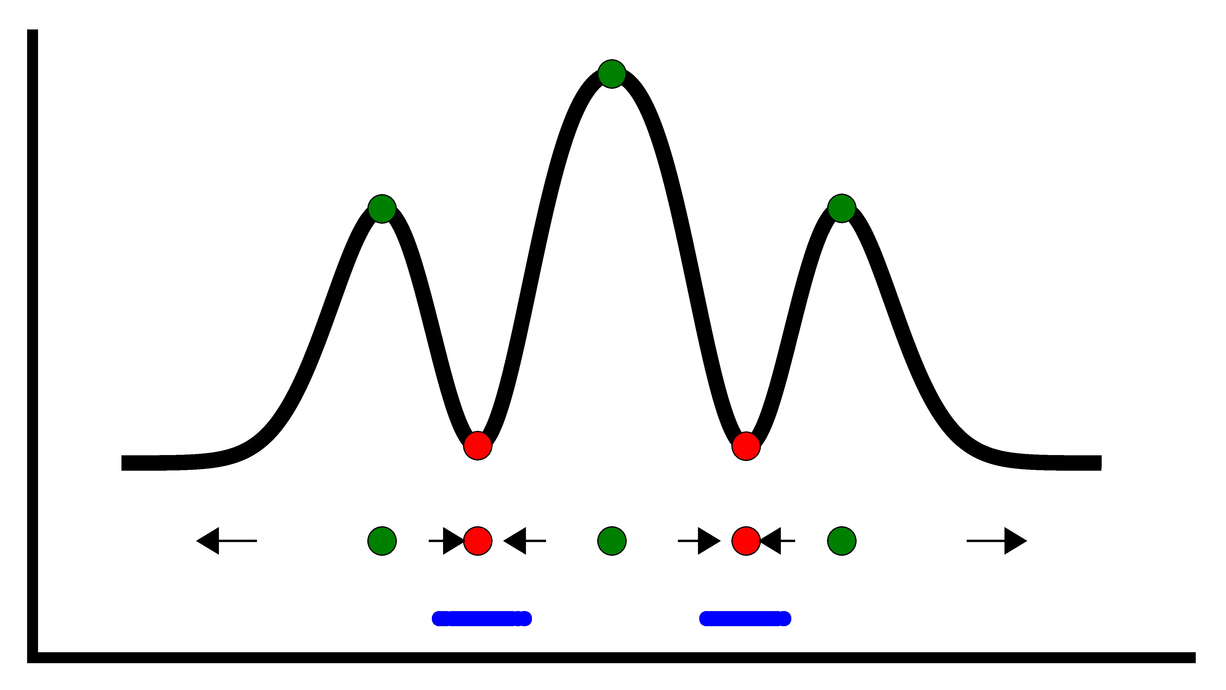
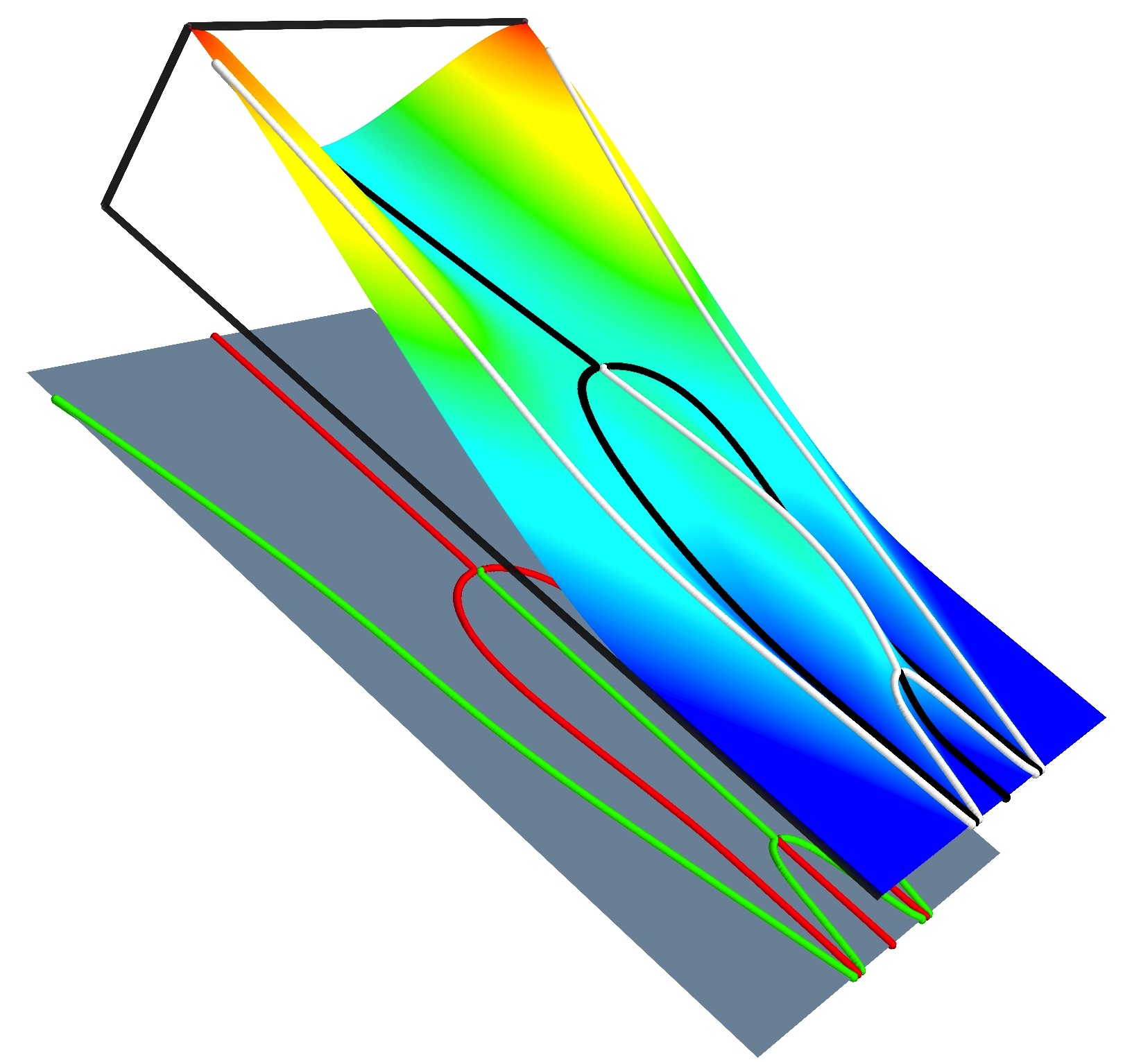
(a)	(b)

Figure 7: (a) Fréchet function for data on the line (highlighted in blue) computed with the Gaussian kernel at scale $\sigma=3$; (b) Fréchet function across scales.

In data analysis, such bifurcation diagrams may find several applications. For example, if the data represent the distribution of some phenotypic trait for two species that have evolved from a single group, the multiscale Fréchet function and the associated bifurcation diagram let us create an evolutionary model for the trait from the observed data.

Example 8.

Here we consider the dataset in $\mathbb{R}^{2}$ shown in panel (a) of Fig. 8. Panels (b)–(h) show the Fréchet function for the Gaussian kernel calculated at increasing scales. The gradient field $-\nabla V_{n}$ at scale $\sigma=2.25$ is depicted in panel (a) of Fig. 9 along with the two attractors $p_{1}$ and $p_{2}$, and their stable manifolds that were estimated numerically.

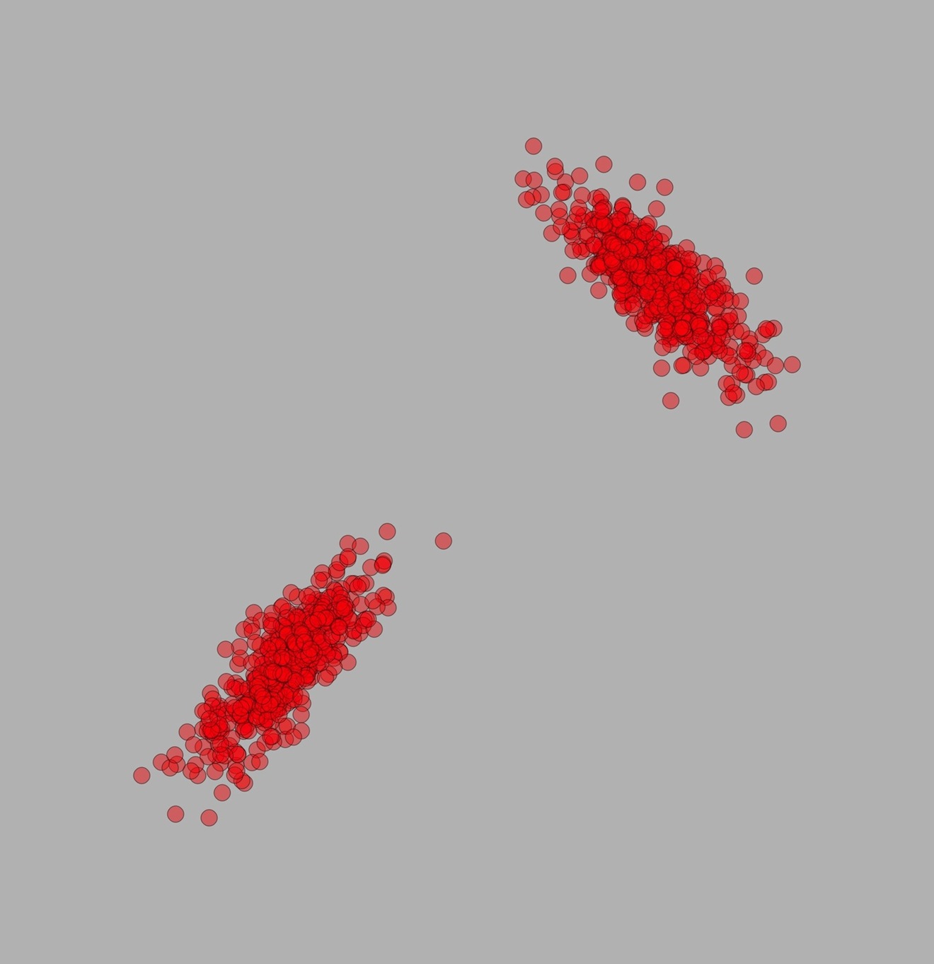
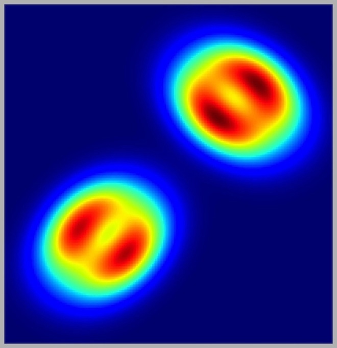
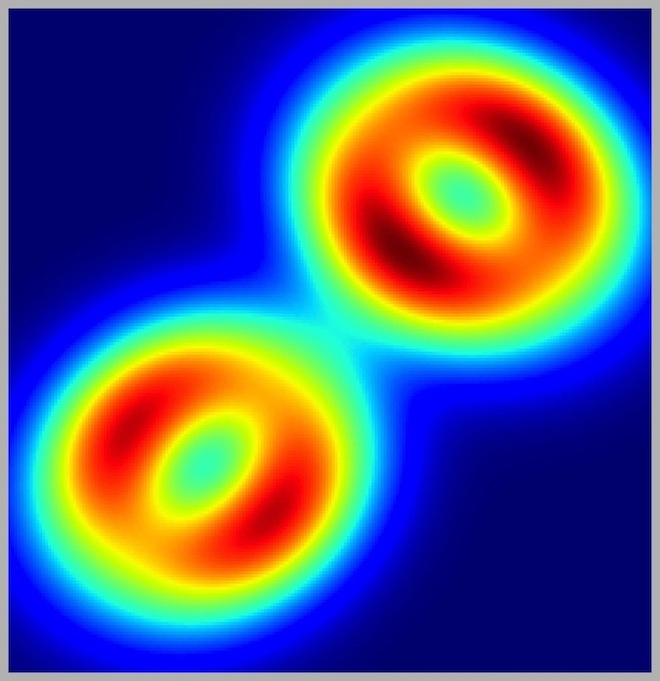
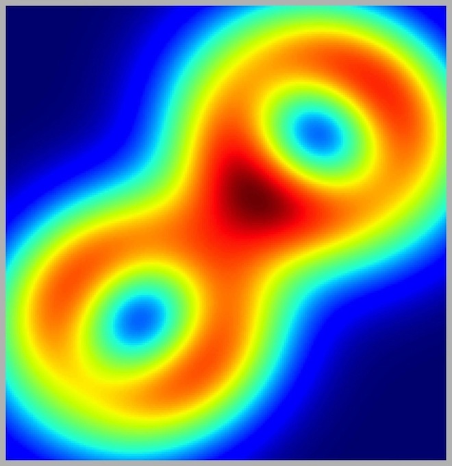
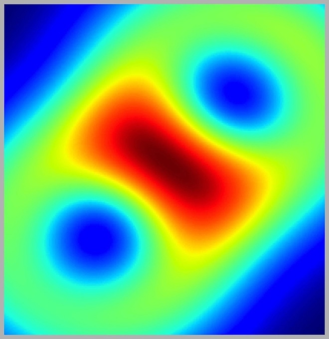
data	$\sigma=$1.0	$\sigma=1.5$	$\sigma=2.0$	$\sigma=3.0$
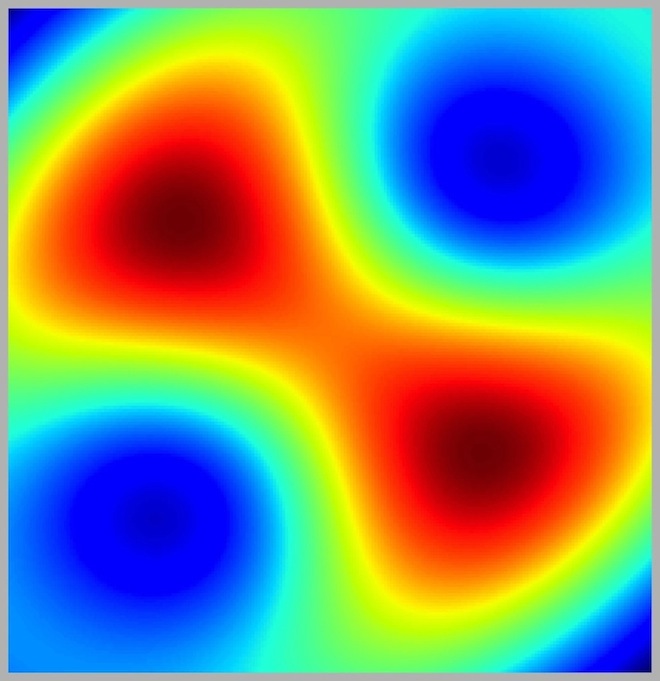
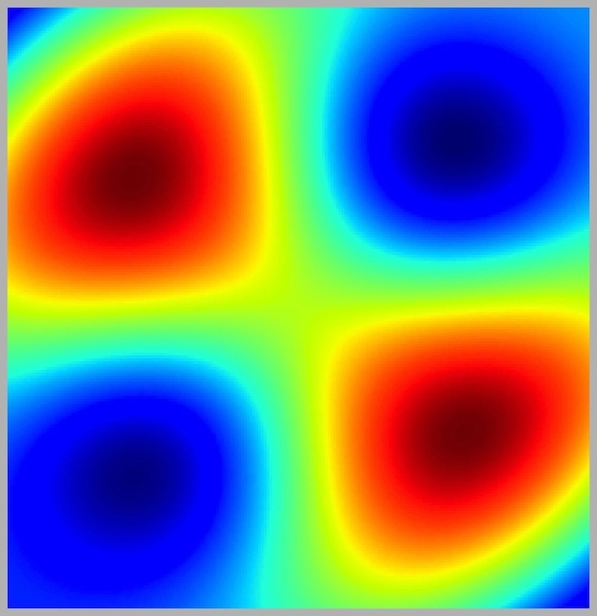
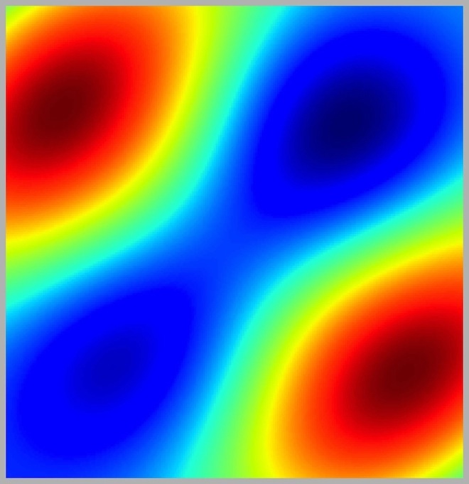
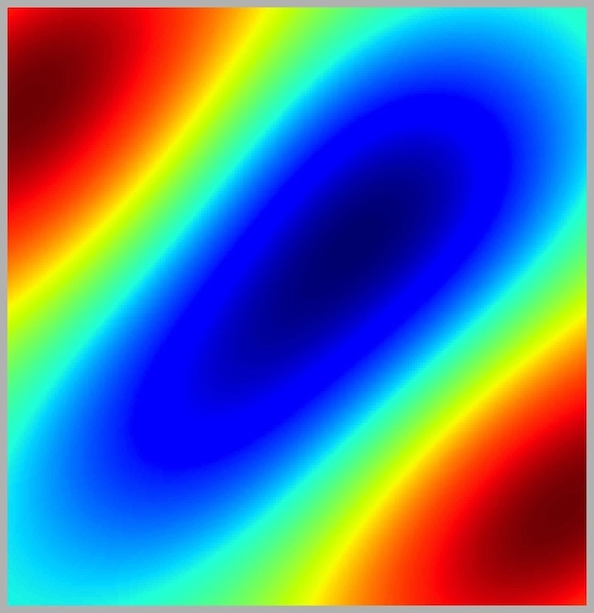
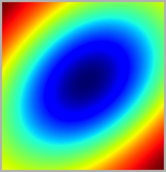
$\sigma=4.5$	$\sigma=5.0$	$\sigma=6.0$	$\sigma=7.0$	$\sigma=9.0$

Figure 8: Heat maps of the multiscale Fréchet function for 2D data at increasing scales computed with the Gaussian kernel.

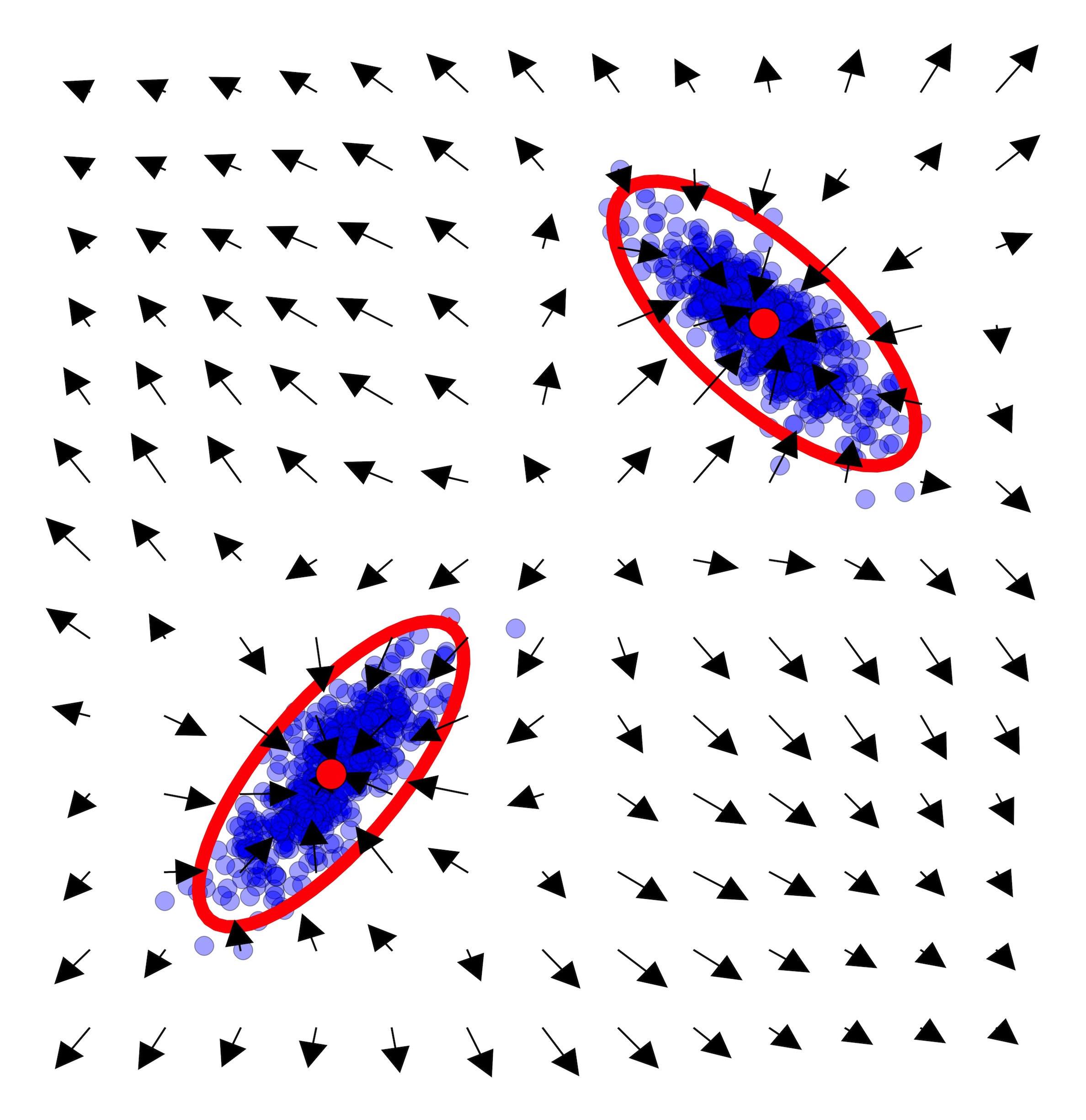
(a)	(b)

Figure 9: (a) 2D data, attractors and their stable manifolds at a fixed scale ($\sigma=2.25$); (b) gradient vector field and covariance tensors at the attractors.

The stable manifolds may be viewed as estimations at scale $\sigma=2.25$ of clusters of the underlying probability measure $\alpha$ from which the data was sampled. Panel (b) shows the gradient field and the covariance tensors at the attractors depicted as ellipses with principal radii proportional to the square root of the eigenvalues of the covariance matrix. This may be viewed as a localized analogue of principal component analysis (PCA) that is able to uncover geometry that is not detectable with standard PCA. Analysis of the spectra of $\Sigma_{n}(p_{i},\sigma)$, $i=1,2$, suggests that the data is organized around two one-dimensional clusters, whereas standard PCA is not sensitive to the local dimensionality because of the orientation of the clusters.

These examples are intended as proof-of-concept illustrations. Topological and other methods will be explored in forthcoming work for extraction of structural information from $V_{n}$.

6 Hierarchical Manifold Clustering

Clustering is a central theme in pattern analysis with a rich history; cf. [36]. One of the most studied forms of the problem is that of partitioning a dataset into various subsets if there is some form of spatial separation of the data into subgroups. Motivated by problems in such areas as computer vision and video analysis, cf. [37], there has been a growing interest in clustering data that are organized as a finite union of possibly intersecting subspaces that have some special geometric structure [38, 16, 18, 26]. As illustrated in Fig. 1, the data may consist of noisy samples from an arrangement of (affine) linear subspaces of a Euclidean space such as a collection of lines in a plane, or an arrangement of lines and planes in $\mathbb{R}^{3}$. More generally, the clusters may comprise a finite collection of possibly non-linear, smooth submanifolds of a Euclidean space that intersect transversely. Here we propose an approach to manifold clustering based on CTFs. The basic idea is to use covariance fields to incorporate directional information at each data point. Formally, this is achieved via a section of the tensor bundle $\mathbb{R}^{d}\times(\mathbb{R}^{d}\otimes\mathbb{R}^{d})$ over $\mathbb{R}^{d}$, as follows. Given a probability measure $\alpha$ and a multiscale kernel, let $\Sigma_{\alpha}(x,\sigma)$ be the associated CTF. For each $\sigma>0$, consider the section $\iota_{\alpha;\sigma}\colon\mathbb{R}^{d}\to\mathbb{R}^{d}\times(\mathbb{R}^{d}\otimes\mathbb{R}^{d})$ given by $x\mapsto\left(x,\Sigma_{\alpha}(x,\sigma)\right)$. On the total space of the tensor bundle, define the metric

$$\|(x,\Sigma)-(x^{\prime},\Sigma^{\prime})\|_{\gamma}=\left(\|\Sigma-\Sigma^{\prime}\|^{2}+\gamma^{2}\|x-x^{\prime}\|^{2}\right)^{1/2}\,,$$ (80)

where $x,x^{\prime}\in\mathbb{R}^{d}$, $\Sigma,\Sigma^{\prime}\in\mathbb{R}^{d}\otimes\mathbb{R}^{d}$, and $\gamma\geq 0$ is a parameter that balances the contributions of the spatial and tensor components. Note that $\|\cdot\|_{0}$ only defines a pseudo-metric since $\|\cdot\|_{0}$ disregards “horizontal” distances.

For any subset $X\subseteq\mathbb{R}^{d}$, we denote by $\mathbb{X}_{\alpha;\gamma,\sigma}$ the metric space $(X,d_{\alpha;\gamma,\sigma})$, where

$$d_{\alpha;\gamma,\sigma}(x,x^{\prime})=\left\|\iota_{\alpha;\sigma}(x)-\iota_{\alpha;\sigma}(x^{\prime})\right\|_{\gamma}\,.$$ (81)

For a dataset $A=\{a_{1},\ldots,a_{n}\}\subset\mathbb{R}^{d}$, the proposed clustering method is based on the single-linkage method [39] applied to the finite metric space $\mathbb{A}_{\alpha_{n};\gamma,\sigma}$ associated with the empirical measure $\alpha_{n}=n^{-1}\sum_{i=1}^{n}\delta_{a_{i}}$. Equivalently, clustering is based on the $n\times n$ affinity matrix $D$ whose $(i,j)$-entry is

$$d_{ij}=d_{\alpha_{n};\gamma,\sigma}(a_{i},a_{j})\,.$$ (82)

Recall that single linkage on a finite metric space $\mathbb{A}=(A,d_{A})$ starts from $n$ clusters, each a singleton $\{a_{i}\}$, $1\leqslant i\leqslant n$, sequentially merging the closest clusters until all data points coalesce into a single cluster. Closeness of two clusters, say $A_{1},A_{2}\subset A$, is measured by the inter-cluster distance

$$d_{sl}(A_{1},A_{2})=\min_{a\in A_{1},a^{\prime}\in A_{2}}d_{A}(a,a^{\prime})\,,$$ (83)

We choose single linkage because it yields stable dendrograms, as expounded below, under assumptions on the probability measure from which the data is sampled that are not very restrictive. Combined with our stability and consistency results for covariance fields, this guarantees that the manifold clustering method is stable at all stages.

6.1 Dendrogram Stability

We denote a metric space by $\mathbb{X}=(X,d_{X})$. An ultrametric space is a pair $(X,u_{X})$, where $u_{X}\colon X\times X\to\mathbb{R}^{+}$ is a metric on $X$ that satisfies the strong triangle inequality

$$u_{X}(x,x^{\prime})\leq\max\left\{u_{X}(x,x^{\prime\prime}),u_{X}(x^{\prime\prime},x^{\prime})\right\}\,,$$ (84)

for all $x,x^{\prime},x^{\prime\prime}\in X$. Any such function $u_{X}$ is called an ultrametric on $X$.

As proved in [32], dendrograms over a finite set $X$ are in structure-preserving, bijective correspondence with ultrametrics on $X$. In this formulation, a hierarchical clustering method can be regarded as a map $\mathcal{H}:\mathcal{M}\rightarrow\mathcal{U}$ from finite metric spaces into finite ultrametric spaces. Henceforward, $\mathcal{H}$ will denote the map given by single linkage hierarchical clustering. It is known [32] that if $\mathbb{X}=(X,d_{X})\in\mathcal{M}$, then $\mathcal{H}(\mathbb{X})=(X,u_{X})$ is given by

$$u_{X}(x,x^{\prime})=\min_{x=x_{0},\ldots,x_{r}=x^{\prime}}\max_{i}d_{X}(x_{i},x_{i+1})\,.$$ (85)

The minimum above is taken over all finite ordered sequences $x_{0},x_{1},\ldots,x_{r}$ of points in $X$ such that $x_{0}=x$ and $x_{r}=x^{\prime}$. If $x,x^{\prime}\in X$, then $u_{X}(x,x^{\prime})$ may be interpreted as the dendrogram level at which the clusters containing $x$ and $x^{\prime}$ first merge. This is known as the cophenetic distance between $x$ and $x^{\prime}$.

The main goal of this section is to formulate and prove stability of the map $\mathcal{M}\ni\mathbb{X}\mapsto\mathcal{H}(\mathbb{X})\in\mathcal{U}$. The question of stability of single linkage clustering can be approached using ideas related to the Gromov-Hausdorff distance [40], as follows. A correspondence $R$ between two sets $X$ and $Y$ is a subset of $X\times Y$ such that $\pi_{1}(R)=X$ and $\pi_{2}(R)=Y$, where $\pi_{1}$ and $\pi_{2}$ denote projections onto the first and second factors. Given $X$ and $Y$, we denote by $\mathcal{R}(X,Y)$ the set of all correspondences between $X$ and $Y$.

Definition 6.

Let $\mathbb{X}$ and $\mathbb{Y}$ be compact metric spaces.

• The distortion of a correspondence $R$ between $\mathbb{X}$ and $\mathbb{Y}$ is defined by

  $$\text{dis}\,(R;\mathbb{X},\mathbb{Y}):=\max_{(x,y),(x^{\prime},y^{\prime})\in R}\left|d_{X}(x,x)-d_{Y}(y,y^{\prime})\right|.$$

• The Gromov-Hausdorff distance between $\mathbb{X}$ and $\mathbb{Y}$ is given by

  $$d_{GH}(\mathbb{X},\mathbb{Y}):=\frac{1}{2}\inf_{R}\text{dis}\,(R;\mathbb{X},\mathbb{Y}),$$

  where the infimum is taken over all correspondences between $\mathbb{X}$ and $\mathbb{Y}$.

The following stability result is a generalization of [32, Proposition 26].

Proposition 5.

For any $\mathbb{X},\mathbb{Y}\in\mathcal{M}$ and any correspondence $R\in\mathcal{R}(X,Y)$,

$$\mathrm{dis}(R;\mathcal{H}(\mathbb{X}),\mathcal{H}(\mathbb{Y}))\leq\mathrm{dis}(R;\mathbb{X},\mathbb{Y})\,.$$

As a consequence, $d_{GH}(\mathcal{H}(\mathbb{X}),\mathcal{H}(\mathbb{Y}))\leq d_{GH}(\mathbb{X},\mathbb{Y})$.

Remark 8.

The claim of the proposition may be written, equivalently, as follows. If $u_{X}$ and $u_{Y}$ denote the ultrametrics produced by single linkage hierarchical clustering on $\mathbb{X}$ and $\mathbb{Y}$, then

$$|u_{X}(x,x^{\prime})-u_{Y}(y,y^{\prime})|\leq\max_{(x,y),(x^{\prime},y^{\prime})\in R}|d_{X}(x,x^{\prime})-d_{Y}(y,y^{\prime})|\,,$$ (86)

for any correspondence $R$ between $X$ and $Y$ and all $(x,y),(x^{\prime},y^{\prime})\in R$.

Proof of Proposition 5.

We prove (86). Given a correspondence $R\in\mathcal{R}(X,Y)$ and $(x,y),(x^{\prime},y^{\prime})\in R$, let $x=x_{0},x_{1},\ldots,x_{n}=x^{\prime}$ in $X$ be such that $\max_{i}d_{X}(x_{i},x_{i+1})=u_{X}(x,x^{\prime})$. Let $y_{0}=y$, $y_{n}=y^{\prime}$ and choose $y_{1},\ldots,y_{n-1}\in Y$ such that $(x_{i},y_{i})\in R$ for all $i=1,\ldots,n-1$. This is possible since any correspondence $R$ satisfies $\pi_{1}(R)=X$. Notice that

$$\begin{split}u_{Y}(y,y^{\prime})&\leq\max_{i}d_{Y}(y_{i},y_{i+1})\\ &\leq\max_{i}\left(d_{X}(x_{i},x_{i+1})+|d_{X}(x_{i},x_{i+1})-d_{Y}(y_{i},y_{i+1})|\right)\\ &\leq\max_{i}d_{X}(x_{i},x_{i+1})+\max_{(x,y),(x^{\prime},y^{\prime})\in R}|d_{X}(x,x^{\prime})-d_{Y}(y,y^{\prime})|\\ &=u_{X}(x,x^{\prime})+\max_{(x,y),(x^{\prime},y^{\prime})\in R}|d_{X}(x,x^{\prime})-d_{Y}(y,y^{\prime})|.\end{split}$$ (87)

The claim follows since (87) also holds if we reverse the roles of $X$ and $Y$. ∎

Lemma 2.

Let $\alpha,\beta\in\mathcal{P}_{\infty}(\mathbb{R}^{d})$ and $\sigma>0$. If a kernel satisfies the conditions of Lemma 1, then

$$\sup_{(a,b)\in R_{\mu}}\left\|\Sigma_{\alpha}(a,\sigma)-\Sigma_{\beta}(b,\sigma)\right\|\leq\frac{2A_{f}\sigma}{C_{d}(\sigma)}\,\sup_{(a,b)\in R_{\mu}}\|a-b\|\,,$$

for any coupling $\mu\in\Gamma(\alpha,\beta)$, where $R_{\mu}:=\text{supp}\,[\mu]$ and $A_{f}>0$ is as in Lemma 1.

Proof.

Set $\zeta=\sup_{(a,b)\in\text{supp}\,[\mu]}\|a-b\|$. Let $\mu\in\Gamma(\alpha,\beta)$ and $(y,y^{\prime}),(a,b)\in\text{supp}\,[\mu]$. In the notation of Lemma 1, setting $z_{1}=y-a$ and $z_{2}=y^{\prime}-b$, we have

$$\|Q_{\sigma}(y-a)-Q_{\sigma}(y^{\prime}-b)\|\leq\frac{A_{f}\sigma}{C_{d}(\sigma)}\left(\|y-y^{\prime}\|+\|a-b\|\right)\leq\frac{2A_{f}\sigma}{C_{d}(\sigma)}\zeta\,,$$ (88)

where in the last inequality we used $\|y-y^{\prime}\|\leq\zeta$ and $\|a-b\|\leq\zeta$. Since

$$\left\|\Sigma_{\alpha}(a,\sigma)-\Sigma_{\beta}(b,\sigma)\right\|\leq\iint\|Q_{\sigma}(y-a)-Q_{\sigma}(y^{\prime}-b)\|\,\mu(dy\times dy^{\prime})\,,$$ (89)

the lemma follows. ∎

Lemma 3 (Lemma 2.2 of [41]).

Let $\alpha,\beta\in\mathcal{P}_{\infty}(\mathbb{R}^{d})$. Then, for any coupling $\mu\in\Gamma(\alpha,\beta)$, $R_{\mu}=\text{supp}\,[\mu]$ gives a correspondence between $A=\text{supp}\,[\alpha]$ and $B=\text{supp}\,[\beta]$.

Theorem 7.

Let $\alpha,\beta\in\mathcal{P}_{\infty}(\mathbb{R}^{d})$, $A=\text{supp}\,[\alpha]$, $B=\text{supp}\,[\beta]$, $\sigma>0$ and $\gamma\geq 0$. Then, for any kernel satisfying the conditions of Lemma 1,

$$d_{GH}\left((A,d_{\alpha;\sigma,\gamma}),(B,d_{\beta;\sigma,\gamma})\right)\leq\left(\frac{2A_{f}\sigma}{C_{d}(\sigma)}+\gamma\right)W_{\infty}(\alpha,\beta)\,,$$

with $A_{f}>0$ as in Lemma 1.

Proof.

Let $\mu\in\Gamma(\alpha,\beta)$ be a coupling that realizes $W_{\infty}(\alpha,\beta)$. By Lemma 3, $R_{\mu}=\text{supp}\,[\mu]$ is a correspondence between $A$ and $B$. Thus,

$$\begin{split}d_{GH}\big{(}\mathbb{A}_{\alpha;\sigma,\gamma},\,&\mathbb{B}_{\beta;\sigma,\gamma}\big{)}\leq\frac{1}{2}\,\text{dis}(R_{\mu};A,B)\\ &=\frac{1}{2}\sup_{(a,b),(a^{\prime},b^{\prime})\in R_{\mu}}\left|d_{\alpha;\sigma,\gamma}(a,a^{\prime})-d_{\beta;\sigma,\gamma}(b,b^{\prime})\right|\\ &\leq\frac{1}{2}\sup_{(a,b),(a^{\prime},b^{\prime})\in R_{\mu}}\Big{(}\left\|\Sigma_{\alpha}(a,\sigma)-\Sigma_{\beta}(b,\sigma)\right\|+\\ &+\big{\|}\Sigma_{\alpha}(a^{\prime},\sigma)-\Sigma_{\beta}(b^{\prime},\sigma)\big{\|}+\gamma\|a-b\|+\gamma\|a^{\prime}-b^{\prime}\|\Big{)}\\ &\leq\sup_{(a,b)\in R_{\mu}}\left\|\Sigma_{\alpha}(a,\sigma)-\Sigma_{\beta}(b,\sigma)\right\|+\gamma\sup_{(a,b)\in R_{\mu}}\|a-b\|\\ &\leq\left(\frac{2A_{f}\sigma}{C_{d}(\sigma)}+\gamma\right)\sup_{(a,b)\in R_{\mu}}\|a-b\|,\end{split}$$ (90)

where the last step follows from Lemma 2. The conclusion follows since $W_{\infty}(\alpha,\beta)=\sup_{(a,b)\in R_{\mu}}\|a-b\|.$ ∎

Combining Proposition 5 and Theorem 7, we obtain:

Corollary 8 (Stability of Hierarchical Manifold Clustering).

Let $\alpha,\beta\in\mathcal{P}_{\infty}(\mathbb{R}^{d})$ be probability measures with finite support, $A=\text{supp}\,[\alpha]$, $B=\text{supp}\,[\beta]$, $\sigma>0$ and $\gamma\geq 0$. Then,

$$d_{GH}\left(\mathcal{H}(\mathbb{A}_{\alpha;\gamma,\sigma}),\mathcal{H}(\mathbb{B}_{\alpha;\gamma,\sigma})\right)\leq\left(\frac{2A_{f}\sigma}{C_{d}(\sigma)}+\gamma\right)W_{\infty}(\alpha,\beta).$$

6.2 Comments About Consistency of Hierarchical Manifold Clustering

A question that our paper leaves open is whether, under a reasonable generative model for the sampling from a collection of intersecting manifolds one may be able to prove that the empirical dendrogram converges in probability to a dendrogram that represents the spatial organization of the underlying manifolds. In the simpler context of clustering $n$ i.i.d. samples $\{x_{1},\ldots,x_{n}\}$ from a compact metric space $(X,d_{X})$ endowed with a Borel probability measure $\alpha_{X}$, it has been established in [32] that single linkage hierarchical clustering converges to a dendrogram whose hierarchical structure depends on the support of $\alpha_{X}$ in a precise way.

In the case of flat clustering, i.e. when the goal is to obtain a single partition of the dataset, consistency results for some multi-manifold clustering methods based on local PCA are given in [16, 17, 18].

6.3 Examples and Applications

Let $X=\{x_{1},\ldots,x_{n}\}$ be a dataset in $\mathbb{R}^{d}$. For $\gamma,\sigma>0$, we apply the single linkage method to the metric space $\mathbb{X}_{\alpha_{n};\gamma,\sigma}=(X,d_{\alpha_{n};\gamma,\sigma})$, where $\alpha_{n}$ is the empirical measure associated with $X$ and $d_{\alpha_{n};\gamma,\sigma}$ is the distance defined in (81). The ultrametric associated with $\mathcal{H}(\mathbb{X}_{\alpha_{n};\gamma,\sigma})$ is abbreviated $u_{\alpha_{n};\gamma,\sigma}$.

In this setting, analyzing informative dendrogram cutoff levels often is an important task, which can be approached in different ways, depending on the nature of the problem. For example, a cutoff level $h$ may be based on a pre-assigned number of clusters, be learned from training data, or be more exploratory. We give examples that illustrate all three viewpoints.

Example 9 (Lines and planes).

In this experiment we consider the unlabeled point cloud in Fig. 1(a) that represents an arrangement of two parallel planes and two lines that intersect the planes transversely. Each plane contains $225$ points on a uniform grid and each line contains $30$ equally spaced points. Cutting the dendrogram at four clusters, our method finds the four affine linear subspaces accurately with the Gaussian kernel at $\sigma=0.6$. In this case, it is important to choose $\gamma\neq 0$ since the spatial component of (82) is needed to discriminate the parallel planes. In Fig. 1(a), the points are colored according to cluster membership. In this case, the covariance tensors at data points on the planes that are away ’from the cluster intersections have two dominating eigenvalues, whereas for points on the lines they have only one such eigenvalue. Thus, an analysis of the spectrum of the covariance tensors at data points let us infer the dimension of each cluster.

Example 10 (A Line Arrangement).

In this example, the point-cloud data represents three intersecting lines in $\mathbb{R}^{2}$, as shown in Fig. 10(a). Each line segment is sampled at $200$ equally spaced points. Since the slopes of the lines are different, we expect the covariance matrices to be able to cluster the points without the aid of additional spatial information. Thus, we set $\gamma=0$ in (82) and $\sigma=0.4$. The number of clusters was set to six to test the ability of the algorithm to detect not only the lines, but also the three intersections. Fig. 10(b) shows the single-linkage dendrogram, highlighting each of the six clusters. The data points are colored according to cluster membership.

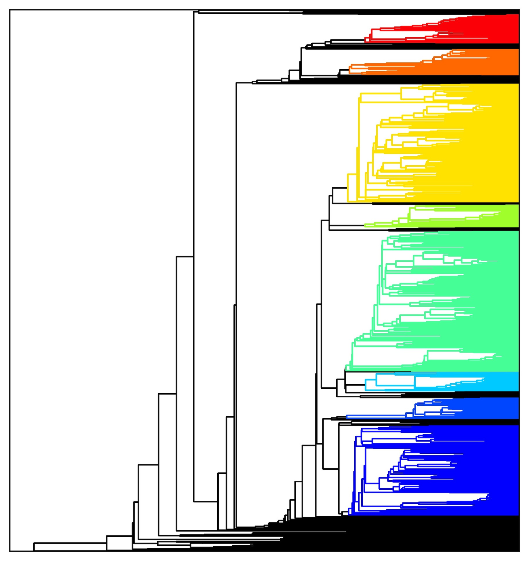
(a)	(b)	(c)	(d)

Figure 10: (a) an arrangement of three lines and (b) clustering dendrogram; (c) noisy lines with outliers and (d) clustering dendrogram.

As expected, well delineated clusters are detected away from the intersection points because the covariance matrices are highly anisotropic with principal axes that align well with the corresponding line segments. Although the covariance matrices are not as anisotropic near the intersection points, there are enough differences in their behavior near the three intersection loci for the algorithm to be able to place them into different clusters.

The next two examples are of a more exploratory nature in that dendrogram cutoff was chosen through experimentation with the data.

Example 11 (Noisy Lines with Outliers).

This is a noisy version of Example 10, as shown in Fig. 10(c). As before, each line is represented by 200 points, but we have added Gaussian noise of width $0.015$ to the data, as well as 180 outliers sampled from the uniform distribution on a rectangle containing the lines. Because of the nature of the data, the number of clusters was set to $m=80$ so that the three main clusters did not get merged because of the outliers. The figure also shows a line fitted to each of the three largest clusters using principal component analysis. The method was able to sharply recover the three lines, even in the presence of noise and outliers. The majority of the 80 clusters are singletons of outliers and these are colored black in the figure. We remark that the choice of $\sigma=0.51$ is crucial when dealing with data contaminated by noise. In this case, it was also important to set $\gamma\neq 0$ to better cope with noise.

Example 12 (Floor cracks).

We apply the clustering method to segmentation of two images of concrete floor cracks. Panel (a) of Fig. 11 shows the original images, whereas panel (b) shows binary images obtained from an edge detection algorithm. We cluster the foreground pixels of the binary images. As in Example 11, it is important to allow a fairly large number of clusters so that the clusters that detect the main cracks do not get merged because of the noisy pixels. Panels (c) and (d) show the outputs (not to scale) of the clustering algorithm.

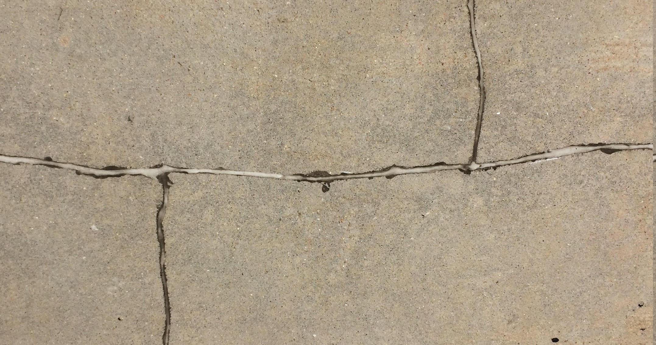
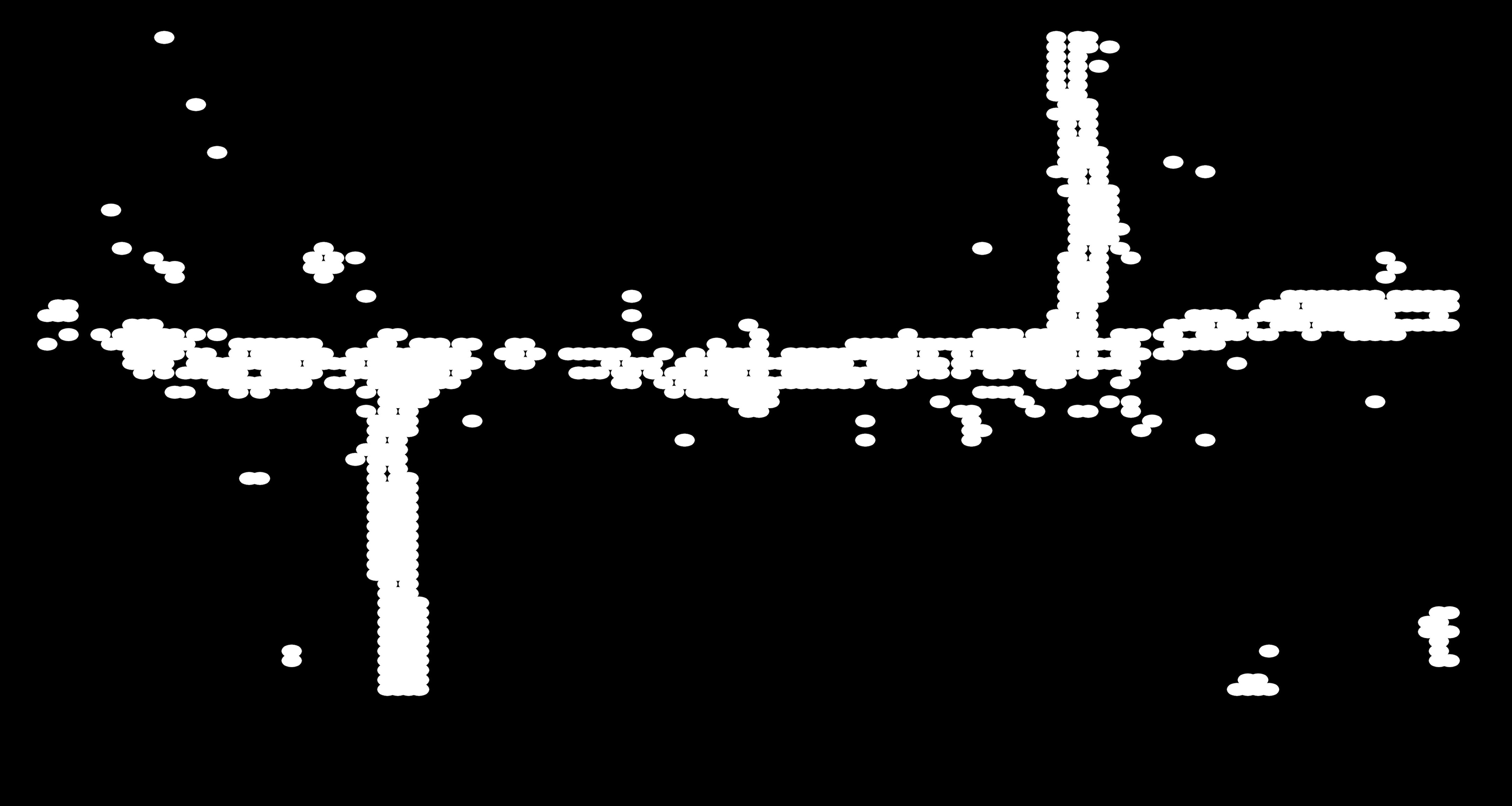
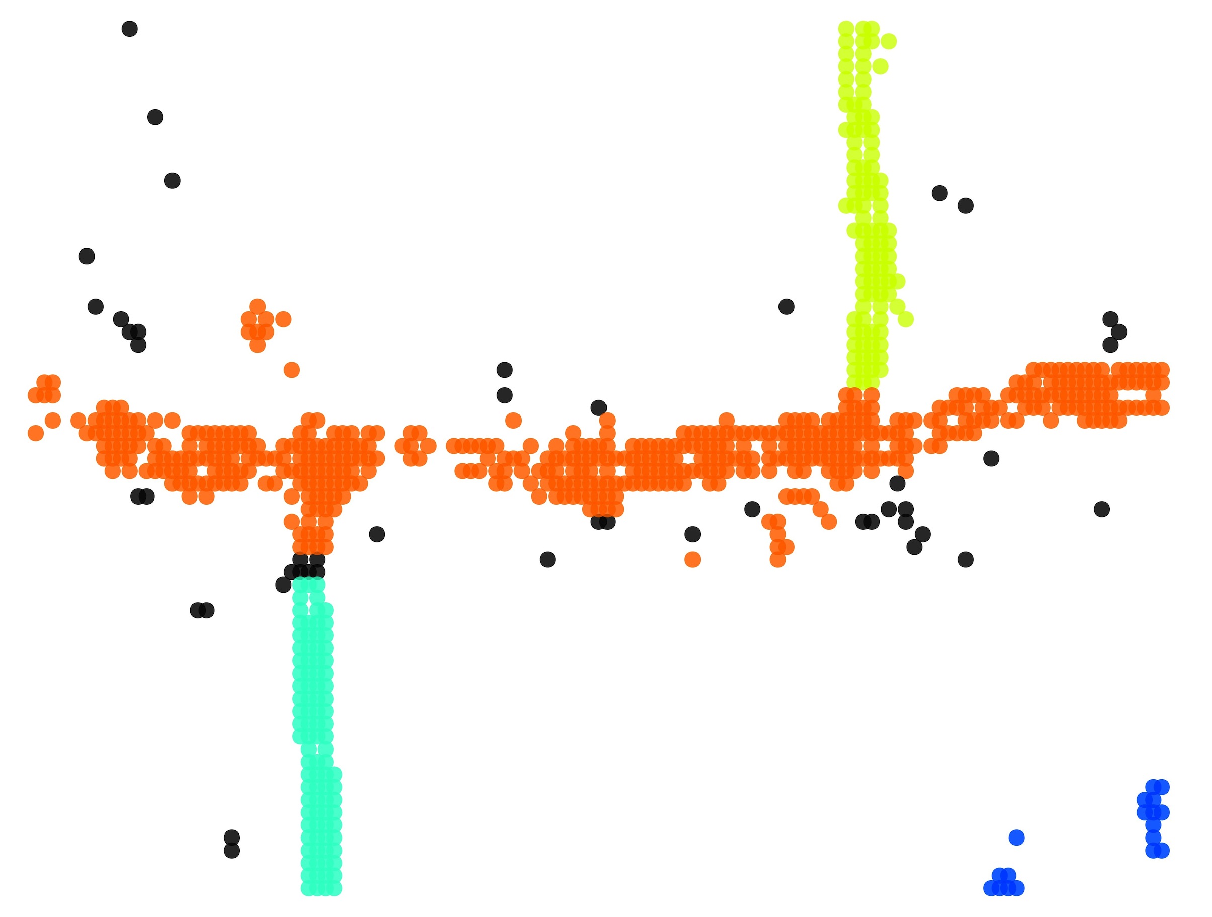
(a)	(b)	(c)	(d)

Figure 11: (a) original and (b) processed images of floor cracks; (c) and (d) show clustering based on CTFs.

To further test the ability of the method to cluster intersecting manifolds, we experimented with synthetic data comprising multiple arrangements such as the intersecting lines in Fig. 1(b).

Example 13.

We consider three syntehtic datasets of point clouds representing random arrangements of: (i) three line segments in $\mathbb{R}^{2}$; (ii) four curves in $\mathbb{R}^{2}$ that are either line segments or arcs of parabolas; and (iii) three patches of planes in $\mathbb{R}^{3}$. Each of these datasets contains a total of 250 point clouds, 50 used for training the algorithm and 200 test samples. The points in each point cloud are labeled to allow quantification of the accuracy of the output of the algorithm. Fig. 12 shows a few samples from each of these datasets.

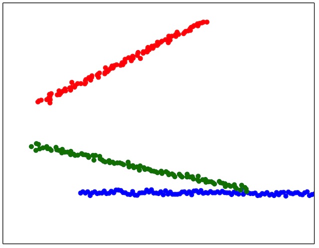
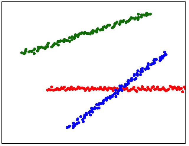
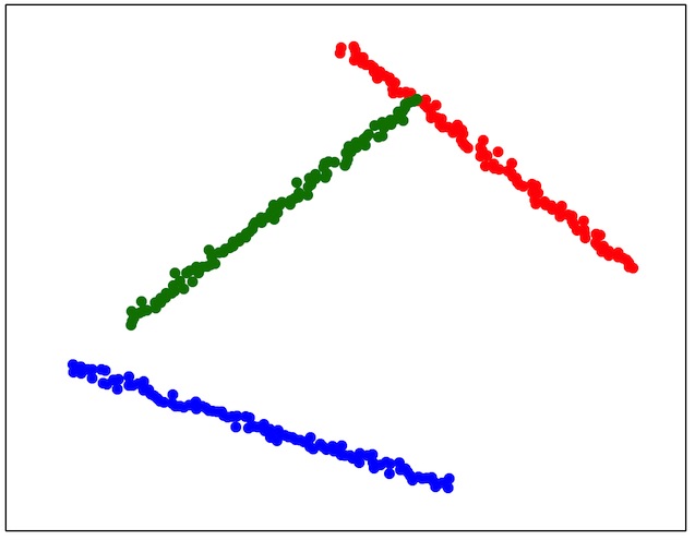
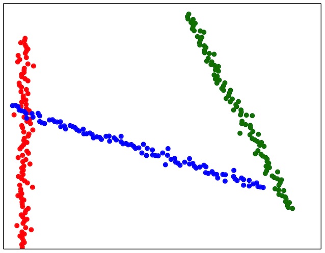
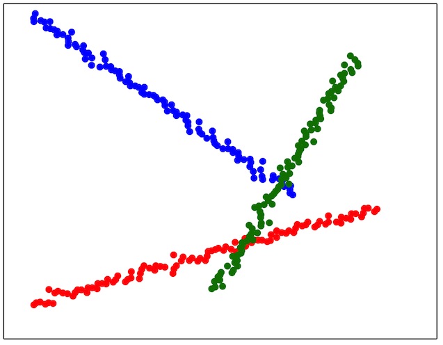
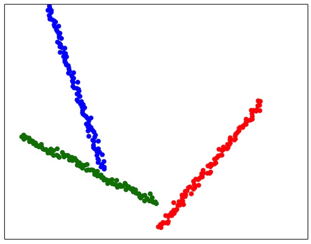
Figure 12: Random arrangements of line segments (row 1), segments of lines and parabolas (row 2), and plane patches (row 3).

Parameter values that optimize classification performance are learned from the training samples. Note, however, that even though the number $k$ of clusters is known, specifying a height $h$ that yields precisely $k$ clusters may yield undesirable results. For example, important clusters representing different components of an arrangement of manifolds may get merged due to the presence of outliers or the behavior near the intersections. Thus, it is often preferable to choose a lower cutoff level before this phenomenon occurs at the expense of getting a larger number $\ell$ of clusters. In such situations, we select the largest $k$ clusters and assign each point in the remaining $(\ell-k)$ clusters to the closest of the top $k$ clusters. Experiments indicate that a good baseline for the cutoff level $h$ is the mean cophenetic distance, which for a point cloud $\{x_{1},\ldots,x_{n}\}\subset\mathbb{R}^{d}$ is given by

$$h_{0}=\frac{2}{n(n-1)}\sum_{i<j}u_{\alpha_{n};\gamma,\sigma}(x_{i},x_{j})\,.$$ (91)

In the learning phase, we typically search for $h$ in a neighborhood of $h_{0}$ whose width is determined by the variance of the distribution of the cophenetic distances.

With the learned parameter values, the algorithm performs well in all three cases. For each point cloud we count the number of misclassified points and calculate the average error (AE) and the mean error (ME) rates over all test samples obtaining:

• arrangements of lines: 9.59% (AE) and 4.17% (ME);

• lines and parabolas: 9.93% (AE) and 3.38% (ME);

• arrangements of planes: 7.00% (AE) and 2.42% (ME).

As expected, a closer inspection of the results reveals that most of the errors occur at points near the intersections of the clusters, where the covariance tensors are not as informative for clustering purposes.

7 Concluding Remarks

We introduced the notion of multiscale covariance tensor fields associated with Euclidean random variables and developed a framework for the systematic study of the shape of data using localized covariance tensors. We investigated foundational questions such as stability and consistency of multiscale CTFs, provided illustrations of how CTFs let us uncover geometry underlying data, and applied the methods to manifold clustering. We also introduced multiscale Fréchet functions, which are scalar fields derived from CTFs that fully capture the distributions of random vectors. Multiscale Fréchet functions are particularly well suited for extension of the methods of this paper to non-Euclidean random variables, a problem that is receiving ever increasing attention in data science. In this setting, the goal is to devise methods that can cope with random variables taking values in spaces such as Riemannian manifolds and more general metric spaces. Unless restrictive assumptions are imposed on the sample space and the distributions, CTFs may be difficult to define in this nonlinear realm. In contrast, the Fréchet function formulation can be easily extended to metric spaces supporting a diffusion kernel [42]. In forthcoming work, we will investigate theoretical and computational aspects of such extensions, including the accessibility of information residing in multiscale Fréchet functions, a problem that poses computational challenges even in the case of high-dimensional Euclidean random variables.

In this paper, we only considered radial basis kernels; however, many results extend easily to more general kernels. We emphasized the multiscale formulation largely because of the questions that motivated this work. Nevertheless, the majority of the results apply to kernels that are not scale dependent.

Covariance tensor fields also suggest ways of formalizing the notion of shape of Euclidean data and probability measures. For example, for a distribution $\alpha$ with the property that the covariance tensor field $\Sigma_{\alpha}(\cdot,\sigma)$ associated with a smooth kernel (such as the Gaussian kernel) is non-singular for every $x\in\mathbb{R}^{d}$, $\Sigma_{\alpha}^{-1}(\cdot,\sigma)$ defines a metric tensor with close ties to $\alpha$. This poses the problem of uncovering relationships between Riemannian metrics derived from CTFs, such as $\Sigma_{\alpha}^{-1}(\cdot,\sigma)$, and the shape of $\alpha$.

In a different direction, for a fixed point $x\in\mathbb{R}^{d}$, an interesting problem is that of capturing the values of $\sigma$ for which $\Sigma_{\alpha}(x,\sigma)$ exhibits a “jump” in behavior. This study, in the context of images, gives rise to notions of local scales. Knowledge of local scales for each point $x$ leads to criteria for selecting important, salient points in the spirit of SIFT [43, 2]. The concept of local scales arose first in the context of images [44] and was later extended to probabilty distributions [45]. The notions of local scales in [44, 45] were isotropic. Thus, future developments related to characterizing shape using CTFs are suggested by the possibility of constructing notions of local scales on general shapes [45, 2] which —by exploiting the tensorial nature of $\Sigma_{\alpha}(x,\sigma)$— become sensitive to direction.

Data Accessibility

The synthetic data used in the manifold clustering experiments is available at https://bitbucket.org/diegodiaz-math/ctf-files/.

References

- [1] A. Little, Y.-M. Jung, M. Maggioni, Estimation of intrinsic dimensionality of samples from noisy low-dimensional manifolds in high dimensions with multiscale SVD, in: IEEE/SP 15th Workshop on Statistical Signal Processing, 2009, pp. 85–88.
- [2] D. Díaz Martínez, F. Mémoli, W. Mio, Multiscale covariance fields, local scales, and shape transforms, in: F. Nielsen, F. Barbaresco (Eds.), Geometric Science of Information, Vol. 8085 of Lecture Notes in Computer Science, Springer, 2013, pp. 794–801.
- [3] C. Villani, Topics in Optimal Transportation, Vol. 58 of Graduate Studies in Mathematics, American Mathematical Society, Providence, RI, 2003.
- [4] C. Villani, Optimal Transport, Old and New, Springer, 2009.
- [5] N. Fournier, A. Guillin, On the rate of convergence in Wasserstein distance of the empirical measure, Probability Theory and Related Fields.
- [6] N. García-Trillos, D. Slepčev, On the rate of convergence of empirical measures in -transportation distance, Canadian Journal of Mathematics, doi:10.4153/CJM-2014-044-6.
- [7] W. Allard, G. Chen, M. Maggioni, Multi-scale geometric methods for data sets II: Geometric multi-resolution analysis, Appl Comput Harmonic Anal 32 (2012) 435–462.
- [8] J. Berkmann, T. Caelli, Computation of surface geometry and segmentation using covariance techniques, IEEE Trans Pattern Anal Mach Intell 16 (1994) 1114–1116.
- [9] R. Rusu, Semantic 3D object maps for everyday manipulation in human living environments, Ph.D. thesis, Technische Universität München (2009).
- [10] G. Medioni, M.-S. Lee, C.-H. Tang, A Computational Framework for Segmentation and Grouping, Elsevier Science, 2000.
- [11] T. Brox, B. Rosenhahn, D. Cremers, H.-P. Seidel, Nonparametric density estimation with adaptive, anisotropic kernels for human motion tracking, in: Human Motion – Understanding, Modeling, Capture and Animation, Vol. 4814 of Lecture Notes in Computer Science, Springer, 2007, pp. 152–165.
- [12] D. Kushnir, M. Galun, A. Brandt, Fast multiscale clustering and manifold identification, Pattern Recognition 39 (10) (2006) 1876–1891.
- [13] A. B. Goldberg, X. Zhu, A. Singh, Z. Xu, R. D. Nowak, Multi-manifold semi-supervised learning., in: AISTATS, 2009, pp. 169–176.
- [14] D. Gong, X. Zhao, G. Medioni, Robust multiple manifolds structure learning, arXiv preprint arXiv:1206.4624.
- [15] Y. Wang, Y. Jiang, Y. Wu, Z.-H. Zhou, Spectral clustering on multiple manifolds, IEEE Transactions on Neural Networks 22 (7) (2011) 1149–1161.
- [16] E. Arias-Castro, Clustering based on pairwise distances when the data is of mixed dimensions, IEEE Transactions on Information Theory 57 (3) (2011) 1692–1706.
- [17] E. Arias-Castro, G. Chen, G. Lerman, et al., Spectral clustering based on local linear approximations, Electronic Journal of Statistics 5 (2011) 1537–1587.
- [18] E. Arias-Castro, G. Lerman, T. Zhang, Spectral clustering based on local pca, arXiv preprint arXiv:1301.2007.
- [19] R. Vidal, Y. Ma, S. Sastry, Generalized principal component analysis (GPCA), IEEE Trans Pattern Anal Mach Intell 27 (12) (2005) 1945–1959.
- [20] V. Govind, A tensor decomposition for geometric grouping and segmentation, in: IEEE Conference on Computer Vision and Pattern Recognition, Vol. 1, 2005, pp. 1150–1157.
- [21] G. Chen, G. Lerman, Spectral curvature clustering (SCC), Int J Comput Vis 81 (3) (2009) 317–330.
- [22] G. Lerman, T. Zhang, Robust recovery of multiple subspaces by geometric minimization, Ann Stat 39 (5) (2011) 2686–2715.
- [23] T. Zhang, A. Szlam, Y. Wang, G. Lerman, Hybrid linear modeling via local best-fit flats, Int J Comput Vis 100 (3) (2012) 217–240.
- [24] G. Liu, Z. Lin, S. Yan, J. Sun, Y. Ma, Robust recovery of subspace structures by low-rank representation, IEEE Trans Pattern Anal Mach Intell 35 (1) (2013) 171–184.
- [25] E. Elhamifar, R. Vidal, Sparse subspace clustering: algorithm, theory, and applications, IEEE Trans Pattern Anal Mach Intell 35 (11) (2013) 2765–2781.
- [26] M. Soltanolkotabi, E. Elhamifar, E. J. Candes, et al., Robust subspace clustering, The Annals of Statistics 42 (2) (2014) 669–699.
- [27] M. Polito, P. Perona, Grouping and dimensionality reduction by locally linear embedding, in: NIPS, 2001, pp. 1255–1262.
- [28] A. Gionis, A. Hinneburg, S. Papadimitriou, P. Tsaparas, Dimension induced clustering, in: Proceedings of the eleventh ACM SIGKDD international conference on Knowledge discovery in data mining, ACM, 2005, pp. 51–60.
- [29] R. Souvenir, R. Pless, Manifold clustering, in: International Conference on Computer Vision, 2005, pp. 648–653.
- [30] G. Haro, G. Randall, G. Sapiro, Stratification learning: Detecting mixed density and dimensionality in high dimensional point clouds, in: NIPS, 2006, pp. 553–560.
- [31] X. Wang, K. Slavakis, G. Lerman, Riemannian multi-manifold modeling, arXiv preprint arXiv:1410.0095.
- [32] G. Carlsson, F. Mémoli, Characterization, stability and convergence of hierarchical clustering methods, J Mach Learn Res 11 (2010) 1425–1470.
- [33] J. Bruce, P. Giblin, Curves and singularities: a geometrical introduction to singularity theory, Cambridge University Press, 1992.
- [34] C. Givens, R. Shortt, A class of Wasserstein metrics for probability distributions, Michigan Math J 31 (2) (1984) 231–240.
- [35] R. M. Dudley, Real Analysis and Probability in Cambridge Studies in Advanced Mathematics, Vol. 74, Cambridge University Press, Cambridge, England, 2002.
- [36] A. Jain, R. Dubes, Algorithms for Clustering Data, Prentice Hall, Englewood Cliffs, NJ, 1988.
- [37] R. Tron, R. Vidal, A benchmark for the comparison of 3-D motion segmentation algorithms, in: IEEE Conference on Computer Vision and Pattern Recognition, 2007, pp. 1–8.
- [38] G. Chen, G. Lerman, Foundations of a multi-way spectral clustering framework for hybrid linear modeling, Foundations of Computational Mathematics 9 (5) (2009) 517–558.
- [39] R. Sibson, SLINK: an optimally efficient algorithm for the single-link cluster method, Comp J 16 (1) (1973) 30–34.
- [40] D. Burago, Y. Burago, S. Ivanov, A Course in Metric Geometry, Graduate Studies in Mathematics, American Mathematical Society, Providence, RI, 2001.
- [41] F. Mémoli, Gromov-Wasserstein distances and the metric approach to object matching, Foundations of Computational Mathematics (2011) 1–71.
- [42] R. Coifman, S. Lafon, Diffusion maps, Appl Comput Harmonic Anal 21 (1) (2006) 5–30.
- [43] D. G. Lowe, Distinctive image features from scale-invariant keypoints, International Journal of Computer Vision 60 (2) (2004) 91–110.
- [44] P. W. Jones, T. M. Le, Local scales and multiscale image decompositions, Applied and Computational Harmonic Analysis 26 (3) (2009) 371–394.
- [45] T. Le, F. Mémoli, Local scales on curves and surfaces, Applied and Computational Harmonic Analysis 33 (3) (2012) 401 – 437.