Three-step implementation of any $n\!\times\!n$ unitary with a complete graph of $n$ qubits

Abstract

Quantum computation with a complete graph of superconducting qubits has been recently proposed, and applications to amplitude amplification, phase estimation, and the simulation of realistic atomic collisions given $[{\rm Phys.~{}Rev.~{}A}\ {\bf 91},062309\,(2015)]$. This single-excitation subspace (SES) approach does not require error correction and is practical now. Previously it was shown how to implement symmetric $n\!\times\!n$ unitaries in a single step, but not general unitaries. Here we show that any element in the unitary group ${\rm U}(n)$ can be executed in no more than three steps, for any $n$. This enables the implementation of highly complex operations in constant time, and in some cases even allows for the compilation of an entire algorithm down to only three operations. Using this protocol we show how to prepare any pure state of an SES chip in three steps, and also how to compute, for a given SES state $\rho,$ the expectation value ${\rm Tr}(\rho O)$ of any $n\!\times\!n$ Hermitian observable $O$ in a constant number of steps.

I PRETHRESHOLD QUANTUM COMPUTATION

There is currently great interest in the development of special-purpose quantum computing devices and methodologies that do not require full error correction and which are practical now. For example, D-Wave Systems produces commercial quantum annealers based on superconducting circuits that solve an important class of binary optimization problems Johnson et al. (2011). However it is not known whether the D-Wave annealers can outperform conventional classical supercomputers Boixo et al. (2014); Ronnow et al. (2014). An optical approach Aaronson and Arkhipov (2013) that solves an arguably less important problem—sampling from the distribution of bosons scattered by a unitary network—but which is likely capable of quantum speedup has also been investigated Broome et al. (2013); Spring et al. (2013); Tillmann et al. (2013). An approach called the single-excitation-subspace (SES) method, also based on supercondonducting circuits, has been proposed [Geller et al., 2015]. Here computations are performed in the $n$-dimensional SES of a complete graph of $n$ qubits. We call these examples prethreshold, referring to the threshold theorem of fault-tolerant quantum computation, because they do not require exceeding fidelity and qubit-number thresholds before being applicable.

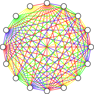
Figure 1: (Color online) Complete graph with $n\!=\!16$. The vertices (open circles) are qubits and the edges (colored lines) are tunable couplers.

A quantum computer chip implementing the SES method consists of a fully connected array of superconducting qubits with tunable frequencies and tunable pairwise $\sigma^{x}\!\otimes\sigma^{x}$ couplings; an abstract representation is given in Fig. 1. It works by operating in a subspace of the full $2^{n}$-dimensional Hilbert space where the Hamiltonian can be directly programmed. This programmability eliminates the need to decompose operations into elementary one- and two-qubit gates, enabling larger computations to be performed within the available coherence time. The price for this high degree of controllability is that the approach is not scalable. However, a technically unscalable quantum computer is still useful for prethreshold quantum computation and might even be able to achieve speedup relative to a classical supercomputer for certain tasks. The SES approach trades physical qubits and high connectivity for, in effect, longer coherence. This is a sensible trade for quantum computing architectures such as superconducting circuits, whose largest prethreshold problem sizes are limited by coherence time, not by the difficulty of introducing additional qubits. A realistic chip layout that provides space for the coupler circuits and avoids the crossovers of Fig. 1 is shown in Fig. 2.

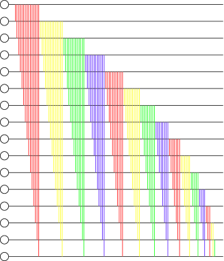
Figure 2: (Color online) Possible layout for the 16-qubit chip.

II CONTENT OF THIS PAPER

A significant restriction of the SES method presented in Ref. Geller et al. (2015) is that the Hamiltonian programmed into the hardware is real and symmetric, whereas the most general Hamiltonian is complex Hermitian. If a target operation has the form $e^{-iA},$ where $A$ is a known real symmetric generator matrix, then the unitary can be implemented in one step. This is the case when the unitary is symmetric ($U=U^{\top}$) and is reviewed in Sec. III.1. In that section we also provide an improved procedure for constructing the time-optimal SES Hamiltonian ${\cal H}$ corresponding to a given generator $A$.

However, a general element of the unitary group ${\rm U}(n)$ has the form $e^{-iM}$ with $M$ complex Hermitian. This is the nonsymmetric unitary case ($U\neq U^{\top}$) discussed in Sec. III.2. We show there that any nonsymmetric element $U\in{\rm U}(n)$ can be implemented in three steps, for any $n$.

Applications of these techniques are given in Sec. IV. In Sec. IV.1 we show how to simulate time-independent but otherwise arbitrary $n\!\times\!n$ complex Hamiltonians with an SES chip in three steps. In Sec. IV.2 we show how to prepare pure but otherwise arbitrary SES states in three steps. And in Sec. IV.3 we explain how to compute expectation values of arbitrary $n\!\times\!n$ Hermitian observables.

III SES IMPLEMENTATION OF UNITARY OPERATORS

III.1 Single-step implementation of symmetric unitaries

The basic single-step operation in SES quantum computing is the implementation of symmetric unitaries of the form $U=e^{-iA}$, with $A$ real and symmetric Geller et al. (2015). Therefore, a standard task in SES algorithm design and implementation is the construction of an optimal protocol—an SES Hamiltonian ${\cal H}$ and evolution time $t_{\rm qc}$—to implement that unitary. We assume here that the generator matrix $A$ is known; if it is not then the classical overhead for obtaining $A$ from $U$ must be included in the quantum runtime. (We also note that the generator $A=i\log U$ is not unique.) The optimal protocol for implementing a symmetric unitary depends on the functionality assumed of the chip, especially of the tunable coupler circuits. Here we assume that the experimentally controlled SES Hamiltonian can be written, apart from an additive constant, as

$${\cal H}=g_{\rm max}K\ \ \ {\rm with}\ \ \ -1\leq K_{ii^{\prime}}\leq 1,$$ (1)

which we call the standard form. In this case we are assuming that the couplings can be tuned continuously between $-g_{\rm max}$ and $g_{\rm max}$, and that the qubit frequencies can be varied within a window of width $2g_{\rm max}$ about some parking frequency. Because we are free to change the overall phase of an SES state, we write the symmetric unitary as

$$U=e^{-i(A-cI)}e^{-ic},$$ (2)

where $I$ is the $n\!\times\!n$ identity matrix, and then ignore the global phase $e^{-ic}$. The value of $c$ is chosen to minimize the evolution time $t_{\rm qc}$, which is proportional to the angle

$$\theta_{\!A}\equiv\max_{ii^{\prime}}|A_{ii^{\prime}}-c\delta_{ii^{\prime}}|.$$ (3)

The $K$ matrix in (1) is then given by

$$K=\frac{A-cI}{\theta_{\!A}},$$ (4)

and the evolution time is

$$t_{\rm qc}=\frac{\hbar\theta_{\!A}}{g_{\rm max}}.$$ (5)

Note that $\theta_{\!A}$ is not bounded by $2\pi$ and can become arbitrarily large. The global phase angle that minimizes $\theta_{\!A}$ is

$$c=\frac{\min_{i}A_{ii}+\max_{i}A_{ii}}{2},$$ (6)

which is proved below. Although we have assumed that the SES Hamiltonian ${\cal H}=g_{\rm max}K$ is abruptly switched on for a time $t_{\rm qc}$ before being abruptly switched off—which is the fastest protocol—any SES Hamiltonian of the form ${\cal H}=g(t)K$ such that $\int(g/\hbar)\,dt=\theta_{\!A}$ may be used instead.

To minimize (3) over $c$ we consider two cases: In the first case $\max_{ii^{\prime}}|A_{ii^{\prime}}|$ occurs for an off-diagonal element of $A$, in which case the minimum value of $\theta_{\!A}$ is independent of $c$ (because $c$ only affects the diagonal elements of the shifted matrix $A-cI$). Therefore we only need to consider the second case where $\max_{ii^{\prime}}|A_{ii^{\prime}}|$ occurs for a diagonal element. The diagonal elements consist of points

$$x\in\big{\{}A_{11},A_{22},\cdots,A_{nn}\big{\}}$$ (7)

on the real number line, bounded between $\min_{i}A_{ii}$ and $\max_{i}A_{ii}$. Placing $c$ at the midpoint of the smallest region containing all the points in (7) minimizes the largest distance $|A_{ii}-c|.$

III.2 Three-step implementation of nonsymmetric unitaries: ABA decomposition

Our protocol relies on the matrix decomposition

$$U=O_{1}e^{-iD}O_{2}^{\top},$$ (8)

where $D$ is a real diagonal matrix and the $O_{i}\in O(n)$ are real orthogonal matrices. This identity follows from the $KAK$ decomposition of the Lie group ${\rm U}(n)\!$ Knapp (1996). To obtain the $O_{i}$ and $D$ from $U$, we first compute

$$\chi\equiv UU^{\top}=O_{1}e^{-2iD}O_{1}^{\top},$$ (9)

which is both symmetric and unitary. The real and imaginary parts of $\chi$ are also separately symmetric. Then the unitarity condition

$$\big{(}{\rm Re}\,\chi-i\,{\rm Im}\,\chi\big{)}\big{(}{\rm Re}\,\chi+i\,{\rm Im}\,\chi\big{)}=I$$ (10)

shows that ${\rm Re}\,\chi$ and ${\rm Im}\,\chi$ commute and can be simultaneously diagonalized. $O_{1}$ is determined by a Schur decomposition of ${\rm Re}\,\chi$, which always produces a real $O_{1}$ (unlike the decomposition of $\chi$ itself). Then $e^{-2iD}$ and $O_{2}$ are obtained from $O_{1}^{\top}\chi O_{1}$ and $U^{\top}O_{1}e^{iD}\!,$ respectively.

The three-step implementation for a nonsymmetric $U\in{\rm U}(n)$ follows from the identity

$$U=e^{-iA}e^{-iB}e^{iA},$$ (11)

which we call the ABA decomposition. Here $A$ and $B$ are real symmetric $n\!\times\!n$ matrices. To derive (11) we express the target unitary in the spectral form $U=Ve^{-i\Lambda}V^{\dagger},$ where $V$ is complex unitary and $\Lambda$ is real and diagonal. Decomposing $V$ using (8) we have

$$U = O_{1}e^{-iD}O_{2}^{\top}e^{-i\Lambda}O_{2}\,e^{iD}O_{1}^{\top},$$ (12)

$$= e^{-iO_{1}DO_{1}^{\top}}(O_{1}O_{2}^{\top})\,e^{-i\Lambda}\,(O_{1}O_{2}^{\top})^{\!\top}e^{iO_{1}DO_{1}^{\top}},$$

which leads to (11) with generators

$$A = O_{1}DO_{1}^{\top},$$ (13)

$$B = O_{1}O_{2}^{\top}\Lambda O_{2}O_{1}^{\top},$$ (14)

which are both real and symmetric. The classical runtime to obtain $A$ and $B$ is about

$$1.4\!\times\!n^{2.3}\,{\rm\mu s}$$ (15)

on a laptop computer com . The quantum runtime to implement a nonsymmetric unitary is

$$t_{\rm qc}=\frac{\hbar(2\theta_{\!A}+\theta_{\!B})}{g_{\rm max}},$$ (16)

with $\theta$ defined in (3). The generator matrices $A$ and $B$ in (11) are not unique.

The ABA decomposition allows for the possibility of implementing highly complex operations in three steps. But this does not imply that an entire algorithm, compiled into a single unitary, can be implemented in constant time, because the compiled unitary might not be known a priori, and there is classical overhead (15) for computing $A$ and $B$. More importantly, evaluating $A$ and $B$ for an entire algorithm would presumably be prohibitive when one is attempting to outperform classical computers. Furthermore, algorithms might include measurement steps that cannot be postponed to the end.

IV APPLICATIONS

IV.1 Hamiltonian simulation

A useful application of (11) is to $U=e^{-iHt/\hbar},$ where $H$ is a given complex Hamiltonian. In this case we have

$$e^{-iHt/\hbar}=e^{-iA}e^{-iB}e^{iA},$$ (17)

with $A$ and $B$ given by (13) and (14), where $\Lambda$ is a diagonal matrix containing $t/\hbar$ times the spectrum of $H$. This enables the fast simulation of any time-independent Hamiltonian with an SES chip tim .

IV.2 SES pure state preparation in 3 steps

In some cases it is possible to compile an entire algorithm down to only three steps. As an example we give an algorithm for preparing any (normalized) pure SES state of the form

$$|\psi\rangle=\sum_{i=1}^{n}a_{i}\,|i),\ \ \ \ a_{i}=|a_{i}|e^{i\theta_{i}},\ \ \ \ 0\leq\theta_{i}<2\pi.$$ (18)

Here $|i)\equiv|0\cdots 1_{i}\cdots 0\rangle$ is the $i$th SES basis state of the $n$-qubit processor. We proceed by giving a protocol with linear depth that is practical for small $n$, which is then subsequently compiled down to three steps.

We start with the basis state $|1)$, which is prepared from the system ground state $|00\cdots 0\rangle$ by a microwave pulse, and then apply the standard-form SES Hamiltonian ${\cal H}=g_{\rm max}K_{\rm star}$ for a time $t_{\rm qc}=\pi\hbar/\sqrt{n}g_{\rm max},$ with

$$K_{\rm star}\equiv\begin{pmatrix}1&\frac{1}{2}&\frac{1}{2}&\cdots&\frac{1}{2}\\ \frac{1}{2}&0&0&\cdots&0\\ \frac{1}{2}&0&0&\cdots&0\\ \vdots&\vdots&\vdots&\ddots&\vdots\\ \frac{1}{2}&0&0&\cdots&0\\ \end{pmatrix}$$ (19)

the adjacency matrix for a star graph with qubit 1 at the center (see Sec. IIIA of Ref. [Geller et al., 2015]). This produces the uniform state

$$\big{|}{\rm unif}\big{\rangle}\equiv\frac{|1)+|2)+\cdots+|n)}{\sqrt{n}},$$ (20)

apart from a phase.

If the occupation probabilities in the target state (18) are uniform,

$$|a_{i}|^{2}=\frac{1}{n},$$ (21)

we call it a uniform weight state and represent it by the bar graph in Fig. 3. In this case we would apply the diagonal Hamiltonian ${\cal H}=g_{\rm max}K$, where

$$K=-\begin{pmatrix}\frac{\theta_{1}}{2\pi}&0&\cdots&0\\ 0&\frac{\theta_{2}}{2\pi}&\cdots&0\\ \vdots&\vdots&\ddots&\vdots\\ 0&0&\cdots&\frac{\theta_{n}}{2\pi}\\ \end{pmatrix}$$ (22)

to the uniform state $|{\rm unif}\rangle$ for a time $t_{\rm qc}=2\pi\hbar/g_{\rm max},$ which gives the desired target.

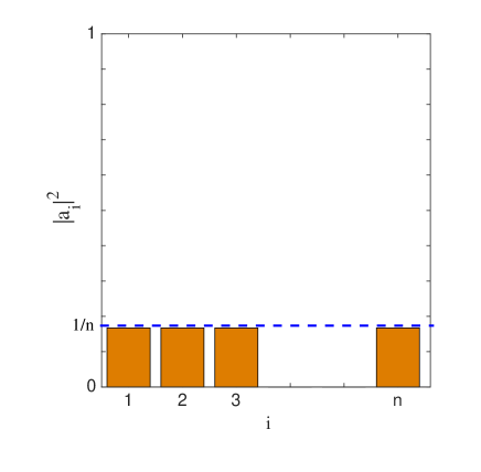
Figure 3: (color online) Occupation probabilities for a uniform weight state. Phases of the probability amplitudes $a_{i}$ are not represented in this figure.

Typically the target is not a uniform weight state, as represented in Fig. 4. In this case we use the solution

$$|{\rm unif}\rangle=W_{\rm diag}\,(U_{\rm swap}U_{\rm diag})_{M}\!\cdots(U_{\rm swap}U_{\rm diag})_{1}|\psi\rangle$$ (23)

to the inverse problem of constructing the uniform state $|{\rm unif}\rangle$ from the target Law and Eberly (1996); Hofheinz et al. (2009). Each of the $M$ steps in (23) consists of a pair of operations $U_{\rm diag}$ and $U_{\rm swap}$ that move weight between a pair of components. After $M=O(n)$ steps a uniform weight state is created. The final operation $W_{\rm diag}$ shifts the phases of the uniform weight state to that of (20). The first step is:

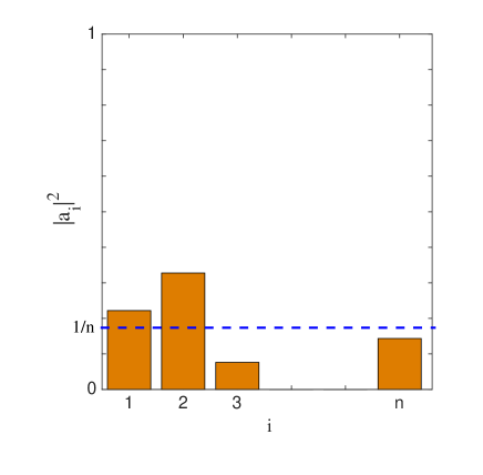
Figure 4: (color online) Occupation probabilities for a typical target state. In this example the components of maximum and minimum weight have indices $i_{\rm max}\!=\!2$ and $i_{\rm min}\!=\!3$.

1. Find the components $i_{\rm min}$ and $i_{\rm max}$ with the smallest and largest weights, respectively (if not unique, any solution is sufficient). These satisfy

   $$|a_{i_{\rm min}}|^{2}\leq\frac{1}{n}\leq|a_{i_{\rm max}}|^{2},$$ (24)

   excluding the case where both $\leq$ signs are identities (which would violate the assumption that the target is nonuniform). Therefore $|a_{i_{\rm min}}|^{2}<|a_{i_{\rm max}}|^{2}\!.$

2. Perform a phase shift $U_{\rm diag}=e^{-i{\cal H}t_{\rm qc}/\hbar}$ that brings the probability amplitudes $a_{i_{\rm min}}$ and $a_{i_{\rm max}}$ to the form $a_{i_{\rm min}}=|a_{i_{\rm min}}|$ and $a_{i_{\rm max}}=i|a_{i_{\rm max}}|,$ with $|a_{i_{\rm min}}|<|a_{i_{\rm max}}|$. Apply SES Hamiltonian (1), where $K$ is a diagonal matrix with $K_{i_{\rm min},i_{\rm min}}=\theta_{i_{\rm min}}/3\pi$ and $K_{i_{\rm max},i_{\rm max}}=(\theta_{i_{\rm max}}/3\pi)-\frac{1}{6}$, the other elements zero, and $t_{\rm qc}=3\pi\hbar/g_{\rm max}.$ This phase shift is necessary to prepare the state for the next operation.

3. Implement a partial iSWAP $U_{\rm swap}=e^{-i{\cal H}t_{\rm qc}/\hbar}$ from component $i_{\rm max}$ to $i_{\rm min}$ to bring the weight of $i_{\rm min}$ to the uniform value,

   $$|a_{i_{\rm min}}|^{2}\rightarrow\frac{1}{n},$$ (25)

   and leaving component $i_{\rm max}$ with weight

   $$|a_{i_{\rm max}}|^{2}\rightarrow|a_{i_{\rm min}}|^{2}+|a_{i_{\rm max}}|^{2}-\frac{1}{n}.$$ (26)

   Apply SES Hamiltonian (1) with $K_{i_{\rm min},i_{\rm max}}\!=\!K_{i_{\rm max},i_{\rm min}}\!=\!1$ and all other elements zero, and $t_{\rm qc}=\varphi\hbar/g_{\rm max}$ with $\varphi$ given by

   $$|a_{i_{\rm min}}|\cos\varphi+|a_{i_{\rm max}}|\sin\varphi=\sqrt{1/n}.$$ (27)

   There is always a solution with $0\!<\!\varphi\!<\!\pi/2$.

This completes the first step.

If after the first step $(U_{\rm swap}U_{\rm diag})_{1}|\psi\rangle$ is a uniform weight state, it can be written in the form

$$\frac{e^{i\alpha_{1}}|1)+e^{i\alpha_{2}}|2)+\cdots+e^{i\alpha_{n}}|n)}{\sqrt{n}},$$ (28)

and we apply the final operation $W_{\rm diag}=e^{-i{\cal H}t_{\rm qc}/\hbar}$ to produce (20). Here we use SES Hamiltonian (1) with

$$K=\begin{pmatrix}\frac{\alpha_{1}}{2\pi}&0&\cdots&0\\ 0&\frac{\alpha_{2}}{2\pi}&\cdots&0\\ \vdots&\vdots&\ddots&\vdots\\ 0&0&\cdots&\frac{\alpha_{n}}{2\pi}\\ \end{pmatrix}$$ (29)

and $t_{\rm qc}=2\pi\hbar/g_{\rm max}.$ If $(U_{\rm swap}U_{\rm diag})_{1}|\psi\rangle$ is not a uniform weight state, we again find the minimum and maximum weight components $i_{\rm min}$ and $i_{\rm max}$, and follow the above protocol to generate $(U_{\rm swap}U_{\rm diag})_{2}(U_{\rm swap}U_{\rm diag})_{1}|\psi\rangle.$ The procedure is repeated until

$$(U_{\rm swap}U_{\rm diag})_{M}\cdots(U_{\rm swap}U_{\rm diag})_{2}(U_{\rm swap}U_{\rm diag})_{1}|\psi\rangle$$ (30)

is a uniform weight state, after which $W_{\rm diag}$ is applied. The number of iterations required satisfies

$$M\leq n-1.$$ (31)

This completes the solution to the inverse problem (23).

We now use (23) to obtain

$$|\psi\rangle=(U_{\rm diag}^{\dagger}U_{\rm swap}^{\dagger})_{1}\cdots(U_{\rm diag}^{\dagger}U_{\rm swap}^{\dagger})_{M}\,W_{\rm diag}^{\dagger}|{\rm unif}\rangle,$$ (32)

which solves the general state-preparation problem in $O(n)$ steps. Hermitian conjugations are implemented by changing the signs of the $K$ matrices given above. The protocol given in (32) is, by itself, practical for small $n$.

The complete state preparation operation can be summarized as

$$|\psi\rangle=U\,|1),$$ (33)

where

$$U\equiv(U_{\rm diag}^{\dagger}U_{\rm swap}^{\dagger})_{1}\cdots(U_{\rm diag}^{\dagger}U_{\rm swap}^{\dagger})_{M}\,W_{\rm diag}^{\dagger}\,e^{-i\frac{\pi}{\sqrt{n}}K_{\rm star}}$$ (34)

is the compiled unitary of the state-preparation algorithm. The three-step state preparation protocol uses the ABA decomposition to implement (34). The total state preparation time, not including the $|1)$ state initialization time, is given in (16).

For example, suppose we wish to prepare the randomly chosen target

$$|\psi\rangle\!=\!0.4829\,|1)+(-0.5478\!-\!0.0575i)\,|2)+(0.1142\!+\!0.2387i)\,|3)$$

$$+(0.4095\!+\!0.2400i)\,|4)+(-0.3215\!+\!0.2545i)\,|5),$$ (35)

in the $n\!=\!5$ graph, where for convenience the first component has been chosen to be real. Following the state-preparation protocol leads to the compiled unitary

$$U=\begin{pmatrix}0.4829&0.4499-0.0158i&0.4499-0.0158i&0.4478-0.0133i&0.3984+0.0450i\\ -0.5478-0.0575i&0.5855-0.4153i&0.1778-0.0249i&-0.1305+0.2703i&-0.0855+0.2273i\\ 0.1142+0.2387i&0.4664+0.0700i&-0.7862-0.2582i&0.0910-0.0284i&0.1145-0.0222i\\ 0.4095+0.2400i&0.0841-0.1271i&0.1471-0.1492i&-0.7941+0.1818i&0.1471-0.1492i\\ -0.3215+0.2545i&0.1071+0.1577i&0.1071+0.1577i&0.1071+0.1580i&0.1399-0.8386i\\ \end{pmatrix},$$ (36)

up to a phase factor. The first column of (36) is the target state. The ABA decomposition (11) then leads to

$$A\!=\!\begin{pmatrix}-1.1145&0.1981&0.3247&-0.0776&-0.1888\\ 0.1981&-2.6988&0.0219&-0.2069&-0.0249\\ 0.3247&0.0219&-1.9798&-0.5623&0.1052\\ -0.0776&-0.2069&-0.5623&-0.5291&-0.0747\\ -0.1888&-0.0249&0.1052&-0.0747&-1.7104\\ \end{pmatrix}$$ (37)

and

$$B\!=\!\begin{pmatrix}-3.0826&1.8972&0.3983&0.8753&0.5934\\ 1.8972&-3.7784&0.5761&0.3537&0.5581\\ 0.3983&0.5761&-3.2370&0.1664&0.2327\\ 0.8753&0.3537&0.1664&-2.6191&0.1488\\ 0.5934&0.5581&0.2327&0.1488&-4.6171\\ \end{pmatrix}.$$ (38)

The associated $K$ matrices and evolution times are determined from the procedure given in Sec. III.1:

$$K_{A} \!=\! \begin{pmatrix}0.4604&0.1826&0.2993&-0.0715&-0.1741\\ 0.1826&-1&0.0202&-0.1907&-0.0229\\ 0.2993&0.0202&-0.3373&-0.5183&0.0970\\ -0.0715&-0.1907&-0.5183&1&-0.0689\\ -0.1741&-0.0229&0.0970&-0.0689&-0.0889\\ \end{pmatrix},$$

$$\theta_{A} = 1.0848,$$ (39)

and

$$K_{B} \!=\! \begin{pmatrix}0.2822&1&0.2100&0.4614&0.3128\\ 1&-0.0845&0.3037&0.1864&0.2942\\ 0.2100&0.3037&0.2009&0.0877&0.1226\\ 0.4614&0.1864&0.0877&0.5266&0.0785\\ 0.3128&0.2942&0.1226&0.0785&-0.5266\\ \end{pmatrix},$$

$$\theta_{B} = 1.8972.$$ (40)

The total state preparation time, not counting the $|1)$ state initialization, is given by (16). This is about $13\,{\rm ns}$ for the target state (35) in an SES chip with $g_{\rm max}/2\pi=50\,{\rm MHz}$.

Although state preparation is implemented in three steps for any $n$, the runtime does have a weak $n$-dependence, because $\theta_{\!A}$ and $\theta_{\!B}$ do. Averaged over random targets we find that

$$\overline{2\theta_{\!A}+\theta_{\!B}}\approx 4.0\!\times\!n^{0.06}\!.$$ (41)

For small $n$, either the linear-depth protocol (32) or the three-step protocol based on (34) can be used. However for large $n$, only the three-step protocol is practical.

IV.3 Computation of expectation values

Finally, we show how to compute the expectation value

$$\langle O\rangle\equiv{\rm Tr}(\rho O)$$ (42)

of any $n\!\times\!n$ Hermitian observable $O$, by implementing the protocol of Reck et al. Reck et al. (1994). Here $\rho$ is any pure or mixed SES state provided as an input to the procedure.

Standard readout of an SES processor consists of the simultaneous measurement of each qubit in the diagonal basis. The SES condition means that a single qubit will be found in the state $|1\rangle$, with the remaining $n-1$ qubits in $|0\rangle.$ Let $i$ be the qubit observed in it’s excited state. The probability of observing the excitation in qubit $i$ is $p_{i}=(i|\rho|i)$. Therefore, if we have access to multiple copies of $\rho$ we can repeat the readout $N$ times to obtain estimates of the occupation probabilities $p_{i}$ with sampling errors no larger than $(2\sqrt{N})^{-1}$.

To compute $\langle O\rangle$, perform a (classical) spectral decomposition to a unitary $V$ containing the eigenvectors of $O$ as columns, and a real diagonal matrix $D$: $O=VDV^{\dagger}$. Then we have

$$\langle O\rangle={\rm Tr}(\rho VDV^{\dagger})={\rm Tr}(\rho^{\prime}D),$$ (43)

where

$$\rho^{\prime}\equiv V^{\dagger}\rho V.$$ (44)

Therefore we can compute $\langle O\rangle$ by applying the unitary operator $V^{\dagger}$ using the ABA decomposition, measuring the resulting occupation probabilities, which we denote by $p_{i}^{\,\scriptscriptstyle[V^{\dagger}\!]}$ to indicate the application of $V^{\dagger}$, and then classically evaluating the quantity

$$\langle O\rangle=\sum_{i=1}^{n}D_{ii}\,p_{i}^{\,\scriptscriptstyle[V^{\dagger}\!]}.$$ (45)

V CONCLUSIONS

In this work we have extended the SES method of Ref. Geller et al. (2015) to include a three-step implementation of arbitrary $n\times n$ unitaries. The fast state preparation protocol of Sec. IV.2 should be especially useful for practical quantum computing applications.