\RS@ifundefined

subref \newrefsubname = section  \RS@ifundefinedthmref \newrefthmname = theorem  \RS@ifundefinedlemref \newreflemname = lemma 

Randomized Block Subgradient Methods for Convex Nonsmooth and Stochastic Optimization

Qi Deng
qdeng@ufl.edu
Department of Computer and Information Science and Engineering, University of Florida, FL, 32611
   Guanghui Lan
glan@ise.ufl.edu
Department of Industrial and Systems Engineering, University of Florida, FL, 32611
   Anand Rangarajan11footnotemark: 1
anand@cise.ufl.edu
Abstract

Block coordinate descent methods and stochastic subgradient methods have been extensively studied in optimization and machine learning. By combining randomized block sampling with stochastic subgradient methods based on dual averaging ([22, 36]), we present stochastic block dual averaging (SBDA)—a novel class of block subgradient methods for convex nonsmooth and stochastic optimization. SBDA requires only a block of subgradients and updates blocks of variables and hence has significantly lower iteration cost than traditional subgradient methods. We show that the SBDA-based methods exhibit the optimal convergence rate for convex nonsmooth stochastic optimization. More importantly, we introduce randomized stepsize rules and block sampling schemes that are adaptive to the block structures, which significantly improves the convergence rate w.r.t. the problem parameters. This is in sharp contrast to recent block subgradient methods applied to nonsmooth deterministic or stochastic optimization ([3, 24]). For strongly convex objectives, we propose a new averaging scheme to make the regularized dual averaging method optimal, without having to resort to any accelerated schemes.

1 Introduction

In this paper, we mainly focus on the following convex optimization problem:

$$\min_{x\in X}\phi\left(x\right),$$ (1)

where the feasible set $X$ is embedded in Euclidean space $\mathbb{R}^{N}$ for some integer $N>0$. Letting $N_{1},N_{2},\ldots,N_{n}$ be $n$ positive integers such that $\sum_{i=1}^{n}N_{i}=N$, we assume $X$ can be partitioned as $X=X_{1}\times X_{2}\times\ldots X_{n}$, where each $X_{i}\subseteq\mathbb{R}^{N_{i}}$. We denote $x\in X$, by $x=x^{\left(1\right)}\times x^{\left(2\right)}\ldots\times x^{\left(n\right)}$ where $x^{\left(i\right)}\in X_{i}$. The objective $\phi\left(x\right)$ consists of two parts: $\phi\left(x\right)=f\left(x\right)+\omega\left(x\right)$. We stress that both $f\left(x\right)$ and $\omega\left(x\right)$ can be nonsmooth. $\omega\left(x\right)$ is a convex function with block separable structure: $\omega\left(x\right)=\sum_{i=1}^{n}\omega_{i}\left(x_{i}\right)$, where each $\omega_{i}:X_{i}\rightarrow\mathbb{R}$ is convex and relatively simple. In composite optimization or regularized learning, the term $\omega\left(x\right)$ imposes solutions with certain preferred structures. Common examples of $\omega\left(\cdot\right)$ include the $\ell_{1}$ norm or squared $\ell_{2}$ norm regularizers. $f\left(x\right)$ is a general convex function. In many important statistical learning problems, $f\left(x\right)$ has the form of $f\left(x\right)=\mathbf{E}_{\xi}\left[F\left(x,\xi\right)\right]$, where $F\left(x,\xi\right)$ is a convex loss function of $x\in X$ with $\xi$ representing sampled data. When it is difficult to evaluate $f(x)$ exactly, as in batch learning or sample average approximation (SAA), $f\left(x\right)$ is approximated with finite data. Firstly, a large number of samples $\xi_{1},\xi_{2},\ldots,\xi_{m}$ are drawn, and then $f\left(x\right)$ is approximated by $\tilde{f}\left(x\right)=\frac{1}{m}\sum_{i=1}^{m}F\left(x,\xi_{i}\right)$, with the alternative problem:

$$\min_{x\in X}\tilde{\phi}(x):=\tilde{f}\left(x\right)+\omega\left(x\right).$$ (2)

However, although classic first order methods can provide accurate solutions to (2), the major drawback of these approaches is the poor scalability to large data. First order deterministic methods require full information of the (sub)gradient and scan through the entire dataset many times, which is prohibitive for applications where scalability is paramount. In addition, due to the statistical nature of the problem, solutions with high precision may not even be necessary.

To solve the aforementioned problems, stochastic methods—stochastic (sub)gradient descent (SGD) or block coordinate descent (BCD) have received considerable attention in the machine learning community. Both of them confer new advantages in the trade offs between speed and accuracy. Compared to deterministic and full (sub)gradient methods, they are easier to implement, have much lower computational complexity in each iteration, and often exhibit sufficiently fast convergence while obtaining practically good solutions.

SGD was first studied in [29] in the 1950s, with the emphasis mainly on solving strongly convex problems; specifically it only needs the gradient/subgradient on a few data samples while iteratively updating all the variables. In the approach of online learning or stochastic approximation (SA), SGD directly works on the objective (1), and obtains convergence independent of the sample size. While early work emphasizes asymptotic properties, recent work investigate complexity analysis of convergence. Many works ([21, 13, 33, 26, 6, 2, 8]) investigate the optimal SGD under various conditions. Proximal versions of SGD, which explicitly incorporate the regularizer $\omega\left(x\right)$, have been studied, for example in [15, 4, 5, 36].

The study of BCD also has a long history. BCD was initiated in [18, 19], but the application of BCD to linear systems dates back to even earlier (for example see the Gauss-Seidel method in [7]). It works on the approximated problem (2) and makes progress by reducing the original problem into subproblems using only a single block coordinate of the variable at a time. Recent works [23, 28, 30, 17] study BCD with random sampling (RBCD) and obtain non-asymptotic complexity rates. For the regularized learning problem as in (2), RBCD on the dual formulation has been proposed [31, 11, 32]. Although most of the work on BCD focuses on smooth (composite) objectives, some recent work ([3, 37, 35, 39]) seeks to extend the realm of BCD in various ways. The works in [24, 3] discuss (block) subgradient methods for nonsmooth optimization. Combining the ideas of SGD and BCD, the works in [3, 37, 35, 39, 27] employ sampling of both features and data instances in BCD.

In this paper, we propose a new class of block subgradient methods, namely, stochastic block dual averaging (SBDA), for solving nonsmooth deterministic and stochastic optimization problems. Specifically, SBDA consists of a new dual averaging step incorporating the average of all past (stochastic) block subgradients and variable updates involving only block components. We bring together two strands of research, namely, the dual averaging algorithm (DA) [36, 22] which was studied for nonsmooth optimization and randomized coordinate descent (RCD) [23], employed for smooth deterministic problems. Our main contributions consist of the following:

  • Two types of SBDA have been proposed for different purposes. For regularized learning, we propose SBDA-u which performs uniform random sampling of blocks. For more general nonsmooth learning problems, we propose SBDA-r which applies an optimal sampling scheme with improved convergence. Compared with existing subgradient methods for nonsmooth and stochastic optimization, both SBDA-u and SBDA-r have significantly lower iteration cost when the computation of block subgradients and block updates are convenient.

  • We contribute a novel scheme of randomized stepsizes and optimized sampling strategies which are truly adaptive to the block structures. Selecting block-wise stepsizes and optimal block sampling have been critical issues for speeding up BCD for smooth regularized problems, please see [23, 25, 31, 28] for some recent advances. For nonsmooth or stochastic optimization, the most closely related work to ours are [3, 24] which do not apply block-wise stepsizes. To the best of our knowledge, this is the first time block subgradient methods with block adaptive stepsizes and optimized sampling have been proposed for nonsmooth and stochastic optimization.

  • We provide new theoretical guarantees of convergence of SBDA methods. SBDA obtains the optimal rate of convergence for general convex problems, matching the state of the art results in the literature of stochastic approximation and online learning. More importantly, SBDA exhibits a significantly improved convergence rate w.r.t. the problem parameters. When the regularizer $\omega\left(x\right)$ is strongly convex, our analysis provides a simple way to make the regularized dual averaging methods in [36] optimal. We show an aggressive weighting is sufficient to obtain $O\left(\frac{1}{T}\right)$convergence where $T$ is the iteration count, without the need for any accelerated schemes. This appears to be a new result for simple dual averaging methods.

Related work

Extending BCD to the realm of nonsmooth and stochastic optimization has been of interest lately. Efficient subgradient methods for a class of nonsmooth problems has been proposed in [24]. However, to compute the stepsize, the block version of this subgradient method requires computation of the entire subgradient and knowledge of the optimal value; hence, it may be not efficient in a more general setting. The methods in [3, 24] employ stepsizes that are not adaptive to the block selection and have therefore suboptimal bounds to our work. For SA or online learning, SBDA applies double sampling of both blocks and data. A similar approach has also been employed for new stochastic methods in some very recent work ([3, 39, 35, 27, 37]). It should be noted here that if the assumptions are strengthened, namely, in the batch learning formulation, and if $\tilde{\phi}$ is smooth, it is possible to obtain a linear convergence rate $O\left(e^{-T}\right)$. Nesterov’s randomized block coordinate methods [23, 28] consider different stepsize rules and block sampling but only for smooth objectives with possible nonsmooth regularizers. Recently, nonuniform sampling in BCD has been addressed in [25, 38, 16] and shown to have advantages over uniform sampling. Although our work discusses block-wise stepsizes and nonuniform sampling as well, we stress the nonsmooth objectives that appear in deterministic and stochastic optimization . The proposed algorithms employ very different proof techniques, thereby obtaining different optimized sampling distributions.

Outline of the results.

We introduce two versions of SBDA that are appropriate in different contexts. The first algorithm, SBDA with uniform block sampling (SBDA-u) works for a class of convex composite functions, namely, $\omega\left(x\right)$ is explicate in the proximal step. When $\omega(x)$ is a general convex function, for example, the sparsity regularizer $\|x\|_{1}$, we show that SBDA-u obtains the convergence rate of $O\left(\frac{\sqrt{n}\sum_{i}^{n}\sqrt{M_{i}^{2}D_{i}}}{\sqrt{T}}\right)$, which improves the rate of $O\left(\frac{\sqrt{n}\sqrt{\sum_{i}^{n}M_{i}^{2}}\cdot\sqrt{\sum_{i}^{n}D_{i}}}{\sqrt{T}}\right)$ by SBMD. Here $\{M_{i}\}$ and $\{D_{i}\}$ are some parameters associated with the blocks of coordinates to be specified later. When $\omega(x)$ is a strongly convex function, by using a more aggressive scheme to be later specified, SBDA-u obtains the optimal rate of $O\left(\frac{n\sum_{i}M_{i}^{2}}{\lambda T}\right)$, matching the result from SBMD. In addition, for general convex problems in which $\omega(x)=0$, we propose a variant of SBDA with nonuniform random sampling (SBDA-r) which achieves an improved convergence rate $O\left(\frac{\left(\sum_{j=1}^{n}M_{j}^{2/3}D_{j}^{1/3}\right)^{3/2}}{\sqrt{T}}\right)$. These computational results are summarized in Table (1).

Algorithm Objective Complexity
SBDA-u Convex composite $O\left(\frac{\sqrt{n}\sum_{i}^{n}\sqrt{M_{i}^{2}D_{i}}}{\sqrt{T}}\right)$
SBDA-u Strongly convex composite $O\left(\frac{n\sum_{i}M_{i}^{2}}{\lambda T}\right)$
SBDA-r Convex nonsmooth $O\left(\frac{\left(\sum_{j=1}^{n}M_{j}^{2/3}D_{j}^{1/3}\right)^{3/2}}{\sqrt{T}}\right)$
Table 1: Iteration complexity of our SBDA algorithms.
Structure of the Paper

The paper proceeds as follows. Section 2 introduces the notation used in this paper. Section 3 presents and analyzes SBDA-u. Section 4 presents SBDA-r, and discusses optimal sampling and its convergence. Experimental results to demonstrate the performance of SBDA are provided in section 6. Section 7 draws conclusion and comments on possible future directions.

2 Preliminaries

Let $\mathbb{R}^{N}$ be a Euclidean vector space, $N_{1},N_{2},\ldots N_{n}$ be $n$ positive integers such that $N_{1}+\ldots N_{n}=N$. Let $I$ be the identity matrix in $\mathbb{R}^{N\times N}$, $U_{i}$ be a $N\times N_{i}$-dim matrix such that

$$I=\left[U_{1}U_{2}\ldots U_{n}\right].$$

For each $x\in\mathbb{R}^{N}$, we have the decomposition: $x=U_{1}x^{\left(1\right)}+U_{2}x^{\left(2\right)}+\ldots+U_{n}x^{\left(n\right)}$, where $x^{\left(i\right)}\in\mathbb{R}^{N_{i}}$.

Let $\|\cdot\|_{\left(i\right)}$ denote the norm on the $\mathbb{R}^{N_{i}}$, and $\|\cdot\|_{\left(i\right),*}$ be the induced dual norm. We define the norm $\|\cdot\|$ in $\mathbb{R}^{N}$ by: $\|x\|^{2}=\sum_{i=1}^{n}\|x^{\left(i\right)}\|_{\left(i\right)}^{2}$ and its dual norm: $\|\cdot\|_{*}$ by $\|x\|_{*}^{2}=\sum_{i=1}^{n}\|x^{\left(i\right)}\|_{\left(i\right),*}^{2}$

Let $d_{i}:X_{i}\rightarrow\mathbb{R}$ be a distance transform function with modulus $\|\cdot\|_{\left(i\right)}$ with respect to $\rho$.. $d_{i}\left(\cdot\right)$ is continuously differentiable and strongly convex:

$$d_{i}\left(\alpha x+\left(1-\alpha\right)y\right)\leq\alpha d_{i}\left(x\right)+\left(1-\alpha\right)d_{i}\left(y\right)-\frac{1}{2}\rho\alpha\left(1-\alpha\right)\|x-y\|_{\left(i\right)}^{2},\quad x,y\in X_{i},$$

$i=1,2,...,n$.

Let us assume there exists a solution $x^{*}\in X$ to the problem (1) , and

$$d_{i}(x^{*(i)})\leq D_{i}<\infty,\quad i=1,2,\ldots n,$$ (3)

Without loss of generality, we assume $d_{i}\left(\cdot\right)$ is nonnegative, and write

$$d\left(x\right)=\sum_{i}^{n}d_{i}\left(x^{\left(i\right)}\right)$$ (4)

for simplicity. Further more, we define the Bregman divergence associated with $d_{i}\left(\cdot\right)$ by

$$\mathcal{V}_{i}\left(z,x\right)=d_{i}\left(x\right)-d_{i}\left(z\right)-\left\langle\nabla_{i}d\left(z\right),x-z\right\rangle,\quad z,x\in X_{i}.$$

and $\mathcal{V}\left(z,x\right)=\sum_{i}^{n}\mathcal{V}_{i}\left(z^{\left(i\right)},x^{\left(i\right)}\right)$.

We denote $f(x)=E_{\xi}\left[F\left(x,\xi\right)\right]$, and let $G(x,\xi)$ be a subgradient of $F(x,\xi)$, and $g(x)=E_{\xi}\left[G\left(x,\xi\right)\right]\in\partial f\left(x\right)$ be a subgradient of $f(x)$. Let $g^{\left(i\right)}\left(\cdot\right)$, $G^{\left(i\right)}\left(x,\xi\right)$ denote their $i$-th block components , for $i=1,2,\ldots,n$. Throughout the paper, we assume the (stochastic) block coordinate subgradient of $f$ satisfying:

$$\|g^{(i)}\left(x\right)\|_{\left(i\right),*}^{2}=\mathbf{E}^{2}\left[\|G^{\left(i\right)}\left(x,\xi\right)\|_{\left(i\right),*}\right]\leq\mathbf{E}\left[\|G^{\left(i\right)}\left(x,\xi\right)\|_{\left(i\right),*,}^{2}\right]\leq M_{i}^{2},\quad\forall x\in X$$ (5)

for $i=1,2,\ldots,n$. Note that although we make assumptions of stochastic objective , the following analysis and conclusions naturally extend to deterministic optimization. To see that, we can simply assume $g\left(x\right)\equiv G\left(x,\xi\right)$, and $f\left(x\right)\equiv F\left(x,\xi\right)$, for any $\xi$.

Before introducing the main convergence properties, we first summarize several useful results in the following lemmas. Lemma 1, 2, and 3 slightly generalize the results in [34, 14], [22], and [13] respectively; their proofs are left in Appendix.

Lemma 1.

Let $f\left(\cdot\right)$ be a lower semicontinuous convex function and $d\left(\cdot\right)$ be defined by (4). If

$$z=\arg\min_{x}\Psi\left(x\right)\coloneqq f\left(x\right)+d\left(x\right),$$

then

$$\Psi\left(x\right)\geq\Psi\left(z\right)+\mathcal{V}\left(z,x\right),\quad\forall x\in X.$$

Moreover, if $f\left(x\right)$ is $\lambda$-strongly convex with norm $\|\cdot\|_{\left(i\right)}$, and $x=z+U_{i}y\in X$ where $y\in X_{i}$, $z\in X$, then

$$\Psi\left(x\right)\geq\Psi\left(z\right)+\mathcal{V}\left(z,x\right)+\frac{\lambda}{2}\|y\|_{\left(i\right)}^{2},\quad\forall x\in X.$$
Lemma 2.

Let $\Psi:X\rightarrow\mathbb{R}$ be convex, block separable, and $\rho_{i}$-strongly convex with modulus $\rho_{i}$ w.r.t. $\|\cdot\|_{\left(i\right)}$ , $\rho_{i}>0$, $1\leq i\leq n$, and $g\in\mathbb{R}^{N}$. If

$$x_{0}\in\arg\min_{x\in X}\left\{\Psi\left(x\right)\right\},\text{and}\;z\in\arg\min_{x\in X}\left\{\left\langle U_{i}g^{\left(i\right)},x\right\rangle+\Psi\left(x\right)\right\},$$

then

$$\left\langle U_{i}g^{\left(i\right)},x_{0}\right\rangle+\Psi\left(x_{0}\right)\leq\left\langle U_{i}g^{\left(i\right)},z\right\rangle+\Psi\left(z\right)+\frac{1}{2\rho_{i}}\|g\|_{\left(i\right),*}^{2}.$$
Lemma 3.

If $f$ satisfies the assumption (5), let $x=z+U_{i}y\in X$ where $y\in X_{i}$, $x\in X$, then

$$f(z)\leq f(x)+\langle g^{(i)}(x),y\rangle+2M_{i}\|y\|_{(i)}.$$ (6)

3 Uniformly randomized SBDA (SBDA-u)

In this section, we describe uniformly randomized SBDA (SBDA-u) for the composite problem (1). We consider the formulation proposed in [36], since it incorporates the regularizers for composite problems. The main update of the DA algorithm has the form

$$x_{t+1}=\arg\min_{x\in X}\left\{\sum_{s=1}^{t}\left\langle G_{s},x\right\rangle+t\omega\left(x\right)+\beta_{t}d\left(x\right)\right\},$$ (7)

where $\left\{\beta_{t}\right\}$ is a parameter sequence and $G_{s}$ is shorthand for $G\left(x_{s},\xi_{s}\right)$, and $d\left(x\right)$ is a strongly convex proximal function. When $\omega\left(x\right)=0$, this reduces to a version of Nesterov’s primal-dual subgradient method [22].

Let $\bar{G}=\sum_{s=0}^{t}\alpha_{s}U_{i_{s}}G^{\left(i_{s}\right)}\left(x_{s},\xi_{s}\right)$, where $\left\{\alpha_{t}\right\}$ is a sequence of positive values, $\left\{i_{t}\right\}$ is a sequence of sampled indices. The main iteration step of SBDA has the form

$$x_{t+1}^{\left(i_{t}\right)}=\arg\min_{x\in X_{i_{t}}}\left\{\langle\bar{G}^{\left(i_{t}\right)},x\rangle+l_{t}^{\left(i_{t}\right)}\omega_{i_{t}}\left(x\right)+\gamma_{t}^{\left(i_{t}\right)}d_{i_{t}}\left(x\right)\right\},$$ (8)

and $x_{t+1}^{\left(i\right)}=x_{t}^{\left(i\right)}$, $i\neq i_{t}$.

We highlight two important aspects of the proposed iteration (8). Firstly, the update in (8) incorporates the past randomly sampled block (stochastic) subgradients $\left\{G^{\left(i_{t}\right)}\left(x_{t},\xi_{t}\right)\right\}$, rather than the full (stochastic) subgradients. Meanwhile, the update of the primal variable is restricted to the same block ($i_{t}$), leaving the other blocks untouched. Such block decomposition significantly reduces the iteration cost of the dual averaging method when the block-wise operation is convenient. Secondly, (8) employs a novel randomized stepsize sequence $\left\{\gamma_{t}\right\}$ where $\gamma_{t}\in\mathbb{R}^{n}$. More specifically, $\gamma_{t}$ depends not only on the iteration count $t$, but also on the block index $i_{t}$. $\left\{\gamma_{t}\right\}$ satisfies the assumptions,

$\displaystyle\gamma_{t}^{\left(j\right)}=\gamma_{t-1}^{\left(j\right)},j\neq i_{t},\,\mathrm{and}\,\gamma_{t}^{\left(j\right)}$ $\displaystyle\geq\gamma_{t-1}^{\left(j\right)},j=i_{t}.$ (9)

The most important aspect of (9) is that stepsizes can be specified for each block of coordinates, thereby allowing for aggressive descent. As will be shown later, the rate of convergence, in terms of the problem parameters, can be significantly reduced by properly choosing these control parameters. In addition, we allow the sequence $\left\{\alpha_{t}\right\}$ and the related $\left\{l_{t}\right\}$ to be variable, hence offer the opportunity of different averaging schemes in composite settings. To summarize, the full SBDA-u is described in Algorithm 1.

Input: convex composite function $\phi\left(x\right)=f\left(x\right)+\omega\left(x\right)$, a sequence of samples $\left\{\xi_{t}\right\}$;
initialize $\alpha_{-1}\in\mathbb{R}$, $\gamma_{-1}\in\mathbb{R}^{n}$, $l_{-1}=\mathbf{0}^{n}$, $\bar{G}=\mathbf{0}^{N}$, $x_{0}=\arg\min_{x\in X}\sum_{i=1}^{n}\gamma_{-1}^{\left(i\right)}d_{i}\left(x^{\left(i\right)}\right)$;
for  $t=0,1,\ldots,T-1$ do
       sample a block $i_{t}\in\left\{1,2,\ldots,n\right\}$ with uniform probability $\frac{1}{n}$;
      
      set $\gamma_{t}^{\left(i\right)}$, $i=1,2,\ldots,n$;
      
      set $l_{t}^{\left(i_{t}\right)}=l_{t-1}^{\left(i_{t}\right)}+\alpha_{t}$ and $l_{t}^{\left(j\right)}=l_{t-1}^{\left(j\right)}$ for $j\neq i_{t}$;
      
      update $\bar{G}$: $\bar{G}=\bar{G}+\alpha_{t}U_{i_{t}}G^{\left(i_{t}\right)}\left(x_{t},\xi_{t}\right)$;
      
      update $x_{t+1}^{\left(i_{t}\right)}=\arg\min_{x\in X_{i_{t}}}\left\{\langle\bar{G}^{\left(i_{t}\right)},x\rangle+l_{t}^{\left(i_{t}\right)}\omega_{i_{t}}\left(x\right)+\gamma_{t}^{\left(i_{t}\right)}d_{i_{t}}\left(x\right)\right\}$;
      
      $x_{t+1}^{\left(j\right)}=x_{t}^{\left(j\right)}$, for $j\neq i_{t}$;
      
end for
Output: $\bar{x}=\left[\sum_{t=1}^{T}\left(\alpha_{t-1}-\frac{n-1}{n}\alpha_{t}\right)x_{t}\right]/\sum_{t=1}^{T}\left(\alpha_{t-1}-\frac{n-1}{n}\alpha_{t}\right)$;
Algorithm 1 Uniformly randomized stochastic block dual averaging (SBDA-u) method.

The following theorem illustrates an important relation to analyze the convergence of SBDA-u. Throughout the analysis we assume the simple function $\omega(x)$ is $\lambda$-strongly convex with modulus $\lambda$, where $\lambda\geq 0$.

Theorem 4.

In algorithm 1, if the sequence $\left\{\gamma_{t}\right\}$ satisfies the assumption (9) , then for any $x\in X$, we have

$\displaystyle\sum_{t=1}^{T}\left(\alpha_{t-1}-\frac{n-1}{n}\alpha_{t}\right)\mathbf{E}\left[\phi\left(x_{t}\right)-\phi\left(x\right)\right]$ $\displaystyle\leq$ $\displaystyle\alpha_{0}\frac{n-1}{n}\left[\phi\left(x_{0}\right)-\phi\left(x\right)\right]+\sum_{i=1}^{n}\mathbf{E}\left[\gamma_{T-1}^{\left(i\right)}\right]d_{i}\left(x\right)$ (10)
$\displaystyle+\sum_{i=1}^{n}\frac{5M_{i}^{2}}{n}\sum_{t=0}^{T-1}\mathbf{E}\left[\frac{\alpha_{t}^{2}}{\left(\gamma_{t-1}^{\left(i\right)}\rho+l_{t-1}^{\left(i\right)}\lambda\right)}\right].$
Proof.

Firstly, to simplify the notation, when there is no ambiguity, we use the terms $\omega_{i}\left(x\right)$ and $\omega_{i}\left(x^{\left(i\right)}\right)$, $d_{i}\left(x\right)$ and $d_{i}\left(x^{\left(i\right)}\right)$, $\mathcal{V}_{i}\left(x,y\right)$ and $\mathcal{V}_{i}\left(x^{\left(i\right)},y^{\left(i\right)}\right)$ interchangeably. In addition, we denote $\omega_{i^{c}}\left(x\right)=\omega\left(x\right)-\omega_{i}\left(x\right)$, and an auxiliary function by

$$\Psi_{t}\left(x\right)=\begin{cases}\sum_{s=0}^{t}\alpha_{s}\left[F\left(x_{s},\xi_{s}\right)+\left\langle G_{s},x-x_{s}\right\rangle_{\left(i_{s}\right)}+\omega_{i_{s}}\left(x\right)\right]+\sum_{i=1}^{n}\gamma_{t}^{\left(i\right)}d_{i}\left(x^{\left(i\right)}\right),&t\geq 0\\ \sum_{i=1}^{n}\gamma_{t}^{\left(i\right)}d_{i}\left(x^{\left(i\right)}\right)&t=-1\end{cases}.$$ (11)

It can be easily seen from the definition that $x_{t+1}$ is the minimizer of the problem $\min_{x\in X}\Psi_{t}\left(x\right)$. Moreover, by the assumption on $\left\{\gamma_{t}\right\}$, we obtain

$$\Psi_{t}\left(x\right)-\Psi_{t-1}\left(x\right)\geq\alpha_{t}\left[F\left(x_{t},\xi_{t}\right)+\left\langle G_{t},x-x_{t}\right\rangle_{\left(i_{t}\right)}+\omega_{i_{t}}\left(x\right)\right].\quad t=0,1,2,\ldots$$ (12)

Applying Lemma 3 and the property (LABEL:recursive-Psi) at $x=x_{t+1}$, we have

$\displaystyle\phi\left(x_{t+1}\right)$ $\displaystyle\leq$ $\displaystyle f\left(x_{t}\right)+\left\langle g_{t},x_{t+1}-x_{t}\right\rangle+2M_{i_{t}}\|x_{t+1}-x_{t}\|_{\left(i_{t}\right)}+\omega\left(x_{t+1}\right)$
$\displaystyle=$ $\displaystyle F\left(x_{t},\xi_{t}\right)+\left\langle G_{t},x_{t+1}-x_{t}\right\rangle_{\left(i_{t}\right)}+2M_{i_{t}}\|x_{t+1}-x_{t}\|_{\left(i_{t}\right)}$
$\displaystyle+f\left(x_{t}\right)-F\left(x_{t},\xi_{t}\right)+\left\langle g_{t}-G_{t},x_{t+1}-x_{t}\right\rangle_{\left(i_{t}\right)}+\omega\left(x_{t+1}\right)$
$\displaystyle\leq$ $\displaystyle\frac{1}{\alpha_{t}}\underset{\Delta_{1}}{\underbrace{\left[\Psi_{t}\left(x_{t+1}\right)-\Psi_{t-1}\left(x_{t+1}\right)+\frac{\gamma_{t-1}^{\left(i_{t}\right)}\rho+l_{t-1}^{\left(i_{t}\right)}\lambda}{2}\|x_{t+1}-x_{t}\|_{\left(i_{t}\right)}^{2}\right]}}$
$\displaystyle+f\left(x_{t}\right)-F\left(x_{t},\xi_{t}\right)+\omega_{i_{t}^{c}}\left(x_{t+1}\right)$
$\displaystyle+\underset{\Delta_{2}}{\underbrace{\left\langle g_{t}-G_{t},x_{t+1}-x_{t}\right\rangle_{\left(i_{t}\right)}-\frac{\gamma_{t-1}^{\left(i_{t}\right)}\rho+l_{t-1}^{\left(i_{t}\right)}\lambda}{2\alpha_{t}}\|x_{t+1}-x_{t}\|_{\left(i_{t}\right)}^{2}+2M_{i_{t}}\|x_{t+1}-x_{t}\|_{\left(i_{t}\right)}}}.$

We proceed with the analysis by separately taking care of $\Delta_{1}$ and $\Delta_{2}$. We first provide a concrete bound on $\Delta_{1}$. Applying Lemma 1 for $\Psi=\Psi_{t-1}$ with $x_{t}$ being the optimal point $x=x_{t+1}$, we obtain

$$\Psi_{t-1}\left(x_{t+1}\right)\geq\Psi_{t-1}\left(x_{t}\right)+\sum_{i=1}^{n}\gamma_{t-1}^{\left(i\right)}\mathcal{V}_{i}\left(x_{t},x_{t+1}\right)+\frac{l_{t-1}^{\left(i_{t}\right)}\lambda}{2}\|x_{t}-x_{t+1}\|_{\left(i_{t}\right)}^{2}.$$ (13)

In view of (13) and the assumption $\mathcal{V}_{i}\left(x_{t},x_{t+1}\right)\geq\frac{\rho}{2}\|x_{t+1}-x_{t}\|_{\left(i\right)}^{2}$, we obtain an upper bound on $\Delta_{1}$: $\Delta_{1}\leq\Psi_{t}\left(x_{t+1}\right)-\Psi_{t-1}\left(x_{t}\right).$ On the other hand, from the Cauchy-Schwarz inequality, we have $\left\langle g_{t}-G_{t},x_{t+1}-x_{t}\right\rangle_{\left(i_{t}\right)}\leq\|g_{t}-G_{t}\|_{\left(i_{t}\right),*}\cdot\|x_{t+1}-x_{t}\|_{\left(i_{t}\right)}$. Then

$$\Delta_{2}\leq\|x_{t+1}-x_{t}\|_{\left(i_{t}\right)}\cdot\left(\|g_{t}-G_{t}\|_{\left(i_{t}\right)}+2M_{i_{t}}\right)-\frac{\gamma_{t-1}^{\left(i_{t}\right)}\rho+l_{t-1}^{\left(i_{t}\right)}\lambda}{2\alpha_{t}}\|x_{t+1}-x_{t}\|_{\left(i_{t}\right)}^{2}.$$

The right side of the above inequality is a quadratic function of $\|x_{t+1}-x_{t}\|_{\left(i_{t}\right)}$. By maximizing it, we obtain

$$\Delta_{2}\leq\frac{\alpha_{t}\left(\|g_{t}-G_{t}\|_{\left(i_{t}\right)}+2M_{i_{t}}\right)^{2}}{2\left(\gamma_{t-1}^{\left(i_{t}\right)}\rho+l_{t-1}^{\left(i_{t}\right)}\lambda\right)}.$$

In view of these bounds on $\Delta_{1}$ and $\Delta_{2}$, and the fact that $\omega_{i_{t}^{c}}\left(x_{t}\right)=\omega_{i_{t}^{c}}\left(x_{t+1}\right)$, we have

$\displaystyle\alpha_{t}\phi\left(x_{t+1}\right)$ $\displaystyle\leq$ $\displaystyle\Psi_{t}\left(x_{t+1}\right)-\Psi_{t-1}\left(x_{t}\right)+\alpha_{t}\left[f\left(x_{t}\right)-F\left(x_{t},\xi_{t}\right)+\omega_{i_{t}^{c}}\left(x_{t}\right)\right]$ (14)
$\displaystyle+\frac{\alpha_{t}^{2}\left(\|g_{t}-G_{t}\|_{\left(i_{t}\right)}+2M_{i}\right)^{2}}{\gamma_{t-1}^{\left(i_{t}\right)}\rho+l_{t-1}^{\left(i_{t}\right)}\lambda}.$

Summing up the above for $t=0,1,\ldots,T-1$, and observing that $\Psi_{-1}\geq 0$, $d_{i}\left(x_{0}\right)\geq 0$ $\left(1\leq i\leq n\right)$, we obtain

$\displaystyle\sum_{t=0}^{T-1}\alpha_{t}\phi\left(x_{t+1}\right)$ $\displaystyle\leq$ $\displaystyle\Psi_{T-1}\left(x_{T}\right)+\sum_{t=0}^{T-1}\frac{\alpha_{t}^{2}\left(\|g_{t}-G_{t}\|_{\left(i_{t}\right)}+2M_{i}\right)^{2}}{\gamma_{t-1}^{\left(i_{t}\right)}\rho+l_{t-1}^{\left(i_{t}\right)}\lambda}$ (15)
$\displaystyle+\sum_{t=0}^{T-1}\alpha_{t}\left[f\left(x_{t}\right)-F\left(x_{t},\xi_{t}\right)+\omega_{i_{t}^{c}}\left(x_{t}\right)\right].$

Due to the optimality of $x_{T}$, for $x\in X$, we have

$\displaystyle\Psi_{T-1}\left(x_{T}\right)$ $\displaystyle\leq$ $\displaystyle\Psi_{T-1}\left(x\right)$ (16)
$\displaystyle=$ $\displaystyle\sum_{t=0}^{T-1}\alpha_{t}\left[f\left(x_{t}\right)+\frac{1}{n}\left\langle g_{t},x-x_{t}\right\rangle+\omega_{i_{t}}\left(x^{*}\right)\right]+\sum_{i=1}^{n}\gamma_{T-1}^{\left(i\right)}d_{i}\left(x\right)$
$\displaystyle+\sum_{t=0}^{T-1}\alpha_{t}\left[\left\langle G_{t},x-x_{t}\right\rangle_{\left(i_{t}\right)}-\frac{1}{n}\left\langle g_{t},x-x_{t}\right\rangle\right]$
$\displaystyle\leq$ $\displaystyle\sum_{t=0}^{T-1}\alpha_{t}\left[\frac{n-1}{n}f\left(x_{t}\right)+\frac{1}{n}f\left(x\right)+\omega_{i_{t}}\left(x\right)\right]+\sum_{i=1}^{n}\gamma_{T-1}^{\left(i\right)}d_{i}\left(x\right)$
$\displaystyle+\sum_{t=0}^{T-1}\alpha_{t}\left[\left\langle G_{t},x-x_{t}\right\rangle_{\left(i_{t}\right)}-\frac{1}{n}\left\langle g_{t},x-x_{t}\right\rangle\right],$

where the last inequality follows from the convexity of $f$:$\left\langle g_{t},x-x_{t}\right\rangle\leq f\left(x\right)-f\left(x_{t}\right)$. Putting (15) and (16) together yields

$\displaystyle\sum_{t=0}^{T-1}\alpha_{t}\phi\left(x_{t+1}\right)$ $\displaystyle\leq$ $\displaystyle\sum_{t=0}^{T-1}\alpha_{t}\left[\frac{n-1}{n}\phi\left(x_{t}\right)+\frac{1}{n}\phi\left(x\right)\right]+\sum_{i=1}^{n}\gamma_{T-1}^{\left(i\right)}d_{i}\left(x\right)$ (17)
$\displaystyle+\sum_{0}^{T-1}\frac{\alpha_{t}^{2}\left(\|g_{t}-G_{t}\|_{\left(i_{t}\right)}+2M_{i}\right)^{2}}{2\left(\gamma_{t-1}^{\left(i_{t}\right)}\rho+l_{t-1}^{\left(i_{t}\right)}\lambda\right)}+\delta_{T},$

where $\delta_{T}$ is defined by

$\displaystyle\delta_{T}$ $\displaystyle=$ $\displaystyle\sum_{t=0}^{T-1}\alpha_{t}\left[\left\langle G_{t},x-x_{t}\right\rangle_{\left(i_{t}\right)}-\frac{1}{n}\left\langle g_{t},x-x_{t}\right\rangle+f\left(x_{t}\right)-F\left(x_{t},\xi_{t}\right)\right]$ (18)
$\displaystyle+\sum_{t=0}^{T-1}\alpha_{t}\left[\omega_{i_{t}^{c}}\left(x_{t}\right)-\frac{n-1}{n}\omega\left(x_{t}\right)+\omega_{i_{t}}\left(x\right)-\frac{1}{n}\omega\left(x\right)\right].$

In (17), subtracting $\sum_{t=0}^{T-1}\phi\left(x\right)$, and then $\frac{n-1}{n}\sum_{t=1}^{T}\alpha_{t}\left[\phi\left(x_{t}\right)-\phi\left(x\right)\right]$ on both sides , one has

$\displaystyle\sum_{t=1}^{T}\left(\alpha_{t-1}-\frac{n-1}{n}\alpha_{t}\right)\left[\phi\left(x_{t}\right)-\phi\left(x\right)\right]$ $\displaystyle\leq$ $\displaystyle\frac{n-1}{n}\alpha_{0}\left[\phi\left(x_{0}\right)-\phi\left(x\right)\right]+\sum_{i=1}^{n}\gamma_{T-1}^{\left(i\right)}d_{i}\left(x\right)$ (19)
$\displaystyle+\delta_{T}+\sum_{0}^{T-1}\frac{\alpha_{t}^{2}\left(\|g_{t}-G_{t}\|_{\left(i_{t}\right)}+2M_{i_{t}}\right)^{2}}{2\left(\gamma_{t-1}^{\left(i_{t}\right)}\rho+l_{t-1}^{\left(i_{t}\right)}\lambda\right)}.$

Now let us take the expectation on both sides of (19). Firstly, taking the expectation with respect to $i_{t}$, for $t=0,1,...,T-1$, we have $\mathbf{E}_{i_{t}}\left[\left\langle G_{t},x^{*}-x_{t}\right\rangle_{\left(i_{t}\right)}\right]=\frac{1}{n}\left\langle G_{t},x^{*}-x_{t}\right\rangle$, and $\mathbf{E}_{i_{t}}\left[\omega_{i_{t}^{c}}\left(x_{t}\right)\right]=\omega\left(x_{t}\right)-\mathbf{E}_{i_{t}}\left[\omega_{i_{t}}\left(x_{t}\right)\right]=\frac{n-1}{n}\omega\left(x_{t}\right)$. Moreover, by the assumptions $\mathbf{E}_{\xi_{t}}\left[F\left(x_{t},\xi_{t}\right)\right]=f\left(x_{t}\right)$, $\mathbf{E}_{\xi_{t}}\left[G\left(x_{t},\xi_{t}\right)\right]=g\left(x_{t}\right)$. Together with the definition (18), we see $E\left[\delta_{t}\right]=0$. In addition, from the Cauchy-Schwarz inequality, we have $\left(\|g_{t}-G_{t}\|_{\left(i_{t}\right)}+2M_{i_{t}}\right)^{2}\leq 2\left(\|g_{t}-G_{t}\|_{\left(i_{t}\right)}^{2}+4M_{i_{t}}^{2}\right)$, and the expectation $E_{\xi_{t}}\left[\|g_{t}-G_{t}\|_{\left(i_{t}\right)}^{2}\right]\leq E_{\xi_{t}}\|G_{t}\|_{\left(i_{t}\right)}^{2}\leq M_{i_{t}}^{2}$. Furthermore, since $\xi_{t}$ is independent of $\gamma_{t-1}$ and $l_{t-1}$, we have

$\displaystyle\mathbf{E}\left[\frac{\left(\|g_{t}-G_{t}\|_{\left(i_{t}\right)}+2M_{i}\right)^{2}}{\gamma_{t-1}^{\left(i_{t}\right)}\rho+l_{t-1}^{\left(i_{t}\right)}\lambda}\right]$ $\displaystyle\leq$ $\displaystyle\mathbf{E}\left[\mathbf{E}_{\xi_{t}}\left(\frac{2\left(\|g_{t}-G_{t}\|_{\left(i_{t}\right)}^{2}+4M_{i_{t}}^{2}\right)}{\gamma_{t-1}^{\left(i_{t}\right)}\rho+l_{t-1}^{\left(i_{t}\right)}\lambda}\right)\right]$
$\displaystyle\leq$ $\displaystyle\mathbf{E}\left[\left(\frac{10M_{i_{t}}^{2}}{\gamma_{t-1}^{\left(i_{t}\right)}\rho+l_{t-1}^{\left(i_{t}\right)}\lambda}\right)\right]$
$\displaystyle=$ $\displaystyle\sum_{i=1}^{n}\mathbf{E}\left[\frac{10M_{i}^{2}}{n\left(\gamma_{t-1}^{\left(i\right)}\rho+l_{t-1}^{\left(i\right)}\lambda\right)}\right].$

Using these results, we obtain

$\displaystyle\sum_{t=1}^{T}\left(\alpha_{t-1}-\frac{n-1}{n}\alpha_{t}\right)\mathbf{E}\left[\phi\left(x_{t}\right)-\phi\left(x\right)\right]$ $\displaystyle\leq$ $\displaystyle\alpha_{0}\frac{n-1}{n}\left[\phi\left(x_{0}\right)-\phi\left(x\right)\right]+\sum_{i=1}^{n}\mathbf{E}\left[\gamma_{T-1}^{\left(i\right)}\right]d_{i}\left(x\right)$
$\displaystyle+\sum_{i=1}^{n}\frac{5M_{i}^{2}}{n}\sum_{t=0}^{T-1}\mathbf{E}\left[\frac{\alpha_{t}^{2}}{\left(\gamma_{t-1}^{\left(i\right)}\rho+l_{t-1}^{\left(i\right)}\lambda\right)}\right].$

In Theorem 4 we presented some general convergence properties of SBDA-u for both stochastic convex and strongly convex functions. It should be noted that the right side of (10) employs expectations since both $\left\{\gamma_{t}\right\}$ and $\left\{l_{t}\right\}$ can be random. In the sequel, we describe more specialized convergence rates for both cases. Let us take $x=x^{*}$ and use the assumption (3) throughout the analysis.

Convergence rate when $\omega(x)$ is a simple convex function

Firstly, we consider a constant stepsize policy and assume that $\gamma_{t}^{\left(i\right)}$ depends on $i$ and $T$ where $T$ is the iteration number. More specifically, let $\alpha_{t}\equiv 1$, and $\gamma_{t}^{\left(i\right)}\equiv\beta_{i}$ for some $\beta_{i}>0$,$1\leq i\leq n$, $-1\leq t\leq T$. Then $\mathbf{E}\left[\frac{\alpha_{t}^{2}}{\gamma_{t-1}^{\left(i\right)}\rho}\right]=\frac{1}{\rho\beta_{i}}$, for $1\leq i\leq n$, and hence

$$\sum_{t=1}^{T}\mathbf{E}\left[\phi\left(x_{t}\right)-\phi\left(x^{*}\right)\right]\leq\left(n-1\right)\left[\phi\left(x_{0}\right)-\phi\left(x^{*}\right)\right]+n\sum_{i=1}^{n}\beta_{i}D_{i}+T\sum_{i=1}^{n}\frac{5M_{i}^{2}}{\rho\beta_{i}}.$$

Let us choose $\beta_{i}=\sqrt{\frac{5TM_{i}^{2}}{n\rho D_{i}}}$ for $i=1,2,\ldots,p$, to optimize the above function. We obtain an upper bound on the error term:

$$\sum_{t=1}^{T}\mathbf{E}\left[\phi\left(x_{t}\right)-\phi\left(x^{*}\right)\right]\leq\left(n-1\right)\left[\phi\left(x_{0}\right)-\phi\left(x^{*}\right)\right]+2\sqrt{\frac{5Tn}{\rho}}\sum_{i=1}^{n}\sqrt{M_{i}^{2}D_{i}}.$$

If we use the average point $\bar{x}=\sum_{t=1}^{T}x_{t}/T$ as the output, we obtain the expected optimization error:

$$\mathbf{E}\left[\phi\left(\bar{x}\right)-\phi\left(x^{*}\right)\right]\leq\frac{n-1}{T}\left[\phi\left(x_{0}\right)-\phi\left(x^{*}\right)\right]+\frac{2\sqrt{5n}\left[\sum_{i=1}^{n}\sqrt{M_{i}^{2}D_{i}}\right]}{\sqrt{\rho}\sqrt{T}}.$$

In addition, we can also choose varying stepsizes without knowing ahead the iteration number $T$. Differing from traditional stepsize policies where $\gamma_{t}$ is usually associated with $t$, here $\left\{\gamma_{t}^{\left(i\right)}\right\}$ is a random sequence dependent on both $t$ and $i_{t}$. In order to establish the convergence rate with such a randomized $\gamma_{t}$, we first state a useful technical result.

Lemma 5.

Let $p$ be a real number with $0<p<1$, $\left\{a_{s}\right\}$ and $\left\{b_{t}\right\}$ be sequences of nonnegative numbers satisfying the relation:

$$a_{t}=pb_{t}+\left(1-p\right)a_{t-1},\quad t=1,2,\ldots$$

Then

$$\sum_{s=0}^{t}a_{s}\leq\sum_{s=1}^{t}b_{s}+\frac{a_{0}}{p}.$$

We first let $\alpha_{t}\equiv 1$, and define $\left\{\gamma_{t}\right\}$ recursively as

$$\gamma_{t}^{\left(i\right)}=\begin{cases}u_{i}\sqrt{t+1}&i=i_{t}\\ \gamma_{t-1}^{\left(i\right)}&i\neq i_{t}\end{cases},$$

for some $u_{i}>0$, $i=1,2,...,n$, $t=0,1,2,\ldots,T$. From this definition, we obtain

$$\mathbf{E}\left[\frac{1}{\gamma_{t-1}^{\left(i\right)}}\right]=\frac{1}{n}\frac{1}{u_{i}\sqrt{t}}+\frac{n-1}{n}\mathbf{E}\left[\frac{1}{\gamma_{t-2}^{\left(i\right)}}\right].$$

Observing the fact that $\sum_{\tau=1}^{t}\frac{1}{\sqrt{\tau}}\leq\int_{1}^{t+1}\frac{1}{\sqrt{x}}dx=2\sqrt{t+1}$ and applying Lemma 5 with $a_{t}=\mathbf{E}\left[\frac{1}{\gamma_{t-1}^{\left(i\right)}}\right]$ and $b_{t}=\frac{1}{u_{i}\sqrt{t}}$, we have

$$\sum_{\tau=0}^{t}\mathbf{E}\left[\frac{1}{\gamma_{\tau-1}^{\left(i\right)}}\right]\leq\frac{1}{u_{i}}\sum_{\tau=1}^{t}\frac{1}{\sqrt{\tau}}+\frac{n}{\gamma_{-1}^{\left(i\right)}}\leq\frac{2\sqrt{t+1}}{u_{i}}+\frac{n}{\gamma_{-1}^{\left(i\right)}}.$$

Hence

$$\sum_{t=0}^{T-1}\mathbf{E}\left[\frac{1}{\gamma_{t-1}^{\left(i\right)}\rho}\right]\leq\frac{1}{\rho}\left[\frac{2\sqrt{T}}{u_{i}}+\frac{n}{\gamma_{-1}^{\left(i\right)}}\right],\quad i=1,2,\ldots n.$$ (20)

With respect to (20) and Theorem 1 , we obtain

$$\sum_{i=1}^{n}\mathbf{E}\left[\gamma_{T-1}^{\left(i\right)}\right]d_{i}\left(x^{*}\right)+\sum_{t=0}^{T-1}\sum_{i=1}^{n}\mathbf{E}\left[\frac{5\alpha_{t}^{2}M_{i}^{2}}{n\gamma_{t-1}^{\left(i\right)}\rho}\right]\leq\sum_{i=1}^{n}u_{i}\sqrt{T}D_{i}+\sum_{i=1}^{n}\left\{\frac{5M_{i}^{2}}{n\rho}\left[\frac{2\sqrt{T}}{u_{i}}+\frac{n}{\gamma_{-1}^{\left(i\right)}}\right]\right\}.$$

Choosing $u_{i}=\sqrt{\frac{10M_{i}^{2}}{n\rho D_{i}}}$, we have

𝐄[ϕ(x¯)ϕ(x)]n1T[ϕ(x0)ϕ(x)]+i=1n5nMi2ργ1(i)T+2i=1n10nMi2DiρT.𝐄delimited-[]italic-ϕ¯𝑥italic-ϕsuperscript𝑥𝑛1𝑇delimited-[]italic-ϕsubscript𝑥0italic-ϕsuperscript𝑥superscriptsubscript𝑖1𝑛5𝑛superscriptsubscript𝑀𝑖2𝜌superscriptsubscript𝛾1𝑖𝑇2superscriptsubscript𝑖1𝑛10𝑛superscriptsubscript𝑀𝑖2subscript𝐷𝑖𝜌𝑇\mathbf{E}\left[\phi\left(\bar{x}\right)-\phi\left(x^{*}\right)\right]\leq\frac{n-1}{T}\left[\phi\left(x_{0}\right)-\phi\left(x^{*}\right)\right]+\sum_{i=1}^{n}\frac{5nM_{i}^{2}}{\rho\gamma_{-1}^{\left(i\right)}T}+\frac{2\sum_{i=1}^{n}\sqrt{10nM_{i}^{2}D_{i}}}{\sqrt{\rho}\sqrt{T}}.

We summarize the results in the following corollary:

Corollary 6.

In algorithm 1, let $T>0$, $\bar{x}$ be the average point $\bar{x}=\sum_{t=1}^{T}x_{t}/T$, and $\alpha_{t}\equiv 1$.

  1. 1.

    If $\gamma_{t}^{\left(i\right)}=\sqrt{\frac{5TM_{i}^{2}}{n\rho D_{i}}}$, for $t=0,1,2,...,T-1$, $i=1,2,...,n$, then

    $$\mathbf{E}\left[\phi\left(\bar{x}\right)-\phi\left(x^{*}\right)\right]\leq\frac{\left(n-1\right)\left[\phi\left(x_{0}\right)-\phi\left(x^{*}\right)\right]}{T}+\frac{2\sum_{i=1}^{n}\sqrt{5nM_{i}^{2}D_{i}}}{\sqrt{\rho}\sqrt{T}};$$
  2. 2.

    If $\gamma_{t}^{\left(i\right)}=\begin{cases}\sqrt{\frac{10M_{i}^{2}\left(t+1\right)}{n\rho D_{i}}}&\mbox{if }i=i_{t}\\ \gamma_{t-1}^{\left(i\right)}&\text{o.w.}\end{cases}$, for $t=0,1,2,...,T-1$, and $\gamma_{-1}^{\left(i\right)}=\sqrt{\frac{10M_{i}^{2}}{n\rho D_{i}}}$, $i=1,2,...,n$, then

    𝐄[ϕ(x¯)ϕ(x)]n1T[ϕ(x0)ϕ(x)]+i=1n5nMi2ργ1(i)T+2i=1n10nMi2DiρT.𝐄delimited-[]italic-ϕ¯𝑥italic-ϕsuperscript𝑥𝑛1𝑇delimited-[]italic-ϕsubscript𝑥0italic-ϕsuperscript𝑥superscriptsubscript𝑖1𝑛5𝑛superscriptsubscript𝑀𝑖2𝜌superscriptsubscript𝛾1𝑖𝑇2superscriptsubscript𝑖1𝑛10𝑛superscriptsubscript𝑀𝑖2subscript𝐷𝑖𝜌𝑇\mathbf{E}\left[\phi\left(\bar{x}\right)-\phi\left(x^{*}\right)\right]\leq\frac{n-1}{T}\left[\phi\left(x_{0}\right)-\phi\left(x^{*}\right)\right]+\sum_{i=1}^{n}\frac{5nM_{i}^{2}}{\rho\gamma_{-1}^{\left(i\right)}T}+\frac{2\sum_{i=1}^{n}\sqrt{10nM_{i}^{2}D_{i}}}{\sqrt{\rho}\sqrt{T}}.

Corollary 6 provides both constant and adaptive stepsizes and SBDA-u obtains a rate of convergence of $O\left(1/\sqrt{T}\right)$for both, which matches the optimal rate for nonsmooth stochastic approximation [please see (2.48) in [21]]. In the context of nonsmooth deterministic problem, it also matches the convergence rate of the subgradient method. However, it is more interesting to compare this with the convergence rate of BCD methods [please see, for example, Corollary 2.2 part b) in [3]]. Ignoring the higher order terms, their convergence rate reads: $O\left(\frac{\sqrt{\sum_{i=1}^{n}M_{i}^{2}}}{\sqrt{T}}\sqrt{n\sum_{i=1}^{n}D_{i}}\right)$. Although the rate of $O\left(1/\sqrt{T}\right)$ is unimprovable, it can be seen (using the Cauchy-Schwarz inequality) that

$$\sum_{i=1}^{n}\sqrt{M_{i}^{2}D_{i}}\leq\sqrt{\sum_{i=1}^{n}M_{i}^{2}}\sqrt{\sum_{i=1}^{n}D_{i}},$$

with the equality holding if and only if the ratio $M_{i}^{2}/D_{i}$ is equal to some positive constant, $1\leq i\leq n$. However, if this ratio is very different in each coordinate block, SBDA-u is able to obtain a much tighter bound. To see this point, consider the sequences $\{M_{i}\}$ and $\{D_{i}\}$ such that $k$ items in $\left\{M_{i}\right\}$ are $O(\tilde{M})$ for some integer $k$, $0<k\ll n$, while the rest are $o\left(1/n\right)$ and $D_{i}$ is uniformly bounded by $\tilde{D}$, $1\leq i\leq n$. Then the constant in SBDA-u is $O(\sqrt{n}k\tilde{M}\sqrt{\tilde{D}})$ while the one in SBMD is $O(n\sqrt{k}\tilde{M}\sqrt{\tilde{D}})$, which is $\sqrt{n/k}$ times larger.

Convergence rate when $\omega\left(x\right)$ is strongly convex

In this section, we investigate the convergence of SBDA-u when $\omega\left(x\right)$ is strongly convex with modulus $\lambda$, $\lambda>0$. More specifically, we consider two averaging schemes and stepsize selections. In the first approach, we apply a simple averaging scheme similar to [36]. By setting $\alpha_{t}\equiv 1$, all the past stochastic block subgradients are weighted equally. In the second approach we apply a more aggressive weighting scheme, which puts more weights on the later iterates.

To prove the convergence of SBDA-u when $\omega\left(x\right)$ is strongly convex, we introduce in the following lemma, a useful “coupling” property for Bernoulli random variables:

Lemma 7.

Let $r_{1},r_{2},r_{3}$ be i.i.d. samples from $\text{Bernoulli}\left(p\right)$, $0<p<1$, $a,b>0$, and any $x$, such that $0\leq x\leq a$, then

$$\mathbf{E}\left[\frac{1}{r_{1}x+r_{2}\left(a-x\right)+b}\right]\leq\mathbf{E}\left[\frac{1}{r_{3}a+b}\right].$$ (21)

In the next corollary, we derive these specific convergence rates for strongly convex problems.

Corollary 8.

In algorithm 1: if $\omega\left(x\right)$ is $\lambda$-strongly convex with modulus $\lambda>0$, then

  1. 1.

    if $\alpha_{t}\equiv 1$, $\gamma_{t}^{\left(i\right)}=\lambda/\rho$, for $t=0,1,2,...,T-1$, and $\bar{x}=\sum_{t=1}^{T}x_{t}/T$, then

    $\displaystyle\mathbf{E}\left[\phi\left(\bar{x}\right)-\phi\left(x^{*}\right)\right]$ $\displaystyle\leq$ $\displaystyle\frac{\left(n-1\right)\left[\phi\left(x_{0}\right)-\phi\left(x^{*}\right)\right]+n\lambda/\rho\sum_{i=1}^{n}d_{i}\left(x^{*}\right)}{T}$
    $\displaystyle+\frac{5n\left(\sum_{i=1}^{n}M_{i}^{2}\right)\log\left(T+1\right)}{\lambda T}.$
  2. 2.

    if $\alpha_{t}=n+t$, for $t=0,1,2,\ldots$, and $\alpha_{-1}=0$, $\gamma_{t}^{\left(i\right)}=\lambda\left(2n+T\right)/\rho$, for $t=0,1,2,...,T-1$, then

    $\displaystyle\mathbf{E}\left[\phi\left(\bar{x}\right)-\phi\left(x^{*}\right)\right]$ $\displaystyle\leq$ $\displaystyle\frac{2n\left(n-1\right)\left[\phi\left(x_{0}\right)-\phi\left(x^{*}\right)\right]+2n\left(2n+T\right)\lambda/\rho\sum_{i}^{n}d_{i}\left(x^{*}\right)}{T\left(T+1\right)}$
    +10n(i=1nMi2)λ(T+1)[1+n+(n+1)logTT].10𝑛superscriptsubscript𝑖1𝑛superscriptsubscript𝑀𝑖2𝜆𝑇1delimited-[]1𝑛𝑛1𝑇𝑇\displaystyle+\frac{10n\left(\sum_{i=1}^{n}M_{i}^{2}\right)}{\lambda\left(T+1\right)}\left[1+\frac{n+\left(n+1\right)\log T}{T}\right].
Proof.

In part 1), let $\alpha_{t}\equiv 1$, $\gamma_{t}^{\left(i\right)}\equiv\lambda/\rho$, it can be observed that $l_{t-1}^{\left(i\right)}\sim\text{Binomial}\left(t,\frac{1}{n},\frac{n-1}{n}\right)$ $t\geq 0$, we have

$\displaystyle\mathbf{E}\left[\frac{1}{l_{t-1}^{\left(i\right)}\lambda+\gamma_{t-1}^{\left(i\right)}\rho}\right]$ $\displaystyle=$ $\displaystyle\sum_{i=0}^{t}\binom{t}{i}\left(\frac{1}{n}\right)^{i}\left(\frac{n-1}{n}\right)^{t-i}\frac{1}{\lambda\left(i+1\right)}$
$\displaystyle=$ $\displaystyle\frac{n}{\lambda\left(t+1\right)}\sum_{i=0}^{t}\binom{t+1}{i+1}\left(\frac{1}{n}\right)^{i+1}\left(\frac{n-1}{n}\right)^{t-i}$
$\displaystyle=$ $\displaystyle\frac{n}{\lambda\left(t+1\right)}\left[1-\left(\frac{n-1}{n}\right)^{t+1}\right]$
$\displaystyle\leq$ $\displaystyle\frac{n}{\lambda\left(t+1\right)}.$

Observing the fact that $\sum_{\tau=0}^{t}\frac{1}{\tau+1}\leq\int_{1}^{t+2}\frac{1}{x}dx\leq\log\left(t+2\right),$ we obtain

$\displaystyle\mathbf{E}\left[\phi\left(\bar{x}\right)-\phi\left(x^{*}\right)\right]$ $\displaystyle\leq$ $\displaystyle\frac{\left(n-1\right)\left[\phi\left(x_{0}\right)-\phi\left(x^{*}\right)\right]+\lambda n/\rho\sum_{i=1}^{n}d_{i}\left(x^{*}\right)}{T}+\frac{5n\left(\sum_{i=1}^{n}M_{i}^{2}\right)\log\left(T+1\right)}{\lambda T}.$

In part 2), let $\alpha_{t}=n+t$, for $t=0,1,2,\ldots$, and $\alpha_{-1}=0$, $\gamma_{t}^{\left(i\right)}=\lambda\left(2n+T\right)/\rho$, then for $t\geq 0$, for any fixed $i$, let $r_{s}=\mathbf{1}_{i_{s}=i}$, hence $r_{s}\sim\text{Bernoulli}\left(p\right)$. In addition, we assume a sequence of ghost i.i.d. samples $\left\{r^{\prime}_{s}\right\}_{0\leq s\leq T}$. For $t>0$,

$\displaystyle\mathbf{E}\left[\frac{1}{l_{t}^{\left(i\right)}\lambda+\gamma_{t}^{\left(i\right)}\rho}\right]$ $\displaystyle=$ $\displaystyle\mathbf{E}\left[\frac{1}{\lambda\sum_{s=0}^{t}r_{s}\left(n+s\right)+\gamma_{t}^{\left(i\right)}\rho}\right]$ (22)
$\displaystyle\leq$ $\displaystyle\mathbf{E}\left[\frac{1}{\lambda\sum_{s=0}^{\lceil t/2\rceil-1}\left\{r_{s}\left(n+s\right)+r_{t-s}\left(n+t-s\right)\right\}+\lambda\left(2n+T\right)}\right]$
$\displaystyle\leq$ $\displaystyle\mathbf{E}\left[\frac{1}{\lambda\left(2n+t\right)\left(\sum_{s=0}^{\lceil t/2\rceil-1}r^{\prime}_{s}+1\right)}\right]$
$\displaystyle\leq$ $\displaystyle\frac{n}{\lambda\left(2n+t\right)\left(\max\left\{\lceil t/2\rceil,1\right\}\right)}$

where the second inequality follows from the independence of $\left\{r_{s}\right\}$ and $\left\{r^{\prime}_{s}\right\}$ and the coupling property in Lemma 7. It can be seen that the conclusion in (22) holds when $t=-1,0$ as well. Hence

$\displaystyle\sum_{t=0}^{T-1}\mathbf{E}\left[\frac{\alpha_{t}^{2}}{\gamma_{t-1}^{\left(i\right)}\rho+l_{t-1}^{\left(i\right)}\lambda}\right]$ $\displaystyle\leq$ $\displaystyle\sum_{t=0}^{T-1}\frac{\left(n+t\right)^{2}}{\lambda\left(2n+t-1\right)\left(\max\left\{\lceil\left(t-1\right)/2\rceil,1\right\}\right)}$
$\displaystyle\leq$ $\displaystyle\sum_{t=0}^{T-1}\frac{\left(n+t\right)}{\lambda\left(\max\left\{\lceil\left(t-1\right)/2\rceil,1\right\}\right)}$
$\displaystyle=$ $\displaystyle\frac{2n+1}{\lambda}+\sum_{t=2}^{T-1}\frac{\left(n+t\right)}{\lambda\lceil\left(t-1\right)/2\rceil}$
$\displaystyle\leq$ $\displaystyle\frac{2n+1}{\lambda}+\sum_{t=2}^{T-1}\frac{2\left(n+t\right)}{\lambda\left(t-1\right)}$
$\displaystyle=$ $\displaystyle\frac{2n+2T-1}{\lambda}+\sum_{t=2}^{T-1}\frac{2\left(n+1\right)}{\lambda\left(t-1\right)}$
$\displaystyle\leq$ $\displaystyle\frac{2n+2T}{\lambda}+\frac{2\left(n+1\right)}{\lambda}\int_{1}^{T-1}\frac{1}{x}dx$
$\displaystyle\leq$ $\displaystyle\frac{2}{\lambda}\left(n+T+\left(n+1\right)\log T\right).$

Let $\bar{x}=\frac{\sum_{t=1}^{T}tx_{t}}{\sum_{t=1}^{T}t}$ be the weighted average point, then

$\displaystyle\mathbf{E}\left[\phi\left(\bar{x}\right)-\phi\left(x^{*}\right)\right]$ $\displaystyle\leq$ $\displaystyle\frac{2n\left(n-1\right)\left[\phi\left(x_{0}\right)-\phi\left(x^{*}\right)\right]+2n\left(2n+T\right)\lambda/\rho\sum_{i}^{n}D_{i}}{T\left(T+1\right)}$
+10n(i=1nMi2)λ(T+1)[1+n+(n+1)logTT].10𝑛superscriptsubscript𝑖1𝑛superscriptsubscript𝑀𝑖2𝜆𝑇1delimited-[]1𝑛𝑛1𝑇𝑇\displaystyle+\frac{10n\left(\sum_{i=1}^{n}M_{i}^{2}\right)}{\lambda\left(T+1\right)}\left[1+\frac{n+\left(n+1\right)\log T}{T}\right].

For nonsmooth and strongly convex objectives, we presented two options to select $\left\{\alpha_{t}\right\}$ and $\left\{\gamma_{t}\right\}$. These results seem to provide new insights on the dual averaging approach as well. To see this, we consider SBDA-u when $n=1$. In the first scheme, when $\alpha_{t}\equiv 1$, the convergence rate of $O\left(\log T/T\right)$ is similar to the one in [36]. In the second scheme of Corollary 8, it shows that regularized dual averaging methods can be easily improved to be optimal while being equipped with a more aggressive averaging scheme. Our observation suggests an alternative with rate $O\left(1/T\right)$ to the more complicated accelerated scheme ([6, 2]). Such results seems new to the world of simple averaging methods, and is on par with the recent discoveries for stochastic mirror descent methods ([20, 3, 8, 26, 12]).

4 Nonuniformly randomized SBDA (SBDA-r)

In this section we consider the general nonsmooth convex problem when $\omega\left(x\right)=0$ or $\omega\left(x\right)$ is lumped into $f\left(\cdot\right)$:

$$\min_{x\in X}\phi\left(x\right)=f\left(x\right),$$

and show a variant of SBDA in which block coordinates are sampled non-uniformly. More specifically, we assume the block coordinates are i.i.d. sampled from a discrete distribution $\left\{p_{i}\right\}_{1\leq i\leq n}$, $0<p_{i}<1$, $1\leq i\leq n$. We describe in Algorithm 2 the nonuniformly randomized stochastic block dual averaging method (SBDA-r).

Input: convex function $f$, sequence of samples $\left\{\xi_{t}\right\}$, distribution $\left\{p_{i}\right\}_{1\leq i\leq n}$;
initialize $\alpha_{0}\in\mathbb{R}$, $\gamma_{-1}\in\mathbb{R}^{n}$,$\bar{G}=\mathbf{0}^{N}$ and $x_{0}=\arg\min_{x\in X}\sum_{i=1}^{n}\frac{\gamma_{-1}^{\left(i\right)}}{p_{i}}d_{i}\left(x^{\left(i\right)}\right)$;
for  $t=0,1,\ldots,T-1$ do
      
      sample a block $i_{t}\in\left\{1,2,\ldots,n\right\}$ with probability $\text{Prob}\left(i_{t}=i\right)=p_{i}$;
      
      set $\gamma_{t}^{\left(i\right)}$, $i=1,2,...,n$;
      
      receive sample $\xi_{t}$ and update $\bar{G}$: $\bar{G}=\bar{G}+\frac{\alpha_{t}}{p_{i_{t}}}U_{i}G^{\left(i_{t}\right)}\left(x_{t},\xi_{t}\right)$;
      
      update $x_{t+1}^{\left(i_{t}\right)}=\arg\min_{x\in X_{i_{t}}}\left\{\left\langle\bar{G}^{\left(i_{t}\right)},x\right\rangle+\frac{\gamma_{t}^{\left(i_{t}\right)}}{p_{i_{t}}}d_{i_{t}}\left(x\right)\right\}$;
      
      set $x_{t+1}^{\left(j\right)}=x_{t}^{\left(j\right)}$, $j\neq i_{t}$;
      
end for
Output: $\bar{x}=\left(\sum_{t=0}^{T}\alpha_{t}x_{t}\right)/\left(\sum_{t=0}^{T}\alpha_{t}\right)$;
Algorithm 2 Nonuniformly randomized stochastic block dual averaging (SBDA-r) method

In the next theorem, we present the main convergence property of SBDA-r, which expresses the bound of the expected optimization error as a joint function of the sampling distribution $\{p_{i}\}$, and the sequences $\{\alpha_{t}\}$, $\{\gamma_{t}\}$.

Theorem 9.

In algorithm 2, let $\left\{x_{t}\right\}$ be the generated solutions and $x^{*}$ be the optimal solution, $\left\{\alpha_{t}\right\}$ be a sequence of positive numbers, $\left\{\gamma_{t}\right\}$ be a sequence of vectors satisfying the assumption (9) . Let $\bar{x}=\frac{\sum_{t=0}^{T}\alpha_{t}x_{t}}{\sum_{t=0}^{T}\alpha_{t}}$ be the average point, then

$$\mathbf{E}\left[f\left(\bar{x}\right)-f\left(x\right)\right]\leq\frac{1}{\sum_{t=0}^{T}\alpha_{t}}\left\{\sum_{t=0}^{T}\sum_{i=1}^{n}\mathbf{E}\left[\frac{\alpha_{t}^{2}\|G_{t}\|_{\left(i\right),*}^{2}}{2\rho\gamma_{t-1}^{\left(i\right)}}\right]+\sum_{i=1}^{n}\frac{\mathbf{E}\left[\gamma_{T}^{\left(i\right)}\right]}{p_{i}}d_{i}\left(x\right)\right\}.$$ (23)
Proof.

For the sake of simplicity, let us denote $A_{t}=\sum_{\tau=0}^{t}\alpha_{\tau}$, for $t=0,1,2\ldots$. Based on the convexity of $f$, we have $f\left(\frac{\sum_{t=0}^{T}\alpha_{t}x_{t}}{A_{T}}\right)\leq\frac{\sum_{t=0}^{T}\alpha_{t}f\left(x_{t}\right)}{A_{T}}$ and $f\left(x_{t}\right)\leq f\left(x\right)+\left\langle g_{t},x_{t}-x\right\rangle$ for $x\in X$. Then

$\displaystyle A_{T}\left[f\left(\bar{x}\right)-f\left(x\right)\right]$ $\displaystyle\leq\sum_{t=0}^{T}\alpha_{t}\left\langle g_{t},x_{t}-x\right\rangle$
$\displaystyle\leq\underset{\Delta_{1}}{\underbrace{\sum_{t=0}^{T}\frac{\alpha_{t}}{p_{i_{t}}}\left\langle U_{i_{t}}G_{t}^{\left(i_{t}\right)},x_{t}-x\right\rangle}}+\underset{\Delta_{2}}{\underbrace{\sum_{t=0}^{T}\alpha_{t}\left\langle g_{t}-\frac{1}{p_{i_{t}}}U_{i_{t}}G_{t}^{\left(i_{t}\right)},x_{t}-x\right\rangle}}.$ (24)

It suffices to provide precise bounds on the expectation of $\Delta_{1}$, $\Delta_{2}$ separately.

We define the auxiliary function

$$\Psi_{t}\left(x\right)=\begin{cases}\sum_{s=0}^{t}\frac{\alpha_{s}}{p_{i_{s}}}\left\langle U_{i_{s}}G_{s}^{\left(i_{s}\right)},x\right\rangle+\sum_{i=1}^{n}\frac{\gamma_{t}^{\left(i\right)}}{p_{i}}d_{i}\left(x^{\left(i\right)}\right)&t\geq 0\\ \sum_{i=1}^{n}\frac{\gamma_{t}^{\left(i\right)}}{p_{i}}d_{i}\left(x^{\left(i\right)}\right)&t=-1\end{cases}.$$

Thus

$\displaystyle\Psi_{t}\left(x_{t+1}\right)$ $\displaystyle=$ $\displaystyle\min_{x}\Psi_{t}\left(x\right)$ (25)
$\displaystyle\geq$ $\displaystyle\min_{x}\left\{\sum_{s=0}^{t}\frac{\alpha_{s}}{p_{i_{s}}}\left\langle U_{i_{t}}G_{s}^{\left(i_{t}\right)},x\right\rangle+\sum_{i=1}^{n}\frac{\gamma_{t-1}^{\left(i\right)}}{p_{i}}d_{i}\left(x^{\left(i\right)}\right)\right\}$
$\displaystyle=$ $\displaystyle\min_{x}\left\{\frac{\alpha_{t}}{p_{i_{t}}}\left\langle U_{i_{t}}G_{t}^{\left(i_{t}\right)},x\right\rangle+\Psi_{t-1}\left(x\right)\right\}$

The first inequality follows from the property (9). Next, using (25) and Lemma 2, we obtain

$$\frac{\alpha_{t}}{p_{i_{t}}}\left\langle U_{i_{t}}G_{t}^{\left(i_{t}\right)},x_{t}\right\rangle\leq\Psi_{t}\left(x_{t+1}\right)-\Psi_{t-1}\left(x_{t}\right)+\frac{\alpha_{t}^{2}}{2\rho p_{i_{t}}\gamma_{t-1}^{\left(i_{t}\right)}}\|G_{t}\|_{\left(i_{t}\right),*}^{2}.$$

Summing up the above inequality for $t=0,\ldots,T$, we have

$\displaystyle\sum_{t=0}^{T}\frac{\alpha_{t}}{p_{i_{t}}}\left\langle U_{i_{t}}G_{t}^{\left(i_{t}\right)},x_{t}\right\rangle$ $\displaystyle\leq\Psi_{T}\left(x_{T+1}\right)-\Psi_{-1}\left(x_{0}\right)+\sum_{t=0}^{T}\frac{\alpha_{t}^{2}}{2\rho p_{i_{t}}\gamma_{t-1}^{\left(i_{t}\right)}}\|G_{t}\|_{\left(i_{t}\right),*}^{2}.$ (26)

Moreover, by the optimality of $x_{T+1}$ in solving $\min_{x}\Psi_{T}\left(x\right)$, for all $x\in X$, we have

$$\Psi_{T}\left(x_{T+1}\right)\leq\sum_{t=0}^{T}\frac{\alpha_{t}}{p_{i_{t}}}\left\langle U_{i_{t}}G_{t}^{\left(i_{t}\right)},x\right\rangle+\sum_{i=1}^{n}\frac{\gamma_{T}^{\left(i\right)}}{p_{i}}d_{i}\left(x\right).$$ (27)

Putting (26) and (27) together, and using the fact that $\Psi_{-1}\left(x_{0}\right)\geq 0$, we obtain:

$$\Delta_{1}\leq\sum_{i=1}^{n}\frac{\gamma_{T}^{\left(i\right)}}{p_{i}}d_{i}\left(x\right)+\sum_{t=0}^{T}\frac{\alpha_{t}^{2}}{2\rho p_{i_{t}}\gamma_{t-1}^{\left(i_{t}\right)}}\|G_{t}\|_{\left(i_{t}\right),*}^{2}.$$

For each $t$, taking expectation w.r.t. $i_{t}$, we have

$\displaystyle\mathbf{E}\left[\frac{\alpha_{t}^{2}}{2\rho p_{i_{t}}\gamma_{t-1}^{\left(i_{t}\right)}}\|G_{t}\|_{\left(i_{t}\right),*}^{2}\right]$ $\displaystyle=$ $\displaystyle\mathbf{E}\left[\mathbf{E}_{i_{t}}\left[\frac{\alpha_{t}^{2}}{2\rho p_{i_{t}}\gamma_{t-1}^{\left(i_{t}\right)}}\|G_{t}\|_{\left(i_{t}\right),*}^{2}\right]\right]$
$\displaystyle=$ $\displaystyle\sum_{i=1}^{n}\mathbf{E}\left[\frac{\alpha_{t}^{2}}{2\rho\gamma_{t-1}^{\left(i\right)}}\|G_{t}\|_{\left(i\right),*}^{2}\right].$

As a consequence, one has

$\displaystyle\mathbf{E}\left[\Delta_{1}\right]$ $\displaystyle\leq\sum_{i=1}^{n}\frac{\mathbf{E}\left[\gamma_{T}^{\left(i\right)}\right]}{p_{i}}d_{i}\left(x\right)+\sum_{t=0}^{T}\sum_{i=1}^{n}\mathbf{E}\left[\frac{\alpha_{t}^{2}\|G_{t}\|_{\left(i\right),*}^{2}}{2\rho\gamma_{t-1}^{\left(i\right)}}\right].$ (28)

In addition, taking the expectation with respect to $i_{t}$, $\xi_{t}$ and noting that $\mathbf{E}_{\xi_{t},i_{t}}\left[\frac{1}{p_{i_{t}}}U_{i_{t}}G_{t}\right]-g_{t}=\mathbf{E}_{\xi_{t}}\left[G_{t}\right]-g_{t}=0$, we obtain

$$\mathbf{E}\left[\Delta_{2}\right]=0.$$ (29)

In view of (28) and (29), we obtain the bound on the expected optimization error:

$$\mathbf{E}\left[f\left(\bar{x}\right)-f\left(x\right)\right]\leq\frac{1}{\sum_{t=0}^{T}\alpha_{t}}\left\{\sum_{t=0}^{T}\sum_{i=1}^{n}\mathbf{E}\left[\frac{\alpha_{t}^{2}\|G_{t}\|_{\left(i\right),*}^{2}}{2\rho\gamma_{t-1}^{\left(i\right)}}\right]+\sum_{i=1}^{n}\frac{\mathbf{E}\left[\gamma_{T}^{\left(i\right)}\right]}{p_{i}}d_{i}\left(x\right)\right\}.$$

Block Coordinates Sampling and Analysis

In view of Theorem 4, the obtained upper bound can be conceived as a joint function of probability mass $\{p_{i}\}$, and the control sequences $\{\alpha_{t}\}$, $\{\gamma_{t}\}$. Firstly, throughout this section, let $x=x^{*}$ and assume

$$\alpha_{t}=1,\quad t=0,1,2,\ldots.$$ (30)

Naturally, we can choose the distribution and stepsizes by optimizing the bound

$$\min_{\{\gamma_{t}\},p}\mathcal{L}(\{\gamma_{t}\},p)=\sum_{t=0}^{T}\sum_{i=1}^{n}\mathbf{E}\left[\frac{M_{i}^{2}}{2\rho\gamma_{t-1}^{(i)}}\right]+\sum_{i}^{n}\frac{\mathbf{E}[\gamma_{T}^{(i)}]}{p_{i}}D_{i}.$$ (31)

This is a joint problem on two groups of variables. Let us first discuss how to choose $\left\{\gamma_{t}\right\}$ for any fixed $p_{i}$. Let us assume $p_{i}$ has the form: $p_{i}=\frac{M_{i}^{a}D_{i}^{b}}{C_{a,b}},\hskip 10.00002pti=1,2,\ldots,n,$ where $a,b\geq 0$, and define $C_{a,b}=\sum_{i=1}^{n}M_{i}^{a}D_{i}^{b}$. We derive two stepsizes rules, depending on whether the iteration number $T$ is known or not. We assume $\gamma_{t}^{(i)}=\beta_{i}$, for some constant $\beta_{i}$, $i=1,2,\ldots n$, $t=1,2,...,T$. The equivalent problem with $p$, $\beta$, has the form

$$\min_{p,\beta}\mathcal{L}(p,\beta)=\sum_{i=1}^{n}\frac{(T+1)M_{i}^{2}}{2\rho\beta_{i}}+\sum_{i}^{n}\frac{\beta_{i}}{p_{i}}D_{i}.$$ (32)

By optimizing w.r.t. $\beta$, we obtain the optimal solutions

$$\gamma_{t}^{(i)}=\beta_{i}=\sqrt{\frac{(1+T)p_{i}M_{i}^{2}}{2\rho D_{i}}}.$$ (33)

In addition, we can also select stepsizes without assuming the iteration number $T$. Let us denote

$$\gamma_{t}^{(i)}=\left\{\begin{array}[]{ll}\sqrt{t+1}u_{i}&\text{if }i=i_{t},\\ \gamma_{t-1}^{(i)}&\text{otherwise},\end{array}\right.$$ (34)

for some unspecified $u_{i}$, $1\leq i\leq n$. Applying Lemma 5 with $a_{t}=E\left[\frac{1}{\gamma_{t-1}^{(i)}}\right]$, $b_{t}=\frac{1}{u_{i}\sqrt{t}}$, we have

$$\sum_{t=0}^{T}\mathbf{E}\left[\frac{1}{\gamma_{t-1}^{(i)}}\right]\leq\sum_{t=1}^{T}\frac{1}{u_{i}\sqrt{t}}+\frac{1}{\gamma_{-1}^{(i)}p_{i}}\leq 2\frac{\sqrt{T+1}}{u_{i}}+\frac{1}{\gamma_{-1}^{(i)}p_{i}}.$$

In view of the above analysis, we can relax the problem to the following:

$$\min_{p,u}\sum_{i=1}^{n}\left[\frac{M_{i}^{2}\sqrt{T+1}}{\rho u_{i}}+\frac{u_{i}\sqrt{T+1}}{p_{i}}D_{i}+\frac{M_{i}^{2}}{2\rho\gamma_{-1}^{(i)}p_{i}}\right].$$

Note that the third term above is $o\left(\sqrt{T}\right)$ and hence can be ignored for the sake of simplicity. Thus we have the approximate problem

$$\min_{p,u}\sum_{i=1}^{n}\left[\frac{M_{i}^{2}\sqrt{T+1}}{\rho u_{i}}+\frac{u_{i}\sqrt{T+1}}{p_{i}}D_{i}\right],$$ (35)

we apply the similar analysis and obtain $u_{i}=\sqrt{\frac{p_{i}M_{i}^{2}}{\rho D_{i}}}$ and hence the second stepsize rule

$$\gamma_{t}^{(i)}=\left\{\begin{array}[]{ll}\sqrt{\frac{(t+1)p_{i}M_{i}^{2}}{\rho D_{i}}}&\text{if }i=i_{t}\\ \gamma_{t-1}^{(i)}&\text{otherwise}\end{array}\right.,\hskip 10.00002ptt\geq 0.$$ (36)

We have established the relation between the optimized sampling probability and stepsizes. Now we are ready to discuss specific choices of the probability distribution. Firstly, the simplest way is to set

$$p_{i}=\frac{1}{n},\quad i=1,2,\ldots.,n,$$ (37)

which implies that SBDA-r reduces to the uniform sampling method SBDA-u with the obtained stepsizes entirely similar to the ones we derived earlier. However, from the above analysis, it is possible to choose the sampling distribution properly and obtain a further improved convergence rate. Next we show how to obtain the optimal sampling and stepsize policies from solving the joint problem (31). We first describe an important property in the following lemma.

Lemma 10.

Let $\mathcal{S}^{n}$ be the $n$-dimensional simplex. The optimal solution $x^{\ast}$, $y^{\ast}$ of the nonlinear problem $\min_{x\in\mathbb{R}_{++}^{n},y\in\mathcal{S}^{n}}\sum_{i=1}^{n}\left[\frac{a_{i}}{x_{i}}+\frac{x_{i}}{b_{i}y_{i}}\right]$ where $a_{i},b_{i}>0$, $1\leq i\leq n$ is

$$y_{i}^{\ast}=(a_{i}/b_{i})^{\frac{1}{3}}W,\,\text{and }x_{i}^{\ast}=a_{i}^{\frac{2}{3}}b_{i}^{\frac{1}{3}}\sqrt{W},$$

where $i=1,2,\ldots n$ and $W=\left(\sum_{i}^{n}(a_{i}/b_{i})^{\frac{1}{3}}\right)^{-1}$.

Applying Lemma 10 to the problem (32) , we obtain the optimal sampling probability

$$p_{i}=M_{i}^{\frac{2}{3}}D_{i}^{\frac{1}{3}}/C,\quad i=1,2,\ldots n$$ (38)

where $C$ is the normalizing constant. This is also the optimal probability in problem (35). In view of these results, we obtain the specific convergence rates in the following corollary:

Corollary 11.

In algorithm 2, let $\alpha_{t}=1$, $t\geq 0$. Denote $C=\left(\sum_{j=1}^{n}M_{j}^{2/3}D_{j}^{1/3}\right)$, with block coordinates sampled from distribution (38). Then:

  1. 1.

    if $\gamma_{t}^{\left(i\right)}=\sqrt{\frac{\left(1+T\right)}{2\rho C}}M_{i}^{4/3}D_{i}^{-1/3}$, $t\geq-1$, $i=1,2,\ldots,n$ , then

    $$\mathbf{E}\left[f\left(\bar{x}\right)-f\left(x^{*}\right)\right]\leq\frac{\sqrt{2}}{\sqrt{\rho}}\frac{C^{3/2}}{\sqrt{T+1}}.$$ (39)
  2. 2.

    if $\gamma_{-1}^{\left(i\right)}=\sqrt{\frac{1}{\rho C}}M_{i}^{4/3}D_{i}^{-1/3}$and $\gamma_{t}^{(i)}=\begin{cases}\sqrt{\frac{\left(t+1\right)}{\rho C}}M_{i}^{4/3}D_{i}^{-1/3}&\text{if }i=i_{t},\\ \gamma_{t-1}^{\left(i\right)}&\text{o.w.}\end{cases}$, $t\geq 0$, $i=1,2,\ldots,n$, then

    $$\mathbf{E}\left[f\left(\bar{x}\right)-f\left(x^{*}\right)\right]\leq\frac{C^{3/2}}{\sqrt{\rho}}\left[\frac{2}{\sqrt{T+1}}+\frac{1}{2\left(T+1\right)}\right].$$ (40)
Proof.

It remains to plug the value of $\left\{\gamma_{t}\right\}$, $p$ back into $\mathcal{L}\left(,\right)$. ∎

It is interesting to compare the convergence properties of SBDA-r with that of SBDA-u and SBMD. SBDA with uniform sampling of block coordinates only yields suboptimal dependence on the multiplicative constants. Nevertheless, the rate can be further improved by employing optimal nonuniform sampling. To develop further intuition, we relate the two rates of convergence with the help of Hölder’s inequality:

$$\left[\sum_{i=1}^{n}\left(M_{i}^{2/3}D_{i}^{1/3}\right)\right]^{3/2}\leq\left\{\left[\sum_{i=1}^{n}\left(M_{i}^{2/3}D_{i}^{1/3}\right)^{3/2}\right]^{2/3}\cdot\left[\sum_{i=1}^{n}1^{3}\right]^{1/3}\right\}^{3/2}=\sum_{i=1}^{n}\left(M_{i}\sqrt{D_{i}}\right)\cdot\sqrt{n}.$$

The inequality is tight if and only if for some constant $c>0$ and $i$, $1\leq i\leq n$: $M_{i}\sqrt{D_{i}}=c$. In addition, we compare SBDA-r with a nonuniform version of SBMD111See Corollary 2.2, part a) of [3], which obtains $O\left(\frac{\sqrt{\sum_{i=1}^{n}M_{i}^{2}}\cdot\sum_{i=1}^{n}\sqrt{D_{i}}}{\sqrt{T}}\right)$, assuming blocks are sampled based on the distribution $p_{i}\propto\sqrt{D_{i}}$. Again, applying Hölder’s inequality, we have

$$\left[\sum_{i=1}^{n}\left(M_{i}^{2/3}D_{i}^{1/3}\right)\right]^{3/2}\leq\left\{\left[\sum_{i=1}^{n}\left(M_{i}^{2/3}\right)^{3}\right]^{1/3}\cdot\left[\sum_{i=1}^{n}\left(D_{i}^{1/3}\right)^{3/2}\right]^{2/3}\right\}^{3/2}=\sqrt{\sum_{i=1}^{n}M_{i}^{2}}\cdot\sum_{i=1}^{n}\sqrt{D_{i}}.$$

In conclusion, SBDA-r, equipped with an optimized block sampling scheme, obtains the best iteration complexity among all the block subgradient methods.

5 Experiments

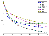
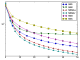
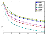
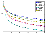
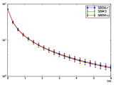
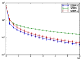
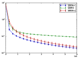
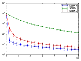
In this section, we examine the theoretical advantages of SBDA through several preliminary experiments. For all the algorithms compared, we estimate the parameters and tune the best stepsizes using separate validation data. We first investigate the performance of SBDA on nonsmooth deterministic problems by comparing its performance against other nonsmooth algorithms. We compare with the following algorithms: SM1 and SM2 are subgradient mirror decent methods with stepsizes $\gamma_{1}\propto\frac{1}{\sqrt{t}}$ and $\gamma_{2}\propto\frac{1}{\|g\left(x\right)\|}$ respectively. Finally, SGD is stochastic mirror descent and SDA a stochastic subgradient dual averaging method. We study the problem of robust linear regression ($\ell_{1}$ regression) with the objective $\phi\left(x\right)=\frac{1}{m}\sum_{i=1}^{m}\left|b_{i}-a_{i}^{T}x\right|$. The optimal solution $x^{*}$ and each $a_{i}$ are generated from $\mathcal{N}\left(0,I_{n\times n}\right)$. In addition, we define a scaling vector $s\in\mathbb{R}^{n}$ and $S$ a diagonal matrix s.t. $S_{ii}=s_{i}$. We let $b=\left(AS\right)x^{*}+\sigma$, where $A=\left[a_{2},a_{2},\ldots,a_{m}\right]^{T}\in\mathbb{R}^{m\times n}$, and the noise $\sigma\sim\mathcal{N}\left(0,\rho I\right)$ . We set $\rho=0.01$ and $m=n=5000$.

We plot the optimization objective with the number of passes of the dataset in Figure 1, for four different choices of $s$. In the first test case (leftmost subfigure), we let $s=\left[1,1,\ldots,1\right]^{T}$ so that columns of $A$ correspond to uniform scaling. We find that SBDA-u and SBDA-r have slightly better performance than the other algorithms while exhibiting very similar performance. In the next three cases, $s$ is generated from the distribution $p\left(x;a\right)=a\left(1-x\right)^{a-1}$, $0\leq x\leq 1$, $a>0$. We set $a=1,5,30$ respectively. Employing a large $a$ ensures that the bounds on the norms of block subgradients follow the power law. We observe that stochastic methods outperform the deterministic methods, and SBDA-based algorithms have comparable and often better performance than SGD algorithms. In particular, SBDA-r exhibits the best performance, which clearly shows the advantage of SBDA with the nonuniform sampling scheme.

Refer to caption
Refer to caption
Refer to caption
Refer to caption
Figure 1: Tests on $\ell_{1}$ regression.

Next, we examine the performance of SBDA for online learning and stochastic approximation. We conduct simulated experiments on the problem: $\phi\left(x\right)=\mathbf{E}_{a,b}\left[(b-\langle La,x\rangle)^{2}\right],$ where the aim is to fit linear regression under a linear transform $L$. The transform matrix $L\in M^{n\times n}$ is generated as follows: we first sample a matrix $\tilde{L}$ for which each entry $\tilde{L}_{i,j}\sim\mathcal{N}(0,1)$. $L$ is obtained from $\tilde{L}$ with $90\%$ of the rows being randomly rescaled by a factor $\rho$. To obtain the optimal solution $x^{*}$, we first generate a random vector from the distribution $\mathcal{N}(0,I_{n\times n})$ and then truncate each coordinate in $[-1,1]$. Simulated samples are generated according to $b=\langle La,x^{*}\rangle+\varepsilon$ where $\varepsilon\in\mathcal{N}(0,0.01I_{n\times n})$. We let $n=200$, and generate 3000 independent samples for training and 10000 independent samples for testing.

To compare the performances of these algorithms under various conditions, we tune the parameter $\rho$ in $[1,0.1,0.05,0.01]$. As can be seen from above, $\rho$ affects the estimation of block-wise parameters $\left\{M_{i}\right\}$. In Figure 2, we show the objective function for the average of 20 runs. The experimental results show the advantages of SBDA over SBMD. When $\rho=1$, SBDA-u, SBDA-r, and SBMD have the same theoretical convergence rate, and exhibit similar performance. However, as $\rho$ decreases, the “importance” of $90\%$ of the blocks is diminishing and we find SBDA-u and SBDA-r both outperform SBMD. Moreover, SBDA-r seems to perform the best, suggesting the advantage of our proposed stepsize and sampling schemes which are adaptive to the block structures. These observations lends empirical support to our theoretical analysis.

Refer to caption
Refer to caption
Refer to caption
Refer to caption
Figure 2: Tests on linear regression, Left to right: $\rho=1,0.1,0.05,0.01$.

Our next experiment considers online $\ell_{1}$ regularized linear regression (Lasso):

$$\min_{w\in\mathbb{R}^{n}}\frac{1}{2}\mathbf{E}_{\left(y,x\right)}\left[\left(y-w^{T}x\right)^{2}\right]+\lambda\|w\|_{1}$$ (41)

While linear regression has been well studied in the literature, recent work is interested in efficient regression algorithms under different adversarial circumstances [1, 9, 10]. Under the assumptions of limit budgets, the learner only partially observes the features for each incoming instance, but is allowed to choose the sampling distribution of the features. In addition, we explicitly enforce the $\ell_{1}$ penalty, expecting to learn a sparse solution that effectively reduces testing cost. To apply stochastic methods, we estimate the stochastic coordinate gradient of the least squares loss. For the sake of simplicity, we assume for each input sample instance $\left(y,x\right)$, two features $\left(i_{t},j_{t}\right)$ are revealed. When we sample one coordinate $j_{t}$ from some distribution $\left\{p_{j}\right\}$, then $\frac{1}{p_{j_{t}}}w^{(j_{t})}x^{(j_{t})}$ is an unbiased estimator of $w^{T}x$. Hence the defined value $G^{\left(i_{t}\right)}=\frac{1}{p_{j_{t}}}x^{\left(i_{t}\right)}x^{\left(j_{t}\right)}w^{\left(j_{t}\right)}-yx^{\left(i_{t}\right)}$ is an unbiased estimator of the $i_{t}$-th coordinate gradient.

We adapt both SBMD and SBDA-u to these problems and conduct the experiments on datasets covtype and mnist (digit “3 vs 5”). We also implement MD (composite mirror descent) and DA (regularized dual averaging method). For all the methods, the training uses the same total number of features. However, SBMD and SBDA-u obtain features sampled using a uniform distribution; both MD and DA have “unfair” access to observe full feature vectors and therefore have the advantages of lower variance. We plot in Figures 3a and 3b, the optimization error and sparsity patterns with respect to the penalty weights $\lambda$ on the two datasets. It can be seen that SBDA-u has comparable and often better optimization accuracy than SBMD. In addition, we also plot the sparsity patterns for different values of $\lambda$. It can be seen that SBDA-u is very effective in enhancing sparsity, more efficient than SBMD, MD, and comparable to DA which doesn’t have such budget constraints.

Refer to caption
Refer to caption
(a) Test on covtype dataset.
Refer to caption
Refer to caption
(b) Test on mnist dataset.
Figure 3: Tests on online lasso with limited budgets

6 Discussion

In this paper we introduced SBDA, a new family of block subgradient methods for nonsmooth and stochastic optimization, based on a novel extension of dual averaging methods. We specialized SBDA-u for regularized problems with nonsmooth or strongly convex regularizers, and SBDA-r for general nonsmooth problems. We proposed novel randomized stepsizes and optimal sampling schemes which are truly block adaptive, and thereby obtain a set of sharper bounds. Experiments demonstrate the advantage of SBDA methods compared with subgradient methods on nonsmooth deterministic and stochastic optimization. In the future, we will extend SBDA to an important class of regularized learning problems consisting of the finite sum of differentiable losses. On such problems, recent work [31, 32] shows efficient BCD convergence at linear rate. The works in [39, 35] propose randomized BCD methods that sample both primal and dual variables. However both methods apply conservative stepsizes which take the maximum of the block Lipschitz constant. It would be interesting to see whether our techniques of block-wise stepsizes and nonuniform sampling can be applied in this setting as well to obtain improved performance.

7 Appendix

Proof of Lemma 1

Proof.

The first part comes from [34]. Let $g\left(z\right)$ denote any subgradient of $f$ at $z$. Since $f\left(x\right)$ is strongly convex, we have $f\left(x\right)\geq f\left(z\right)+\langle U_{i}g^{\left(i\right)}\left(z\right),x-z\rangle+\frac{\lambda}{2}\|x-z\|_{\left(i\right)}^{2}$. By the definition of $z$ and optimality condition, we have $g^{\left(i\right)}\left(z\right)=-\nabla_{i}d\left(z\right)$. Thus

$$f\left(x\right)+\left\langle\nabla_{i}d\left(z\right),x-z\right\rangle\geq f\left(z\right)+\frac{\lambda}{2}\|x-z\|_{\left(i\right)}^{2}.$$

It remains to apply the definition $x=z+U_{i}y$ and $\mathcal{V}\left(z,x\right)=d\left(x\right)-d\left(z\right)-\left\langle\nabla d\left(z\right),x-z\right\rangle$. ∎

Proof of Lemma 2

Proof.

Let $h\left(y\right)=\max_{x\in X}\left\{\left\langle y,x\right\rangle-\Psi\left(x\right)\right\}$, since $\Psi\left(\cdot\right)$ is strongly convex and separable, $h\left(\cdot\right)$ is convex and differentiable and its $i$-th block gradient $\nabla_{i}h\left(\cdot\right)$ is $\frac{1}{\rho_{i}}$-smooth . Moreover, we have $\nabla h\left(0\right)=x_{0}$ by the definition of $x_{0}$. Thus

$$h\left(-U_{i}g^{\left(i\right)}\right)\leq h\left(0\right)+\left\langle x_{0},-U_{i}g^{\left(i\right)}\right\rangle+\frac{1}{2\rho_{i}}\|g\|_{\left(i\right),*}^{2}.$$

It remains to plug in the definition of $h\left(\cdot\right)$, $z$, $x_{0}$. ∎

Proof of Lemma 3

Conjecture.

By convexity of $f\left(\cdot\right)$, we have $f(z)\leq f(x)+\langle g(z),z-x\rangle$. In addition,

$\displaystyle\langle g(z),z-x\rangle$ $\displaystyle=$ $\displaystyle\langle g(x),z-x\rangle+\langle g(z)-g(x),z-x\rangle$
$\displaystyle=$ $\displaystyle\langle g^{(i)}(x),y\rangle_{(i)}+\langle g^{(i)}(z)-g^{(i)}(x),y\rangle_{(i)}$
$\displaystyle\leq$ $\displaystyle\langle g^{(i)}(x),y\rangle_{(i)}+\|g^{(i)}(z)-g^{(i)}(x)\|_{(i),*}\cdot\|y\|_{(i)}.$

The second equation follows from the relation between $x,y,z$ and the last one from the Cauchy-Schwarz inequality. Finally the conclusion directly follows from (5).

Proof of Lemma 5

Proof.

Let $A_{t}=\sum_{s=0}^{t}a_{t}$, $B_{t}=\sum_{s=1}^{t}b_{t}$. It is equivalent to show $A_{t}\leq B_{t}+\frac{A_{0}}{p}$. Then

$\displaystyle A_{t}$ $\displaystyle=pB_{t}+A_{0}+\left(1-p\right)A_{t-1}$
$\displaystyle=\left[p+\left(1-p\right)\right]\left[pB_{t-1}+A_{0}\right]+\left(1-p\right)^{2}A_{t-2}$
$\displaystyle=\left[p+\left(1-p\right)+\left(1-p\right)^{2}\right]\left[pB_{t-1}+A_{0}\right]+\left(1-p\right)^{3}A_{t-3}$
$\displaystyle=...$
$\displaystyle\leq$ $\displaystyle\left[pB_{t}+A_{0}\right]\left[\sum_{s=0}^{t}\left(1-p\right)^{s}\right].$

The last inequality follows from the assumption that $B_{t}\geq B_{s}$ where $0\leq s\leq t$ and $A_{0}=a_{0}$. It remains to apply the inequality $\sum_{s=0}^{t}\left(1-p\right)^{s}\leq\sum_{s=0}^{\infty}\left(1-p\right)^{s}=\frac{1}{p}$. ∎

Proof of Lemma 7

Proof.

If $r_{1},r_{2},r_{3}\sim\text{Bernoulli}\left(p\right)$, $c>0$, $0<p<1$,

$\displaystyle\mathbf{E}\left[\frac{1}{r_{1}x+r_{2}\left(a-x\right)+b}\right]$ $\displaystyle=$ $\displaystyle\frac{\left(1-p\right)^{2}}{b}+\frac{p\left(1-p\right)}{a-x+b}+\frac{p\left(1-p\right)}{x+b}+\frac{p^{2}}{a+b}$
$\displaystyle\leq$ $\displaystyle\frac{\left(1-p\right)^{2}}{b}+\frac{p\left(1-p\right)}{a+b}+\frac{p\left(1-p\right)}{b}+\frac{p^{2}}{a+b}$
$\displaystyle=$ $\displaystyle\frac{1-p}{b}+\frac{p}{a+b}$
$\displaystyle=$ $\displaystyle\mathbf{E}\left[\frac{1}{r_{3}a+b}\right].$

To see the first inequality, let $f\left(x\right)=\frac{A}{x+c}+\frac{B}{a-x+c}$, where $A,B>0$, it can be seen that $f\left(\cdot\right)$ is convex in $\left[0,a\right]$, then $\max_{x\in\left[0,a\right]}f\left(x\right)=\max\left\{f\left(0\right),f\left(a\right)\right\}$. ∎

Proof of Lemma 10

Proof.

Let $x^{*}$, $y^{*}$ be the optimal solution of $\min_{x,y}\mathcal{L}\left(x,y,a,b\right)$. We consider two subproblems. Firstly, $x^{*}=\arg\min_{x}\mathcal{L}\left(x,y^{*},a,b\right)$. Since $\frac{a_{i}}{x_{i}}+\frac{x_{i}}{b_{i}y_{i}^{*}}\geq 2\sqrt{\frac{a_{i}}{b_{i}y_{i}^{*}}}$, at optimality

$$\frac{a_{i}}{x_{i}^{*}}=\frac{x_{i}^{*}}{b_{i}y_{i}^{*}}.$$ (42)

On the other hand, $y^{*}$ is the minimizer of the problem $\min_{y}\mathcal{L}\left(x^{*},y,a,b\right)$. Applying the Cauchy-Schwarz inequality to $\mathcal{L}\left(x^{*},y,a,b\right)$, we obtain

$$\sum_{i=1}^{n}\frac{x_{i}^{*}}{b_{i}y_{i}}\cdot 1=\sum_{i=1}^{n}\frac{x_{i}^{*}}{b_{i}y_{i}}\sum_{1}^{n}y_{i}\geq\sum_{i}^{n}\sqrt{\frac{x_{i}^{*}}{b_{i}y_{i}}}\sqrt{y_{i}}=\sum_{i}^{n}\sqrt{x_{i}^{*}}.$$

At optimality, the equality holds for some scalar $C>0$,

$$\frac{x_{i}^{*}}{b_{i}y_{i}^{*}}=Cy_{i}^{*},\quad i=1,2,\ldots,n.$$ (43)

It remains to solve the equations (42) and (43) with the simplex constraint on $y$. ∎

References

  • [1] N. Cesa-Bianchi, S. Shalev-Shwartz, and O. Shamir. Efficient learning with partially observed attributes. The Journal of Machine Learning Research (JMLR), 12:2857–2878, 2011.
  • [2] X. Chen, Q. Lin, and J. Pena. Optimal regularized dual averaging methods for stochastic optimization. In Advances in Neural Information Processing Systems (NIPS) 25, 2012.
  • [3] C. D. Dang and G. Lan. Stochastic block mirror descent methods for nonsmooth and stochastic optimization. SIAM Journal on Optimization, 25(2):856–881, 2015.
  • [4] J. Duchi and Y. Singer. Efficient online and batch learning using forward backward splitting. Journal of Machine Learning Research (JMLR), 10:2899–2934, 2009.
  • [5] J. C. Duchi, S. Shalev-Shwartz, Y. Singer, and A. Tewari. Composite objective mirror descent. In The 23rd Conference on Learning Theory (COLT), 2010.
  • [6] S. Ghadimi and G. Lan. Optimal stochastic approximation algorithms for strongly convex stochastic composite optimization I: a generic algorithmic framework. SIAM Journal on Optimization, 22(4):1469–1492, 2012.
  • [7] L. A. Hageman and D. M. Young. Applied iterative methods. Courier Corporation, 2012.
  • [8] E. Hazan and S. Kale. Beyond the regret minimization barrier: optimal algorithms for stochastic strongly-convex optimization. The Journal of Machine Learning Research (JMLR), 15(1):2489–2512, 2014.
  • [9] E. Hazan and T. Koren. Linear regression with limited observation. In Proceedings of the 29th International Conference on Machine Learning (ICML), 2012.
  • [10] D. Kukliansky and O. Shamir. Attribute efficient linear regression with data-dependent sampling. arXiv preprint arXiv:1410.6382, 2014.
  • [11] S. Lacoste-Julien, M. Jaggi, M. Schmidt, and P. Pletscher. Block-coordinate Frank-Wolfe optimization for structural SVMs. In Proceedings of The 30th International Conference on Machine Learning (ICML), 2013.
  • [12] S. Lacoste-Julien, M. Schmidt, and F. Bach. A simpler approach to obtaining an ${O}(1/t)$ convergence rate for the projected stochastic subgradient method. arXiv preprint arXiv:1212.2002, 2012.
  • [13] G. Lan. An optimal method for stochastic composite optimization. Mathematical Programming, 133(1-2):365–397, 2012.
  • [14] G. Lan, Z. Lu, and R. D. Monteiro. Primal-dual first-order methods with $\{$ $\backslash$ mathcal $\{$O$\}$(1/$\backslash$ epsilon)$\}$ iteration-complexity for cone programming. Mathematical Programming, 126(1):1–29, 2011.
  • [15] J. Langford, L. Li, and T. Zhang. Sparse online learning via truncated gradient. Journal of Machine Learning Research (JMLR), 10:719–743, 2009.
  • [16] Y. T. Lee and A. Sidford. Efficient accelerated coordinate descent methods and faster algorithms for solving linear systems. In Proceedings of the 54th Annual IEEE Symposium on Foundations of Computer Science, pages 147–156, 2013.
  • [17] Z. Lu and L. Xiao. On the complexity analysis of randomized block-coordinate descent methods. Mathematical Programming, pages 1–28, 2014.
  • [18] Z. Q. Luo and P. Tseng. On the convergence of a matrix splitting algorithm for the symmetric monotone linear complementarity problem. SIAM Journal on Control and Optimization, 29(5):1037–1060, 1991.
  • [19] Z. Q. Luo and P. Tseng. On the convergence of the coordinate descent method for convex differentiable minimization. Journal of Optimization Theory and Applications, 72(1):7–35, Jan. 1992.
  • [20] A. Nedic and S. Lee. On stochastic subgradient mirror-descent algorithm with weighted averaging. SIAM Journal on Optimization, 24(1):84–107, 2014.
  • [21] A. Nemirovski, A. Juditsky, G. Lan, and A. Shapiro. Robust stochastic approximation approach to stochastic programming. SIAM Journal on Optimization, 19(4):1574–1609, Jan. 2009.
  • [22] Y. Nesterov. Primal-dual subgradient methods for convex problems. Mathematical Programming, 120(1):221–259, 2009.
  • [23] Y. Nesterov. Efficiency of coordinate descent methods on huge-scale optimization problems. SIAM Journal on Optimization, 22(2):341–362, 2012.
  • [24] Y. Nesterov. Subgradient methods for huge-scale optimization problems. Mathematical Programming, 146(1-2):275–297, 2014.
  • [25] Z. Qu and P. Richtárik. Coordinate descent with arbitrary sampling, I: Algorithms and complexity. arXiv preprint arXiv:1412.8060, 2014.
  • [26] A. Rakhlin, O. Shamir, and K. Sridharan. Making gradient descent optimal for strongly convex stochastic optimization. In Proceedings of the 29th International Conference on Machine Learning (ICML-12), pages 449–456, 2012.
  • [27] S. Reddi, A. Hefny, C. Downey, A. Dubey, and S. Sra. Large-scale randomized-coordinate descent methods with non-separable linear constraints. arXiv preprint arXiv:1409.2617, 2014.
  • [28] P. Richtárik and M. Takáč. Iteration complexity of randomized block-coordinate descent methods for minimizing a composite function. Mathematical Programming, 144(1-2):1–38, 2014.
  • [29] H. Robbins and S. Monro. A stochastic approximation method. The Annals of Mathematical Statistics, pages 400–407, 1951.
  • [30] S. Shalev-Shwartz and A. Tewari. Stochastic methods for $\ell_{1}$-regularized loss minimization. The Journal of Machine Learning Research (JMLR), 12:1865–1892, 2011.
  • [31] S. Shalev-Shwartz and T. Zhang. Stochastic dual coordinate ascent methods for regularized loss minimization. arXiv preprint arXiv:1209.1873, 2012.
  • [32] S. Shalev-Shwartz and T. Zhang. Accelerated proximal stochastic dual coordinate ascent for regularized loss minimization. arXiv preprint arXiv:1309.2375, 2013.
  • [33] Y. Singer and J. C. Duchi. Efficient learning using forward-backward splitting. In Advances in Neural Information Processing Systems (NIPS) 22, pages 495–503, 2009.
  • [34] P. Tseng. On accelerated proximal gradient methods for convex-concave optimization. submitted to SIAM Journal on Optimization, 2008.
  • [35] H. Wang and A. Banerjee. Randomized block coordinate descent for online and stochastic optimization. arXiv preprint arXiv:1407.0107, 2014.
  • [36] L. Xiao. Dual averaging methods for regularized stochastic learning and online optimization. The Journal of Machine Learning Research (JMLR), 11:2543–2596, 2010.
  • [37] Y. Xu and W. Yin. Block stochastic gradient iteration for convex and nonconvex optimization. arXiv preprint arXiv:1408.2597, 2014.
  • [38] P. Zhao and T. Zhang. Stochastic optimization with importance sampling. arXiv preprint arXiv:1401.2753, 2014.
  • [39] T. Zhao, M. Yu, Y. Wang, R. Arora, and H. Liu. Accelerated mini-batch randomized block coordinate descent method. In Advances in Neural Information Processing Systems (NIPS) 27, 2014.