Entanglement Entropy from Corner Transfer Matrix in Forrester Baxter non-unitary RSOS models

Abstract

Using a Corner Transfer Matrix approach, we compute the bipartite entanglement Rényi entropy in the off-critical perturbations of non-unitary conformal minimal models realised by lattice spin chains Hamiltonians related to the Forrester Baxter RSOS models [30] in regime III. This allows to show on a set of explicit examples that the Rényi entropies for non-unitary theories rescale near criticality as the logarithm of the correlation length with a coefficient proportional to the effective central charge. This complements a similar result, recently established for the size rescaling at the critical point [23], showing the expected agreement of the two behaviours. We also compute the first subleading unusual correction to the scaling behaviour, showing that it is expressible in terms of expansions of various fractional powers of the correlation length, related to the differences $\Delta-\Delta_{\min}$ between the conformal dimensions of fields in the theory and the minimal conformal dimension. Finally, a few observations on the limit leading to the off-critical logarithmic minimal models of Pearce and Seaton [49] are put forward.

PACS numbers: 03.65.Ud, 05.70.Jk, 05.50.+q, 02.30.Ik

Email: Davide.Bianchini.1@city.ac.uk, francesco.ravanini@bo.infn.it

Introduction

Entanglement is a very specific and intriguing feature of quantum systems [1]. It describes truly quantum correlations between parts of a system. Besides the questions of principal nature that it arises in the interpretation and behaviour of quantum mechanics [2, 3], it finds very interesting and promising applications in quantum information theory and quantum computing [4], in condensed matter physics [5, 6], as well as in the physics of black holes [7] and has even risen some interest in biological systems [8].

Many proposals have been formulated to quantify it (see for example [9] and references therein). In this paper we focus on bipartite systems, composed of a subsystem $A$ and its complement $\bar{A}$. In such case, the most convenient measure of entanglement is the Von Neumann Entropy restricted to $A$, the so-called Entanglement Entropy [4]. It is used as a measure of entanglement for pure quantum states. The behaviour of this quantity has been deeply studied in a wide range of systems from analytical, numerical and experimental points of view. For example, interesting experimental protocols in many body systems have been recently proposed [10, 11]. It has been evaluated in different dimensions and in different regimes, but it is in $1+1$ dimensions that it shows its most amazing mathematical properties. In particular, in the case of Integrable Models, it reflects many mathematical features that otherwise would be difficult to probe. For example, the study of Entanglement Entropy in critical one-dimensional quantum systems is one of the most powerful techniques for the identification of the central charge $c$ of the conformal field theory describing the low energy excitations of the model. This evaluation can be performed both analytically and numerically (e.g. DMRG [12]) and usually requires less information than the study of the scaling of the ground state energy for the identification of the universality class.

In the last decade there has been a particular focus on the evaluation of Entanglement Entropy in Integrable models, in particular in Conformal Field Theory (CFT) [13, 14], in their massive perturbations [15, 16] and in lattice spin chains [17, 18, 19, 20, 21, 22]. Recently also non unitary models have been taken into account, both in the critical [23] and in the massive [24] regimes.

At first sight, non unitary theories might be considered just as non physical mathematical curiosities, but there are many very interesting examples where they actually do play a physical role. For example, it is known that a strongly interacting 2D electron gas in a magnetic field produces edge modes described by CFT minimal models, in what is known as Fractional Quantum Hall Effect (FQHE). In some cases it has been shown that these edge modes are described by non unitary CFT [25]. In [26], for example, the minimal model $\mathcal{M}_{3,5}$ has been considered. The non-unitarity arises from the fact that in this particular case the bulk is gapless (while in the ordinary case it is gapped) and then the edge can dissipate into the bulk.

These excitations can be represented using generalised spin chains: the critical Fibonacci Chain (the “golden chain” [27], minimal model $\mathcal{M}_{4,5}$), which represents the FQHE with filling $\nu=\frac{12}{5}$ and its non-unitary generalisation to the Lee-Yang Model $\mathcal{M}_{2,5}$ [28] are among the most known chain representations. These critical chains all belong to the wide class of $\mathcal{U}_{q}(sl(2))$ invariant spin chains [29] in the universality class of conformal minimal models $\mathcal{M}_{m,m^{\prime}}$, unitary or not. They can be further generalised in order to include their massive $\Phi_{13}$ perturbations. The off-critical Hamiltonians of such chains have been recently obtained [30] and they are related to the RSOS models [31, 32], through the usual connection between the time evolution operators of 1D quantum spin chains and the row-to-row transfer matrix of 2D classical lattice models.

The Hamiltonians of these chains are generically of the pseudo-hermitian type, i.e. they are not hermitian but have real eignevalues. In recent years they attracted a lot of interest in the description of many physical phenomena, ranging from optical effects to non-equilibrium systems, etc… Similarly, in Quantum Field Theory it has been widely discussed [33] how the scattering matrices of apparently non-hermitian theories can be physically well defined. In particular, using the definitions of [33], non-unitary theories can be classified as real or non real; in both cases the inner product is indefinite, but in real theories eigenenergies are real and the eigenvalues of the S matrix are pure phases, while in non real models the energies are not real and the S matrix has eigenvalues which are not pure phases. Notice that if the S matrix is a pure phase, there is a conservation of probability through the scattering process; this conservation is a fundamental requirement for having a real, well-defined quantum physical theory.

Our goal in this paper is to compute the bipartite Entanglement Entropy of the ground state for spin chain hamiltonians of the type introduced in [30] on an infinite one dimesional lattice, taking as $A$ the negative semi-axis and as $\bar{A}$ the positive one. For non-Hermitian hamiltonians this may sound ambiguous, as non Hermitian operators share the same right and left eigenvalues but have different right and left eigenvectors. However, one can argue [23] using PT symmetry and chiral factorization of CFT that, at least at criticality, the left and right ground states do coincide, thus leading to a correct positive definition of the Entanglement Entropy for this state.

This bipartite Entanglement Entropy calculation can be achieved by considering the Corner Transfer Matrix (CTM) introduced by Rodney Baxter [34] in integrable statistical systems on a 2D square lattice. This tool, originally used for the evaluation of partition functions and one point functions of the 2D models, has been extended to the evaluation of the Entanglement Entropy of the corresponding 1D chains, following an approach developed in [17].

It is known that these chains, as well as their classical 2D counterparts, the class of RSOS_r,s models, show different regimes with different physical behaviour. In the unitary case $s=1$, Andrews, Baxter and Forrester (ABF) [31] classified four regimes. There are two second order phase transitions: one between regimes I and II and the other between regimes III and IV. The identification of universality classes at the transition points has been studied by Huse [35]. Approaching the III-IV transition the RSOS_r,1 models, for different $r$, are described by the universality class of unitary CFT minimal models $\mathcal{M}_{r-1,r}$. In the I-II phase transition, instead, the approach to criticality is governed by the universality class of $\mathbb{Z}_{L}$ parafermionic CFTs [36] with $L=r-2$.

In the non unitary cases $s\not=1$ explored in [32], the classification of regimes is more complicated. However, still there are regimes III and IV (or X if $r$ odd and $s=\frac{r-1}{2}$) with a phase transition between them identified [37, 38] with the universality class of non-unitary minimal models $\mathcal{M}_{r-s,r}$. The identification of the universality class of the regime I-II phase transition is still an open problem in the $s\not=1$ case. We shall not address this problem here and in the following we restrict our calculations to regime III.

In the case of unitary ABF RSOS models, Franchini and De Luca [39] have recently used the CTM technique to compute the Entanglement Entropy, checking that in the phase transition III-IV it correctly gives the results expected in the conformal unitary minimal models $\mathcal{M}_{r-1,r}$ while in the regime I-II phase transition, it gives those expected for the $\mathbb{Z}_{r-2}$ parafermionic CFTs.

In this paper we extend this Entanglement Entropy calculation to the regime III of $s\not=1$ RSOS models. The main goal of this investigation is to test on a concrete example of non unitary integrable theories where the calculations can be carried out exactly, the conjecture that the Entanglement Entropy scales logarithmically in the correlation length in a manner that parallels the scaling on a finite interval at criticality (for details of what we mean here see subsect. 2).

The paper is organised as follows:

• In section 1 we recall a few notions on minimal CFT models (unitary or not) and their characters, emphasising their relation with modular forms.

• Then in section 2 we introduce the basic concept and formulae of Rényi and Von Neumann Entanglement Entropies. We discuss in particular their behaviour for finite size of the subsystem at criticality and for infinte size but off-criticality. We consider in both cases the dominating logarithmic term, but also the form of the expected corrections.

• In section 3 we describe the Forrester-Baxter (FB) RSOS models whose continuum scaling limit is described by the perturbed minimal model $\mathcal{M}_{m,m^{\prime}}+t\Phi_{1,3}$ (where $t>0$ is a perturbing parameter and $\Phi_{1,3}$ the least relevant operator).

• We briefly summarise in section 4 the Corner Transfer Matrix construction and review its use as a tool for the evaluation of partition functions and Rényi Entropy. In particular, specialising to the RSOS models, we emphasise the connection between the blocks in the partition functions on multi-sheeted surfaces with the conformal characters of the corresponding CFT at criticality.

• Applying the CTM tool to the FB RSOS model, in section 5 we evaluate the Rényi Entropy for these theories. Our main results are the confirmation of the presence of the effective central charge in the leading scaling of the Entropy [23]. The difference from the unitary case where the usual central charge appears is due to the fact that the physical ground state and the conformal vacuum do not coincide in non unitary models.

• In section 6 we evaluate explicitly the most relevant corrections – nowadays traditionally called unusual corrections following [40] – to the dominating logarithmic behaviour. They exhibit power law decays with exponents given by a sort of effective dimensions, i.e. the difference between the conformal dimensions of some of the relevant fields of the CFT universality class and the lowest (negative) conformal dimension that always appears in non unitary CFTs.

• In section 7 we briefly comment on the evaluation of Rényi Entropy in off-critical Logarithmic Minimal Models, which can be seen as particular limit realisations of the FB RSOS model. The observed absence of the double log behaviour is related to the destruction of the Jordan block structures responsible of the logarithmic behaviour as soon as the log-CFT are perturbed off-criticality.

• Finally, in section 8 we trace our conclusions and perspectives for future work.

1 CFT minimal models and their characters

We recall here some basic facts about conformal minimal models that we need in the following. The minimal models $\mathcal{M}_{m,m^{\prime}}$ are conformal theories whose Hilbert space is built up of two chiral parts each one composed of a finite number of irreducible highest-weight representations (HWR) of Virasoro algebra at a given value of its central charge $c$. They are labelled by two coprime integers $m,m^{\prime}$ such that $2\leq m<m^{\prime}$ and have central charge

$$c=1-\frac{6(m-m^{\prime})^{2}}{mm^{\prime}}$$ (1.1)

The (left) conformal families $[\Phi_{a,a^{\prime}}]$ are labelled by two integers $a,a^{\prime}$ running on the domain $\mathcal{J}=\{(a,a^{\prime})\,:\,1\leq a\leq m-1\,,\,1\leq a^{\prime}\leq m^{\prime}-1\}$. The conformal dimensions of the primary states $|a,a^{\prime}\rangle$ of such families are given by

$$\Delta_{a,a^{\prime}}=\frac{(am^{\prime}-a^{\prime}m)^{2}-(m-m^{\prime})^{2}}{4mm^{\prime}}$$ (1.2)

The $\mathbb{Z}_{2}$ symmetry $\Delta_{a,a^{\prime}}=\Delta_{m-a,m^{\prime}-a^{\prime}}$ is present in the whole series of models.

The models are unitary for $m^{\prime}=m+1$, non unitary otherwise. In the non unitary case the state of lowest conformal dimension is not the conformal vacuum $|0\rangle\equiv|\Phi_{1,1}\rangle$ but a different state $|\mathrm{min}\rangle$ with negative conformal dimension (that can be proven always to exist and be unique)

$$\Delta_{\mathrm{min}}=\frac{1-(m-m^{\prime})^{2}}{4mm^{\prime}}$$ (1.3)

Correspondingly, an effective central charge can be defined

$$c_{\mathrm{eff}}=c-24\Delta_{\min}=1-\frac{6}{mm^{\prime}}$$ (1.4)

Notice that while the central charge $c$ can be negative in non unitary models, the effective one $c_{\mathrm{eff}}$ is always positive.

The characters of the Virasoro HWRs can be written as

$$\chi_{a,a^{\prime}}(q)=\frac{q^{\Delta_{a,a^{\prime}}-\frac{c}{24}}}{(q)_{\infty}}\sum_{k=-\infty}^{\infty}\left[q^{k(kmm^{\prime}+am^{\prime}\text{\textminus}a^{\prime}m)}-q^{(km+a)(km^{\prime}+a^{\prime})}\right]$$ (1.5)

where $q=e^{2\pi i\tau}$ and $(q)_{\infty}=\prod_{j=1}^{\infty}(1-q^{j})$. They form a unitary representation of the modular group [41] $PSL(2,\mathbb{Z})$ whose generators are

$$\hat{\mathcal{T}}\, : \,\tau\to\tau+1$$

$$\hat{\mathcal{S}}\, : \,\tau\to-\frac{1}{\tau}$$

$$\hat{\mathcal{T}}\chi_{a,a^{\prime}}(q) = \chi_{a,a^{\prime}}(qe^{2\pi i})=e^{2\pi i\left(\Delta_{a,a^{\prime}}-\frac{c}{24}\right)}\chi_{a,a^{\prime}}(q)$$

$$\hat{\mathcal{S}}\chi_{a,a^{\prime}}(q) = \chi_{a,a^{\prime}}\left(\tilde{q}\right)=\sum_{(b,b^{\prime})\in\mathcal{J}}\mathcal{S}_{a,a^{\prime}}^{b,b^{\prime}}\chi_{b,b^{\prime}}(q)$$ (1.6)

where $\tilde{q}=e^{-\frac{2\pi i}{\tau}}$. $\mathcal{S}$ is the modular matrix

$$\mathcal{S}_{a,a^{\prime}}^{b,b^{\prime}}=2\sqrt{\frac{2}{mm^{\prime}}}(-1)^{1+ab^{\prime}+a^{\prime}b}\sin\left(\pi\frac{m}{m^{\prime}}ab\right)\sin\left(\pi\frac{m^{\prime}}{m}a^{\prime}b^{\prime}\right)$$ (1.7)

Introducing the elliptic function

$$E(z,q)=\sum_{k\in\mathbb{Z}}(-1)^{k}q^{\frac{k(k-1)}{2}}z^{k}=\prod_{n=1}^{\infty}(1-q^{n-1}z)(1-q^{n}z^{-1})(1-q^{n})$$ (1.8)

they can equivalently be written as

$$\chi_{a,a^{\prime}}(q)=\frac{q^{\Delta_{a,a^{\prime}}-\frac{c}{24}}}{(q)_{\infty}}\left\{E\left(-q^{m^{\prime}a-a^{\prime}m+mm^{\prime}},q{}^{2mm^{\prime}}\right)-q^{aa^{\prime}}E\left(-q^{m^{\prime}a+a^{\prime}m+mm^{\prime}},q^{2mm^{\prime}}\right)\right\}$$ (1.9)

The function $E(z,q)$ is related to the first Jacobi theta function

$$\vartheta_{1}(u;p)=\sum_{n\in\mathbb{Z}}(-1)^{n-\frac{1}{2}}p^{\left(n+\frac{1}{2}\right)^{2}}e^{(2n+1)iu}=2p^{\frac{1}{4}}\sin u\prod_{n=1}^{\infty}(1-2p^{2n}\cos 2u+p^{4n})(1-p^{2n})$$ (1.10)

by the relation

$$E\left(e^{2iw},q\right)=iq^{-\frac{1}{8}}e^{iw}\vartheta_{1}(w;q^{\frac{1}{2}})$$ (1.11)

The first Jacobi theta function, under a modular $\hat{\mathcal{S}}$ tranformation, behaves as

$$\vartheta_{1}(z,e^{-\frac{i\pi}{\tau}})=-i\sqrt{i\tau}e^{\frac{i\tau z^{2}}{\pi}}\vartheta_{1}(\tau z;e^{i\pi\tau})$$ (1.12)

These formulae will be useful later in sect. 5 for the computation of the Rényi Entropy.

The minimal models can be perturbed off-criticality by picking up combinations of their relevant fields, resulting in super-renormalizable theories. In particular, the perturbation by the least relevant field $\Phi_{1,3}$ preserves the integrability of the model off-criticality. It is this integrable perturbation that represents the scaling limit of the RSOS models in the off-critical vicinity of the phase transition between regimes III and IV.

2 Rényi Entanglement Entropies

Consider a bipartite quantum system whose Hilbert space is $\mathcal{H}=\mathcal{H}_{A}\otimes\mathcal{H}_{\bar{A}}$. If the system is in a pure state $|\Psi\rangle$ (i.e. one with density matrix $\rho=|\Psi\rangle\langle\Psi|$), the entanglement between the two parts $A$ and its complement $\bar{A}$ can be described by the family of Rényi Entanglement Entropies $S_{n}$ ($n\in\mathbb{R}_{>0}$)

$$S_{A}^{(n)}=\frac{1}{1-n}\log\,\mbox{tr}_{A}\rho_{A}^{n}$$ (2.1)

where $\rho_{A}=\mbox{tr}_{\bar{A}}\rho$ is the reduced density matrix of the subsystem $A$. The Von Neumann Entanglement Entropy $S=\lim\limits_{n\rightarrow 1}S_{A}^{(n)}=-\mbox{tr}{}_{A}\left(\rho_{A}\log\rho_{A}\right)$ is a special case of the Rényi Entropies.

In [13, 14] it has been shown that the Rényi Entropy for a bipartite one-dimensional quantum system scales as

$$S_{A}^{(n)}\sim\frac{c}{6}\frac{n+1}{n}\log\frac{l}{\epsilon}$$ (2.2)

where $l$ is the size of the subsystem $A$, and $\epsilon$ is some ultraviolet cut-off. This scaling holds when the size of the whole system is much larger than the size $l$ of subsystem $A$ and when the correlation length $\xi$ is much larger than $l$. This condition on the correlation length is equivalent to assume that the system is approaching criticality with a universality class identified by a CFT with central charge $c$. In [40] the subleading contributions to this behaviour were estimated and look like

$$S_{A}^{(n)}\sim\frac{c}{6}\frac{n+1}{n}\log\frac{l}{\epsilon}+a^{(n)}+b^{(n)}l^{-2x/n}+b^{\prime(n)}l^{-2x}+...$$ (2.3)

The constants $a^{(n)}$, $b^{(n)}$ and $b^{\prime(n)}$ are non-universal, but the exponent $x$ is, and has to be identified with the scale dimension $x=\Delta+\bar{\Delta}$ of some operator $\Phi$ of the CFT universality class having the lowest conformal dimension among those concurring to the corrections. Higher order corrections are expected and they are due to other primary fields and to descendents. For $n>1$ the $l^{-2x}$ term is subleading with respect to the $l^{-2x/n}$ one. Viceversa for $n<1$. Taking into account both terms is necessary to ensure a smooth limit for $n\to 1$.

On the other hand, if the correlation length $\xi$ is finite and the size $l\rightarrow\infty$ we have [42] a similar expansion

$$S_{A}^{(n)}\sim\frac{c}{12}\frac{n+1}{n}\log\xi+A^{(n)}+B^{(n)}\xi^{-h/n}+B^{\prime(n)}\xi^{-h}+...$$ (2.4)

which represents the entanglement between two infinite parts of an infinite system. In this case the size $l$ of the subsystem $A$ has been replaced by the correlation length. This is due to the fact that the leading term of the Entropy is given by the smallest physical length which plays a role in the system. The factor of 2 difference in the leading terms and in the corrections is simply explained by the fact that the number of boundary points dividing $A$ from $\bar{A}$ is 2 in the first case and 1 in the second. The non-universal coefficients of the corrections $A^{(n)}$, $B^{(n)}$and $B^{\prime(n)}$ in general can be different from the $a^{(n)},b^{(n)},b^{\prime(n)}$ of eq.(2.3). Also, the universal exponent $h$ can differ from the $x$ above [21, 39].

Recently [23] this evaluation has been extended in order to take into account non unitary systems. The Hamiltonian operator $\hat{H}$ describing a CFT system of Hilbert space $\mathcal{H}$ put on a cylinder of circumference $R$ is given by

$$\hat{H}=\frac{2\pi}{R}\left(L_{0}+\bar{L}_{0}-\frac{c}{12}\right)$$ (2.5)

where $L_{n},\bar{L}_{n}$ are Virasoro algebra generators and $c$ is their central charge. In unitary CFT the conformal vacuum $|0\rangle$ (defined as the unique state such that $L_{n}|0\rangle=0$, $\forall n\geq-1$) is the physical ground state, i.e. $\forall|\psi\rangle\in\mathcal{H}:$ $\langle 0|\hat{H}|0\rangle\leq\langle\psi|\hat{H}|\psi\rangle$). Thus the ground state energy will scale as $E_{0}=-\frac{\pi c}{6R}$ [43, 44].

In non unitary CFT instead, there is at least one primary state $|\mathrm{min}\rangle$ with negative conformal weight $\Delta_{\mathrm{min}}$ ($\langle\mathrm{min}|L_{0}|\mathrm{min}\rangle=\Delta_{\mathrm{min}}<0$). Obviously, this state and not the conformal vacuum $|0\rangle$ has the lowest possible energy on the cylinder and is the true ground state of the theory. For this reason the ground state energy scales as $E_{\mathrm{min}}=-\frac{\pi c_{\mathrm{eff}}}{6R}$, with the so called effective central charge $c_{\mathrm{eff}}=c-24\Delta_{\mathrm{min}}\geq 0$ instead of the central charge $c$ [45]. The difference between the conformal vacuum and the physical ground state plays an important role in the definition and calculation of the Entanglement Entropy. For a detailed discussion, see [23]. As a result, in non-unitary CFT the Rényi Entropy scales as

$$S_{A}^{(n)}\sim\frac{c_{\mathrm{eff}}}{6}\frac{n+1}{n}\log\frac{l}{\epsilon}$$ (2.6)

Although this result seems natural, its proof in a generic non unitary CFT is far from trivial and can be acheived by a careful analysis of how to correctly define twist operators in such case through an orbifold approach [23].

In the case of infinite subsystem, one is tempted to replace $\frac{l}{\epsilon}$ by $\xi$, the correlation length, as in the unitary cases. In this paper our aim is to verify that this conjecture is correct in a concrete lattice realization of an off-critical non-unitary model. We use the RSOS non-unitary models of Forrester Baxter in regime III as lattice regularizations of the perturbed CFT $\mathcal{M}_{m,m^{\prime}}+t\Phi_{1,3}$ (where $t>0$ is a perturbing parameter).

In other words, we try in this paper to reproduce a formula of the type

$$S_{A}^{(n)}\sim\frac{c_{\mathrm{eff}}}{12}\frac{n+1}{n}\log\xi+A^{(n)}+B^{(n)}\xi^{-\frac{h}{n}}+B^{\prime(n)}\xi^{-h}$$ (2.7)

calculating it from the exact expression for the Rényi Entanglement Entropy obtainable by a Corner Transfer Matrix approach combined with the evaluation of the correlation length $\xi$ on the lattice. We expect that the exponent $h$ is affected by the non unitarity in a way similar to the change from $c$ to $c_{\mathrm{eff}}$ in the leading logarithmic term.

3 RSOS FB Models

The Restricted-Solid-On-Solid RSOS_r,s model [31, 32] is defined on a square lattice, for each pair of coprime positive integers $r,s$ such that $r>3$ and $1\leq s\leq r-1$. On each site $i\in\mathbb{Z}^{2}$ there is a variable, called local height, $\ell_{i}$ that takes values $\ell_{i}=1,2,\dots,r-1$. Local heights of two neighbouring sites $i$ and $j$ are restricted to differ by one $|\ell_{i}-\ell_{j}|=1$. Local heights can be thought as encoded on a $A_{r-1}$ Dynkin diagram. Each node represents a possible value that $\ell_{i}$ can take and it is linked to the possible values at neighbouring sites. This allows to generalise the model, following Pasquier [46], to other simply laced $A,D,E$ Dynkin diagrams. For the scope of the present paper, however, we focus on the $A$ case only. The RSOS models belong to the wide class of 2D classical lattice model of IRF (Interaction Round a Face) type. In IRF models, the interaction is on nearest neighbour, so that one can define local Boltzmann weights that depend on the four sites $i,j,k,l$ around a tile (see fig. 1)

Figure 1: Square tile

$$W\left(\begin{array}[]{cc}\ell_{l}&\ell_{k}\\ \ell_{i}&\ell_{j}\end{array}\right)=e^{-\beta\varepsilon_{ij}^{lk}}$$ (3.1)

where $\beta$ is the inverse temperature, $\varepsilon_{ij}^{lk}$ is the energy of the configuration of the four vertices.

For the RSOS models, the Boltzmann weights have been calculated from Yang-Baxter equation, that must be satisfied by any integrable lattice model, in [31, 32]. They depend on a spectral parameter $u$, measuring the anisotropy of the lattice, on the crossing parameter

$$\lambda=\frac{s}{r}\pi$$ (3.2)

ruling their behaviour when the lattice is rotated by $\frac{\pi}{2}$

$$W\left(\left.\begin{array}[]{cc}\ell_{l}&\ell_{k}\\ \ell_{i}&\ell_{j}\end{array}\right|u\right)=\sqrt{\frac{s(\ell_{i}\lambda)s(\ell_{k}\lambda)}{s(\ell_{j}\lambda)s(\ell_{l}\lambda)}}W\left(\left.\begin{array}[]{cc}\ell_{k}&\ell_{j}\\ \ell_{l}&\ell_{i}\end{array}\right|\lambda-u\right)$$ (3.3)

and on a temperature-like parameter $p$, ($-1<p<1$), such that $t=p^{2}$ is measuring the departure from criticality. The system is critical for $p=0$. The Boltzmann weights turn out to be expressible in terms of elliptic theta functions for which the parameter $p$ plays the rôle of the nome. Here and below $s(u)=\vartheta_{1}(u;p)$, the first Jacobi theta function (1.10). The non-zero Boltzmann weights can be put in the following form (in the so called symmetric gauge)

$$W\left(\left.\begin{array}[]{cc}\ell\pm 1&\ell\\ \ell&\ell\mp 1\end{array}\right|u\right) =\frac{s(\lambda-u)}{s(\lambda)}$$ (3.6)

$$W\left(\left.\begin{array}[]{cc}\ell&\ell\pm 1\\ \ell\mp 1&\ell\end{array}\right|u\right) =\frac{\sqrt{s((\ell\mp 1)\lambda)s((\ell\pm 1)\lambda)}}{s(\ell\lambda)}\frac{s(u)}{s(\lambda)}$$ (3.9)

$$W\left(\left.\begin{array}[]{cc}\ell&\ell\pm 1\\ \ell\pm 1&\ell\end{array}\right|u\right) =\frac{s(\ell\lambda\pm u)}{s(\ell\lambda)}$$ (3.12)

The periodicity and modular properties of the Boltzmann weights determine the fundamental ranges of the parameters. The classification of possible regimes of the models is quite complicated [32] but in this paper we concentrate on regime III ($0<p<1$ and $0<u<\lambda$) only, leaving the others for future investigation.

For $s=1$ the model, often denoted simply RSOS_r, has been investigated by Andrews, Baxter and Forrester in [31]. The Rényi Entanglement Entropy for the cooresponding spin chains has been computed in [39], where it is shown that in the regime III approaching the critical point $p=0$ it scales like (2.4) with the central charge of unitary minimal models $\mathcal{M}_{r-1,r}$. In the regime II transition, instead, it scales as the parafermions $\mathbb{Z}_{r-2}$.

Here we are interested in the generalizations of these results for other values of $s$. The spin chains Hamiltonians corresponding to the RSOS_r,s models have been recently written in [30]. As the notation for them is quite complicated and not relevant for the following, we do not write them here and invite the interested reader to refer to the paper [30] for an exhaustive presentation.

4 The Corner Transfer Matrix approach

For spin chains on an infinite 1D lattice, we consider the Renyi Entanglement Entropy between two semi-infinite halves, the negative one conventionally called $A$ while the positive is $\bar{A}$. For chains related to a 2D classical lattice model of IRF (Interaction Round a Face) type, an efficient method to compute the reduced density matrix $\rho_{A}$, as proposed in [17], is to make use of the Corner Transfer Matrix approach [34]. The FB RSOS models are of this kind, therefore we adopt this approach here.

Consider the 2D “diamond shaped” lattice of fig.2

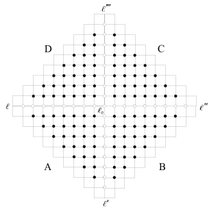
Figure 2: The 4 corner transfer matrix operators

and divide it in four quadrants. The central site is denoted by 0. In the lower-left quadrant $\boldsymbol{\mathsf{A}}$ introduce an operator (see fig. 2)

$$\mathbf{A}_{\boldsymbol{\ell},\boldsymbol{\ell}^{\prime}}^{(N)}(u)={\displaystyle\delta_{\ell_{0},\ell_{0}^{\prime}}\sum_{\ell_{i}|i=\bullet\in\boldsymbol{\mathsf{A}}}\prod_{\square\in\boldsymbol{\mathsf{A}}}}W\left(\left.\begin{array}[]{cc}\ell_{l}&\ell_{k}\\ \ell_{i}&\ell_{j}\end{array}\right|u\right)$$ (4.1)

where $\boldsymbol{\ell}=(\ell_{0},\ell_{1},\ell_{2},...,\ell_{N})$ and $\boldsymbol{\ell}^{\prime}=(\ell_{0}^{\prime},\ell_{1}^{\prime},\ell_{2}^{\prime},...,\ell_{N}^{\prime})$ are vectors collecting all the variables along the two inner boundaries, i.e. on the sites denoted by $\circ$ in fig. 2. The sum is performed over all possible values of $\ell_{i}$ on internal sites (signed by a black dot $\bullet$ in fig. 2). The variables at the outer boundary sites are assigned fixed values determining a boundary condition uniquely. The product is over all tiles $\square$ of the quadrant. Notice the $\ell_{0}=\ell_{0}^{\prime}$ obvious constraint on the central site 0.

Analogously, define in the other quadrants the operators $\mathbf{B}_{\boldsymbol{\ell}^{\prime},\boldsymbol{\ell}^{\prime\prime}}^{(N)}$, $\mathbf{C}_{\boldsymbol{\ell}^{\prime\prime},\boldsymbol{\ell}^{\prime\prime\prime}}^{(N)}$ and $\mathbf{D}_{\boldsymbol{\ell}^{\prime\prime\prime},\boldsymbol{\ell}}^{(N)}$. Organizing the product of $W$’s to be performed diagonally (thus the diamond shape of the lattice), a corner transfer matrix like $\mathbf{A}_{\boldsymbol{\ell},\boldsymbol{\ell}^{\prime}}^{(N)}$ may be expressed in terms of smaller corner transfer matrices $\mathbf{A}_{\boldsymbol{\ell},\boldsymbol{\ell}^{\prime}}^{(N-1)}$ and $\mathbf{A}_{\boldsymbol{\ell},\boldsymbol{\ell}^{\prime}}^{(N-2)}$ (defined for reduced quadrants). This recursion relation allows, in principle, the iterative calculation of the corner transfer matrix for any lattice quadrant of finite size.

The partition function can be expressed in terms of the four CTM operators as

$$Z^{(N)}=\mbox{tr}(\mathbf{A}^{(N)}\mathbf{B}^{(N)}\mathbf{C}^{(N)}\mathbf{D}^{(N)})$$ (4.2)

There are other interesting quantities that can be computed form the CTM method, like e.g. the height probabilities. Here we are interested in the calculation of the reduced density matrix $\rho_{A}$ relative to a dominion $A$ coinciding with the negative axis of the horiziontal direction of the infinite lattice that results taking the thermodynamic limit $N\to\infty$ of the present construction. Following [17], the unnormalised reduced density matrix on the subsystem $A$ can be written as

$$\varrho_{A,\boldsymbol{\ell}\boldsymbol{\ell}^{\prime}}=(\mathbf{ABCD})_{\boldsymbol{\ell}\boldsymbol{\ell}^{\prime}}$$ (4.3)

where $\mathbf{A}=\lim_{N\to\infty}\mathbf{A}^{(N)}$ and analogously for B, C, D. Obviously $\mbox{tr}_{A}\varrho_{A}=\mathcal{Z}_{1}$ is the partition function in the thermodynamic limit

$$\mathcal{Z}_{1}=\lim_{N\to\infty}Z^{(N)}$$ (4.4)

To normalise, one has to divide by the partition function

$$\rho_{A,\boldsymbol{\ell}\boldsymbol{\ell}^{\prime}}=\frac{(\mathbf{ABCD})_{\boldsymbol{\ell}\boldsymbol{\ell}^{\prime}}}{\mathcal{Z}_{1}}$$ (4.5)

For the Rényi Entanglement Entropy we need to compute $\mbox{tr}_{A}\rho_{A}^{n}$. Defining the higher genus partition functions $\mbox{tr}_{A}\varrho_{A}^{n}=\mathcal{Z}_{n}$ one sees that

$$\mbox{tr}_{A}\rho_{A}^{n}=\frac{\mathcal{Z}_{n}}{\mathcal{Z}_{1}^{n}}$$ (4.6)

and the expression for the Rényi Entropy is

$$S_{A}^{(n)}=\frac{1}{1-n}\log\frac{\mathcal{Z}_{n}}{\mathcal{Z}_{1}^{n}}$$ (4.7)

As shown by Baxter [34], the Yang-Baxter equation that has to be satisfied by the Boltzamnn weights of any integrable model, implies that the four CTM operators, for $N\to\infty$, commute each other for different values of their parameters and their eigenvalues, up to a common factor, accommodate into a diagonal matrix of the general form

$$\varrho_{A,\boldsymbol{\ell}\boldsymbol{\ell}^{\prime}}^{\mathrm{diag}}=R(\ell_{0})T(\boldsymbol{\ell})\delta_{\boldsymbol{\ell},\boldsymbol{\ell}^{\prime}}$$ (4.8)

The diagonalisation can be performed along the lines illustrated in [34]. In particular, for FB RSOS models it has been performed in the original paper [32]. It is simplified if one introduces new variables $x$, $y$ that in regime III are defined as

$$y=e^{\frac{4\pi^{2}}{\log p}}\qquad,\qquad x=e^{\frac{4\pi^{2}}{\log p}\frac{s}{r}}=y^{\frac{s}{r}}$$ (4.9)

Define

$$\Phi(\boldsymbol{\ell})=\sum_{k=1}^{N}k\gamma(\ell_{k},\ell_{k+1},\ell_{k+2})$$ (4.10)

where

$$\gamma(\ell,\ell\pm 1,\ell)=\mp\left\lfloor\frac{\ell s}{r}\right\rfloor\qquad,\qquad\gamma(\ell\pm 1,\ell,\ell\mp 1)=\frac{1}{2}$$ (4.11)

In regime III we have

$$\Phi(\boldsymbol{\ell})=\sum_{k=1}^{N}\left\{k\frac{|\ell_{k}-\ell_{k+2}|}{4}+(\ell_{k}-\ell_{k+1})\left\lfloor\frac{\ell_{k}s}{r}\right\rfloor\right\}$$ (4.12)

The second term of the summand is absent in the $s=1$ case simply because $\left\lfloor\ell_{k}/r\right\rfloor$ is always 0. Consider now a system with size $2N+3$. The unormalised reduced density matrix in regime III, as computed in [32], is given by

$$\varrho_{A,\boldsymbol{\ell}\boldsymbol{\ell}^{\prime}}^{(N)}=\left(\mathbf{ABCD}\right)_{\boldsymbol{\ell}\boldsymbol{\ell}^{\prime}}^{(N)}=E\left(x^{\ell_{0}},y\right)x^{2\Phi(\boldsymbol{\ell})}\delta_{\boldsymbol{\ell}\boldsymbol{\ell}^{\prime}}$$ (4.13)

where $\ell_{0}$ is the central height and $\boldsymbol{\ell}=(\ell_{0},\dots,\ell_{N+1})$ is a vector of all local heights from the central to the boundary $\ell_{N+1}$. Here $E(\cdot,\cdot)$ is the modular form defined in (1.8).

5 Rényi Entropy in FB RSOS models

As disccussed in section 2, to compute the Rényi Entropy we need to consider not only $\varrho_{A}$ but also its $n$-th powers $\varrho_{A}^{n}$.

Let us set the boundary condition to $\ell_{N}=b$ and $\ell_{N+1}=c=b\pm 1$. The $n$-th power of the reduced density matrix is given by

$$(\varrho_{A}^{(N)})_{\boldsymbol{\ell}\boldsymbol{\ell}^{\prime}}^{n}=E\left(x^{\ell_{0}},y\right)^{n}x^{2n\Phi(\boldsymbol{\ell})}\delta_{\boldsymbol{\ell}\boldsymbol{\ell}^{\prime}}$$ (5.1)

The trace can be performed summing over all allowed configurations $\boldsymbol{\ell}$

$$Z_{n}^{(N)} = \sum_{\boldsymbol{\ell}}E\left(x^{\ell_{0}},y\right)^{n}x^{2n\Phi(\boldsymbol{\ell})}$$ (5.2)

$$\equiv \sideset{}{{}^{*}}{\sum}_{{a=1}}^{{r-1}}E\left(x^{a},y\right)^{n}D_{N}\left(a,b,c;x^{2n}\right)$$

where $D_{N}(a,b,c;q)=\sum\limits_{\ell_{1}\cdots\ell_{N-1}}q^{\Phi(\boldsymbol{\ell})}$ with $\ell_{0}=a$, $\ell_{N}=b$ and $\ell_{N+1}=c$. The $\sum^{*}$ symbol means that the sum is restricted to even or odd only values of $a$ accordingly to the parity of the boundary conditions. In particular notice the the central height $a$ and the boundary height $b$ have to be compatible with the requirement $|\ell_{i}-\ell_{i+1}|=1$.

The limit $N\rightarrow\infty$ can be performed, keeping track of the boundary condition $\ell_{N}\lessgtr\ell_{N+1}$:

$$\lim_{N\rightarrow\infty}q^{-\frac{kN}{2}}D_{N}(a,b,b+1;q)=\frac{1}{(q)_{\infty}}q^{\frac{b(b-1)}{4}-\frac{(k-1)b}{2}}F(a,b-k;q)$$ (5.3)

with $k=\lfloor\frac{s(b+1)}{r}\rfloor=\lfloor\frac{s\ell_{N+1}}{r}\rfloor$ if $\ell_{N}<\ell_{N+1}$ or

$$\lim_{N\rightarrow\infty}q^{\frac{kN}{2}}D_{N}(a,b+1,b;q)=\frac{1}{(q)_{\infty}}q^{\frac{b(b+1)}{4}-\frac{k(b+1)}{2}}F(a,b-k;q)$$ (5.4)

with $k=\lfloor\frac{sb}{r}\rfloor=\lfloor\frac{s\ell_{N+1}}{r}\rfloor$ if $\ell_{N}>\ell_{N+1}$.

The function $F$ is defined as

$$F(a,d;q) = q^{\frac{a(a-1)}{4}-\frac{ad}{2}}\left[E\left(-q^{rd+(r-a)(r-s)},q^{2r(r-s)}\right)-q^{ad}E\left(-q^{rd+(r-a)(r+s)},q^{2r(r-s)}\right)\right]$$ (5.5)

$$= q^{\frac{a(a-1)}{4}-\frac{ad}{2}}\frac{(q)_{\infty}}{q^{-\frac{c}{24}+\Delta_{da}}}\chi_{da}(q)$$

where the Virasoro characters $\chi_{da}(q)$ (see eq.(1.9)) are taken here for $m=r-s$ and $m^{\prime}=r$. Thus

$$\lim_{N\rightarrow\infty}q^{\mp\frac{kN}{2}}D_{N}(a;q)_{b,d=b-k}=q^{f_{\mp}(b,d)}q^{\frac{a(a-1)}{4}-\frac{ad}{2}+\frac{c}{24}-\Delta_{da}}\chi_{da}(q)$$ (5.6)

where

$$f_{+}(b,d) = \frac{b(b-1)}{4}-\frac{b(k-1)}{2}$$

$$f_{-}(b,d) = \frac{b(b+1)}{4}-\frac{k(b+1)}{2}$$ (5.7)

do not depend on $a$.

Since the physical (normalised) density operator is given by

$$\rho_{A}\equiv\frac{\varrho_{A}}{\mbox{Tr}_{A}\varrho_{A}}=\frac{\mathbf{ABCD}}{\mbox{Tr}(\mathbf{ABCD})}$$ (5.8)

the quantity in which we are interested is

$$\mbox{tr}_{A}{\rho_{A}}^{n}=\frac{\mathcal{Z}_{n}}{\mathcal{Z}_{1}^{n}}=\frac{\hat{\mathcal{Z}}_{n}}{\hat{\mathcal{Z}}_{1}^{n}}$$ (5.9)

where

$$\hat{\mathcal{Z}}_{n}={\displaystyle\sideset{}{{}^{*}}{\sum}_{{a=1}}^{{r-1}}}E\left(x^{a},y\right)^{n}x^{2n\left(\frac{a(a-1)}{4}-\frac{ad}{2}-\Delta_{da}\right)}\chi_{da}\left(x^{2n}\right)$$ (5.10)

since the factor $\left(f_{\mp}+\frac{c}{24}\right)^{n}$ appears in both the numerator and the denominator and cancels out.

Notice that the critical point is reached for $p\rightarrow 0$, or $x\rightarrow 1$. In order to catch the critical behaviour we transform (5.10) into a new expression which is more suitable for expansion near $p=0$. First of all we can use the relations (1.11) and (1.12) for the function $E$

$$\mathcal{W}_{n}=\sideset{}{{}^{*}}{\sum}_{{a=1}}^{{r-1}}\vartheta_{1}\left(\frac{\pi as}{r},\sqrt{p}\right)^{n}\chi_{da}\left(x^{2n}\right)$$ (5.11)

where, again, $\mathcal{W}_{n}$ is proportional to $\hat{\mathcal{Z}_{n}}$ and a common factor with $\hat{\mathcal{Z}}_{1}^{n}$ has been dropped so that

$$\mbox{tr}_{A}{\rho_{A}}^{n}=\frac{\mathcal{Z}_{n}}{\mathcal{Z}_{1}^{n}}=\frac{\hat{\mathcal{Z}}_{n}}{\hat{\mathcal{Z}}_{1}^{n}}=\frac{\mathcal{W}_{n}}{\mathcal{W}_{1}^{n}}$$ (5.12)

Furthermore we can perform a modular $\hat{\mathcal{S}}$ transformation (1.6) on the conformal character

$$\chi_{a,a^{\prime}}\left(\tilde{q}\right)=\sum_{(b,b^{\prime})\in\mathcal{J}}\mathcal{S}_{a,a^{\prime}}^{b,b^{\prime}}\chi_{b,b^{\prime}}(q)$$ (5.13)

Since $x^{2}=e^{\frac{8\pi^{2}}{\log p}\frac{s}{r}}=e^{2\pi i\left(-i\frac{4\pi}{\log p}\frac{s}{r}\right)}$, its modular $\hat{\mathcal{S}}$-transform is $\omega\equiv\widetilde{\left(x^{2}\right)}=e^{\frac{\log p}{2}\frac{r}{s}}=p^{\frac{r}{2s}}$ (recall that, in regime III, $p>0$). Similarly, $\widetilde{(x^{2n})}=(p^{\frac{r}{2s}})^{\frac{1}{n}}=\omega^{1/n}$. We have

$${\mathcal{W}}_{n}=\sideset{}{{}^{*}}{\sum}_{{a=1}}^{{r-1}}\sum_{d^{\prime}a^{\prime}}\vartheta_{1}\left(\frac{\pi as}{r},\sqrt{p}\right)^{n}\mathcal{S}_{da}^{d^{\prime}a^{\prime}}\chi_{d^{\prime}a^{\prime}}\left(\omega^{\frac{1}{n}}\right)$$ (5.14)

which is suitable for a $p\rightarrow 0$ expansion.

Denoting $\mathfrak{h}=(d^{\prime},a^{\prime})\in\mathcal{J}$ as an index which spans the Kac table we have

$$\mathcal{W}_{n} = \sum_{\mathfrak{h}\in\mathcal{J}}\chi_{\mathfrak{h}}\left(\omega^{\frac{1}{n}}\right)f_{\mathfrak{h}}\left(n,p\right)$$ (5.15)

$$= \chi_{\mathrm{min}}\left(\omega^{\frac{1}{n}}\right)f_{\mathrm{min}}\left(n,p\right)\left(1+\sum_{\mathfrak{h}\neq\mathrm{min}}\frac{\chi_{\mathfrak{h}}\left(\omega^{\frac{1}{n}}\right)}{\chi_{\mathrm{min}}\left(\omega^{\frac{1}{n}}\right)}\frac{f_{\mathfrak{h}}\left(n,p\right)}{f_{\mathrm{min}}\left(n,p\right)}\right)$$

where

$$f_{\mathfrak{h}}\left(n,p\right)=\sideset{}{{}^{*}}{\sum}_{{a=1}}^{{r-1}}\vartheta_{1}\left(\frac{\pi as}{r},\sqrt{p}\right)^{n}\mathcal{S}_{da}^{d^{\prime}a^{\prime}}$$ (5.16)

and $\mathfrak{h}=\mathrm{min}$ refers to the primary field with the lowest conformal dimension $\Delta_{\mathrm{min}}$.

Taking the logarithm, we have

$$\log\frac{\mathcal{W}_{n}}{{\mathcal{W}_{1}}^{n}} = \log\frac{\chi_{\mathrm{min}}\left(\omega^{\frac{1}{n}}\right)}{\chi_{\mathrm{min}}\left(\omega\right)^{n}}+\log\frac{f_{\mathrm{min}}\left(n,p\right)}{f_{\mathrm{min}}\left(1,p\right)^{n}}$$ (5.17)

$$+ \log\left(1+\sum_{\mathfrak{h}\neq\mathrm{min}}\frac{\chi_{\mathfrak{h}}\left(\omega^{\frac{1}{n}}\right)}{\chi_{\mathrm{min}}\left(\omega^{\frac{1}{n}}\right)}\frac{f_{\mathfrak{h}}\left(n,p\right)}{f_{\mathrm{min}}\left(n,p\right)}\right)$$

$$- n\log\left(1+\sum_{\mathfrak{h}\neq\mathrm{min}}\frac{\chi_{\mathfrak{h}}\left(\omega\right)}{\chi_{\mathrm{min}}\left(\omega\right)}\frac{f_{\mathfrak{h}}\left(1,p\right)}{f_{\mathrm{min}}\left(1,p\right)}\right)$$

Expanding $\chi_{\mathrm{min}}$ and $f_{\mathrm{min}}$ of the first two terms of the equation above near $p,\omega=0$ we obtain the leading scaling and the constant coefficient for the Rényi Entropy

$$S_{A}^{(n)} = -\frac{c_{\mathrm{eff}}}{24}\frac{n+1}{n}\log\omega+\tilde{A}^{(n)}$$ (5.18)

$$+ \frac{1}{1-n}\log\left(1+\sum_{\mathfrak{h}\neq\mathrm{min}}\frac{\chi_{\mathfrak{h}}\left(\omega^{\frac{1}{n}}\right)}{\chi_{\mathrm{min}}\left(\omega^{\frac{1}{n}}\right)}\frac{f_{\mathfrak{h}}\left(n,p\right)}{f_{\mathrm{min}}\left(n,p\right)}\right)$$

$$- \frac{n}{1-n}\log\left(1+\sum_{\mathfrak{h}\neq\mathrm{min}}\frac{\chi_{\mathfrak{h}}\left(\omega\right)}{\chi_{\mathrm{min}}\left(\omega\right)}\frac{f_{\mathfrak{h}}\left(1,p\right)}{f_{\mathrm{min}}\left(1,p\right)}\right)$$ (5.19)

The constant $\tilde{A}^{(n)}$ is given by

$$\tilde{A}^{(n)}=\frac{1}{1-n}\log\frac{\sideset{}{{}^{*}}{\sum}\limits_{{a=1}}^{{r-1}}\mathcal{S}_{da}^{\mathrm{min}}\sin^{n}\frac{\pi as}{r}}{\left(\sideset{}{{}^{*}}{\sum}\limits_{{a=1}}^{{r-1}}\mathcal{S}_{da}^{\mathrm{min}}\sin\frac{\pi as}{r}\right)^{n}}$$ (5.20)

which is well defined in the $n\rightarrow 1$ limit.

6 “Unusual” corrections

The next step is the evaluation of power law corrections to the logarithmic scaling of the Rényi Entropy. First, notice that $\chi_{\mathfrak{h}}\ll\chi_{\mathrm{min}}$ for $\omega\rightarrow 0$. In this regime the argument of the logarithms in the second and third line of (5.18) is close to $1$ and then it can be Taylor expanded. Taking into account only the most relevant contribution and assuming, to fix ideas, that $n>1$, we have

$$S_{A}^{(n)}=-\frac{c_{\mathrm{eff}}}{24}\frac{n+1}{n}\log\omega+\tilde{A}^{(n)}+\sum_{\mathfrak{h}\neq\mathrm{min}}\tilde{B}_{\mathfrak{h}}^{(n)}\omega^{\frac{\Delta_{\mathfrak{h}}-\Delta_{\mathrm{min}}}{n}}+\cdots$$ (6.1)

with

$$\tilde{B}_{\mathfrak{h}}^{(n)}=\frac{1}{1-n}\frac{\sum\limits_{a}\sin^{n}\frac{\pi as}{r}\mathcal{S}_{da}^{\mathfrak{h}}}{\sum\limits_{a}\sin^{n}\frac{\pi as}{r}\mathcal{S}_{da}^{\mathrm{min}}}$$ (6.2)

and the most relevant contribution is given by the second smallest conformal dimension among those appearing in the expansion of 5.18, denoted $\Delta_{1}$ in the following. Taking into account only this correction we have

$$S_{A}^{(n)}=-\frac{c_{\mathrm{eff}}}{24}\frac{n+1}{n}\log\omega+\tilde{A}^{(n)}+\tilde{B}_{1}^{(n)}\omega^{\frac{\Delta_{1}-\Delta_{\mathrm{min}}}{n}}+\cdots$$ (6.3)

In the case $n<1$ one can proceed similarly, but now the first correction will be

$$S_{A}^{(n)}=-\frac{c_{\mathrm{eff}}}{24}\frac{n+1}{n}\log\omega+\tilde{A}^{(n)}+\tilde{B}_{1}^{\prime(n)}\omega^{\Delta_{1}-\Delta_{\mathrm{min}}}+\cdots$$ (6.4)

with

$$\tilde{B}_{\mathfrak{h}}^{\prime(n)}=\frac{n}{1-n}\frac{\sum\limits_{a}\sin\frac{\pi as}{r}\mathcal{S}_{da}^{\mathfrak{h}}}{\sum\limits_{a}\sin\frac{\pi as}{r}\mathcal{S}_{da}^{\mathrm{min}}}=n\tilde{B}_{\mathfrak{h}}^{(1)}$$ (6.5)

In order to interpret these results from a physical point of view, i.e. to have an expression for the entropy in terms of the correlation length (or in term of the mass), we need a relation between the parameter $\omega=p^{\frac{r}{2s}}$ and the correlation length $\xi$. In other words, we need to know the critical exponent $\nu$ in regime III:

$$m\;\;\;=\;\;\;\xi^{-1}\sim p^{\nu}$$ (6.6)

Using perturbative CFT it is possible to evaluate the critical exponent $\nu$. In the continuum limit, the model is described by the perturbed CFT:

$$S=S_{\mathrm{CFT}}+t\int d^{2}x\;\Phi_{1,3}(x)$$ (6.7)

where $|t|=p^{2}$ measures the departure from criticality. A simple dimensional analysis of this action tells us that $\nu=\frac{1}{2(1-\Delta_{1,3})}=\frac{r}{4s}$ for the minimal model $\mathcal{M}_{r-s,r}$ at the transition between regime III and IV.

This value for the critical exponent $\nu$ can also be extracted extending previous results [47] to the Forrester Baxter models. Taking into account the necessary modifications, the calculation can be carried out along the same lines of [47] to get

$$e^{-\frac{1}{\xi}}=k^{\prime}(p^{\nu})$$ (6.8)

where $k^{\prime}(q)$ is the conjugate elliptic modulus for the elliptic nome $q$

$$k^{\prime}(q)=\prod_{\ell=1}^{\infty}\left(\frac{1-q^{2\ell-1}}{1+q^{2\ell-1}}\right)^{4}$$ (6.9)

Expanding (6.8) around $p=0$ we get

$$\xi^{-1}=8p^{\nu}+\frac{32}{3}p^{3\nu}+\frac{48}{5}p^{5\nu}+\frac{64}{7}p^{7\nu}+O(p^{9\nu})$$ (6.10)

in perfect agreement with the perturbative CFT prediction.

Using (4.9) and (6.10) we have $\omega=(8\xi)^{-2}+\cdots$ which gives

$$S_{A}^{(n)}=\frac{c_{\mathrm{eff}}}{12}\frac{n+1}{n}\log\xi+A^{(n)}+B_{1}^{(n)}\xi^{-\frac{2}{n}(\Delta_{1}-\Delta_{\mathrm{min}})}+nB_{1}^{(1)}\xi^{-2(\Delta_{1}-\Delta_{\min})}+...$$ (6.11)

where constants $A^{(n)}$ and $B_{1}^{(n)}$ are just trivial rescaling of $\tilde{A}^{(n)}$ and $\tilde{B}_{1}^{(n)}$:

$$A^{(n)} = \tilde{A}^{(n)}+\frac{c_{\mathrm{eff}}}{4}\frac{n+1}{n}\log 2$$ (6.12)

$$B_{1}^{(n)} = 8^{-\frac{2}{n}(\Delta_{1}-\Delta_{\mathrm{min}})}\tilde{B}_{1}^{(n)}$$ (6.13)

From the equation (6.12), it is immediately possible to read the correction to the logarithmic scaling. For unitary theories the correction is expected to scale as $\xi^{-\frac{2\Delta}{n}}$ where $\Delta$ is the conformal dimension of the field related to the correction [39]. In the non unitary case this term is affected by the fact that the ground state is no more the conformal vacuum $|0\rangle$ but another state $|\mathrm{min}\rangle=\Phi_{\mathrm{min}}(0,0)|0\rangle$. The formula $\Delta_{1}-\Delta_{\mathrm{min}}$ shows that the presence of a non trivial ground state modifies the scaling of the correction. It is known [23] that this feature affects also the logarithmic scaling of the entropy in non-unitary models, where the central charge $c$ is replaced by the effective one $c_{\mathrm{eff}}$. Similarly, it is not surprising that the conformal dimensions are replaced by some sort of “effective” dimensions $\Delta-\Delta_{\min}$. Notice that the unitary case can be immediately recovered in (6.12) by setting $\Delta_{\mathrm{min}}=0$.

7 A comment on off-critical Logarithmic Minimal Models

An interesting feature of Forrester Baxter RSOS models is that, for a particular choice of parameters $r$ and $s$, they provide a lattice realisation of Logarithmic Minimal models [48] and their off-critical thermal perturbations [49]. In particular it has been shown that in the limit $r,s\to\infty$, keeping the ratio $r/s$ fixed to some rational number $R/S$, the underlying model becomes the so called logarithmic minimal model $\mathcal{LM}_{R-S,R}$ and its off-critical thermal perturbation $\mathcal{LM}_{R-S,R}+t\Phi_{1,3}$ .

Taking such a limit for the entropy, the result is not affected from the functional point of view: it maintains the same structure and the effective central charge

$$c_{\mathrm{eff}}=\lim_{r,s\to\infty}\left(1-\frac{6}{r(r-s)}\right)$$ (7.1)

is identically 1 for any choice of the ratio $R/S$

$$S_{A}^{(n)}=\frac{1}{12}\frac{n+1}{n}\log\xi+\bar{A}^{(n)}+\bar{B}_{1}^{(n)}\xi^{-\frac{2}{n}(\Delta_{1}-\Delta_{\mathrm{min}})}+n\bar{B}_{1}^{(1)}\xi^{-2(\Delta_{1}-\Delta_{\mathrm{min}})}+\cdots$$ (7.2)

Here $\bar{B}_{1}^{(n)}={\displaystyle\lim_{r,s\to\infty}}B_{1}^{(n)}$. When taking the limit $r,s\to\infty$ the $\mathcal{S}$ modular matrix becomes ill defined because the prefactor $\sqrt{\frac{2}{r(r-s)}}=\frac{1}{r}\sqrt{\frac{2}{1-\frac{s}{r}}}$ tends to zero in this limit. While this feature does not affect the limit of the coefficent $B_{1}^{(n)}$ (6.2) – as $\mathcal{S}$ appears with the same power both at the numerator and at the denominator – it implies some extra attention for the limit of the constant $A^{(n)}$ (5.20). For this reason, we need to modify the definition of the Rényi Entropy for Logarithmic models multiplying the partition function by $r$ in a sort of renormalisation procedure

$$\bar{A}^{(n)}=\lim_{r,s\to\infty}\left(A^{(n)}-\log\frac{1}{r}\right)$$ (7.3)

This multiplication can be seen in the same spirit of defyning generalised order parameters in [49], while a better understanding of this renormalistion of the Entropy is still missing and goes far beyond the aim of this work. In any case, it only affects the numerical value of the non-universal constant $\bar{A}^{(n)}$ and not the functional shape of the $\xi$ dependence of the entropy.

This $\xi$ dependence result (7.2) disagrees with the general prediction for the Rényi Entropy $l$ dependence in logarithmic CFT [23], where a double logarithmic (log log) term is expected. The difference is due to the fact that the logarithmic feature of the system is related to the presence of non diagonalisable Jordan blocks in the Hamiltonian. It has been noticed in [49] that such non diagonalisability feature disappears as soon as the system is perturbed thermally out of the critical point. Thus the so called off-critical logarithmic minimal models are not really logarithmic and thus we should not expect double log term in the computation of the entropy. In the case of logarithmic minimal models, then, we expect that, while the dependence in the subsystem size $l$ at criticality rescales with a double logarithmic term, this is absent in the rescaling off-criticality in $\xi$ while approaching the logarithmic critical point. The two behaviours in this case are different, while in the usual minimal models (unitary or not) they show a similar (single log rescaling) pattern.

8 Conclusions and outlook

We have computed the Entanglement Rényi Entropy for Forrester-Baxter RSOS models in the regime III, a set of lattice systems whose continuum limit is described by non-unitary Minimal Conformal Models perturbed by their $\Phi_{1,3}$ operator. Our evaluation focused on the scaling with the correlation length $\xi$ of the Entropy for a infinite, bipartite, quantum system. The computation of Entanglement Entropy in non unitary models has been recently addressed in [23] and [24] where a logarithmic scaling with the size $l$ of the subsystem has been found. In particular it has been shown in [23] that the coefficient of the logarithm is given by the effective central charge $c_{\mathrm{eff}}$. For unitary theories the computation of the Entropy for a finite critical system ($l<\infty,\;m^{-1}=\xi=\infty$) can be easily translated [14] in the infinite subsystem with a small but non zero mass gap ($l=\infty,\;m^{-1}=\xi<\infty$) using arguments similar to the Zamolodchikov c-theorem. In the non unitary case such a translation cannot be performed a priori, since some assumptions about the positivity of certain correlation functions are no more valid in the non unitary case. For this reason, the scaling we have found, where the proper length $l$ is replaced by the correlation length $\xi$ gives a strong hint about the renormalisation flux properties in the non unitary case. A proof of a sort of $c_{\mathrm{eff}}$-theorem in the non unitary case goes far beyond the aim of this paper. Nevertheless, our result supports evidence, in a non trivial set of non unitary models, that the $\xi$ scaling follows the same logarithmic law of the $l$ scaling, exactly like in the unitary models.

We have also studied the power law corrections to the logarithmic scale of the Entropy. The interesting part is not in the coefficients of the expansion, that are non universal, but in the exponent of the power of $\xi$. In the unitary case the expansion organises into many series expansions in terms of powers of $\xi^{\Delta_{\mathfrak{h}}}$ or $\xi^{\Delta_{\mathfrak{h}}/n}$, with $\mathfrak{h}$ labelling the various conformal primary fields. In the non unitary case we find that the series expansions are in terms of $\xi^{\Delta_{\mathfrak{h}}-\Delta_{\min}}$ or $\xi^{(\Delta_{\mathfrak{h}}-\Delta_{\min})/n}$. In other words, also the conformal dimensions here take an “effective” value shifted by $\Delta_{\min}$, exactly like the central charge is replaced by $c_{\mathrm{eff}}$.

We have also briefly considered the limiting case of the off-critical Logarithmic Minimal Models. Even if a double logarithmic term has been expected from the literature [23], where the $l$ rescaling has been considered, we did not find here such a term: the scaling in $\xi$ behaves exactly as in the non-logarithmic case. This discrepancy is due to the fact that the perturbation outside the critical point destroys the Jordan blocks responsible for the creation of the logarithmic features, as already pointed out in [49].

It their seminal work on the FB RSOS model [32], Forrester and Baxter classified many regimes, while we have restricted our analysis to regime III only. While it is known [37, 38] that the regime III is a lattice realisation of the perturbed Minimal Models $\mathcal{M}_{r-s,r}+\Phi_{1,3}$, the physical interpretation of the other regimes has still to be explored. In the unitary ABF RSOS model [31], the number of regimes is smaller (just four, compared to ten in the FB case) and two kind of universality classes have been identified. The critical line between the Regime III and IV can be described by the Unitary Minimal Models $\mathcal{M}_{r-1,r}$, while a unitary parafermionic CFT $\mathbb{Z}_{r-2}$ underlies the critical line between regimes I and II. It would be very interesting to try to understand if some critical line of the FB RSOS model can be classified using, maybe, the non unitary parafermionc CFT introduced in [50] or if they obey instead some other classification scheme. The evaluation of Entanglement Entropy has been demonstrated to be a powerful tool for the identification of universality classes and it could be a valid help also in the study of the unknown regimes of the FB RSOS model.

Of course, further generalizations of these results to the lattice realisations of higher coset conformal filed theories perturbed by their $\Phi_{1,1,3}$ opertors, or even for models based on cosets of higher algebras, like $W_{n}$-algebra based series, including Pasquier like generalizations and their dilute versions, etc… can all be the subject of future investigation. As non unitary coset models as critical points of fusions of FB RSOS models are under construction right in these days [51], the exploration of Rényi Entanglement Entropies for this set of models is viable.

The bipartite Entanglement Entropy can give a lot of useful information, but a more complete understanding of entanglement needs also the knowledge of the dependence on the size of the system, as well as its behaviour in finite intervals. We know how to deal with these problems in CFT [14] and, with a form factor expansion, also in off-critical integrable quantum field theories [15]. However, in integrable spin chains, a useable procedure to compute entanglement entropies on a finite interval is still lacking in general. This would be a serious progress in our understanding of entanglement in one-dimensional systems.

Also, the interest in entanglement measurements with more than two subsystems introduces new quantites to be evaluated, like negativity [52, 53]. To find a way to compute these quantites in a consistent lattice integrable approach is a challenge for future research.

Acknowledgments

We are endebted to O. A. Castro-Alvaredo and B. Doyon for very useful discussions. In particular, we thank the fruitful and deep exchange of ideas with P. A. Pearce, as well as his continuous and encouraging interest in this work. We acknowledge E. Ercolessi for the advice and the deep discussions during the elaboration of the M.Sc. thesis of one of us (D.B.), where many of the results presented here were in nuce obtained. F.R. thanks INFN, and in particular its grant GAST, for partial financial support. D.B. thanks City University London for his Doctoral Scholarship and the University of Bologna for the warm hospitality when part of this work has been done.

References

- [1] E. Schrödinger, Discussion of probability relations between separated systems, Proc. Cambridge Phil. Soc. 31 (1935) 555
- [2] A. Einstein, B. Podolsky and N. Rosen, Can quantum-mechanical description of physical reality be considered complete?, Phys. Rev. 47 (1935) 777
- [3] J. S. Bell, On the Einstein-Podolsky-Rosen paradox, Physics 1 (1964) 195
- [4] C. H. Bennet, H. J. Bernstein, S. Popescu and B. Schumacher, Concentrating partial entanglement by local operations, Phys. Rev. A53 (1996) 2046
- [5] L. Amico, R. Fazio, A. Osterloh and V. Vedral, Entanglement in many-body systems, Rev. Mod. Phys. 80 (2008) 517
- [6] J. I. Latorre and A. Riera, A short review on entanglement in quantum spin systems, J. Phys. A42 (2009) 504002
- [7] S. N. Solodukhin, Entanglement Entropy of Black Holes, Living Rev. Relativity, 14 (2011) 8 and references therein
- [8] M. Sarovar, A. Ishizaki, G. R. Fleming and K. B. Whaley, Quantum entanglement in photosynthetic light-harvesting complexes, Nature Physics 6 (2010) 462–467
- [9] M. B. Plenio and S. Virmani, An introduction to entanglement measures, Quantum Inf. Comput. 7 (2007) 1.
- [10] D. Abanin and E. Demler, Measuring entanglement entropy of a generic many-body system with a quantum switch, Phys. Rev. Lett. 109 (2012) 020504
- [11] J. L. Cardy, Measuring entanglement using quantum quenches, Phys. Rev. Lett. 106 (2011) 150404
- [12] S. R. White, Density matrix formulation for quantum renormalization groups, Phys. Rev. Lett. 69 (1992) 2863
- [13] C. Holzhey, F. Larsen, F. Wilczek, Geometric and Renormalized Entropy in Conformal Field Theory, Nucl.Phys. B424 (1994) 443-467
- [14] P. Calabrese and J. L. Cardy, Entanglement entropy and quantum field theory, J. Stat. Mech. 0406 (2004) P06002
- [15] J. L. Cardy, O. Castro-Alvaredo and B. Doyon, Form factors of branch-point twist fields in quantum integrable models and entanglement entropy, J. Stat. Phys. 130 (2008) 129–168
- [16] B. Doyon, Bi-partite entanglement entropy in massive two-dimensional quantum field theory, Phys. Rev. Lett. 102 (2009) 031602
- [17] L. Kaulke, I. Peschel and M. Legeza, Density matrix spectra for integrable models, Ann. der Physik 8(2) (1999) 153–164
- [18] F. Franchini, A. Its and V. Korepin, Renyi Entropy of the XY Spin Chain J.Phys. A41 (2008) 025302
- [19] E. Ercolessi, S. Evangelisti and F. Ravanini, Exact entanglement entropy of the XYZ model and its sine- Gordon limit, Phys. Lett. A374 (2010) 2101-2105
- [20] E. Ercolessi, S. Evangelisti, F. Franchini and F. Ravanini, Essential singularity in the Renyi entanglement entropy of the one-dimensional XYZ spin-1/2 chain, Phys. Rev. B83 (2011) 012402
- [21] E. Ercolessi, S. Evangelisti, F. Franchini and F. Ravanini, Correlation Length and Unusual Corrections to the Entanglement Entropy, Phys. Rev. B85 (2012) 115428
- [22] E. Ercolessi, S. Evangelisti, F. Franchini and F. Ravanini, Modular invariance in the gapped XYZ spin-1/2 chain, Phys. Rev. B88 (2013) 104418
- [23] D. Bianchini, O. A. Castro-Alvaredo, B. Doyon, E. Levi and F. Ravanini, Entanglement Entropy of Non Unitary Conformal Field Theory, J. Phys. A: Math. Theor. 48 (2015) 04FT01
- [24] D. Bianchini, O. A, Castro-Alvaredo and B. Doyon, Entanglement Entropy of Non-Unitary Integrable Quantum Field Theory, Nucl.Phys. B896 (2015) 835-880
- [25] B. Estienne, N. Regnault, and B.A. Bernevig, Correlation Lengths and Topological Entanglement Entropies of Unitary and Nonunitary Fractional Quantum Hall Wave Functions, Phys. Rev. Lett. 114 (2015) 186801
- [26] S. H. Simon, E. H. Rezayi, N. R. Cooper and I. Berdnikov, Construction of a paired wave function for spinless electrons at filling fraction , Phys. Rev. B75 (2007) 075317
- [27] A. Feiguin, S. Trebst, A. W. W. Ludwig, M. Troyer, Al. Kitaev, Z. Wang, and M. H. Freedman, Interacting Anyons in Topological Quantum Liquids: The Golden Chain, Phys. Rev. Lett. 98 (2007) 160409
- [28] E. Ardonne, J. Gukelberger, A.W.W. Ludwig, S. Trebst and M. Troyer, Microscopic models of interacting Yang–Lee anyons, New J. Phys. 13 045006 (2011)
- [29] V. Pasquier and H. Saleur, Common structures between finite systems and conformal field theories through quantum groups, Nucl. Phys. B330 (1990) 523–556
- [30] D. Bianchini, E. Ercolessi, P. A. Pearce and F. Ravanini, RSOS quantum chains associated with off-critical minimal models and parafermions, J. Stat. Mech. 1503 (2015) P03010
- [31] G. Andrews, R. J. Baxter and P. Forrester, Eight vertex SOS model and generalized Rogers-Ramanujan type identities, J. Stat. Phys. 35 (1984) 193
- [32] P. J. Forrester and R. J. Baxter, Further exact solutions of the eight-vertex SOS model and generalizations of the Rogers-Ramanujan identities, J. Stat. Phys. 38 (1985) 435
- [33] G. Takács and G.M.T. Watts, RSOS revisited, Nucl. Phys. B 642 (2002) 456-482
- [34] R. J. Baxter, Exactly solved models in Statistical Mechanics, Academic Press (1982)
- [35] D. Huse, Exact exponents for infinitely many new multicritical points, Phys. Rev. B30 (1984) 3908–3915
- [36] V. A. Fateev and A. B. Zamolodchikov, Parafermionic Currents in the Two-Dimensional Conformal Quantum Field Theory and Selfdual Critical Points in Invariant Statistical Systems, Sov. Phys. JETP 62 (1985) 215-225
- [37] Riggs H, Solvable lattice models with minimal and nonunitary critical behaviour in two dimensions, Nucl. Phys. B326 (1989) 673
- [38] Nakanishi T, Non-unitary minimal models and RSOS models, Nucl. Phys. B334 (1990) 745
- [39] A. De Luca and F. Franchini, Approaching the restricted solid-on-solid critical points through entanglement: One model for many universalities, Phys. Rev. B 87 (2013) 045118
- [40] J. Cardy and P. Calabrese, Unusual Corrections to Scaling in Entanglement Entropy, J. Stat. Mech.: Theory Exp. 1004 (2010) P04023.
- [41] P. Di Francesco, P. Mathieu and D. Sénéchal, Conformal Field Theory, Springer (1997)
- [42] P. Calabrese, J. L. Cardy and I. Peschel, Corrections to scaling for block entanglement in massive spin-chains, J. Stat. Mech. 1009 (2010) P09003
- [43] I. Affleck, Universal term in the free energy at a critical point and the conformal anomaly, Phys. Rev. Lett. 56 (1986) 746–748
- [44] H. W. J. Blöte, J. L. Cardy and M. P. Nightingale, Conformal invariance, the central charge, and universal finite-size amplitudes at criticality, Phys. Rev. Lett. 56 (1986) 742–745
- [45] C. Itzykson, H. Saleur and J.-B. Zuber, Conformal invariance of nonunitary 2d-models, Europhys. Lett. 2 (1986) 91
- [46] V. Pasquier, Two-dimensional critical systems labelled by Dynkin diagrams, Nucl. Phys. B285 [FS19] (1987) 162–172
- [47] D. L. O’Brien and P. A. Pearce, Surface free energies, interfacial tensions and correlation lengths of the ABF models, J. Phys. A: Math. Gen. 30 (1997) 2353
- [48] P. A. Pearce, J. Rasmussen and J.-B. Zuber, Logarithmic minimal models, J. Stat. Mech. 0611 (2006) P11017
- [49] P. A. Pearce and K. Seaton, Off-critical logarithmic minimal models, J. Stat. Mech. 1209 (2012) P09014
- [50] C. Ahn, S. Chung and S. H. Tye, New parafermion SU(2) coset and N=2 superconformal field theories, Nucl. Phys. B 365 (1991) 191-240
- [51] E. Tartaglia and P. A. Pearce, Fused RSOS models as higher-level nonunitary minimal cosets, in preparation (2015)
- [52] P. Calabrese, J. L. Cardy and E. Tonni, Entanglement negativity in quantum field theory, Phys. Rev. Lett. 109 (2012) 130502
- [53] P. Calabrese, J. L. Cardy and E. Tonni, Entanglement negativity in extended systems: A field theoretical approach, J. Stat. Mech. 1302 (2013) P02008