Large non-factorizable contributions in $B\to a_{0}a_{0}$ decays

Abstract

We investigate three tree-dominated $B\to a_{0}a_{0}$ decays for the first time in the perturbative QCD(pQCD) approach at leading order in the standard model, with $a_{0}$ standing for the light scalar $a_{0}(980)$ state, which is assumed as a meson based on the model of conventional two-quark$(q\bar{q})$ structure. All the topologies of the Feynman diagrams such as the non-factorizable spectator ones and the annihilation ones are calculated in the pQCD approach. It is of great interest to find that, contrary to the known $B\to\pi\pi$ decays, the $B\to a_{0}a_{0}$ decays are governed by the large non-factorizable contributions, which give rise to the large $B\to a_{0}a_{0}$ decay rates in the order of $10^{-6}\sim 10^{-5}$, although the $a_{0}$ meson has an extremely small vector decay constant $f_{a_{0}}$. Also observed are large direct CP-violating asymmetries around $15\%$ and $30\%$ for the $B^{0}\to a_{0}^{0}a_{0}^{0}$ and $a_{0}^{+}a_{0}^{-}$ modes. These sizable predictions could be easily examined at the running Large Hadron Collider and the near future Super-B/Belle-II experiments. The future precision measurements combined with these pQCD predictions might be helpful to explore the complicated QCD dynamics and the inner structure of the light scalar $a_{0}$, as well as to complementarily constrain the unitary angle $\alpha$.

I Introduction

As we know, the nature of the light scalar states such as $a_{0}(980)$ is not yet well understood at both theoretical and experimental aspects. Also the identification and the classification of these light scalars remain as a long-standing puzzle(for latest review, see, e.g. Agashe:2014kda ) to be resolved. However, it is fortunate for the people that the light scalars as products in the heavy flavor meson decays have been detected, for example, $D\to SP,SV$, $B\to SP,SV$, even $B\to SS$ modes Agashe:2014kda ; Amhis:2014hma with $S,P,$ and $V$ being the light scalar, pseudoscalar, and vector mesons, respectively, which will provide unique places and play very important roles on investigating the physical properties of light scalars. It is generally believed that the ongoing Large Hadron Collider(LHC) experiments can provide rich data on the $B$, $B_{s}$, and $B_{c}$ meson decaying into light scalars. And more promisingly, the forthcoming Super-B/Belle-II factory scheduled in 2018 with a high luminosity ${\ \lower-1.2pt\vbox{\hbox{\hbox to0.0pt{$>$\hss}\lower 6.0pt\vbox{\hbox{$\sim$} }}}\ }10^{36}{\rm cm}^{-2}{\rm s}^{-1}$ Bona:2007qt ; Gershon:2006mt will produce much more events about the relevant decays. The studies on the above mentioned decays can also provide more constraints complementarily on the parameters in the standard model(SM), hint the exotic new physics beyond the SM, etc.

In this work, we will investigate the CP-averaged branching ratios and the CP-violating asymmetries of the $B\to a_{0}(980)a_{0}(980)$ decays by employing the perturbative QCD(pQCD) approach Keum:2000ph ; Lu:2000em ; Li:2003yj with the low energy effective Hamiltonian Buchalla:1995vs in the SM. It should be noted that the $a_{0}(980)$ state here will be assumed as a meson in the model of conventional two-quark$(q\bar{q})$ structure. Moreover, hereafter, the $a_{0}(980)$ will be abbreviated as $a_{0}$ for the sake of simplicity throughout the paper. To our knowledge, heretofore, no other $B\to SS$ processes have been studied explicitly in the factorization approaches based on the QCD dynamics, apart from the $B_{u,d,s}\to K_{0}^{*}(1430)\bar{K}_{0}^{*}(1430)$ decays Liu:2013lka by two of our authors (X. Liu and Z.J. Xiao). Because the scalar meson has either tiny or vanishing vector decay constant Cheng:2005nb ; Cheng:2009xz , the contributions arising from the factorizable emission diagrams in the $B\to SS$ decays are usually highly suppressed, which is dramatically different from the known $B\to PP,PV,VV$ decays. In other words, for example, in contrast to the extensively investigated $B\to\pi\pi$ decays, the large measured $B\to a_{0}a_{0}$ decay rates may indicate large non-factorizable spectator scattering and/or annihilation contributions, which would hint some useful information on the $B\to\pi\pi$ decays, the presently known puzzle to be resolved, because they embrace the same components at the quark level. In the heavy $B$ meson decays, the above mentioned large contributions from non-factorizable spectator and annihilation diagrams are often considered as the small and/or negligible higher order or higher power corrections in the naive factorization approach Bauer:1986bm . Therefore, the channels involving an emitted scalar state in the heavy flavor meson decays are suggested to test the breaking effects of the factorization assumption, e.g. Diehl:2001xe . Though the QCD improved factorization approach Beneke:1999br ; Du:2000ff going beyond the naive factorization, the end-point singularities make it less predictive because the non-factorizable spectator scattering contributions and the annihilation ones have to be parametrized with the tunable parameters, which are always determined by the experimental measurements. As one of the popular factorization approaches based on the QCD dynamics, the pQCD approach involves no end-point singularities by retaining the parton transverse momentum $k_{T}$. Based on $k_{T}$ factorization theorem, the double logarithms arising from the overlap of soft and collinear divergences generated in the radiative corrections are resummed into an important Sudakov factor to suppress the long-distance contribution Li:1996gi . Armed with this pQCD approach, all the transition form factors, the non-factorizable spectator diagrams, and the annihilation diagrams are perturbatively calculable, besides the factorizable spectator diagrams. Note that, as far as the annihilation contributions are concerned, soft-collinear effective theory Bauer:2004tj and pQCD approach have an extremely different effect on the perturbative calculations Arnesen:2006vb ; Chay:2007ep . However, the predictions on the pure annihilation decays based on the pQCD approach can accommodate the experimental data well, for example, see Refs. Lu:2002iv ; Li:2004ep ; Ali:2007ff ; Xiao:2011tx . We will therefore put the controversies aside and adopt the pQCD approach in our analyses.

The paper is organized as follows. Section II is devoted to the analytic expressions for the decay amplitudes of $B\to a_{0}a_{0}$ modes in the pQCD approach. The numerical results and phenomenological analyses on the CP-averaged branching ratios and the CP-violating asymmetries of the considered decays are given in Sec. III. We summarize and conclude in Sec. IV.

II Perturbative calculations

For the considered $B\to a_{0}a_{0}$ decays, the related weak effective Hamiltonian $H_{{\rm eff}}$ Buchalla:1995vs can be written as

$$H_{\rm eff}\, = \,{G_{F}\over\sqrt{2}}\biggl{\{}V^{*}_{ub}V_{ud}[C_{1}(\mu)O_{1}^{u}(\mu)+C_{2}(\mu)O_{2}^{u}(\mu)]-V^{*}_{tb}V_{td}[\sum_{i=3}^{10}C_{i}(\mu)O_{i}(\mu)]\biggr{\}}+{\rm H.c.}\;,$$ (1)

with the Fermi constant $G_{F}=1.16639\times 10^{-5}{\rm GeV}^{-2}$, the Cabibbo-Kobayashi-Maskawa(CKM) matrix elements $V$, and the Wilson coefficients $C_{i}(\mu)$ at the renormalization scale $\mu$. The local four-quark operators $O_{i}(i=1,\cdots,10)$ are written as

1. (1) current-current(tree) operators

   $${\begin{array}[]{ll}\displaystyle O_{1}^{u}\,=\,(\bar{d}_{\alpha}u_{\beta})_{V-A}(\bar{u}_{\beta}b_{\alpha})_{V-A}\;,&\displaystyle O_{2}^{u}\,=\,(\bar{d}_{\alpha}u_{\alpha})_{V-A}(\bar{u}_{\beta}b_{\beta})_{V-A}\;;\end{array}}$$ (3)

2. (2) QCD penguin operators

   $${\begin{array}[]{ll}\displaystyle O_{3}\,=\,(\bar{d}_{\alpha}b_{\alpha})_{V-A}\sum_{q^{\prime}}(\bar{q}^{\prime}_{\beta}q^{\prime}_{\beta})_{V-A}\;,&\displaystyle O_{4}\,=\,(\bar{d}_{\alpha}b_{\beta})_{V-A}\sum_{q^{\prime}}(\bar{q}^{\prime}_{\beta}q^{\prime}_{\alpha})_{V-A}\;,\\ \displaystyle O_{5}\,=\,(\bar{d}_{\alpha}b_{\alpha})_{V-A}\sum_{q^{\prime}}(\bar{q}^{\prime}_{\beta}q^{\prime}_{\beta})_{V+A}\;,&\displaystyle O_{6}\,=\,(\bar{d}_{\alpha}b_{\beta})_{V-A}\sum_{q^{\prime}}(\bar{q}^{\prime}_{\beta}q^{\prime}_{\alpha})_{V+A}\;;\end{array}}$$ (6)

3. (3) electroweak penguin operators

   $${\begin{array}[]{ll}\displaystyle O_{7}\,=\,\frac{3}{2}(\bar{d}_{\alpha}b_{\alpha})_{V-A}\sum_{q^{\prime}}e_{q^{\prime}}(\bar{q}^{\prime}_{\beta}q^{\prime}_{\beta})_{V+A}\;,&\displaystyle O_{8}\,=\,\frac{3}{2}(\bar{d}_{\alpha}b_{\beta})_{V-A}\sum_{q^{\prime}}e_{q^{\prime}}(\bar{q}^{\prime}_{\beta}q^{\prime}_{\alpha})_{V+A}\;,\\ \displaystyle O_{9}\,=\,\frac{3}{2}(\bar{d}_{\alpha}b_{\alpha})_{V-A}\sum_{q^{\prime}}e_{q^{\prime}}(\bar{q}^{\prime}_{\beta}q^{\prime}_{\beta})_{V-A}\;,&\displaystyle O_{10}\,=\,\frac{3}{2}(\bar{d}_{\alpha}b_{\beta})_{V-A}\sum_{q^{\prime}}e_{q^{\prime}}(\bar{q}^{\prime}_{\beta}q^{\prime}_{\alpha})_{V-A}\;.\end{array}}$$ (9)

with the color indices $\alpha,\ \beta$ and the notations $(\bar{q}^{\prime}q^{\prime})_{V\pm A}=\bar{q}^{\prime}\gamma_{\mu}(1\pm\gamma_{5})q^{\prime}$. The index $q^{\prime}$ in the summation of the above operators runs through $u,\;d,\;s$, $c$, and $b$. The standard combinations $a_{i}$ of Wilson coefficients are defined as follows,

$$a_{1} = C_{2}+\frac{C_{1}}{3}\;,\qquad a_{2}=C_{1}+\frac{C_{2}}{3}\;,\quad a_{i}=C_{i}+\frac{C_{i\pm 1}}{3}(i=3-10)\;.$$ (10)

where the upper(lower) sign applies, when $i$ is odd(even).

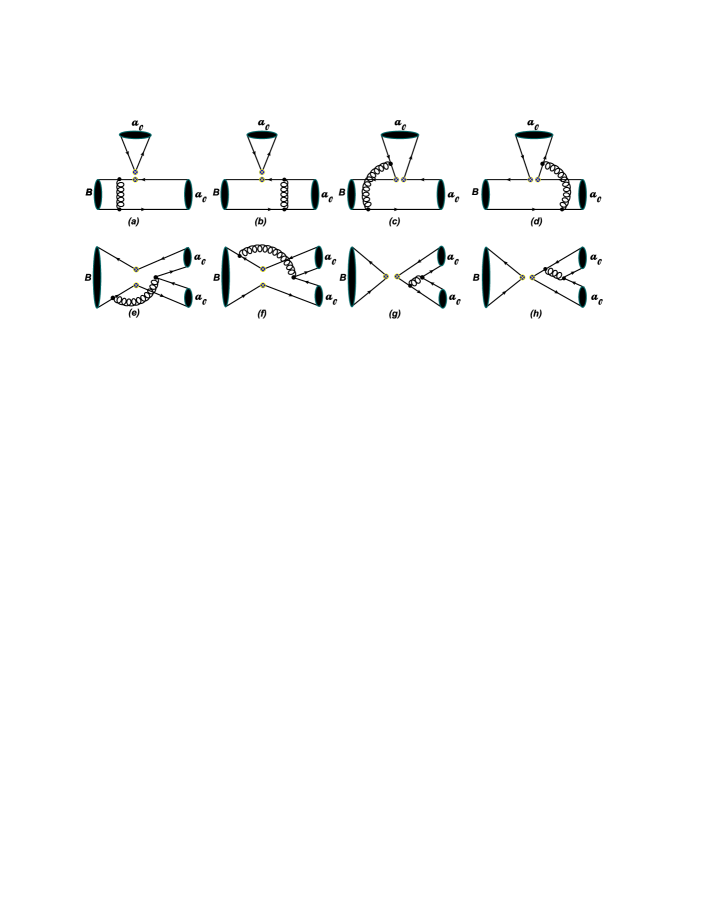
Figure 1: (Color online) Typical Feynman diagrams for $B\to a_{0}a_{0}$ decays at leading order in the pQCD approach.

Similar to $B\to\pi\pi$ decays Lu:2000em ; Li:2005kt , there are eight types of diagrams contributing to $B\to a_{0}a_{0}$ modes at leading order(LO) in the pQCD approach, as illustrated in Fig. 1. They can be classified into two types of topologies as emission and annihilation, respectively. And each kind of topology contains factorizable diagrams such as Fig. 1(a) and 1(b), in which a hard gluon connects the quarks in the same meson, and non-factorizable diagrams such as Fig. 1(c) and 1(d), in which a hard gluon attaches the quarks in two different mesons. By evaluating all these Feynman diagrams, one can obtain the decay amplitudes of $B\to a_{0}a_{0}$ decays. Because the above mentioned diagrams are the same as those in $B\to K_{0}^{*}(1430)\bar{K}_{0}^{*}(1430)$ modes Liu:2013lka , and also the light scalar mesons are considered, the formulas of $B\to a_{0}a_{0}$ decays are therefore same as those of $B\to K_{0}^{*}(1430)\bar{K}_{0}^{*}(1430)$ ones just by replacing the wave functions and input parameters correspondingly. Hence the analytic formulas for the $B\to a_{0}a_{0}$ decays are not explicitly presented in this paper.

By taking various contributions from the relevant Feynman diagrams into consideration, the total decay amplitudes for three tree-dominated $B\to a_{0}a_{0}$ channels can then be read as,

1. for $B^{0}\to a_{0}^{+}a_{0}^{-}$ decay mode,

   $${\cal A}(B^{0}\to a_{0}^{+}a_{0}^{-}) = \lambda_{u}\biggl{[}C_{1}M_{nfs}+C_{2}M_{nfa}\biggr{]}-\lambda_{t}\biggl{[}(C_{3}+C_{9})M_{nfs}+(C_{3}+2C_{4}-\frac{1}{2}(C_{9}$$ (11)

   $$-C_{10}))M_{nfa}+(C_{5}-\frac{1}{2}C_{7})M_{nfa}^{P_{1}}+(2C_{6}+\frac{1}{2}C_{8})M_{nfa}^{P_{2}}+(a_{6}-\frac{1}{2}a_{8})$$

   $$\times f_{B}F_{fa}^{P_{2}}+(a_{6}+a_{8})F_{fs}^{P2}\biggr{]}\;,$$

   where $\lambda_{u}=V_{ub}^{*}V_{ud}$ and $\lambda_{t}=V_{tb}^{*}V_{td}$. We adopt $F$ and $M$ to denote the contributions from $(V-A)(V-A)$ operators in the factorizable and non-factorizable diagrams, respectively. Analogously, $F^{P1}$ and $M^{P1}$ are chosen to denote the contributions from $(V-A)(V+A)$ operators, and $F^{P2}$ and $M^{P2}$ are taken to denote the contributions from $(S-P)(S+P)$ operators which result from the Fierz transformation of the $(V-A)(V+A)$ operators. The subscripts $fs$, $nfs$, $fa$, and $nfa$ are the abbreviations for factorizable emission, non-factorizable emission, factorizable annihilation, and non-factorizable annihilation, respectively.

2. for $B^{+}\to a_{0}^{+}a_{0}^{0}$ decay mode,

   $$\sqrt{2}{\cal A}(B^{+}\to a_{0}^{+}a_{0}^{0}) = \lambda_{u}\biggl{[}(C_{1}+C_{2})M_{nfs}\biggr{]}-\lambda_{t}\biggl{[}\frac{1}{2}(C_{7}+3C_{8})F_{fs}^{P2}+\frac{3}{2}(C_{9}+C_{10})M_{nfs}$$ (12)

   $$+\frac{3}{2}C_{8}M_{nfs}^{P_{2}}\biggr{]}\;,$$

3. for $B^{0}\to a_{0}^{0}a_{0}^{0}$ decay mode,

   $$\sqrt{2}{\cal A}(B^{0}\to a_{0}^{0}a_{0}^{0}) = \lambda_{u}\biggl{[}C_{2}(M_{nfa}-M_{nfs})\biggr{]}-\lambda_{t}\biggl{[}-(a_{6}-\frac{1}{2}a_{8})F_{fs}^{P2}+(C_{3}-\frac{1}{2}(C_{9}$$ (13)

   $$+3C_{10}))M_{nfs}-\frac{3}{2}C_{8}M_{nfs}^{P_{2}}+(C_{3}+2C_{4}-\frac{1}{2}(C_{9}-C_{10}))M_{nfa}$$

   $$+(C_{5}-\frac{1}{2}C_{7})M_{nfa}^{P_{1}}+(2C_{6}+\frac{1}{2}C_{8})M_{nfa}^{P_{2}}+(a_{6}-\frac{1}{2}a_{8})f_{B}F_{fa}^{P_{2}}\biggr{]}.$$

It is worth mentioning that the highly suppressed $F_{fs}$ has been safely neglected in all of the above decay amplitudes for the considered $B\to a_{0}a_{0}$ decays due to the either extremely small or vanishing vector decay constant. Furthermore, based on the discussions of $F_{fa}$ below Eq. (40) in Ref. Liu:2013lka , the factorizable annihilation contributions induced by the $V\pm A$ currents are therefore naturally absent because of the isospin symmetry between $u$ and $d$ quarks in the above analytical decay amplitudes.

III Numerical Results and Discussions

In this section, we will make theoretical predictions on the CP-averaged branching ratios and the CP-violating asymmetries for the $B\to a_{0}a_{0}$ decay modes considered. In numerical calculations, central values of the input parameters will be used implicitly unless otherwise stated. Firstly, we shall make several essential discussions on the input quantities.

III.1 Input quantities

For $B$ meson, the distribution amplitude in the impact $b$ space, with $b$ being the conjugate space coordinate of transverse momentum $k_{T}$, has been proposed Keum:2000ph ; Lu:2000em ; Li:2003yj ,

$$\phi_{B}(x,b) = N_{B}x^{2}(1-x)^{2}\exp\left[-\frac{1}{2}\left(\frac{xm_{B}}{\omega_{b}}\right)^{2}-\frac{\omega_{b}^{2}b^{2}}{2}\right]\;,$$ (14)

where the normalization factor $N_{B}$ is related to the decay constant $f_{B}$ through the following normalization condition,

$$\int_{0}^{1}dx\phi_{B}(x,b=0) = \frac{f_{B}}{2\sqrt{2N_{c}}}\;.$$ (15)

with the color factor $N_{c}=3$. The shape parameter $\omega_{b}$ has been fixed at $0.40$ GeV associated with $N_{B}=91.745$ by using the rich experimental data on the $B$ mesons with $f_{B}=0.19$ GeV based on lots of calculations of form factors and other well-known decay modes of $B$ meson in the pQCD approach Lu:2000em ; Keum:2000ph ; Lu:2002ny .

For the light scalar $a_{0}$, its leading twist light-cone distribution amplitude $\phi_{a_{0}}(x,\mu)$ can be generally expanded as the Gegenbauer polynomials Cheng:2005nb ; Li:2008tk :

$$\phi_{a_{0}}(x,\mu) = \frac{3}{\sqrt{2N_{c}}}x(1-x)\biggl{\{}f_{a_{0}}(\mu)+\bar{f}_{a_{0}}(\mu)\sum_{m=1}^{\infty}B_{m}(\mu)C^{3/2}_{m}(2x-1)\biggr{\}},$$ (16)

where $f_{a_{0}}(\mu)$ and $\bar{f}_{a_{0}}(\mu)$, $B_{m}(\mu)$, and $C_{m}^{3/2}(t)$ are the vector and scalar decay constants, Gegenbauer moments, and Gegenbauer polynomials, respectively. For the vector and scalar decay constants, $\bar{f}_{a_{0}}=\mu_{a_{0}}f_{a_{0}}$ with $\mu_{a_{0}}=\frac{m_{a_{0}}}{m_{2}(\mu)-m_{1}(\mu)}$ and $m_{a_{0}}=0.985$ GeV, where $m_{1}$ and $m_{2}$ are the running current quark masses in the scalar $a_{0}$. For neutral scalar $a_{0}^{0}$ meson, which cannot be produced by the vector current, the vector decay constant $f_{a_{0}^{0}}=0$ is guaranteed by charge conjugation invariance. But the quantity $\bar{f}_{a_{0}}=f_{a_{0}}\mu_{a_{0}}$ remains finite. In fact, for the charged $a_{0}^{\pm}$ meson, the vector decay constant $f_{a_{0}^{\pm}}$ also vanishes in the isospin limit. The reason is that $f_{a_{0}^{\pm}}$ is proportional to the mass difference between the constituent $d$ and $u$ quarks, which will result in $f_{a_{0}^{\pm}}$ being of order $m_{d}-m_{u}$. Hence, the contribution from the first term in Eq. (16), namely, $f_{a_{0}}$, can be neglected safely. In other words, the factorizable spectator diagrams could not contribute to $B\to a_{0}a_{0}$ decays through the vector currents. We shall use the same light-cone distribution amplitudes for both neutral and charged $a_{0}$ mesons for simplicity in this paper.

The values for scalar decay constant and Gegenbauer moments in the $a_{0}$ distribution amplitudes have been investigated at scale $\mu=1~{}\mbox{GeV}$ Cheng:2005nb :

$$\bar{f}_{a_{0}} = 0.365\pm 0.020~{}{\rm GeV},\quad B_{1}=-0.93\pm 0.10\;,\quad B_{3}=0.14\pm 0.08\;.$$ (17)

As for the twist-3 distribution amplitudes $\phi_{a_{0}}^{S}$ and $\phi_{a_{0}}^{T}$, we here adopt the asymptotic forms in our numerical calculations for simplicity Cheng:2005nb :

$$\phi^{S}_{a_{0}} = \frac{1}{2\sqrt{2N_{c}}}\bar{f}_{a_{0}},\quad\phi_{a_{0}}^{T}=\frac{1}{2\sqrt{2N_{c}}}\bar{f}_{a_{0}}(1-2x).$$ (18)

The QCD scale (GeV), masses (GeV), and $B$ meson lifetime(ps) are Keum:2000ph ; Lu:2000em ; Agashe:2014kda

$$\Lambda_{\overline{\mathrm{MS}}}^{(f=4)} = 0.250\;,\quad m_{W}=80.41\;,\quad m_{B}=5.2792\;,\quad m_{b}=4.8\;;$$

$$\tau_{B^{+}} = 1.643\;,\quad\tau_{B^{0}}=1.53\;,\quad m_{a_{0}}=0.985\;.$$ (19)

For the CKM matrix elements, we adopt the Wolfenstein parametrization and the updated parameters $A=0.814$, $\lambda=0.22537$, $\bar{\rho}=0.117\pm 0.021$, and $\bar{\eta}=0.353\pm 0.013$ Agashe:2014kda .

Utilizing the above chosen distribution amplitudes and the relevant input parameters, we can get the numerical results in the pQCD approach for the form factor $F_{0,1}^{B\to a_{0}}$  at maximal recoil as follows,

$$F_{0,1}^{B\to a_{0}}(q^{2}=0) = 0.40^{+0.05}_{-0.06}(\omega_{b})^{+0.02}_{-0.02}(\bar{f}_{a_{0}})^{+0.02}_{-0.02}(B_{i}^{a_{0}})\;,$$ (20)

where the errors arise from the shape parameter $\omega_{b}$ in $B$ meson distribution amplitude, the scalar decay constant $\bar{f}_{a_{0}}$, and the Gegenbauer moments $B_{i}^{a_{0}}(i=1,3)$ in the light $a_{0}$ distribution amplitude, respectively. This value agrees well with $0.39^{+0.10}_{-0.08}$ as given in Ref. Li:2008tk . The tiny deviation is just from the zero vector decay constant $f_{a_{0}}$ assumed in this work.

III.2 CP-averaged branching ratios and CP-violating asymmetries

In this subsection, we will analyze the CP-averaged $B\to a_{0}a_{0}$ branching ratios and the CP-violating asymmetries in the pQCD approach at LO level. For $B\to a_{0}a_{0}$ decays, the decay rate can be written as

$$\Gamma=\frac{G_{F}^{2}m^{3}_{B}}{32\pi}(1-2r_{a_{0}}^{2})|{\cal A}(B\to a_{0}a_{0})|^{2}\;,$$ (21)

where the decay amplitudes ${\cal A}$ can be referred correspondingly in Eqs. (11-13). Using the decay amplitudes obtained in last section, it is straightforward to numerically evaluate the CP-averaged branching ratios with errors as collected in Eqs. (22)-(24),

$$Br(B^{0}\to{a_{0}}^{+}{a_{0}}^{-}) = 1.5^{+0.7}_{-0.5}(\omega_{b})^{+0.3}_{-0.3}(\bar{f}_{a_{0}})^{+0.7}_{-0.6}(B_{i}^{a_{0}})^{+0.1}_{-0.1}({\rm CKM})\times 10^{-5}\;,$$ (22)

$$Br(B^{+}\to{a_{0}}^{+}{a_{0}}^{0}) = 6.1^{+2.6}_{-2.1}(\omega_{b})^{+1.4}_{-1.2}(\bar{f}_{a_{0}})^{+3.1}_{-2.2}(B_{i}^{a_{0}})^{+0.4}_{-0.4}({\rm CKM})\times 10^{-6}\;,$$ (23)

$$Br(B^{0}\to{a_{0}}^{0}{a_{0}}^{0}) = 2.7^{+1.1}_{-1.0}(\omega_{b})^{+0.6}_{-0.6}(\bar{f}_{a_{0}})^{+1.3}_{-1.0}(B_{i}^{a_{0}})^{+0.1}_{-0.2}({\rm CKM})\times 10^{-5}\;;$$ (24)

The dominant errors are induced by the uncertainties of the shape parameter $\omega_{b}=0.40\pm 0.04$ GeV for $B$ meson, the scalar decay constant $\bar{f}_{a_{0}}$, and the Gegenbauer moments $B^{a_{0}}_{i}(i=1,3)$ for the scalar $a_{0}$(see Eq. (17) for detail), respectively. It is worth stressing that the effective constraints on the above mentioned non-perturbative parameters might be helpful to explore the QCD dynamics involved in these decays and to reveal the inner structure of the light scalar $a_{0}$ state.

From Eqs. (22)-(24), one can obviously observe that the large $B\to a_{0}a_{0}$ decay rates are in the order of $10^{-6}\sim 10^{-5}$ calculated in the pQCD approach at LO level, which could be easily detected through the dominant $a_{0}$ to $\eta\pi$(or $\pi\pi)$ final state Aubert:2004hs at the running LHC and the forthcoming Super-B/Belle-II experiments. As mentioned in the Introduction, some decays involving scalar mesons were suggested as the ideal channels to test the validation of the factorization assumption Diehl:2001xe . It is therefore worth stressing that the $B^{+}\to a_{0}^{+}a_{0}^{0}$ mode would be the best choice, because it only contains a significantly suppressed factorizable emission contribution and a negligible non-factorizable emission contribution as proposed in naive factorization, but has a large branching ratio that could be easily tested in the near future experiments. Therefore, the observation of this large $B^{+}\to a_{0}^{+}a_{0}^{0}$ decay rate, on one hand, could offer an effective test to the breaking effects of the factorization assumption; on the other hand, might verify the $q\bar{q}$ components of the light scalar $a_{0}$ evidently. Furthermore, it is surprising to find that the conventionally so-called ”color-suppressed” $B^{0}\to a_{0}^{0}a_{0}^{0}$ mode has the largest branching ratio as $2.7\times 10^{-5}$, which is highly different from the known color-suppressed $B\to PP$ modes, such as the famous $B^{0}\to\pi^{0}\pi^{0}$ channel with very small branching ratio around ${\cal O}(10^{-7})$, although they embrace the same components at the quark level. Consequently, the hierarchy of the branching ratios exhibits theoretically as $Br(B^{0}\to a_{0}^{0}a_{0}^{0})\sim Br(B^{0}\to a_{0}^{+}a_{0}^{-})>Br(B^{+}\to a_{0}^{+}a_{0}^{0})$ in the pQCD approach, which is also dramatically different from that in the $B\to\pi\pi$ decays as $Br(B^{0}\to\pi^{+}\pi^{-})\gtrsim Br(B^{+}\to\pi^{+}\pi^{0})>>Br(B^{0}\to\pi^{0}\pi^{0})$ within theoretical errors Lu:2000em ; Li:2005kt ; Xiao:2011tx ; Liu:2015sra and $Br(B^{+}\to\pi^{+}\pi^{0})\gtrsim Br(B^{0}\to\pi^{+}\pi^{-})>Br(B^{0}\to\pi^{0}\pi^{0})$ within experimental uncertainties Agashe:2014kda ; Amhis:2014hma , respectively. In terms of the central values of the $B\to a_{0}a_{0}$ decay rates, the following relation can be easily found,

$$Br(B^{0}\to a_{0}^{0}a_{0}^{0}) > Br(B^{0}\to a_{0}^{+}a_{0}^{-})>Br(B^{+}\to a_{0}^{+}a_{0}^{0})\;,$$ (25)

which can be traced back to the factorization formulas as given in Eqs. (11)-(13). Specifically, the tree dominant contributions of these three decays are $C_{2}\ (M_{nfa}-M_{nfs})$, $C_{1}\ M_{nfs}+C_{2}\ M_{nfa}$, and $(C_{1}+C_{2})M_{nfs}$, respectively, in which $C_{2}$ is much larger than $C_{1}$ in magnitude with $C_{2}\sim 1.12$ and $C_{1}\sim-0.27$ at the $m_{b}$ scale, and $M_{nfs}(M_{nfa})$ stands for the amplitude of the non-factorizable emission (annihilation) diagrams induced by the tree operators $O_{1,2}$.

Table 1: The factorization decay amplitudes(in unit of $10^{-3}\;\rm{GeV}^{3}$) of the charmless hadronic $B\to a_{0}a_{0}$ decays in the pQCD approach at leading order level, where only the central values are quoted for clarification.

Decay modes	${\cal A}_{fs}$	${\cal A}_{nfs}$	${\cal A}_{nfa}$	${\cal A}_{fa}$
$B^{0}\to a_{0}^{+}a_{0}^{-}$	$\hskip 7.11317pt0.950-{\it i}0.390$	$\hskip 7.11317pt1.619-{\it i}2.982$	$-1.056-{\it i}1.876$	$-0.044+{\it i}1.212$
$B^{+}\to a_{0}^{+}a_{0}^{0}$	$-0.018+{\it i}0.007$	$-1.268+{\it i}2.926$	$0.0$	$0.0$
$B^{0}\to a_{0}^{0}a_{0}^{0}$	$\hskip 7.11317pt0.691-{\it i}0.284$	$\hskip 7.11317pt2.458-{\it i}5.100$	$-0.799-{\it i}1.363$	$-0.035+{\it i}0.853$

The underlying reason is that, as presented in Eq. (16), the asymmetric leading twist distribution amplitude $\phi_{a_{0}}(x)$ turns the originally destructive interferences induced by the symmetric one $\phi_{P}^{A}(x)$ between the two non-factorizable emission diagrams, namely, Fig. 1(c) and 1(d), in the $B\to PP$ decays into the presently constructive ones in the $B\to a_{0}a_{0}$ modes. Meanwhile, the analogous phenomenon also occurs in the annihilation topologies. Note that the values of $M_{nfa}$ are usually a bit smaller than those of $M_{nfs}$ in modulus, because the former is always power $1/m_{B}$ suppressed with $m_{B}$ being the $B$ meson mass. It is interesting to note that the QCD behavior in light scalar $a_{0}$ is greatly different from that in the pseudoscalar pion, which can be seen apparently that the leading twist $a_{0}$(pion) distribution amplitude is governed by the odd(even) Gegenbauer polynomials Cheng:2005nb ; Chernyak:1983ej ; Ball:1998tj . Therefore, large non-factorizable contributions are observed in the $B\to a_{0}a_{0}$ decays.

Table 2: Same as Table 1 but for the charmless hadronic $B\to\pi\pi$ decays.

Channels	${\cal A}_{fs}$	${\cal A}_{nfs}$	${\cal A}_{nfa}$	${\cal A}_{fa}$
$B^{0}\to\pi^{+}\pi^{-}$	$-1.845-{\it i}2.957$	$\hskip 7.11317pt0.095+{\it i}0.075$	$-0.047+{\it i}0.159$	$0.038+{\it i}0.196$
$B^{+}\to\pi^{+}\pi^{0}$	$-0.844-{\it i}1.988$	$-0.086-{\it i}0.082$	$0.0$	$0.0$
$B^{0}\to\pi^{0}\pi^{0}$	$-0.461-{\it i}0.104$	$\hskip 7.11317pt0.153+{\it i}0.135$	$-0.033+{\it i}0.113$	$0.029+{\it i}0.139$

In view of the surprisingly large $Br(B^{0}\to a_{0}^{0}a_{0}^{0})$ and the amazingly small $Br(B^{0}\to\pi^{0}\pi^{0})$ in the pQCD approach at LO level, respectively, we here present the numerical decay amplitudes(See Tables 1 and 2 for detail) arising from every topology to clarify the aforementioned predictions explicitly. It can be clearly seen that the decay amplitudes in the $B\to a_{0}a_{0}$ decays exhibit very different pattern from those in the $B\to\pi\pi$ ones, although they embrace the same diagrams at the quark level: the former modes determined by the non-factorizable contributions with a larger scalar decay constant $\bar{f}_{a_{0}}\sim 0.365$ GeV, while the latter ones dominated by the factorizable emission contributions with a smaller $f_{\pi}\sim 0.130$ GeV, apart from the special $B^{0}\to\pi^{0}\pi^{0}$ channel. As mentioned above, the underlying reason is that these considered modes include dramatically different QCD dynamics. Notice that, for the $B\to a_{0}a_{0}$ decays, because of the vanished vector decay constant $f_{a_{0}}\sim 0$, ${\cal A}_{fs}$ come only from the penguin contributions induced by the $(S+P)(S-P)$ operators, which are from the $(V+A)(V-A)$ ones by Fierz transformation. However, the phenomenologies shown in $B\to a_{0}a_{0}$ decays indicate that the famous $B\to\pi\pi$ puzzle could be resolved if a new QCD mechanism is resorted to enhance the non-factorizable contributions. Of course, it is nontrivial to resolve the $B\to\pi\pi$ puzzle just by including the large non-factorizable contributions. This point has been clarified in the literatures, for example, see Refs. Li:2009wba ; Liu:2015sra .

Because of the large errors induced by the much less constrained hadronic parameters such as the scalar decay constant $\bar{f}_{a_{0}}$, the Gegenbauer moments $B_{1}$ and $B_{3}$ in the $a_{0}$ distribution amplitudes, we derive the ratios of the branching ratios, in which the parameter uncertainties may be greatly canceled and be more helpful for measurements in the relevant experiments,

$$R_{0+} \equiv \frac{Br(B^{0}\to a_{0}^{+}a_{0}^{-})}{Br(B^{+}\to a_{0}^{+}a_{0}^{0})}\approx 2.44^{+0.06}_{-0.01}(\omega_{b})^{+0.00}_{-0.00}(\bar{f}_{a_{0}})^{+0.06}_{-0.01}(B_{i}^{a_{0}})^{+0.01}_{-0.01}({\rm CKM})\;,$$ (26)

$$R_{00} \equiv \frac{Br(B^{0}\to a_{0}^{+}a_{0}^{-})}{Br(B^{0}\to a_{0}^{0}a_{0}^{0})}\approx 0.56^{+0.01}_{-0.00}(\omega_{b})^{+0.00}_{-0.00}(\bar{f}_{a_{0}})^{+0.01}_{-0.00}(B_{i}^{a_{0}})^{+0.00}_{-0.00}({\rm CKM})\;,$$ (27)

$$R_{+0} \equiv \frac{Br(B^{+}\to a_{0}^{+}a_{0}^{0})}{Br(B^{0}\to a_{0}^{0}a_{0}^{0})}\approx 0.23^{+0.00}_{-0.00}(\omega_{b})^{+0.00}_{-0.00}(\bar{f}_{a_{0}})^{+0.00}_{-0.00}(B_{i}^{a_{0}})^{+0.00}_{-0.00}({\rm CKM})\;;$$ (28)

It is well known that the $B\to\pi\pi$ modes can provide important information to constrain the CKM unitary angle $\alpha$. As they contain the same quark diagrams as the $B\to\pi\pi$ decays, it is generally believed that the $B\to a_{0}a_{0}$ processes can also provide complementary constraints on the angle $\alpha$. Here, we show the $\alpha$ dependent branching ratios of the $B\to a_{0}a_{0}$ decays in the pQCD approach at the LO level. Based on Eqs. (11)-(13), the decay amplitudes of $B\to a_{0}a_{0}$ decays can be rewritten as follows,

$${\cal A} = V_{ub}^{*}V_{ud}T-V_{tb}^{*}V_{td}P=V_{ub}^{*}V_{ud}T(1+ze^{i(\alpha+\delta)})\;,$$ (29)

where the weak phase $\alpha=\arg\left[-\frac{V_{tb}^{*}V_{td}}{V_{ub}^{*}V_{ud}}\right]$, the ratio $z=|V_{tb}^{*}V_{td}/V_{ub}^{*}V_{ud}|\cdot|P/T|$, and $\delta$ is the relative strong phase between tree($T$) and penguin($P$) amplitudes. Correspondingly, the decay amplitudes of the $\bar{B}\to a_{0}a_{0}$ decays can be read as,

$$\overline{\cal A} = V_{ub}V_{ud}^{*}T-V_{tb}V_{td}^{*}P=V_{ub}V_{ud}^{*}T(1+ze^{i(-\alpha+\delta)})\;,$$ (30)

Therefore, the CP-averaged branching ratio of the $B\to a_{0}a_{0}$ decays shall be the following,

$$Br(B\to a_{0}a_{0}) = (|{\cal A}|^{2}+|\overline{{\cal A}}|^{2})/2=|V_{ub}^{*}V_{ud}T|^{2}(1+2z\cos\alpha\cos\delta+z^{2})\;.$$ (31)

It is thus easy to see that the CP-averaged branching ratio is a function of $\cos\alpha$ for the given ratio $z$ and the strong phase $\delta$, which can be perturbatively calculated in the pQCD approach. This gives a potential method to determine the CKM angle $\alpha$ by measuring the CP-averaged branching ratios with precision. The dependence on the CKM weak phase $\alpha$ of the CP-averaged branching ratios for $B^{0}\to a_{0}^{+}a_{0}^{-}$(Solid line), $B^{+}\to a_{0}^{+}a_{0}^{0}$(Dashed line), and $B^{0}\to a_{0}^{0}a_{0}^{0}$(Dash-dotted line) decays, respectively, are presented in Fig. 2, where the central values of the predictions in the pQCD approach are simply quoted for clarification. Then we can directly observe that the central decay rates for the $B\to a_{0}a_{0}$ decays in the pQCD approach at LO level correspond to the value around $90^{\circ}$ of the CKM angle $\alpha$, which agrees well with the constraints from various experiments Agashe:2014kda .

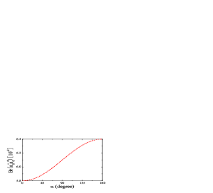
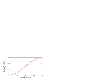
Figure 2: (Color online) Dependence on the CKM angle $\alpha$ of the $B\to a_{0}^{+}a_{0}^{-}$(Solid line), $a_{0}^{+}a_{0}^{0}$(Dashed line), and $a_{0}^{0}a_{0}^{0}$(Dash-dotted line) decay rates at leading order in the pQCD approach, respectively.

Now we turn to the evaluations of the CP-violating asymmetries of $B\to a_{0}a_{0}$ decays in the pQCD approach. For $B^{+}\to a_{0}^{+}a_{0}^{0}$ decay, the direct CP-violating asymmetry $A_{\rm CP}$ can be defined as:

$$A_{\rm CP}^{\rm dir}=\frac{|\overline{\cal A}_{f}|^{2}-|{\cal A}_{f}|^{2}}{|\overline{\cal A}_{f}|^{2}+|{\cal A}_{f}|^{2}},$$ (32)

Using Eq. (32), it is easy to calculate the direct CP-violating asymmetry for the considered $B^{+}\to a_{0}^{+}a_{0}^{0}$ mode as listed in Eq. (33),

$$A_{\rm CP}^{\rm dir}(B^{+}\to a_{0}^{+}a_{0}^{0}) = -0.6^{+0.1}_{-0.2}(\omega_{b})^{+0.1}_{-0.2}(B_{i}^{a_{0}})^{+0.0}_{-0.1}({\rm CKM})\%\;,$$ (33)

This tiny direct CP-violating asymmetry would be hard to be measured because of the extremely small penguin contributions in magnitude, although the large strong phase can be obtained due to the constructive interferences between the two non-factorizable emission diagrams with the asymmetric $a_{0}$ leading twist distribution amplitude, which is very different from that in the $B^{+}\to\pi^{+}\pi^{0}$ mode with the small non-factorizable emission contributions, relative to the purely real amplitudes from the factorizable emission diagrams in the pQCD approach at LO level.

As to the CP-violating asymmetries for the neutral decays $B^{0}\to a_{0}a_{0}$, the effects of $B^{0}-\overline{B}^{0}$ mixing should be considered. The CP-violating asymmetries of $B^{0}(\overline{B}^{0})\to{a_{0}}^{+}{a_{0}}^{-}$ and ${a_{0}}^{0}{a_{0}}^{0}$ decays are time dependent and can be defined as

$$A_{\rm CP} \equiv \frac{\Gamma\left(\overline{B}^{0}(\Delta t)\to f_{\rm CP}\right)-\Gamma\left(B^{0}(\Delta t)\to f_{\rm CP}\right)}{\Gamma\left(\overline{B}^{0}(\Delta t)\to f_{\rm CP}\right)+\Gamma\left(B^{0}(\Delta t)\to f_{\rm CP}\right)}$$ (34)

$$= A_{\rm CP}^{\rm dir}\cos(\Delta m\Delta t)+A_{\rm CP}^{\rm mix}\sin(\Delta m\Delta t),$$

where $\Delta m$ is the mass difference between the two $B_{d}^{0}$ mass eigenstates, $\Delta t=t_{\rm CP}-t_{tag}$ is the time difference between the tagged $B^{0}$ ($\overline{B}^{0}$) and the accompanying $\overline{B}^{0}$ ($B^{0}$) with opposite $b$ flavor decaying to the final CP-eigenstate $f_{\rm CP}$ at the time $t_{\rm CP}$. The direct- and mixing-induced CP-violating asymmetries $A_{\rm CP}^{\rm dir}$ and $A_{\rm CP}^{\rm mix}$ can be written as

$$A_{\rm CP}^{\rm dir}=\frac{\left|\lambda_{\rm CP}\right|^{2}-1}{1+|\lambda_{\rm CP}|^{2}},\quad A_{\rm CP}^{\rm mix}=\frac{2{\rm Im}(\lambda_{\rm CP})}{1+|\lambda_{\rm CP}|^{2}},$$ (35)

with the CP-violating parameter $\lambda_{\rm CP}$

$$\lambda_{\rm CP} \equiv \eta_{f}\;\frac{V_{tb}^{*}V_{td}}{V_{tb}V_{td}^{*}}\cdot\frac{\langle f_{\rm CP}|H_{eff}|\overline{B}^{0}\rangle}{\langle f_{\rm CP}|H_{eff}|B^{0}\rangle}.$$ (36)

where $\eta_{f}$ is the CP-eigenvalue of the final states. Then the direct- and mixing-induced CP-violating asymmetries for the $B^{0}\to a_{0}^{+}a_{0}^{-}$ and $a_{0}^{0}a_{0}^{0}$ decays in the pQCD approach at LO level can be calculated as,

$$A_{\rm CP}^{\rm dir}(B^{0}\to a_{0}^{+}a_{0}^{-}) = 31.0^{+3.7}_{-2.3}(\omega_{b})^{+10.4}_{-8.7}(B_{i}^{a_{0}})^{+1.4}_{-1.4}({\rm CKM})\%\;,$$ (37)

$$A_{\rm CP}^{\rm mix}(B^{0}\to a_{0}^{+}a_{0}^{-}) = 0.9^{+9.2}_{-7.3}(\omega_{b})^{+7.4}_{-9.2}(B_{i}^{a_{0}})^{+9.8}_{-9.6}({\rm CKM})\%\;,$$ (38)

$$A_{\rm CP}^{\rm dir}(B^{0}\to a_{0}^{0}a_{0}^{0}) = 16.2^{+1.7}_{-1.1}(\omega_{b})^{+5.9}_{-4.9}(B_{i}^{a_{0}})^{+0.7}_{-0.9}({\rm CKM})\%\;,$$ (39)

$$A_{\rm CP}^{\rm mix}(B^{0}\to a_{0}^{0}a_{0}^{0}) = 4.6^{+4.9}_{-3.6}(\omega_{b})^{+4.3}_{-4.8}(B_{i}^{a_{0}})^{+9.9}_{-9.8}({\rm CKM})\%\;,$$ (40)

where we have neglected the vanishing theoretical errors for the CP-violations in $B\to a_{0}a_{0}$ decays arising from the scalar decay constant $\bar{f}_{a_{0}}$ of $a_{0}$ meson. It is interesting to see that these two channels, namely, $B^{0}\to a_{0}^{+}a_{0}^{-}$ and $B^{0}\to a_{0}^{0}a_{0}^{0}$, have large branching ratios and large direct CP asymmetries simultaneously, which could be easier to be measured at the running LHC experiments and the forthcoming Super-B/Belle-II factory, and have the potential to reveal the QCD dynamics and the inner structure involved in the light scalar $a_{0}$ meson.

Similarly, based on Eqs. (29), (30), and (33), the direct CP-violating asymmetry can also be expressed as the function of the CKM angle $\alpha$,

$$A_{\rm CP}^{\rm dir} = \frac{2z\sin\alpha\sin\delta}{1+2z\cos\alpha\cos\delta+z^{2}}\;.$$ (41)

Then the precise measurements on these large direct CP violations can also provide the constraints on the CKM angle $\alpha$ potentially. The variation of the direct CP-violating asymmetries with the CKM angle $\alpha$ for the $B^{0}\to a_{0}^{+}a_{0}^{-}$(Solid line) and $a_{0}^{0}a_{0}^{0}$(Dashed line) decays is shown in Fig. 3. Again, the central value about $90^{\circ}$ of the CKM angle $\alpha$ can be utilized to produce the above mentioned large direct CP violations.

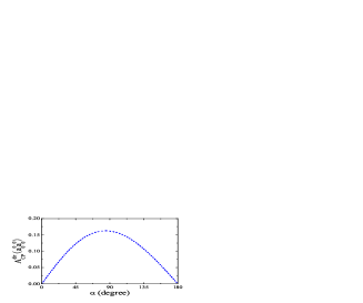
Figure 3: (Color online) Dependence on the CKM angle $\alpha$ of the $B\to a_{0}^{+}a_{0}^{-}$(Solid line) and $a_{0}^{0}a_{0}^{0}$(Dashed line) direct CP violations at leading order in the pQCD approach, respectively.

IV Summary

In summary, we studied the two-body charmless hadronic $B\to a_{0}a_{0}$ decays, which have the same Feynman diagrams as the $B\to\pi\pi$ modes at the quark level, by employing the pQCD factorization approach based on the $k_{T}$ factorization theorem. Based on the assumption of two-quark($q\bar{q}$) structure of the light scalar $a_{0}$ state, we make theoretical predictions on the CP-averaged branching ratios and the CP-violating asymmetries of the considered $B\to a_{0}a_{0}$ channels in the SM. Due to the large non-factorizable contributions induced by the asymmetric leading twist distribution amplitude of $a_{0}$ meson, large branching ratios in the order of $10^{-6}\sim 10^{-5}$ have been predicted in the pQCD approach at LO level. At the same time, large direct CP violations around $15\%$ and $30\%$ in the $B^{0}\to a_{0}^{0}a_{0}^{0}$ and $a_{0}^{+}a_{0}^{-}$ decays have also been observed. It is therefore expected that the large branching ratios plus the large CP asymmetries would be easier to be measured at the running LHC experiments and the forthcoming Super-B/Belle-II factory, if $a_{0}$ is indeed the $q\bar{q}$ bound state. Furthermore, the large non-factorizable contributions in the $B\to a_{0}a_{0}$ decays can hint some important information on resolving the famous $B\to\pi\pi$ puzzle, although this is non-trivial work as clarified in the literatures Li:2009wba ; Liu:2015sra . The detection of these considered decays might be helpful to investigate the QCD dynamics in the channels and to explore the inner structure of the light scalar $a_{0}$ state. The investigation of the $B\to a_{0}a_{0}$ decays could also provide more complementary constraints on the CKM weak phase $\alpha$, since the same components as the $B\to\pi\pi$ modes exist in the considered $B\to a_{0}a_{0}$ ones at the quark level. Frankly speaking, the predictions in the present work suffered from large uncertainties induced by the much less constrained hadronic parameters such as the Gegenbauer moments $B_{1}^{a_{0}}$ and $B_{3}^{a_{0}}$, which need further studies in the non-perturbative QCD(such as QCD sum rule and/or Lattice QCD) calculations and the relevant experimental measurements(e.g., at BESIII, LHC, Super-B/Belle-II, etc.) on the productions and/or decays involving the $a_{0}$ state.

- (1) K. A. Olive et al. [Particle Data Group Collaboration], Chin. Phys. C 38, 090001 (2014).
- (2) Y. Amhis et al. [Heavy Flavor Averaging Group Collaboration], arXiv:1412.7515; updated in http://www.slac.stanford.edu/xorg/hfag.
- (3) T. Gershon and A. Soni, J. Phys. G 34, 479 (2007).
- (4) M. Bona et al. [SuperB Collaboration], arXiv:0709.0451 [hep-ex]; T. Aushev et al. [Belle-II Collaboration], arXiv:1002.5012 [hep-ex].
- (5) Y. Y. Keum, H.-n. Li, and A. I. Sanda, Phys. Lett. B 504, 6 (2001); Phys. Rev. D 63, 054008 (2001).
- (6) C. D. Lü, K. Ukai, and M. Z. Yang, Phys. Rev. D 63, 074009 (2001).
- (7) H.-n. Li, Prog. Part. Nucl. Phys. 51, 85 (2003).
- (8) G. Buchalla, A.J. Buras, and M.E. Lautenbacher, Rev. Mod. Phys. 68, 1125 (1996).
- (9) X. Liu, Z. J. Xiao and Z. T. Zou, J. Phys. G 40, 025002 (2013).
- (10) H. Y. Cheng, C. K. Chua, and K. C. Yang, Phys. Rev. D 73, 014017 (2006); ibid. 77, 014034 (2008).
- (11) H. Y. Cheng and J. G. Smith, Ann. Rev. Nucl. Part. Sci. 59, 215 (2009).
- (12) X. Liu, H.-n. Li and Z. J. Xiao, Phys. Rev. D 91, 114019 (2015).
- (13) M. Bauer, B. Stech and M. Wirbel, Z. Phys. C 34, 103 (1987); M. Wirbel, B. Stech and M. Bauer, Z. Phys. C 29, 637 (1985).
- (14) M. Diehl and G. Hiller, J. High Energy Phys. 06, 067 (2001); S. Laplace and V. Shelkov, Eur. Phys. J. C 22, 431 (2001).
- (15) M. Beneke, G. Buchalla, M. Neubert and C. T. Sachrajda, Phys. Rev. Lett. 83, 1914 (1999); Nucl. Phys. B 591, 313 (2000).
- (16) D. s. Du, D. s. Yang and G. h. Zhu, Phys. Lett. B 488, 46 (2000).
- (17) H.-n. Li, Phys. Rev. D 55, 105 (1997); Phys. Lett. B 405, 347 (1997).
- (18) C. W. Bauer, D. Pirjol, I. Z. Rothstein and I. W. Stewart, Phys. Rev. D 70, 054015 (2004).
- (19) C.M. Arnesen, Z. Ligeti, I.Z. Rothstein, and I.W. Stewart, Phys. Rev. D 77, 054006 (2008).
- (20) J. Chay, H.-n. Li, and S. Mishima, Phys. Rev. D 78, 034037 (2008).
- (21) C.D. Lü and K. Ukai, Eur. Phys. J. C 28, 305 (2003).
- (22) Y. Li, C.D. Lü, Z.J. Xiao, and X.Q. Yu, Phys. Rev. D 70, 034009 (2004).
- (23) A. Ali, G. Kramer, Y. Li, C.D. Lü, Y.L. Shen, W. Wang, and Y.M. Wang, Phys. Rev. D 76, 074018 (2007).
- (24) Z.J. Xiao, W.F. Wang, and Y.Y. Fan, Phys. Rev. D 85, 094003 (2012); Y.L. Zhang, X.Y. Liu, Y.Y. Fan, S. Cheng, and Z.J. Xiao, Phys. Rev. D 90, 014029 (2014).
- (25) H.-n. Li, S. Mishima, and A. I. Sanda, Phys. Rev. D 72, 114005 (2005).
- (26) C. D. Lü and M. Z. Yang, Eur. Phys. J. C 28, 515 (2003).
- (27) R. H. Li, C. D. Lü, W. Wang and X. X. Wang, Phys. Rev. D 79, 014013 (2009).
- (28) B. Aubert et al. [BaBar Collaboration], Phys. Rev. D 70, 111102 (2004); ibid. 75, 111102 (2007); S. Uehara et al. [Belle Collaboration], Phys. Rev. D 80, 032001 (2009); R. Aaij et al. [LHCb Collaboration], Phys. Rev. D 88, 072005 (2013).
- (29) V. L. Chernyak and A. R. Zhitnitsky, Phys. Rept. 112, 173 (1984); A. R. Zhitnitsky, I. R. Zhitnitsky and V. L. Chernyak, Sov. J. Nucl. Phys. 41, 284 (1985) [Yad. Fiz. 41, 445 (1985)]; V. M. Braun and I. E. Filyanov, Z. Phys. C 44, 157 (1989) [Sov. J. Nucl. Phys. 50, 511 (1989)] [Yad. Fiz. 50, 818 (1989)]; V. M. Braun and I. E. Filyanov, Z. Phys. C 48, 239 (1990) [Sov. J. Nucl. Phys. 52, 126 (1990)] [Yad. Fiz. 52, 199 (1990)].
- (30) P. Ball, J. High Energy Phys. 09, 005 (1998); P. Ball, J. High Energy Phys. 01, 010 (1999).
- (31) H.-n. Li and S. Mishima, Phys. Rev. D 83, 034023 (2011); ibid. 90, 074018 (2014).