Optimal fidelity of teleportation with continuous-variable using three-tunable parameters in realistic environment

Abstract

We introduce three tunable parameters to optimize the fidelity of quantum teleportation with continuous-variable in nonideal scheme. Using the characteristic function formalism, we present the condition that the teleportation fidelity is independent of the amplitude of input coherent states for any entangled resource. Then we investigate the effects of tunable parameters on the fidelity with or without the presence of environment and imperfect measurements, by analytically deriving the expression of fidelity for three different input coherent state distributions. It is shown that, for the linear distribution, the optimization with three tunable parameters is the best one with respect to single- and two-parameter optimization. Our results reveal the usefulness of tunable parameters for improving the fidelity of teleportation and the ability against the decoherence.

PACS number(s): 03.65 -a. 42.50.Dv

I Introduction

Quantum teleportation has an indispensable role in the manipulation of quantum states and processing of quantum information 1 ; 2 ; 3 ; 3a . Usually, the two-mode squeezed vacuum is often used as the entanglement resource with continuous-variable (CV). However, due to the limit of experiment, it is hard to achieve high degree of squeezing which leads to a low effect of teleportation fidelity.

In order to increase the entanglement and fidelity of teleportation, a number of stratigies have been proposed 4 ; 5 ; 6 ; 7 ; 8 ; 9 ; 10 ; 11 ; 12 ; 13 . Among them, non-Gaussian operations including the photon subtraction $a$ or addition $a^{{\dagger}}$ or the superposition of both can be used to realize this purpose for given Vaidman-Brauntein-Kimble (VBK) scheme. For example, the superposition operator $ta^{{\dagger}}+ra$ is proposed for quantum state engineering to transform a classical state to a nonclassical one 14 , and then is performed on two-mode squeezed vacuum (TMSV) for enhancing quantum entanglement as well as the fidelity of teleportation 15 . It is found that the fidelity teleporting coherent state can be further improved by optimizing the superposition operation compared with the other non-Gaussian states, such as photon-subtraction TMSV. As another example, a remarkable improvement of the teleportation fidelity with CV can be obtained by introducing another optimal non-Gaussian resources when given the usual and (non-)ideal VBK scheme 16 ; 17 ; 18 by considering imperfect Bell measurements and damping. In Ref. 18, the “shot-fidelity” and single-gain factor are used to discuss the performance of teleportation. In fact, these protocols above are employed to enhance the fidelity of teleportation by changing quantum entangled resources.

Then an inverse question is that given a certain class of entangled resources with some given properties, how we can modify the VBK scheme to improve the fidelity of teleportation. It is interesting to notice that there is an alternative method to improve the fidelity of teleportation by using calssical information. For instance, the teleportation fidelity of CV can be enhanced by tuning the gain in the measurement dependent modulation on the output field 6 ; 19 in Heisenberg picture and EPR resources without loss, which has been realized experimentally by Furusawa et al 20 . However, these two important theoretical works are concerned with the study of the ideal protocol implementation using Gaussian resources 6 ; 19 . In addition, there are some other strategies of gain tuning and of optimal gain 21 ; 22 , using the Heisenberg picture and the Wigner function, but they can not be directly applied to more general cases. In addition, in Refs. 21 ; 23 the gain factor is used to maximize the teleportation fidelity for the case of Gaussian resources, but the gain-optimized fidelity of teleportation is strongly suppressed when considered the dissipation. Recently, a hybrid entanglement swapping protocol is proposed experimentally to transfer discrete-variable (DV) entanglement by using continuous-variable (CV) Gaussian entangled resources and by tuning a gain factor of the teleporter 22 ; 24 ; 25 , which shows that DV entanglement remains present after teleportation for any squeezing by optimal gain tuning. For more information about advances in quantum teleportation, we refer to a recent review paper 26 and references therein.

The fidelity of teleportation, as mentioned above, can be improved by using tunable entangled resources or classical parameters 16 ; 17 ; 19 ; 22 . In Ref. 19 , a three-parameter optimal stratigy is introduced to improve the quality of teleporttaion, including unbalanced beam splitter (BS) and two non-unity gains. However, they only considered an ideal case. Actually, the interaction between quantum system and environment can not be avoided and Bell measurements are usually imperfect. Thus, it would be interesting that whether it is still effective to enhance the fidelity by using these tunable parameters in realistic case. In this paper, using the characteristics function (CF) formalism, we shall extend the analysis of the parameter optimization strategy for realistic input states and non-ideal entangled resources and investigate the nonideal quantum teleportation by deriving an analytical expression of the teleportation fidelity. This formalism is very convenient to discuss the teleportation for the nonideal case and any entangled resources. As far as we know, there is no related report up to now.

This paper is arranged as following. In Sec. II, we give a description of the characteristic function formulism for the case of nonideal parameterized teleportation with CV scheme. In this scheme, we find the condition that the fidelity is independent of the amplitude of input coherent states for any entangled resource. And then we present a qualitative description about fidelity and average fidelity. In Sec. III, we derive the analytical expression of the fidelity of teleportation when the TMSV and coherent states are used as entangled channel and teleported states, respectively. In Sec. IV we study the performance of amplitude-independent optimal fidelity using the condition found in Sec. II. It is found that the optimal condition is just that the two-gain factors and $\theta$ are equal to unit and $\pi/4$, respectively. Sec. V is devoted to discussing the optimal fidelity over these three tunable parameters and three different probability distributions for the input coherent states by deriving the analytical expression of the optimal fidelity. Our conclusions are drawn in the last section.

II Mode and quantitative analysis

Here, we consider a more realistic case of teleportation scheme shown in Fig. 1(a). In this scheme, there are three tunable parameters, unbanlanced BS and two non-unity gains ($g_{q}$ and $g_{p}$). The input state (mode 1) and the entangled resources (shared by modes 2 and 3) are not limited to be pure states. Considering that the mode 2 can be prepared close to the sender Alice while the mode 3 usually has to propagate over much longer distance, we can assume that the mode 2 is not affected by losses but the mode 3 is. In addition, two symmetrical lossy bosonic channel have been considered before making Bell measurements, which are simulated through an extra vacuum mode and a beam splitter with transmission coefficient $T$. The input states of modes 4 and 5 are pure vacuum states.

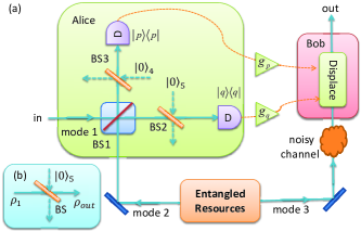
Figure 1: (Colour online) Realistic schematic diagram for CV teleportation. BS: Beam splitter.

Next, we shall give a description about the scheme in the formalism of CF where it is very convenient to discuss the teleportation for the nonideal case and non-Gaussian entangled resourecs 17 ; 27 .

II.1 The input-output relation of BS in CF formalism

In order to obtain the relation between input and output, we first calculate the output of a beam splitter with a vacuum and an arbitrary density operator as inputs shown in Fig. 1(b). For simplicity, we denote the vacuum and the input state as $\left|0\right\rangle_{5}$ and $\rho_{1}$, respectively. The output state (denoted as $\rho_{1}^{\prime}$) is given by

$$\rho_{1}^{\prime}=\text{Tr}_{5}\left[B_{15}\left(T\right)\rho_{1}\otimes\left|0\right\rangle_{5,5}\left\langle 0\right|B_{15}^{{\dagger}}\left(T\right)\right],$$ (1)

where Tr₅ is the partial trace over the ancilla mode 5 and $B_{kl}\left(T\right)=\exp[\varphi(a_{k}a_{l}^{{\dagger}}-a_{k}^{{\dagger}}a_{l})]$ is the beam splitter operator describing the interaction between modes 1 and 5 with $\cos\varphi=\sqrt{T}$ and $a_{k,l}$ ($k=1,l=5$) being the photon annihilation operator of the $k(l)-$modes. Using the Weyl expansion of density operator, we can express the density operator $\rho_{1}$ and the vacuum projector $\left|0\right\rangle_{55}\left\langle 0\right|$ as the following forms:

$$\rho_{1} ={\displaystyle\int}\frac{d^{2}\alpha}{\pi}\chi_{1}\left(\alpha\right)D_{1}\left(-\alpha\right),$$

$$\left|0\right\rangle_{55}\left\langle 0\right| ={\displaystyle\int}\frac{d^{2}\beta}{\pi}e^{-\frac{1}{2}\left|\beta\right|^{2}}D_{5}\left(-\beta\right),$$ (2)

where $D_{1}\left(\alpha\right)=\exp\{\alpha a_{1}^{{\dagger}}-\alpha^{\ast}a_{1}\}$ is the displacement operator, and $\chi_{1}\left(\alpha\right)$ is the CF of $\rho_{1}$. On the other hand, using the following transformation relation

$$B_{15}D_{1}\left(-\alpha\right)D_{5}\left(-\beta\right)B_{15}^{{\dagger}}=D_{1}\left(\bar{\alpha}\right)D_{5}\left(\bar{\beta}\right),$$ (3)

where $R=1-T$, and $\bar{\alpha}=\beta\sqrt{R}-\alpha\sqrt{T},\bar{\beta}=-\beta\sqrt{T}-\alpha\sqrt{R}$, we can derive

$$\text{Tr}_{5}\left[B_{15}D_{1}\left(-\alpha\right)D_{5}\left(-\beta\right)B_{15}^{{\dagger}}\right]$$

$$=D_{1}\left(\bar{\alpha}\right)\text{Tr}_{5}\left[D_{5}\left(\bar{\beta}\right)\right]$$

$$=D_{1}\left(\bar{\alpha}\right)\pi\delta^{(2)}(\bar{\beta}).$$ (4)

Here we have used the relation Tr${}_{5}D_{5}(\bar{\beta})=\pi\delta^{(2)}(\bar{\beta})$. Then substituting Eqs. (2) and (4) into Eq. (1) yields

$$\rho_{1}^{\prime} ={\displaystyle\int}\frac{d^{2}\alpha d^{2}\beta}{\pi^{2}}e^{-\frac{1}{2}\left|\beta\right|^{2}}\chi_{1}\left(\alpha\right)\text{Tr}_{5}\left[D_{1}\left(\bar{\alpha}\right)D_{5}\left(\bar{\beta}\right)\right]$$

$$={\displaystyle\int}\frac{d^{2}\alpha d^{2}\beta}{\pi^{2}}e^{-\frac{1}{2}\left|\beta\right|^{2}}\chi_{1}\left(\alpha\right)D_{1}\left(\bar{\alpha}\right)\pi\delta^{(2)}\left(\bar{\beta}\right)$$

$$={\displaystyle\int}\frac{d^{2}\alpha}{\pi}e^{-\frac{1}{2}R\left|\alpha\right|^{2}}\chi_{1}\left(\sqrt{T}\alpha\right)D_{1}\left(-\alpha\right),$$ (5)

where $e^{-\frac{1}{2}\left|\beta\right|^{2}}$ is the CF of the vacuum state, and in the second step in Eq. (5) the CF $\chi_{1}\left(\alpha\right)$ is transformed to $\chi_{1}(\sqrt{T}\alpha)$ with a Gaussian term $e^{-\frac{1}{2}R\left|\alpha\right|^{2}}$ due to the photon loss. It is then convenient to obtain the input-output relation of the teleportation scheme shown in Fig. 1(a) as follows.

II.2 The input-output relation of the teleportation scheme in CF formalism including photon-loss or imperfect Bell measurements

Now, we consider the effect of photon-loss on the relation between input and output of the teleportation scheme in CF formalism. Here we use BS2 and BS3 with vacuum inputs to simulate the photon loss or imperfect Bell measurements (see Fig. 1(b)), and denote the teleported state, entangled resource, and auxiliary vacuum as $\rho_{1},$ $\rho_{23}$ and $\left|00\right\rangle_{45}$, respectively. In oder to realize the teleportation, Alice shall make her Bell measurements. Before she does, the unitary state evolution can be formulated as

$$\rho_{1-5}=U\otimes\rho_{1}\otimes\rho_{23}\otimes\left|00\right\rangle_{45}\left\langle 00\right|U^{\dagger},$$ (6)

where the unitary evolution operator is defined as $U\left.=\right.B_{24}B_{15}B_{12}$ and $B_{kl}$ are the BS operator defined before. In a similar way to deriving Eq. (5), and using the Weyl expansion for the entangled resource, the reduced output state denoted as $\rho_{1-3}\equiv$Tr${}_{45}\rho_{1-5}$ is given by

$$\rho_{1-3} =\text{Tr}_{45}\left[U\otimes\rho_{1}\otimes\rho_{23}\otimes\left|00\right\rangle_{45}\left\langle 00\right|U^{\dagger}\right]$$

$$={\displaystyle\int}\frac{d^{2}\alpha d^{2}\beta d^{2}\gamma}{\pi^{3}}\chi_{1}\left(\alpha\right)\chi_{23}\left(\beta,\gamma\right)$$

$$\times\text{Tr}_{45}\left[UD_{1}\left(-\alpha\right)D_{2}\left(-\beta\right)D_{3}\left(-\gamma\right)\left|00\right\rangle_{45}\left\langle 00\right|U^{\dagger}\right]$$

$$={\displaystyle\int}\frac{d^{2}\alpha d^{2}\beta d^{2}\gamma}{\pi^{3}}\chi_{1}\left(\alpha\right)\chi_{23}\left(\beta,\gamma\right)\text{Tr}_{45}[B_{24}$$

$$\times B_{15}D_{1}(-\alpha_{1})D_{2}(-\beta_{1})D_{3}\left(-\gamma\right)\left|00\right\rangle_{45}\left\langle 00\right|B_{24}^{\dagger}B_{15}^{\dagger}],$$ (7)

where $B_{12}D_{1}\left(-\alpha\right)D_{2}\left(-\beta\right)B_{12}^{{\dagger}}=D_{1}(-\alpha_{1})D_{2}(-\beta_{1})$ with $\alpha_{1}=\alpha\cos\theta-\beta\sin\theta$, $\beta_{1}=\beta\cos\theta+\alpha\sin\theta$ and $\cos^{2}\theta$ being the transmission coefficient of beam splitter $B_{12}$. Using Eq. (1) and (4), we can obtain

$$\rho_{1-3} ={\displaystyle\int}\frac{d^{2}\alpha d^{2}\beta d^{2}\gamma}{\pi^{3}}\chi_{1}(\sqrt{T}\alpha)\chi_{23}(\sqrt{T}\beta,\gamma)$$

$$\times e^{-\frac{R}{2}(\left|\alpha_{1}\right|^{2}+\left|\beta_{1}\right|^{2})}D_{1}\left(-\alpha_{1}\right)D_{2}\left(-\beta_{1}\right)D_{3}\left(-\gamma\right).$$ (8)

Eq. (8) is the representation in CF of deduced density operator before Bell measurements but after BS2 and BS3.

Then, as the first step of teleportation, Alice makes a joint measurements for modes 1 and 2 at the output ports, i.e., measures two observables corresponding to coordinate and momentum of modes 1 and 2. Thus after the measurements, the outcomes $\rho_{M}$ ($M$ means measurement) in mode 3 are

$$\rho_{M}\equiv\frac{1}{P\left(q,p\right)}\text{Tr}_{12}\left[\left|q\right\rangle_{11}\left\langle q\right|\otimes\left|p\right\rangle_{22}\left\langle p\right|\rho_{1-3}\right],$$ (9)

where $P\left(q,p\right)$ is the probability distribution function of the Bell measurement outcomes, $P\left(q,p\right)=$Tr${}_{3}\{$Tr${}_{12}[\left|q\right\rangle_{11}\left\langle q\right|\otimes\left|p\right\rangle_{22}\left\langle p\right|\rho_{1-3}]\}$, and $\left|q\right\rangle_{1}\$and $\left|p\right\rangle_{2}$ are the eigenstates of coordinate and momentum operators $Q_{1}$ and $P_{2}$ corresponding to modes 1 and 3, respectively.

According to the definition of CF, and using the following relations

$$\text{Tr}_{1}\left[\left|q\right\rangle_{1,1}\left\langle q\right|D_{1}\left(\alpha\right)\right] =e^{i\sqrt{2}q\operatorname{Im}\alpha}\delta\left(\sqrt{2}\operatorname{Re}\alpha\right),$$

$$\text{Tr}_{2}\left[\left|p\right\rangle_{2,2}\left\langle p\right|D_{2}\left(\beta\right)\right] =e^{-i\sqrt{2}p\operatorname{Re}\beta}\delta\left(\sqrt{2}\operatorname{Im}\beta\right),$$ (10)

and

$$\text{Tr}_{3}\left[D_{3}\left(-\gamma\right)D_{3}\left(\eta\right)\right]=\pi\delta^{(2)}\left(\eta-\gamma\right),$$ (11)

the CF of $\rho_{M}$ defined as $\chi_{M}\left(q,p;\eta\right)$=Tr${}_{3}\left[\rho_{M}D_{3}\left(\eta\right)\right]$ reads

$$\chi_{M}\left(q,p;\eta\right)$$

$$=\frac{P^{-1}\left(q,p\right)}{\sin 2\theta}{\displaystyle\int}\frac{d^{2}\alpha}{\pi^{2}}\exp\left\{\alpha^{\ast}\xi-\alpha\xi^{\ast}\right\}$$

$$\times\chi_{1}(\sqrt{T}\alpha)\chi_{23}\left[\sqrt{T}\left(\alpha\cot 2\theta+\alpha^{\ast}\csc 2\theta\right),\eta\right]$$

$$\times\exp\left\{-\frac{R}{2}[(\operatorname{Re}\alpha)^{2}\csc^{2}\theta+(\operatorname{Im}\alpha)^{2}\sec^{2}\theta]\right\},$$ (12)

where we have defined $\xi=(q/\cos\theta+ip/\sin\theta)/\sqrt{2}$. When $T=1$, Eq. (12) just reduces to Eq.(2.9) in Ref. 27 .

After Alice informs the measured results ($q,p$) to Bob, Bob needs to make a unitary transformation to obtain the output state at this stage. Here, we consider the unitary transformation to be the displacement operator $D_{3}\left(Z\right)$ with non-nunity and aysmetrical gains characteristic, where $Z\equiv g_{q}q+ig_{p}p$ with $g_{q}$ and $g_{p}$ are two tunable gain parameters. Thus, after the displacement, the output state can be expressed as $\rho_{D}\equiv\int d^{2}\eta\chi_{M}\left(q,p;\eta\right)D_{3}\left(Z\right)D_{3}\left(-\eta\right)D_{3}\left(-Z\right)/\pi$. Usually, we do not have interest in every measurement result but the average effect. Thus we perform an ensemble averaging over all measurement results, then the average CF $\bar{\chi}_{out}$ is given by

$$\bar{\chi}_{out}\left(\beta\right) =\text{Tr}_{3}[D_{3}\left(\beta\right)\int dqdpP\left(q,p\right)\rho_{D}]$$

$$=\chi_{1}\left(f_{1}\beta-f_{2}\beta^{\ast}\right)\chi_{23}\left(\beta^{\ast}f_{3}-\beta\allowbreak f_{4},\beta\right)$$

$$\times\exp\{-R[g_{p}^{2}(\operatorname{Re}\beta)^{2}+g_{q}^{2}(\operatorname{Im}\beta)^{2}]\},$$ (13)

where

$$f_{1} =\sqrt{\frac{T}{2}}\left(g_{q}\cos\theta+g_{p}\sin\theta\right),$$

$$f_{2} =\sqrt{\frac{T}{2}}\left(g_{q}\cos\theta-g_{p}\sin\theta\right),$$

$$f_{3} =\sqrt{\frac{T}{2}}\left(g_{q}\sin\theta+g_{p}\cos\theta\right),$$

$$f_{4} =\sqrt{\frac{T}{2}}\left(g_{q}\sin\theta-g_{p}\cos\theta\right),$$ (14)

and $T$ and $R$ ($T+R=1$) denote, respectively, the transmissivity and reflectivity of the BS2 and BS3 that stimulate the photon losses.

II.3 Relation between input and output including noise in mode 3

Next, we consider the effect in CF formalism of decoherence of environment on the mode 3. Here we consider the case that the mode 3 propagates in a noisy channel such as photon loss, and thermal noise after Alice’s measurement but before its reaching Bob’s location (see Fig. 1(a)). In the interaction picture and the Born-Markov approximation, the time evolution of the density matrix describing the thermal environment is governed by the master equation (ME) 28 :

$$\frac{d}{dt}\rho\left(t\right) =\kappa\bar{n}\left(2a^{{\dagger}}\rho a-aa^{{\dagger}}\rho-\rho aa^{{\dagger}}\right)$$

$$+\kappa\left(\bar{n}+1\right)\left(2a\rho a^{{\dagger}}-a^{{\dagger}}a\rho-\rho a^{{\dagger}}a\right),$$ (15)

where $\kappa$ and $\bar{n}$ are the dissipative coefficient and the average thermal photon number of the environment, respectively. When $\bar{n}=0,$ Eq. (15) reduces to the one describing the photon-loss channel. By solving the ME in the CF form, one can find that the evolution of CF described by Eq. (15) is given by

$$\chi\left(\gamma;t\right)=\chi\left(\gamma e^{-\kappa t};0\right)\exp\left\{-\Gamma\left|\gamma\right|^{2}\right\},$$ (16)

where $\Gamma=\left(2\bar{n}+1\right)\left(1-e^{-2\kappa t}\right)/2$, and $\chi\left(\gamma;0\right)$ is the CF of initial state $\rho\left(0\right)$. In a similar way to deriving Eq. (13), at Bob’s location, the CF $\bar{\chi}_{f}$ of final output state for the teleportation scheme can be directly given by

$$\bar{\chi}_{f}\left(\beta;t\right) =e^{-\Gamma\left|\beta\right|^{2}}\chi_{1}\left(f_{1}\beta-f_{2}\beta^{\ast}\right)$$

$$\times\chi_{23}\left(\beta^{\ast}f_{3}-\beta\allowbreak f_{4},\beta e^{-\kappa t}\right)$$

$$\times\exp\{-R[g_{p}^{2}(\operatorname{Re}\beta)^{2}+g_{q}^{2}(\operatorname{Im}\beta)^{2}]\}.$$ (17)

The form of Eq. (17) shows the different roles played by the noise channel ($\Gamma,\kappa$) and gain factors ($g_{p},g_{q}$) as well as unbalanced BS ($\theta$), the reflectivity $R$. The decoherence effect from the noisy channel affects only mode 3 by means of the exponentially decreasing weight $e^{-\kappa t}$ in the arguments of $\chi_{23}$. Eq. (17) is just the general description of the nonideal scheme in terms of the CF, which just reduces to the factorized form of the output CF in Eq. (9) and Eq. (4) in Ref. 17 , as expected, when $\kappa t=0$ and $g_{q}=g_{p}=g$, $\theta=\pi/4$, respectively. Thus, Eq. (17) is the generalized input-output relation in the CF formalism.

II.4 Fidelity and average fidelity

In order to measure the effectivity of the teleportation scheme, we appeal to the fidelity of teleportation, defined by $\mathcal{F=}$Tr$\left(\rho_{in}\rho_{out}\right)$. Within the formalism of CF, the fidelity reads

$$\mathcal{F=}\int\frac{d^{2}\lambda}{\pi}\chi_{in}(\lambda)\chi_{out}(-\lambda),$$ (18)

where $\chi_{in}$ and $\chi_{out}$ are the CFs corresponding to density operators $\rho_{in}$ and $\rho_{out}$, respectively. Eq. (18) is the fundamental quantity that measures the performance of a CV teleportation, which will be often used in the following calculations. On the basis of Eqs. (17) and (18), we can examine the performance of teleportation for any input states and any entangled resources including non-Gaussian ones.

In particular, when we specify the input teleported states at Alice’s location to be coherent states $\rho_{1}=\left|\epsilon\right\rangle\left\langle\epsilon\right|$ with complex amplitude $\epsilon$, whose CF reads $\chi_{1}\left(\lambda\right)=e^{-\frac{1}{2}\left|\lambda\right|^{2}+\lambda\epsilon^{\ast}-\epsilon\lambda^{\ast}}$, then substituting it and Eq. (17) into Eq. (18) we can get

$$\mathcal{F} =\int\frac{d^{2}\lambda}{\pi}\exp\left\{-\frac{1}{2}\left(1+f_{1}^{2}+f_{2}^{2}+2\Gamma\right)\left|\lambda\right|^{2}\right\}$$

$$\times\exp\left\{\frac{1}{2}f_{1}f_{2}\left(\lambda^{2}+\lambda^{\ast}{}^{2}\right)+\lambda\Delta-\lambda^{\ast}\Delta^{\ast}\right\}$$

$$\times\chi_{23}\left(\lambda\allowbreak f_{4}-\lambda^{\ast}f_{3},-\lambda e^{-\kappa t}\right)$$

$$\times\exp[-R(g_{p}^{2}\operatorname{Re}^{2}\lambda+g_{q}^{2}\operatorname{Im}^{2}\lambda)],$$ (19)

where $\Delta=\allowbreak\left(1-f_{1}\right)\epsilon^{\ast}-\epsilon f_{2}\allowbreak$. From Eq. (19) we can see that if we choose $\Delta=0$ then the fidelity will be independent of $\epsilon$ for any entangled resources. The condition of $\Delta=0$ leads to

$$g_{q}=\frac{1}{\sqrt{2T}\cos\theta},g_{p}=\frac{1}{\sqrt{2T}\sin\theta}.$$ (20)

This is the only choice making the fidelity independent of $\epsilon$, which allows us to have no information about the input coherent states. The condition (20) depends on $T$ and $\theta$ but is independent of the decoherence involved in mode 3. This is true for any entangled resources. In particular, when $\theta=\pi/4$, Eq. (20) just reduces to the case in Ref. 17 ; while for $T=1$ and $\theta=\pi/4,$ this result is just the case discussed in Ref. 28a .

Generally speaking, the fidelity in Eq. (19) depends on the teleported input states which are usually unknown by the sender and the receiver. Here, in order to further describe the fidelity, we assume a partial knowledge of the input states about a probability distribution $P\left(\mu\right)$ satisfying the normalization condition, i.e., $\int P\left(\mu\right)d\mu=1$ where the integral is taken over all possible values of $\mu$. For a given distribution $P\left(\mu\right)$, the average fidelity is

$$\bar{F}=\int\mathcal{F}\left(\mu\right)P\left(\mu\right)d\mu.$$ (21)

In the following, we will take three probability distributions into account for input coherent states, such as line-, circle- and 2D-Gaussian-distribution 19 .

III Two-mode squeezed vacuum as entangled resources

In this section, we use the usual TMSV as entangled resources to analyze the performance of these three tunable parameters for improving the fidelity of teleportation. The TMSV entangled resource, most commonly used in continuous-variable teleportation, can be generated by the parametric down-conversion (PDC) process, and theoretically can be defined as

$$\left|\Phi\right\rangle_{sv} =S\left(r\right)\left|00\right\rangle$$

$$=\text{sech}r\exp\left(a^{\dagger}b^{\dagger}\tanh r\right)\left|00\right\rangle,$$ (22)

where $S\left(r\right)=\exp\left\{r(a^{\dagger}b^{\dagger}-ab)\right\}$ is the two-mode squeezing opertor with $r$ being the squeezing parameter, and $a^{\dagger}\left(a\right)$ and $b^{\dagger}\left(b\right)$ are photon creation (annihilation) operators. According to the definition of CF, the CF of the TMSV is given by

$$\chi_{sv}\left(\alpha,\beta\right) =\exp\left\{-\frac{1}{2}\left(\left|\alpha\right|^{2}+\left|\beta\right|^{2}\right)\cosh 2r\allowbreak\right\}$$

$$\times\exp\left\{\frac{1}{2}\left(\alpha\beta+\alpha^{\ast}\allowbreak\beta^{\ast}\right)\sinh 2r\right\}.$$ (23)

In particular, for the largest entangled resource with $r\rightarrow\infty$, and ideal measurements with $T=1$ and $R=0$, as well as banlanced BS, we have $\lim_{r\rightarrow\infty}\chi_{sv}\left(\beta^{\ast},\beta\right)=1$. Substituting it into Eq. (13) yields $\lim_{r\rightarrow\infty}\bar{\chi}_{out}\left(\beta\right)=\chi_{1}\left(\beta\right)$, i.e., a perfect teleportation, as expected.

When Alice use the TMSV as entangled resource to teleport the coherent states, then the fidelity in Eq. (19) can be calculated as

$$\mathcal{F}=\frac{1}{\sqrt{G}}\exp\left\{\frac{-K_{1}\left|\Delta\right|^{2}+K_{2}\left(\Delta^{2}+\Delta^{\ast 2}\right)}{G}\right\},$$ (24)

where we have defined $G=K_{1}^{2}-4K_{2}^{2}$ and

$$K_{1} =\frac{1}{2}\left(1+f_{1}^{2}+f_{2}^{2}+2\Gamma\right)+\frac{R}{2}\left(g_{p}^{2}+g_{q}^{2}\right)$$

$$+\frac{1}{2}\left(f_{3}^{2}+f_{4}^{2}+e^{-2\kappa t}\right)\cosh 2r-f_{3}e^{-\kappa t}\sinh 2r,$$

$$K_{2} =\frac{1}{2}\left\{f_{1}f_{2}-R\left(g_{p}^{2}-g_{q}^{2}\right)/2\right.$$

$$+\left.f_{3}f_{4}\cosh 2r-f_{4}e^{-\kappa t}\sinh 2r\right\},$$ (25)

and used the following integration formula

$$\int\frac{d^{2}z}{\pi}\exp\left(\zeta\left|z\right|^{2}+\xi z+\eta z^{\ast}+fz^{2}+gz^{\ast 2}\right)$$

$$=\frac{1}{\sqrt{\zeta^{2}-4fg}}\exp\left\{\frac{-\zeta\xi\eta+\xi^{2}g+\eta^{2}f}{\zeta^{2}-4fg}\right\}.$$ (26)

From Eq. (24) one can see that the fidelity $\mathcal{F}$ depends on the amplitude of the teleported coherent states. In the next sections, we shall consider two kinds of cases: one is independent of the amplitude by the choice in Eq. (20) and the other is not, but partial information about the input state distribution is known.

IV $\epsilon$-independent optimal fidelity

In this section, we examine the fidelity for teleporting coherent state with two gain factors fixed to be $g_{q}=1/(\sqrt{2T}\cos\theta)$, $g_{p}=1/(\sqrt{2T}\sin\theta)$. This choice allows us to have no information about the amplitude of coherent states. Noticing that $f_{1}=1$, $f_{2}=0$, $f_{3}=\csc 2\theta$ and $f_{4}=-\cot 2\theta$, then from Eq. (24) we can get

$$\mathcal{F}_{\epsilon}=\left\{H[1/(\sqrt{2T}c_{1}),c_{2}]H[1/(\sqrt{2T}c_{2}),c_{1}]\right\}^{-1/2},$$ (27)

where $c_{1}=\cos\theta,c_{2}=\sin\theta$ and we defined the function $H\left(x,y\right)$ as

$$H\left(x,y\right) =\frac{1}{2}+\Gamma+x^{2}\left(1+2Ty^{2}\sinh^{2}r\right)$$

$$+\frac{1}{2}e^{-2\kappa t}\cosh 2r-xye^{-\kappa t}\sqrt{2T}\sinh 2r.$$ (28)

It is clear that the fidelity $\mathcal{F}_{\epsilon}$ depends on multi-parameters such as $r,$ $\kappa t,$ $\bar{n},$ $T$ and $\theta$. At fixed $r,$ $\kappa t,$ $\bar{n}$ and $T$, the optimal fidelity of teleportation is defined as

$$\mathcal{F}_{opt}=\max_{\theta}\mathcal{F}\left(r,\theta\right).$$ (29)

In order to maximize the fidelity in Eq. (27) over $\theta$, we can take $\partial\mathcal{F}_{\epsilon}/\partial\theta=0$, which leads to the following condition

$$\cos 2\theta=0,$$ (30)

or

$$\csc 2\theta =\frac{1}{2}\left\{\frac{e^{-\kappa t}\sinh 2r}{1/T+2\sinh^{2}r}\right.+$$

$$\left.\frac{e^{-\kappa t}\sinh 2r}{1/T+1+2\Gamma+e^{-2\kappa t}\cosh 2r}\right\}.$$ (31)

It is easy to see that the first item (FI) in the right hand side (RHS) of Eq. (31) is less than unit, and the second item (SI) satisfies (by taking $T=1$ and $\bar{n}=0$)

$$\frac{e^{-\kappa t}\sinh 2r}{1/T+1+2\Gamma+e^{-2\kappa t}\cosh 2r}\leqslant\frac{e^{-\kappa t}\sinh 2r}{3+2e^{-2\kappa t}\sinh^{2}r}.$$ (32)

By numerical calculation, we can find that when the squeezing parameter $r$ is less than a threshold value of about $2.1$, the sum of $($FI$+$SI$)/2$ is alway less than unit which will lead to an impossible case, i.e., $\csc 2\theta<1$. Thus within the region of threshold value, the optimal point is at $\theta=\pi/4$ and $g_{q}=g_{p}=1/\sqrt{T}$ which is independent of $\bar{n}$ and $e^{-\kappa t}$. The threshold value of $r$ will increase with the increasing $\bar{n}$ and $1/T$. Actually, the presence of threshold value results from the decoherence through mode 3, since the SI is always less than unit for any squeezing $r$ when $\kappa t=0$.

Substituting the above optimal condition into Eq. (27), we get the optimal fidelity

$$\mathcal{F}_{opt}=[\frac{1}{T}+\Gamma+e^{-\kappa t}(\cosh\kappa t\cosh 2r-\sinh 2r)]\allowbreak^{-1}.$$ (33)

It is clear that $\mathcal{F}_{opt}$ decreases with the increasing $\bar{n}$ and $1/T$, as expected. In particular, when $\kappa t=0$ and $T=1$, Eq. (33) just reduces to $\mathcal{F}_{opt}=(1+\tanh r)/2$, which is the best fidelity when we use the coherent states as inputs and the TMSV as entangled resources in the BK scheme independent of teleported coherent state amplitude. In addition, when $\kappa t\rightarrow\infty$, $\mathcal{F}_{opt}\rightarrow(\frac{1}{T}+\bar{n}+\cosh^{2}r)^{-1}$, which decreases with the increasing $\bar{n},r$ and the decreasing $T$.

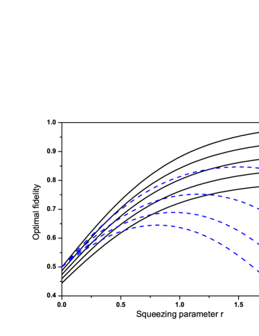
Figure 2: (Colour online) The optimal fidelity for teleporting coherent states as a function of the squeezing parameter $r$ with some different values of $T$ and $\kappa t$ as well as $\bar{n}=0$. Here solid lines: the transmissivity $T=1,0.95,0.9,0.85,0.8$ and $\kappa t=0;$ Blue-dash lines: $\kappa t=0.1,0.2,0.3,0.4$ and $T=1$. The corresponding lines are arranged from top to bottom with the increasing $1/T$ and $\kappa t$, respectively.

In order to examine clearly the effects of different parameters on the optimal fidelity, we plot the optimal fidelities as a function of squeezing parameter $r$ in Fig. 2. From Fig. 2, we can see that for $\kappa t=0$ (without decoherence on mode 3) the optimal fidelities increase monotonically with the increasing squeezing parameter $r$ and the transmissivity $T$. In addition, when we consider the effects of decoherence on mode 3, the optimal fidelities first increase and then decrease with the increasing $r$. The maximal value and the corresponding value of $r_{\max}$ reduces as $\kappa t$ increases. In fact, we can take $\partial\mathcal{F}_{opt}/\partial r=0$ to get a simple relation as following ($\cosh\kappa t=\coth 2r_{\max})$

$$e^{2r_{\max}}=\coth\frac{\kappa t}{2}.$$ (34)

It is interesting to notice that $r_{\max}$ is independent of $T$ and $\bar{n}$.

V Average optimal fidelity and the effect of tunable parameters

In the last section, we consider the $\epsilon$-independent optimal fidelity. However, when $g_{q}\neq 1/(\sqrt{2T}\cos\theta)$ and $g_{p}\neq 1/(\sqrt{2T}\sin\theta)$, the scenario will be changed dramatically. In this case, the fidelity in (24) will depend on the amplitude $\epsilon$ of coherent state. In this section, we examine the average optimal fidelity for three different probability distributions of the teleported input states in which the partial information is known by Alice and Bob. For example, they may be completely sure of phase of the states but the amplitude is unknown 19 .

V.1 Optimal fidelity for teleporting coherent states on a line

First, let us consider the teleportation of coherent states on a line. Without losing the generality, here we assume that the phase of the teleported coherent states is zero because we can always achieve this point by rotating frame. Then the corresponding probability distribution can be given by (letting $\epsilon=x+iy$)

$$P\left(x,y\right)=\frac{1}{2L}\delta\left(y\right)\times\left\{\begin{array}[c]{cc}1,&\left|x\right|\leqslant L\\ 0,&\text{else}\end{array}\right..$$ (35)

Thus substituting Eqs. (35) and (24) into Eq. (21) yields the average fidelity

$$\mathcal{\bar{F}}_{line} =\frac{1}{2L\sqrt{G}}\int_{-L}^{L}dxe^{-\frac{M}{G}x^{2}}$$

$$=\frac{\sqrt{\pi}}{2L\sqrt{M}}\text{Erf}\left\{\frac{|1-\sqrt{2T}g_{q}\cos\theta|}{[H\left(g_{q},\sin\theta\right)]^{1/2}L^{-1}}\right\},$$ (36)

where Erf$\{a\}=$ $1/\sqrt{\pi}\int_{-a}^{a}e^{-x^{2}}dx$ is the error function and $M\left.=\right.(1-\sqrt{2T}g_{q}\cos\theta)^{2}H\left(g_{p},\cos\theta\right)$.

Noticing the separability of $g_{q}$ and $g_{p}$ in $\mathcal{\bar{F}}_{line}$, the optimal value of $g_{p}$ can be obtained by $\partial\mathcal{\bar{F}}_{line}/\partial g_{p}=0$ equivalent to $\partial H\left(g_{p},\cos\theta\right)/\partial g_{p}=0,$ which leads to

$$g_{p}^{opt}=\frac{e^{-\kappa t}\sqrt{2T}\cos\theta^{opt}\sinh 2r}{2(1+2T\cos^{2}\theta^{opt}\sinh^{2}r)}.$$ (37)

It is interesting to notice that the optimal value of $g_{p}^{opt}$ is related to $e^{-\kappa t}$ and $T$ but independent of the average thermal photon-number.

Next, we will maximize the fidelity by numerical calculation. At fixed $r$, $\kappa t$, $\bar{n}$ and $T$, the optimal fidelity of teleportation can be defined as

$$\mathcal{\bar{F}}_{line}^{opt}=\max_{g_{q},g_{p},\theta}\mathcal{\bar{F}}_{line}\left(r,g_{q},g_{p},\theta\right).$$ (38)

In Fig. 3 we plot the optimal fidelity as a function of squeezing parameter $r$ for some different values of parameters $\kappa t$, $\bar{n}$ and $T$. In Fig. 3(a), we consider the optimal fidelities with some different values of $L$ and $T=1,\bar{n}=0$ as well as $\kappa t=0.2$ (for comparison, the case of $\kappa t=0$ is also plotted as dash lines). From Fig. 3(a), we can see that the optimal fidelities grow with increasing $r$ and $1/L$. The fidelities can be greatly optimized with respect to the standard teleportation scheme lines (STS with $g_{q}=g_{p}=1$ and $\theta=\pi/4$, see short dash-dot-(dot) lines). Especially for a smaller $L$ ($L=0.1$), the optimal fidelity can almost access to unit. While for a larger $L$ (say $L=300$), the fidelity achieves a limitation (still over 0.8) which is still superior to that in the STS. In Fig. 3 (b), we consider the effect of different values of $T$ on the optimal fidelity at $\kappa t=0,0.2$. It is shown that the optimal values decease with the increasing $1/T$ for a given $\kappa t$; while for the case of $T\neq 1$, by comparing the fidelities at $\kappa t=0,0.2$ for a given $T$, it is found that the optimal fidelities first increase and then decrease with the increasing $r$, and it is interesting to notice that the optimal fidelity with $\kappa t=0.2$ is superior to that with $\kappa t=0$ when $r$ exceeds a certain cross-point.

Figure 3: The optimal fidelity for teleporting CSs as a function of $r$ with $\bar{n}=0$, $\kappa t=0,0.2$ corresponding to solid and dash lines, respectively. (a) $L=0.1,0.5,1,3,300$ and $T=1;$ for comparison, the teleportation in the STS is also plotted as dash-dot and dash-dot-dot lines for $\kappa t=0,0.2$; (b) $T=1,0.95,0.9,0.85,0.8$ and $L=1$. The corresponding lines are arranged from top to bottom with the increasing $L$ and $1/T$ for a given $\kappa t$.

Furthermore, in order to clearly see whether there is the ability against the decoherence by using these tunable parameters, here we plot the optimied fidelity as a function of the evolution time $\kappa t$ for some fixed values. For this purpose, we fix the squeezing parameter at the intermediate value $r=0.8$ with $T=0.9$, $\bar{n}=0$. Experimentally, the attainable squeezing degree is about $1.5$. Fig. 4 shows that the optimal fidelity remains above 0.8 which exceeds the classical threshold up to significantly large values of $\kappa t$. This case is true even for the limitation of $L\rightarrow\infty$. These results indicate that the optimizal fidelities by three parameters present superior behavior to and higher ability against the decoherence than those in the standard teleportation scheme (with $g_{q}=g_{p}=1$ and $\theta=\pi/4$, also see dash lines in Fig. 4).

Figure 4: (Colour online) The optimal fidelity for teleporting CSs as a function of $\kappa t$ with $\bar{n}=0$, $r=0.8,$ $T=0.9$ and $L=0.1,0.5,1,3,300$ from top to bottom, respectively.

In addition, we make a comparison among the optimal effects of different optimal parameters. In Fig. 5, we plot the optimized fidelity over different tunable parameters as the function of squeezing parameter $r$ for a given $L=1$ with $T=1$, $\bar{n}=0$ and $\kappa t=0.2$. It is found that the optimization by three tunable parameters is the best when compared to single- and two-parameter optimization, especially in the region of small entanglement, which indicates that the role of parameter is different from each other. Thus, it is necessary to perform a simultaneous balanced optimization over these three parameters to obtain a maximization of teleportation fidelity for the probability distribution in Eq. (35).

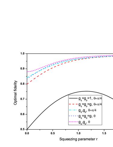
Figure 5: (Colour online) The optimal fidelity for teleporting CSs as a function of $r$ with $\bar{n}=0$, $\kappa t=0.2,$ $T=L=1$ for several different optimal parameters.

V.2 Optimal fidelity for teleporting CSs on a circle

In this subsection, we consider the optimal fidelity for teleporting CSs on a circle, which means $\epsilon=\left|\epsilon\right|e^{i\varphi}\equiv Ae^{i\varphi}$ with a known amplitude $\left|\epsilon\right|=A$ and unknown phase $\varphi$. In this case, the distribution function is $P\left(A,\varphi\right)=\delta\left(\left|\epsilon\right|-A\right)/2\pi$ satisfying $\int_{0}^{\infty}\int_{0}^{2\pi}P\left(A,\varphi\right)d\left|\epsilon\right|d\varphi=1$, then the average fidelity can be calculated as

$$\mathcal{\bar{F}}_{circle}=\frac{e^{-R_{1}}}{\sqrt{G}}\sum_{k=0}^{\infty}\frac{\left(R_{2}\right)^{2k}}{k!k!},$$ (39)

where we have set $R_{1}=A^{2}\{K_{1}[\left(1-f_{1}\right)^{2}+f_{2}^{2}]+4K_{2}\left(1-f_{1}\right)f_{2}\}/G$, $R_{2}=A^{2}\{K_{1}\left(1-f_{1}\right)f_{2}+K_{2}[\left(1-f_{1}\right)^{2}+f_{2}^{2}]\}/G$. Maximizing $\mathcal{\bar{F}}_{circle}$ over these three parameters, we can get the optimized fidelity $\mathcal{\bar{F}}_{circle}^{opt}=\max_{g_{q},g_{p},\theta}\mathcal{\bar{F}}_{circle}\left(r,g_{q},g_{p},\theta\right)$. Our random numerical calculations show that, for the probability distribution, the maximum value of fidelity can be achieved at the point with $g_{q}=g_{p}=g$ and $\theta=\pi/4$, which is different from the case in subsection A. Under this condition we have $f_{1}=f_{3}=g\sqrt{T}$ and $f_{2}=f_{4}=0$, as well as $R_{2}=K_{2}=0$. Thus the optimized fidelity can be given by

$$\mathcal{\bar{F}}_{circle}^{opt}=\frac{1}{\Theta}\exp\left\{-\frac{A^{2}}{\Theta}(1-g\sqrt{T})^{2}\right\},$$ (40)

where we have set $\Theta=\Gamma+[\allowbreak g^{2}(R+1)+1+(g\sqrt{T}-e^{-\kappa t})^{2}\cosh 2r+2g\sqrt{T}e^{-\kappa t}e^{-2r}]/2$. It is obvious that $\Theta>0$.

Using Eq. (39) or (40), we have plotted the optimal fidelity as a function of squeezing parameter $r$ for some different values of $A$ and $T$ in Fig. 6. In Fig. 6(a), we consider the optimal fidelities with some different values of $A$ with $T=1,\bar{n}=0$ as well as $\kappa t=0,0.2$. From Fig. 6(a), we can see that the optimal fidelities grow monotonously with increasing $r$ for $\kappa t=0,$ but for $\kappa t=0.2$ the optimal fidelities first increase and then decrease with increasing $r$ especially for a large $A$ (say $A=3$). In addition, for a small $A$, the optimal fidelity almost access to unit. In Fig. 6(b), we also examine the effect of different $T$ on the fidelity. It is interesting to notice that the optimal fidelity with $\kappa t=0.2$ can be better than that with $\kappa t=0$ when the squeezing $r$ exceeds a certain value. This case is similar to that in Fig. 3(b). In Fig. 6, the point $r_{\max}$ corresponding to the maximum fidelity depends on $\kappa t,$ and for given $\kappa t$, $A$ and $T$, the value of $r_{\max}$ can be determined by taking $\partial\mathcal{\bar{F}}_{circle}^{opt}/\partial r=0,$ which leads to

$$\left\{\Theta-A^{2}(1-g\sqrt{T})^{2}\right\}\frac{\partial\Theta}{\partial r}=0.$$ (41)

After a straightforward calculation, we can abtain

$$\tanh 2r_{\max}=\frac{2g\sqrt{T}e^{-\kappa t}}{g^{2}T+e^{-2\kappa t}}.$$ (42)

or

$$e^{4r_{\max}}-be^{2r_{\max}}+c^{2}=0,$$ (43)

where $b=4[A^{2}(1-g\sqrt{T})^{2}-\Gamma]/(g\sqrt{T}-e^{-\kappa t})^{2},$ and $c=(g\sqrt{T}+e^{-\kappa t})/(g\sqrt{T}-e^{-\kappa t})$. In particular, when $g=1/\sqrt{T}$ the fidelity is independent of the amplitude $A$ and since that $\Theta>0$, the value of $r_{\max}$ in Eq. (42) reduces to that in Eq. (34).

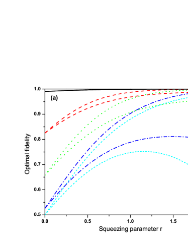
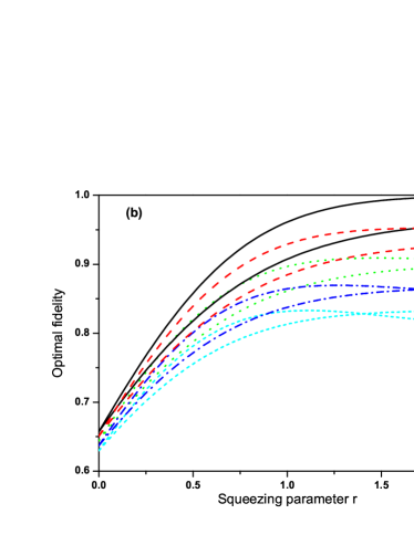
Figure 6: (Colour online) The optimal fidelity for teleporting CSs as a function of $r$ with $\bar{n}=0$, $\kappa t=0,0.2$ (a) $A=0.1,0.5,1,3,300$ and $T=1;$ (b) $T=1,0.95,0.9,0.85,0.8$ and $A=1$. For each optimized case (associated with a special plot style), the corresponding lines are arranged from top to bottom with the increasing $A$ and $1/T$ at the point $r=0$, respectively.

In Fig. 7, choosing the same values of parameters $T,$ $r$ and $\bar{n}$ as in Fig. 4, we plot the optimal fidelity as a function of $\kappa t$. For comparison, we also plot the fidelity without the optimization, i.e., $g_{q}=g_{p}=1$ and $\theta=\pi/4$ (see dash lines). Fig. 7 shows that the teleportation fidelity can be always above the classical limitation 0.5 up to significantly large values of $\kappa t\left(\leqslant 2\right)$ when the amplitude $A$ is less than about $1.7$, and while it can go below the limitation $0.5$ for $A>1.7$ when $\kappa t$ exceeds a certain threshold value. The optimal fidelities with $A=15,300$ are indistinguishable. In the STS, the fidelity is less than 0.5 when $A>15$. Comparing the fidelities with and without optimization, it is shown that the former have better teleportation performance than the latter. However, this improvement is inferior to that shown in Fig. 4 where the optimal fidelities are over 0.8 for any $L$ and $\kappa t$.

Figure 7: (Colour online) The optimal fidelity for teleporting CSs as a function of $\kappa t$ with $\bar{n}=0$, $r=0.8,$ $T=0.9$ and $A=0.1,0.5,1,1.7,3,300$ from top to bottom, respectively.

V.3 Optimal fidelity for teleporting CSs by 2D Gaussian distribution

In the last subsection, we consider another simple probability distribution—–two-dimensional (2D) Gaussian distribution. The corresponding distribution is given by $P\left(\alpha\right)=1/(\pi\chi)\exp[-\left|\alpha\right|^{2}/\chi]$ satisfying $\int P\left(\alpha\right)d^{2}\alpha=1$ 17 ; 19 ; 29 , where the variance parameter $\chi$ determines the cutoff of the amplitude $\alpha$. Thus, using Eqs. (21) and (24), the averaged fidelity can be calculated as

$$\mathcal{\bar{F}}_{G} =\frac{1}{\sqrt{H(g_{p},\cos\theta)+\chi(1-\sqrt{2T}g_{p}\sin\theta)^{2}}}$$

$$\times\frac{1}{\sqrt{H(g_{q},\sin\theta)+\chi(1-\sqrt{2T}g_{q}\cos\theta)^{2}}},$$ (44)

where the function $H(x,y)$ is defined in Eq. (28) [$\left(K_{1}+2K_{2}\right)=H\left(g_{q},\sin\theta\right)$, $\left(K_{1}-2K_{2}\right)=H\left(g_{p},\cos\theta\right)$]. Noticing that the parameters $g_{q}$ and $g_{p}$ are independent from each other in Eq. (44), thus it is not hard to obtain the optimal point by $\partial\mathcal{\bar{F}}_{G}/\partial g_{q}=\partial\mathcal{\bar{F}}_{G}/\partial g_{p}=\partial\mathcal{\bar{F}}_{G}/\partial\theta=0$, i.e., $\theta=\pi/4$ and $g_{q}=g_{p}=g$, where$\ g$ is given by

$$g=\frac{\sqrt{T}\left(e^{-\kappa t}\sinh 2r+2\chi\right)}{2[1+T(\sinh^{2}r+\chi)]}.$$ (45)

At this optimal point, the average optimized fidelity can be expressed as

$$\mathcal{\bar{F}}_{G}^{opt}=\frac{1}{H(g,1/\sqrt{2})+\chi(1-g\sqrt{T})^{2}}.$$ (46)

It is clearly seen that the optimal factor $g$ depends not only on $T$, but also on the evolution time $\kappa t$ in a different form. In particular, when $\allowbreak T\rightarrow 1$ and $\kappa t\rightarrow 0$, Eq. (45) reduces to the result in Ref. 30 . In addition, in the limitation case of $\chi\rightarrow\infty$ which implies that the probability distribution includes the whole complex plane, then we have $g\rightarrow 1/\sqrt{T}$, which just corresponds to the fidelity independent of $\epsilon$.

Using Eq. (44) or (46), we have plotted the optimal fidelity as a function of squeezing parameter $r$ and $\kappa t$ for some different values of $\chi$ in Fig. 8 and Fig. 9, respectively. From Fig. 8, we can see that the smaller the distribution $\chi$ is, the higher the optimal fidelity is. As $\chi$ increases which implies that we have less knowledge of the amplitude of the teleported states, the optimal fidelity approaches to that in the standard scheme ($g=1$). In addition, as $r$ increases, the fidelity first increases up to a $\kappa t$-dependent maximum $r_{\max}$, and then decreases for a larger values of $r$ for a given big $T\chi$. Actually, using $\partial\mathcal{\bar{F}}_{G}^{opt}/\partial r=0$, we can get

$$e^{2r_{\max}}=\frac{\left(e^{\kappa t}+1\right)T\chi+1}{\left(e^{\kappa t}-1\right)T\chi-1}.$$ (47)

For instance, when $T=1,\chi=300$ and $\kappa t=0.2$, then $r_{\max}\simeq 1.\,\allowbreak 16$, which is in agreement with the numerical result in Fig. 8. In Fig. 9, we also consider the effect of decoherence on the fidelity. We can see the similar results to the case of circle distribution. Among these three distributions used above, the line distribution presents the most improvement for fidelity, but the Gaussian distribution presents the lowest improvement. However, a common advantage is that the fidelity with CV can be improved by using the tunable parameters even in the environments when compared with the standard teleportation scheme.

Figure 8: (Colour online) The optimal fidelity for teleporting CSs as a function of $r$ with $\bar{n}=0$, $T=1,$ $\chi=0.1,0.5,1,3,300$ and $T=1.$ For each optimized case (associated with a special plot style), the corresponding lines are arranged from top to bottom with the increasing $\chi$. $\kappa t=0,0.2$ correspond to solid and dash lines, respectively.

Figure 9: (Colour online) The optimal fidelity for teleporting CSs as a function of $\kappa t$ with $\bar{n}=0$, $r=0.8,$ $T=0.9$ and $\chi=0.1,0.5,1,3,300$ from top to bottom, respectively. For comparison, the fidelities with g=1 are plotted here (dash lines).

VI Conclusions

In this paper, we have examined the performance of three-tunable parameters in realistic scheme of CV quantum teleportation with input coherent states and the TMSV entangled resources. For our purpose, we have appealed to the input and output relation in the CF formalism, which is convinent for nonideal inputs and any entangled resources. In this realistic scheme, we have derived the condition that the fidelity is independent of the amplitude of input coherent states for any entangled resource. In order to investigate the effect of three-tunable parameters on the fidelity of teleportation in the nonideal scheme, we have derived the analytical expressions of the optimal fidelity for input coherent states with three different prabability distributions and investigated the performance of optimal fidelity. It is theoretically shown that the usefulness of tunable parameters for improving the fidelity of teleportation with or without the effect of environment and imperfect measurements. In particular, for the input coherent states with a linear distribution, the optimization with three tunable parameters is the best one with respect to single- and two-parameter optimization, especially in the region of small squeezing.

It would be interesting to extend the present analysis to teleport two-mode states (ideal or nonideal cases) using multipartite (non-)Gaussian entangled resources in the formalism of CF. In addition, a recent comparison between the well-known CV VBK scheme and the recently proposed hybrid one by AR has been made 31 ; 32 . It is shown that the VBK teleportation is actually inferior to the AR teleportation within a certain range, even when considering a gain tuning and an optimized non-Gaussian resource. Thus it may be worthy of considering whether these three-parameter optimization can further improve the fidelity in VBK scheme over that in AR scheme especially in the non-ideal scheme.

ACKNOWLEDGEMENTS: This work is supported by a grant from the Qatar National Research Fund (QNRF) under the NPRP project 7-210-1-032. L. Y. Hu is supported by the China Scholarship Council (CSC) and the National Natural Science Foundation of China (No.11264018), as well as the Natural Science Foundation of Jiangxi Province (No. 20151BAB212006).

References

- (1) C. H. Bennett, G. Brassard, C. Crépeau, R. Jozsa, A. Peres, and W. K. Wootters, “Teleporting an unknown quantum state via dual classical and Einstein-Podolsky-Rosen channels,” Phys. Rev. Lett. 70, 1895 (1993).
- (2) L. Vaidman, “Teleportation of quantum states,” Phys. Rev.A 49, 1473 (1994).
- (3) S. L. Braunstein and H. J. Kimble, “Teleportation of Continuous Quantum Variables,” Phys. Rev. Lett. 80, 869 (1998).
- (4) M. S. Zubairy, “Quantum teleportation of a field state,” Phys. Rev. A 58, 4368 (1998).
- (5) A. Ourjoumtsev, A. Dantan, R. Tualle-Brouri, P. Grangier, “Increasing entanglement between Gaussian states by coherent photon subtraction,” Phys. Rev. Lett. 98, 030502 (2007).
- (6) T. Opatrný, G. Kurizki and D.-G. Welsch, “Improvement on teleportation of continuous variables by photon subtraction via conditional measurement,” Phys. Rev. A 61, 032302 (2000).
- (7) P. T. Cochrane, T. C. Ralph and G. J. Milburn, “Teleportation improvement by conditional measurements on the two-mode squeezed vacuum,” Phys. Rev. A 65, 062306 (2002).
- (8) A. Kitagawa, M. Takeoka, M. Sasaki, A. Chefles, “Entanglement evaluation of non-Gaussian states generated by photon subtraction from squeezed states,” Phys. Rev. A 73, 042310 (2006).
- (9) S. Y. Lee, S. W. Ji, C. W. Lee, “Increasing and decreasing entanglement characteristics for continuous variables by a local photon subtraction,” Phys. Rev. A 87, 052321 (2013).
- (10) T. J. Bartley, Philip J. D. Crowley, A. Datta, J. Nunn, L. J. Zhang, I. Walmsley, “Strategies for enhancing quantum entanglement by local photon subtraction,” Phys. Rev. A 87, 022313 (2013).
- (11) J. Fiurasek, “Improving entanglement concentration of Gaussian states by local displacements,” Phys. Rev. A 84, 012335 (2011).
- (12) C. Navarrete-Benlloch, R. Garcia-Patron, J. H. Shapiro, N. J. Cerf, “Enhancing quantum entanglement by photon addition and subtraction,” Phys. Rev. A 86, 012328 (2012).
- (13) S. L. Zhang and P. van Loock “Local Gaussian operations can enhance continuous-variable entanglement distillation,” Phys. Rev. A 84, 062309-1-7 (2011).
- (14) L. Y. Hu, X. X. Xu, and H. Y. Fan, “Statistical properties of photon-subtracted two-mode squeezed vacuum and its decoherence in thermal environment,” J. Opt. Soc. Am. B 27, 286–299 (2010).
- (15) S. Y. Lee and H. Nha, “Quantum state engineering by a coherent superposition of photon subtraction and addition,” Phys. Rev. A 82, 053812-1-7 (2010).
- (16) S. Y. Lee, S. W. Ji, H. J. Kim, and H. Nha, “Enhancing quantum entanglement for continuous variables by a coherent superposition of photon subtraction and addition,” Phys. Rev. A ,84, 012302-1-6 (2011).
- (17) F. Dell’Anno, S. De Siena, L. Albano, and F. Illuminati, “Continuous-variable quantum teleportation with non-Gaussian resources,” Phys. Rev. A 76, 022301 (2007).
- (18) F. Dell’Anno, S. De Siena, and F. Illuminati, “Realistic continuous-variable quantum teleportation with non-Gaussian resources,” Phys. Rev. A 81, 012333 (2010).
- (19) A. Vukics, J. Janszky, and T. Kobayashi, “Nonideal teleportation in coherent-state basis,” Phys. Rev. A 66, 023809 (2002).
- (20) P. T. Cochrane and T. C. Ralph, “Tailoring teleportation to the quantum alphabet,” Phys. Rev. A 67, 022313 (2003).
- (21) A. Furusawa, J. L. Søensen, S. L. Braunstein, C. A. Fuchs, H. J. Kimble, E. S. Polzik, “Unconditional Quantum Teleportation,” Science, 282, 706-709 (1998).
- (22) A. V. Chizhov, L. Knöll, and D.-G. Welsch, “Continuous-variable quantum teleportation through lossy channels,” Phys. Rev. A 65, 022310 (2002).
- (23) S. Takeda, T. Mizuta, M. Fuwa, H. Yonezawa, P. van Loock, and A. Furusawa, “Gain tuning for continuous-variable quantum teleportation of discrete-variable states,” Phys. Rev. A 88, 042327 (2013).
- (24) A. V. Chizhov, “Entanglement fidelity of coherent-state teleportation with asymmetric quantum channel ,” JETP Lett. 80, 711 (2004).
- (25) S. Takeda, M. Fuwa, P. van Loock, and A. Furusawa, “Entanglement Swapping between Discrete and Continuous Variables,” Phys. Rev. Lett. 114, 100501 (2015).
- (26) S. Takeda, T. Mizuta, Maria F, P. van Loock and A. Furusawa, “Deterministic quantum teleportation of photonic quantum bits by a hybrid technique,” Nature, 500, 315 (2013).
- (27) S. Pirandola, J. Eisert, C. Weedbrook, A. Furusawa, S. L. Braunstein, “Advances in Quantum Teleportation,” arXiv: 1505.07831 (Nature Photonics Review)
- (28) P. Marian, T. A. Marian, “Continuous-variable teleportation in the characteristic-function description,” Phys. Rev. A 74, 042306 (2006).
- (29) C. W. Gardiner and P. Zoller, Quantum Noise (Springer Berlin, 2000).
- (30) J. X. Zhang, C. D. Xie, F. L. Li, S. Y. Zhu and M. S. Zubairy, “The state evolution formulation of teleportation for continuous variable,” EPL, 56, 478 (2001).
- (31) S. L. Braunstein, C. A. Fuchs, and H. J. Kimble, “Criteriafor continuous-variable quantum teleportation,” J. Mod. Opt. 47, 267, (2000).
- (32) S. L. Braunstein, C. A. Fuchs, H. J. Kimble, and P. van Loock, “Quantum versus classical domains for teleportation with continuous variables,” Phys. Rev. A 64, 022321 (2001).
- (33) I. Kogias, S. Ragy, and G. Adesso, “Continuous-variable versus hybrid schemes for quantum teleportation of Gaussian states,” PRA, 89, 052324 (2014).
- (34) U. L. Andersen and T. C. Ralph, “High-Fidelity Teleportation of Continuous-Variable Quantum States Using Delocalized Single Photons,” Phys. Rev. Lett. 111, 050504 (2013).