Radially Dependent Large Scale Dynamos in Global Cylindrical Shear Flows and the Local Cartesian Limit

Abstract

For cylindrical differentially rotating plasmas, we study large-scale magnetic field generation from finite amplitude non-axisymmetric perturbations by comparing numerical simulations with quasi-linear analytic theory. When initiated with a vertical magnetic field of either zero or finite net flux, our global cylindrical simulations exhibit the magnetorotational instability (MRI) and large scale dynamo growth of radially alternating mean fields, averaged over height and azimuth. This dynamo growth is explained by our analytic calculations of a non-axisymmetric fluctuation-induced EMF that is sustained by azimuthal shear of the fluctuating fields. The standard “$\Omega$ effect” (shear of the mean field by differential rotation) is unimportant. For the MRI case, we express the large-scale dynamo field as a function of differential rotation. The resulting radially alternating large-scale fields may have implications for angular momentum transport in disks and corona. To connect with previous work on large scale dynamos with local linear shear and identify the minimum conditions needed for large scale field growth, we also solve our equations in local Cartesian coordinates. We find that large scale dynamo growth in a linear shear flow without rotation can be sustained by shear plus non-axisymmetric fluctuations–even if not helical, a seemingly previously unidentified distinction. The linear shear flow dynamo emerges as a more restricted version of our more general new global cylindrical calculations.

1 Introduction

Astrophysical rotators, such as stars, galaxies, and accretion disks, commonly show evidence for contemporaneous presence of disordered turbulence and magnetic fields ordered on spatial or temporal scales larger than those of the fluctuations. Explaining this circumstance has been a long standing challenge. In situ amplification of large-scale magnetic fields via some type of large-scale dynamo is likely but how these dynamos operate and saturate in each context remains an active subject of research (for reviews see (Brandenburg & Subramanian, 2005; Blackman, 2015)). How such fields grow given the presence of fluctuations, what are the best analysis methods, and what minimum ingredients for growth are needed (Vishniac & Brandenburg, 1997; Brandenburg et al., 2008; Yousef & et al., 2008; Heinemann et al., 2011; Herault et al., 2011; Squire & Bhattacharjee, 2015) are topics of active investigation.

Beyond stellar and galactic contexts, evidence for large-scale field growth is seen in magnetically dominated laboratory plasmas (Ji et al., 1995; Cothran et al., 2009), and in local and global simulations (Brandenburg et al., 1995; Ebrahimi et al., 2009; Lesur & Ogilvie, 2010; Davis et al., 2010; Simon et al., 2011; Guan & Gammie, 2011; Sorathia et al., 2012; Suzuki & Inutsuka, 2014) of the magnetorotational instability (MRI) (Velikhov, 1959; Balbus & Hawley, 1991). Large-scale fields in MRI flows have been associated with the sustenance of MRI turbulence(Lesur & Ogilvie, 2008; Davis et al., 2010; Simon et al., 2011) are correlated with the convergence of Maxwell stress (Guan & Gammie, 2011; Nauman & Blackman, 2014), and can influence corona formation (Blackman & Pessah, 2009). For a single MRI mode, large-scale magnetic fields generated via an EMF can cause MRI saturation (Ebrahimi et al., 2009). In short, the large-scale dynamos of MRI-unstable systems are of interest both as phenomena on their own, and because they may be closely connected to angular momentum transport in accretion disks by local and nonlocal Maxwell stresses (Blackman & Nauman, 2015). In addition to numerical simulations, flow-dominated laboratory experiments are also investigating the MRI MHD unstable systems in Taylor-Couette flow geometry (Goodman & Ji, 2002; Rüdiger et al., 2003; Kageyama et al., 2004; Noguchi et al., 2002; Sisan et al., 2004; Stefani et al., 2007).

The electromotive force (EMF) from correlated velocity and magnetic field fluctuations is important to all large scale dynamo theories (Moffatt, 1978). In general, correlated fluctuations in the EMF facilitate large-scale field amplification and the form that this takes for cylindrical MHD shear flows is the focus of the present paper.

As the role of large-scale dynamos and large scale fields for MRI turbulence and angular momentum has become increasingly recognized, there is a need for truly global stratified simulations in the long run to best compare to real astrophysics disks. But choices must always be made both due to limited computational resources and for isolating key physical processes that contribute to the global dynamics. The shearing box model has been the workhorse for simulating MRI turbulence for this purpose– but it is a local model and has limitations associated with boundary conditions, box size and so is a limited model for real astrophysical disks (Regev & Umurhan, 2008; Bodo et al., 2008; Blackman & Nauman, 2015). The cylindrical model used here also has some complementary limitations due to its boundary conditions, but on the other hand provides solutions in a real global domain. Moreover, as unstratified shearing simulations go, the shearing box in itself might be thought of as a more restrictive approximation of a global unstratified cylinder of the sort used here.

In contrast to previous studies of local Cartesian shearing box addressing large scale field growth from nonhelical turbulence and linear shear, (Brandenburg, 2005; Yousef & et al., 2008; Heinemann et al., 2011; Squire & Bhattacharjee, 2015), we focus on the more general large-scale dynamo from the combination of non-axisymmetric perturbations and global differentially rotating flows in a cylinder. We show how the combination of imposed non-axisymmetric fluctuations and differential rotation, or linear shear of the fluctuating field, is sufficient to source the electromotive force and generate a large scale magnetic field in this cylindrical geometry. We present the complete quasilinear form of the EMF and show that it models favorably the results direct numerical simulations (DNS) of the MRI when the magnitude and growth rate of these initial fluctuations in the simulations are used as inputs to the quasi-linear single model analysis. The single mode analysis proves useful in showing explicitly that mode-mode coupling is not essential for growth, and for identifying which terms in the EMF dominate. We also show that these conditions for large scale field growth do not depend on whether the shear profile is favorable or unfavorable to the MRI as long as there is a physically motivated source of fluctuations.

To identify the minimum requirements for large scale growth, to connect with previous work, and to compare with the global cylindrical case, we carry out analogous calculations in local Cartesian coordinates. Comparing cylindrical and local Cartesian models, we find that in each case the fluctuation-induced EMF has separate contributions that depend respectively on 1) non-uniformity of the radially sheared non-axisymmetric perturbations 2) the background differential rotation (cylindrical) or linear shear (Cartesian) 3) the mean angular velocity. These three vertical EMF terms can separately generate a large-scale magnetic field. We discuss them in the context of our numerical simulations and the minimum requirements for large scale field growth. We find that non-axisymmetric fluctuations plus linear shear OR uniform rotation provide the two most minimal combinations needed for large scale field growth in local Cartesian limit.

In Sec. 2, we present evidence of large-scale toroidal fields from global nonlinear MHD DNS of the MRI in a cylindrical setup. We derive the general form of the EMF in the quasilinear approximation in cylindrical geometry in Sec. 3. There we also discuss the role of the EMF in field growth (Sec. 3 .2) and consider an example limiting case where radial gradients of the fluctuations are ignored (Sec. 3.3). We compare the EMF expression from cylindrical analytics with numerical calculations in Sec. 4. We find that the terms with direct dependence on mean differential rotation contribute most to the dynamo seen in the simulations. This is examined for a specific nonaxisymmetric MRI mode and it is shown that a toroidal large-scale field is directly generated through the vertical EMF as the result of the coupling of a small-scale fluctuations with the differential rotation. The traditional “$\Omega$ effect” (i.e. growth of mean toroidal field from mean poloidal field by shear)(Moffatt, 1978; Parker, 1979) is unimportant when the initial mean field is purely vertical. Visualizations of the field lines from our nonlinear MRI simulations of the cylinder are presented in Sec. 5 to highlight why non-axisymmetric perturbations are needed for large scale field growth. In Sec. 6 we repeat the quasilinear analysis in local Cartesian coordinates and derive general forms of the EMF in this geometry. We discuss the associated implications for field growth. By analogy to the specific simplifying example in Sec. 3.3, we discuss the limiting case in which the $x$ gradients of the fluctuations vanish (Sec. 6.2). Finally, in Sec. 7, we emphasize that large-scale fields can also be generated even if the rotation profiles would imply stability to the MRI, as long as there is some external supply of non-axisymmetric fluctuations. We conclude in Sec. 8, and also present a Table summarizing the ingredients needed for dynamo action.

2 Direct numerical simulations in a cylinder

We begin with our results from global DNS MHD simulations of the MRI in cylindrical (r, $\phi$, z) geometry using the DEBS (Schnack et al., 1987; Ebrahimi et al., 2009) initial-value code to solve the nonlinear, viscous and resistive MHD equations

$$\frac{\partial\textbf{A}}{\partial t} = -\textbf{E}=S\textbf{V}\times\textbf{B}-\eta\textbf{J}$$ (1)

$$\rho\frac{\partial\textbf{V}}{\partial t} = -S\rho\textbf{V}.\nabla\textbf{V}+S\textbf{J}\times\textbf{B}+P_{m}\nabla^{2}\textbf{V}-S\frac{\beta_{0}}{2}\nabla P$$ (2)

$$\frac{\partial P}{\partial t} = -S\nabla\cdot(P\textbf{V})-S(\Gamma-1)P\nabla\cdot\textbf{V}$$ (3)

$$\frac{\partial\rho}{\partial t} = -S\nabla\cdot(\rho\textbf{V})$$ (4)

B $$= \nabla\times\textbf{A}$$ (5)

J $$= \nabla\times\textbf{B}$$ (6)

where the variables, $\rho,P,V,B,J,$, and $\Gamma$ are the density, pressure, velocity, magnetic field, current, and ratio of the specific heats, respectively. We use the same normalization (Schnack et al., 1987; Ebrahimi et al., 2009; Ebrahimi & Bhattacharjee, 2014), where time, radius and velocity are normalized to the outer radius a, the resistive diffusion time $\tau_{R}=a^{2}/\mu_{0}\eta$, and the Alfvén velocity $V_{A}=B_{0}/\sqrt{\mu_{0}\rho_{0}}$, respectively. The dimensionless parameters, $S=\tau_{R}V_{A}/a$ and $P_{m}$, are the Lundquist number and the magnetic Prandtl number (the ratio of viscosity to resistivity), respectively. the initial state satisfies the equilibrium force balance condition $\frac{\beta_{0}}{2}\nabla p=\rho V_{\phi}^{2}/r$, where $\beta_{0}\equiv 2\mu_{0}P_{0}/B_{0}^{2}$ is normalized to the axis value, and the initial pressure and density profiles are assumed to be radially uniform and unstratified. Pressure and density are evolved, however, they remain fairly uniform during the computations. A no-slip boundary condition is used for the poloidal flow and flow fluctuations. The inner and outer radial boundaries are perfectly conducting so that the tangential electric field, the normal component of the magnetic field, and the normal component of the velocity vanish. The tangential component of the velocity is the rotational velocity of the wall. The azimuthal ($\phi$) and axial ($z$) boundaries are periodic. We assume a radial pressure gradient balances the centrifugal force in equilibrium, but radial gravity and a radial pressure force are interchangeable for our incompressible, unstratified circumstance. The pressure gradient, rather than gravity, is what balances the centrifugal force in cylindrical laboratory experiments designed to test the MRI (Goodman & Ji (2002)).

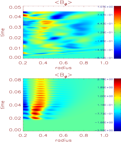
Figure 1: The generation of large-scale toroidal magnetic field (averaged over vertical and toroidal directions) in the zero-net flux simulations in the r-t plane, (a) when all the Fourier modes are included and (b) only one non-axisymmetric mode m=1 is evolved (Rm=3100, Pm=1, $\beta_{0}=10^{5}$, $V_{0}/V_{A}=31$).

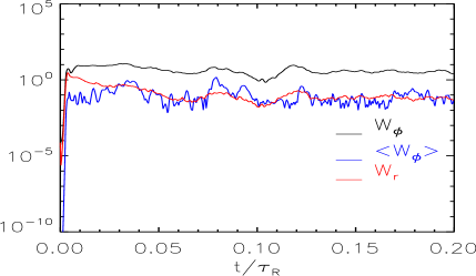
Figure 2: Total magnetic energies, $W_{\phi}=1/2\int{B_{{\phi}}^{2}dr^{3}}$ and $W_{r}=1/2\int{B_{r}^{2}dr^{3}}$, and large-scale toroidal magnetic energy, $\langle W_{\phi}\rangle=1/2\int{\langle B_{{\phi}}\rangle^{2}dr^{3}}$, vs. time for net-zero flux 3-D MRI computations.

All variables are decomposed as $f(r,\phi,z,t)=\sum_{(m,k)}\widehat{f}_{m,k}(r,t)e^{i(-m\phi+kz)}=\langle f(r,t)\rangle+\widetilde{f}(r,\phi\,z,t)$, where $\langle f\rangle$ is the mean $(m=k=0)$ component, and $\widetilde{f}$ is the fluctuating component. Mean quantities (indicated by brackets ($\langle\rangle$) or overbars) are azimuthally and axially averaged, but remain dependent on radius (r). Equations (1-6) are then integrated forward in time using the DEBS code. The DEBS code uses a finite difference method with a staggered grid for radial discretization and pseudospectral method for azimuthal and vertical coordinates. In this decomposition, each mode satisfies a separate equation of the form $\partial\tilde{f}_{m,k}/\partial t=L_{m,k}\tilde{f}_{m,k}+\sum_{(m^{{}^{\prime}},k^{{}^{\prime}})}N_{m,k,m^{{}^{\prime}},k^{{}^{\prime}}}$, where $L_{m,k}$ is a linear operator that depends on $\tilde{f}_{0,0}(r,t)$, and $N_{m,k,m^{{}^{\prime}},k^{{}^{\prime}}}$ is a nonlinear term that represents the coupling of the mode $(m,k)$ to all other modes $(m^{{}^{\prime}},k^{{}^{\prime}})$. ( This latter term is evaluated pseudospectrally.) The time advance is a combination of the leapfrog and semi-implicit methods (Schnack et al., 1987).
We initiate simulations with a Keplerian flow $\langle V_{\phi}(r)\rangle=V_{0}r^{-1/2}$ and uniform magnetic field $\textbf{B}=B_{0}\hat{z}$ (with non-zero initial net-flux) or $\textbf{B}=B_{0}\mathrm{sin}(2\pi(r-r_{1})/(r_{2}-r_{1}))/r\hat{z}$, (with zero-net-flux) where $r_{1}$, $r_{2}$ are the inner and outer radii. Fully nonlinear simulations with all Fourier modes included (with radial, azimuthal and axial resolutions of $n_{r}$=220, $0<m<43$ and $-43<n<43$) show that large-scale magnetic fields are generated [Figure 1(a)]. In all of our simulations, the initially weak vertical magnetic field, gets redistributed, amplified at inner radii and reduced at outer radii. Initially $B_{\phi}$ =0, but a toroidal large-scale (averaged in $\phi$ and $z$) field grows via the correlation of non-axisymmetric MRI-induced fluctuations. The sustenance of total toroidal and radial magnetic field energies, as well as the large-scale toroidal magnetic energy during the computation for net-zero flux are shown in Fig. 2. The radially dependent large-scale field [Figure 1(a)] is also sustained in time.
The code can also be used to compute the nonlinear evolution of a single mode evolution for which the initial conditions consist of an equilibrium $\langle f(r)\rangle$ plus a single mode $\tilde{f}_{m,k}(r,0)\mathrm{e}^{(im\phi+ikz)}$ perturbation. The initial amplitude $\tilde{f}_{m,k}(r,0)$ is a polynomial in $r$ that satisfies the boundary conditions at $r=r_{1}$ and $r=r_{2}$. The initial amplitudes of all other modes are set to zero. Only the mode $(m,k)$ is then evolved; however, the $m=0$, $k=0$ component (the background) is allowed to evolve self-consistently. The evolution of the background profile $\tilde{f}_{0,0}$ can affect the evolution of the mode $(m,k)$ and cause the mode to saturate. In a fully nonlinear computation, all modes are initialized with small random amplitude and are evolved in time, including the full nonlinear term ($N_{m,k,m^{{}^{\prime}},k^{{}^{\prime}}}$).
To facilitate the analytic investigation of the large-scale field generation, we carried out nonlinear single-mode (i.e. single value of $m$ and $k$) simulation of m=1 non-axisymmetric MRI (in which only one fluctuation mode and the mean fields self-consistently grow) for zero-net-flux and net-flux configurations. As seen in Fig. 1(b) at $t\simeq 0.02$, as the m=1 MRI mode amplitude approaches saturation, a large-scale toroidal field is also generated.

3 Quasilinear analytic calculations of EMFs in a cylinder

3.1 Deriving the general form of the EMFs

To identify the origin of large-scale magnetic field growth in the DNS simulations, we employ quasilinear analytical calculations for the single-mode case. Given initial fluctuations we calculate the fluctuation-induced EMF $\overline{\mbox{\boldmath${\cal E}$}}{}\equiv\langle\widetilde{\bf V}\times\widetilde{\bf B}\rangle$ from linearized eigenfunctions. The EMF is the source of large scale field growth. All averaged correlations are presented in terms of the radial Lagrangian displacement $\mathbf{\xi}_{r}$ of a fluid plasma element, (Frieman & Rotenberg, 1960), and the mean quantities. We assume perturbed quantities of the form $\boldsymbol{\xi}(r,\phi,z,t)=[\xi_{r}(r),\xi_{\phi}(r),\xi_{z}(r)]\exp{(\gamma_{c}t-im\phi+ik_{z}z)}$ for a cylinder of outer radius $a$ and height $L=2\pi/k$. In the presence of an equilibrium mean flow, self-adjointness of the linear stability problem is lost (Frieman & Rotenberg, 1960). Thus, for nonaxisymmetric modes (nonzero $m$), the eigenvalues $\gamma_{c}=\gamma+i\omega_{r}$ and the eigenvectors $\xi(r)$ can be complex, where $\gamma$ and $\omega_{r}$ are the growth rate and the oscillation frequency of the mode, respectively. To isolate the role of shear flow on the dynamo effect in the quasilinear analytical calculations below, we impose an initial, uniform $B_{0}$.

For a single MRI Fourier mode, the cylindrical coordinate components of the linearized momentum equation in terms of the Lagrangian displacement vector $\mathbf{\xi}$ (Chandrasekar, 1961) are

$$[\bar{\gamma}^{2}+\omega_{A}^{2}+2r\Omega(r)\Omega^{{}^{\prime}}(r)]\xi_{r}-2\bar{\gamma}\Omega(r)\xi_{\phi}=-\frac{\partial X}{\partial r}$$ (7)

$$(\bar{\gamma}^{2}+\omega_{A}^{2})\xi_{\phi}+2\bar{\gamma}\Omega(r)\xi_{r}=\frac{imX}{r}$$ (8)

$$(\bar{\gamma}^{2}+\omega_{A}^{2})\xi_{z}=-ik_{z}X,$$ (9)

where $\bar{\gamma}=\gamma+i\omega_{r}-im\Omega(r)$, $X=\widetilde{P}+\widetilde{B}\cdot B_{0}$, $\omega_{A}^{2}=k_{z}^{2}B_{0}^{2}/\rho$ and $\Omega(r)=V_{\phi}(r)/r$ is the angular velocity. By including this imposed mean flow in the definition of the Lagrangian displacement vector, the velocity fluctuations in an Eulerian frame are given by $\widetilde{\bf V}=\partial{\boldsymbol{\xi}}/\partial t+\nabla\times(\boldsymbol{\xi}\times\overline{\textbf{V}})$, with components $\widetilde{V}_{r}=\bar{\gamma}\xi_{r}$, $\widetilde{V}_{\phi}=\bar{\gamma}\xi_{\phi}-[\frac{\partial{\overline{V}}_{\phi}}{\partial r}-\frac{{\overline{V}}_{\phi}}{r}]\xi_{r}$ and $\widetilde{V}_{z}=\bar{\gamma}\xi_{z}$.

For small resistivity, the magnetic field perturbations can be directly related to the displacement via $\widetilde{\mathbf{B}}=ik_{z}B_{0}{\boldsymbol{\xi}}$. Using this along with incompressibility and Eqs.( 7-9), we can eliminate $X$ and the azimuthal and vertical displacements can be written in terms of $\xi_{r}$ as

$$\xi_{\phi}=\frac{1}{1+m^{2}/(r^{2}k_{z}^{2})}\left[\frac{-2\Omega(r)\bar{\gamma}}{(\bar{\gamma}^{2}+\omega_{A}^{2})}\xi_{r}-\frac{im}{r^{2}k_{z}^{2}}(r\xi_{r})^{\prime}\right]$$ (10)

and

$$\begin{split}&\xi_{z}=\frac{mk_{z}r}{(r^{2}k_{z}^{2}+m^{2})}\left(\frac{-2\Omega(r)\bar{\gamma}}{\bar{\gamma}^{2}+\omega_{A}^{2}}\right)\xi_{r}\\ &+\frac{i}{rk_{z}}\left(1-\frac{m^{2}}{r^{2}k_{z}^{2}+m^{2}}\right)(r\xi_{r})^{\prime},\end{split}$$ (11)

where the primes indicate radial derivatives. The quasilinear EMF components $\overline{\mbox{${\cal E}$}}{}_{z}=\langle\widetilde{\bf V}\times\widetilde{\bf B}\rangle_{z}={1\over 2}Re(\widetilde{V}_{r}^{*}\widetilde{B}_{\phi}-\widetilde{V}_{\phi}^{*}\widetilde{B}_{r})$ and $\overline{\mbox{${\cal E}$}}{}_{\phi}=\langle\widetilde{\bf V}\times\widetilde{\bf B}\rangle_{\phi}={1\over 2}Re(\widetilde{V}_{z}^{*}\widetilde{B}_{r}-\widetilde{V}_{r}^{*}\widetilde{B}_{z})$ can now be written in terms of the radial velocity fluctuations $\widetilde{V}_{r}=\bar{\gamma}\xi_{r}$,

$$\begin{split}&\overline{\mbox{${\cal E}$}}{}_{Z}=\langle\widetilde{\textbf{V}}\times\widetilde{\textbf{B}}\rangle_{z}=\overline{\mbox{${\cal E}$}}{}_{ZVr^{\prime}}+\overline{\mbox{${\cal E}$}}{}_{Z\Omega^{\prime}}+\overline{\mbox{${\cal E}$}}{}_{Z\Omega},\end{split}$$ (12)

where

$$\overline{\mbox{${\cal E}$}}{}_{ZVr^{\prime}}=\frac{m\gamma k_{z}B_{0}}{(m^{2}+k_{z}^{2}r^{2})}\left[\frac{r\widetilde{V_{r}}\widetilde{V_{r}^{*}}^{\prime}}{\gamma^{2}+\overline{\Omega}^{2}(r)}\right].$$ (13)

$$\overline{\mbox{${\cal E}$}}{}_{Z\Omega^{\prime}}=-\frac{m^{2}\gamma k_{z}B_{0}}{(m^{2}+k_{z}^{2}r^{2})}\left[\frac{\Omega^{\prime}(r)\overline{\Omega}(r)r|\widetilde{V_{r}}|^{2}}{(\gamma^{2}+\overline{\Omega}^{2}(r))^{2}}\right],$$ (14)

$$\begin{split}&\overline{\mbox{${\cal E}$}}{}_{Z\Omega}=\frac{2\gamma k_{z}^{3}B_{0}\Omega(r)r^{2}\overline{\Omega}}{G^{2}}(\gamma^{2}+\overline{\Omega}^{2}-\omega_{A}^{2})|\widetilde{V_{r}}|^{2}\\ &+\frac{m\gamma k_{z}B_{0}}{(m^{2}+k_{z}^{2}r^{2})}\left[\frac{|\widetilde{V_{r}}|^{2}}{\gamma^{2}+\overline{\Omega}^{2}(r)}\right],\end{split}$$ (15)

and

$$\begin{split}&\overline{\mbox{${\cal E}$}}{}_{\phi}=\langle\widetilde{\textbf{V}}\times\widetilde{\textbf{B}}\rangle_{\phi}=\overline{\mbox{${\cal E}$}}{}_{\phi Vr^{\prime}}+\overline{\mbox{${\cal E}$}}{}_{\phi\Omega^{\prime}}+\overline{\mbox{${\cal E}$}}{}_{\phi\Omega},\end{split}$$ (16)

where

$$\overline{\mbox{${\cal E}$}}{}_{\phi Vr^{\prime}}=\left[\frac{\gamma B_{0}}{r}-\frac{m^{2}\gamma B_{0}}{r(m^{2}+k_{z}^{2}r^{2})}\right]\left[\frac{(r\widetilde{V_{r}}\widetilde{V_{r}^{*}}^{\prime})}{\gamma^{2}+\overline{\Omega}^{2}(r)}\right],$$ (17)

$$\overline{\mbox{${\cal E}$}}{}_{\phi\Omega^{\prime}}=-\left[\frac{\gamma B_{0}}{r}-\frac{m^{2}\gamma B_{0}}{r(m^{2}+k_{z}^{2}r^{2})}\right]\left[\frac{\Omega^{\prime}(r)\overline{\Omega}(r)r|\widetilde{V_{r}}|^{2}}{(\gamma^{2}+\overline{\Omega}^{2}(r))^{2}}\right],$$ (18)

$$\begin{split}&\overline{\mbox{${\cal E}$}}{}_{\phi\Omega}=\frac{2\gamma k_{z}^{2}rB_{0}\overline{\Omega}m\Omega(r)}{G^{2}}(\omega_{A}^{2}-\gamma^{2}-\overline{\Omega}^{2})|\widetilde{V_{r}}|^{2}\\ &+\left[\frac{\gamma B_{0}}{r}-\frac{m^{2}\gamma B_{0}}{r(m^{2}+k_{z}^{2}r^{2})}\right]\left[\frac{|\widetilde{V_{r}}|^{2}}{\gamma^{2}+\overline{\Omega}^{2}(r)}\right],\end{split}$$ (19)

where

$$G^{2}=(m^{2}+k_{z}^{2}r^{2})[\gamma^{2}+\overline{\Omega}^{2}(r)][4\gamma^{2}\overline{\Omega}^{2}(r)+(\gamma^{2}+\overline{\Omega}^{2}(r)+\omega_{A}^{2})^{2}]$$ (20)

and $\overline{\Omega}(r)=m\Omega(r)-\omega_{r}$. In an ideal MHD cylindrical plasma, Eq.  (12) provides the complete quasilinear form of the vertical fluctuation-induced EMF in terms of radial perturbations. The first term on the RHS, $\overline{\mbox{${\cal E}$}}{}_{ZVr^{\prime}}$, depends on the non-uniformity of the radial displacement of the mode. The second term $\overline{\mbox{${\cal E}$}}{}_{Z\Omega^{\prime}}$, which depends on the differential rotation $\Omega^{\prime}(r)$ is sufficient to directly produce a nonzero fluctuation-induced dynamo term. The free energy source $\frac{d\Omega^{2}}{dlnr}$ appears in this term. The third term, $\overline{\mbox{${\cal E}$}}{}_{Z\Omega}$, shows the dependence of the vertical EMF on angular velocity.

The linearized cylindrical solutions ($\gamma$ and $\xi_{r}$) for nonaxisymmetric flow-driven and MRI modes have been previously examined (Bondeson et al., 1987; Ogilvie & Pringle, 1996; Keppens et al., 2002). Here we do not solve the eigenvalue problem to find the $\xi_{r}$ for nonaxisymmetric modes but (in Sec. 4,) extract the linearized solutions directly from DNS for a single mode and verify the quasilinear forms of EMFs.

The above quasilinear EMF terms allow us to identify the source of large scale magnetic field growth in a rotating plasma with or without radially sheared non-axisymmetric perturbations.

3.2 EMFs and Large Scale Field Growth

The dominance of the fluctuation-induced quasilinear $\overline{\mbox{${\cal E}$}}{}_{Z}$ in the generation of the large-scale toroidal magnetic field can be seen by examining the mean (averaged in $\phi$ and $z$) toroidal component of the induction equation, ignoring resistivity. This equation is

$$\frac{\partial\overline{\textbf{B}_{\phi}}}{\partial t}=-\frac{\partial\overline{\mbox{${\cal E}$}}{}_{z}}{\partial r}+(\overline{\textbf{B}}\cdot\nabla)\overline{\textbf{V}}|_{\phi}-(\overline{\textbf{V}}\cdot\nabla)\overline{\textbf{B}}|_{\phi}.$$ (21)

Since there is neither a mean radial magnetic field ${\overline{B}}_{r}$, nor velocity field ${\overline{V}}_{r}$, so the second and third terms on the right of Eq. (21) vanish. Note that the second term on the right of Eq. (21) is the traditional ”$\Omega$ effect” which thus vanishes for our setup and averaging procedure. The shear (differential rotation) does enter through $\overline{\mbox{${\cal E}$}}{}_{z}$, and the first term on the right of Eq. (21) is the dominant term.

Keeping only the first term on the right of Eq. (21) ($\frac{\partial\overline{\textbf{B}_{\phi}}}{\partial t}=-\frac{\partial\overline{\mbox{${\cal E}$}}{}_{z}}{\partial r}$) we then see that the three terms on the right of Eq.  (12) provide distinct paths for large scale fields to grow: (1) Radially sheared non-axisymmetric perturbations i. e., the first term in Eq.  (12), $\overline{\mbox{${\cal E}$}}{}_{ZVr^{\prime}}$, proportional to the non-uniformity of the radial displacement of the nonaxisymmetric perturbation (2) Uniform non-axisymmetric perturbations (stable or unstable) but with background shear in the angular flow i. e. the last two terms in Eq.  (12). We emphasize that all three terms on the right of $\overline{\mbox{${\cal E}$}}{}_{Z}$ (Eq.  12) vanish explicitly for axisymmetric modes (m=0 modes, $\overline{\Omega}=0$), as axisymmetric modes are purely growing or decaying (i.e. $\omega_{r}=0$) (Chandrasekar, 1961).

The induction equation for the vertical mean field is

$$\frac{\partial\overline{\textbf{B}_{z}}}{\partial t}=\frac{\partial\overline{\mbox{${\cal E}$}}{}_{\phi}}{\partial r}+(\overline{\textbf{B}}\cdot\nabla)\overline{\textbf{V}}|_{z}-(\overline{\textbf{V}}\cdot\nabla)\overline{\textbf{B}}|_{z}.$$ (22)

Here again, as in equation (21), the last two terms on the right vanish and the mean field evolves only through the EMF term $\partial\overline{\mbox{${\cal E}$}}{}_{\phi}/dr$. For this equation, axisymmetric modes can contribute through the radial variations of $\widetilde{V}_{r}$ in $\overline{\mbox{${\cal E}$}}{}_{\phi Vr^{\prime}}$ (Eq. 16) and the last term in Eq. (19) to give

$$\overline{\mbox{${\cal E}$}}{}_{\phi(m=0)}=\left(\frac{B_{0}}{\gamma}\right)[\widetilde{V_{r}}\widetilde{V_{r}^{*}}^{\prime}+|\widetilde{V_{r}}|^{2}/r],\\ \overline{\mbox{${\cal E}$}}{}_{Z(m=0)}=0$$ (23)

but only non-axisymmetric modes allow evolution of both ${\overline{B}}_{z}$ and ${\overline{B}}_{\phi}$ through the EMF terms.

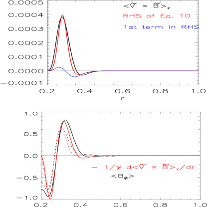
Figure 3: The profiles of (a) (in black) direct numerical calculations of total vertical EMF term, LHS of Eq. (12); (in red) RHS side of Eq. (12) based on the quasilinear calculations; (in blue) the first term in Eq. (12). Linear growth rate of the mode at the early phase $\gamma\tau_{orbit}\sim 0.9$ and $\omega_{r}\tau_{orbit}\sim 2.2$ have been used for the calculations of RHS, (b) $\langle B_{\phi}\rangle$ and $-{1\over\gamma}\frac{\partial\overline{\mbox{${\cal E}$}}{}_{z}}{\partial r}$ at $t/\tau_{orbit}=16$ and $t/\tau_{orbit}=10$ during the growth of m=1 MRI mode from DNS with non-zero net flux (solid lines) and zero net flux (dashed lines), respectively. The dimensionless magnetic and velocity fluctuations at this time of DNS are $|\widetilde{B_{\phi}}/B_{0}|\sim 0.06$ and $|\widetilde{B_{r}}/B_{0}|={k_{z}a|\widetilde{V_{r}}/V_{A}|\over k_{0}\gamma\tau_{A}}\sim 0.015$, and using DNS values of $\gamma\tau_{A}\sim 12$, $|\widetilde{V_{r}}/V_{A}|\sim 0.015$, ($V_{0}/V_{A}=16$).

3.3 EMFs appropriate for MRI driven fluctuations when $k_{r}=0$

To simplify pinpointing the dominant contributions to the EMF from the quasi-linear theory appropriate for MRI driven fluctuations for an initially vertical field, we assume $\widetilde{V_{r}^{\prime}}=0$ (in the limit of $k_{r}=0$). This is justified since Fig. 3(a) from DNS in the following section shows that the term arising from this radial gradient is subdominant. We can now solve the quasilinear equations for $\overline{\mbox{${\cal E}$}}{}_{z}$ without knowing the exact form of the global eigenfunctions. For large growth rates (i.e. $\gamma^{2},{\overline{\Omega}}^{2}>\omega_{A}^{2}$), Eq. (12) then reduces to

$$\begin{split}&\overline{\mbox{${\cal E}$}}{}_{Z}(r)\sim\frac{\gamma kB_{0}}{(m^{2}+k^{2}r^{2})}\left[m-\frac{m^{2}\Omega^{\prime}(r)\overline{\Omega}(r)r}{\gamma^{2}+\overline{\Omega}^{2}}+\frac{2k^{2}{V}_{\phi}r\overline{\Omega}}{\gamma^{2}+\overline{\Omega}^{2}}\right]\\ &\times(\frac{|\widetilde{V_{r}}|^{2}}{\gamma^{2}+\overline{\Omega}^{2}(r)}).\end{split}$$ (24)

This vertical EMF for a single nonaxisymmetic mode and the mean flow (e.g. Keplerian) with $\gamma\sim\Omega_{0}$ (where $\Omega_{0}$ is the angular frequency at the inner radial boundary) in the $k_{z}r>m$ and $\gamma^{2}>{\overline{\Omega}}^{2}$ limits are then related by $\overline{\mbox{${\cal E}$}}{}_{z}\sim-\frac{m^{2}B_{0}}{k_{z}r^{2}\gamma^{3}}\frac{d\Omega(r)^{2}}{dlnr}|\widetilde{V_{r}}|^{2}+2mkB_{0}\frac{\Omega(r)\overline{\Omega}(r)}{\gamma^{3}}|\widetilde{V_{r}}|^{2}\equiv Q(r)\widetilde{V_{r}}|^{2}.$ Using this equation and $\overline{B}_{\phi}\sim-{1\over\gamma}\frac{\partial\overline{\mbox{${\cal E}$}}{}_{z}}{\partial r}$ in the limit of constant $\widetilde{V}_{r}$ and constant mean vertical magnetic field $B_{0}$, the large-scale toroidal magnetic field can be written as

$${\overline{B}}_{\phi}(r)\sim-\frac{m^{2}B_{0}}{k_{z}\gamma^{4}}\left[\frac{1}{r^{2}}\frac{d\Omega(r)^{2}}{dlnr}\right]^{\prime}|\widetilde{V_{r}}|^{2}+\frac{2mkB_{0}}{\gamma^{4}}\left[\Omega(r)\overline{\Omega}(r)\right]^{\prime}|\widetilde{V_{r}}|^{2},$$ (25)

showing a direct relationship between differential rotation and the generation of large-scale magnetic field.

4 Comparing theory with DNS of a nonaxisymmetric mode

From DNS of a nonaxisymmetric mode $m=1$, $k_{z}a$=12 in cylindrical model (Sec. 2), we evaluate $\langle\widetilde{\textbf{V}}\times\widetilde{\textbf{B}}\rangle_{z}$ and compare it to quasilinear calculations of the right side (RHS) of Eq. (12) in terms of radial velocity fluctuations $\widetilde{V}_{r}=\bar{\gamma}\xi_{r}$. For the RHS of Eq. (12), the radial velocity fluctuations and the eigenvalues from DNS are inserted into the analytical forms. Fig. 3(a) shows good agreement between these two calculations. Fig. 3(a) also shows that the first term on the RHS of Eq. (12) is subdominant to the last two terms which depend on the mean flow.

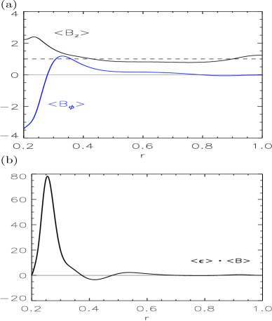
Figure 4: Radial profiles of time-averaged (b) saturated large-scale fields $\langle B_{z}\rangle,\langle B_{\phi}\rangle$, (b) $\overline{\mbox{${\cal E}$}}{}\cdot\overline{\bf B}$ ( = S $\langle\widetilde{\textbf{V}}\times\widetilde{\textbf{B}}\rangle$ $\cdot\langle\textbf{B}\rangle$ from DNS of Eq. (1-6) during nonlinear evolution of m=1 MRI.

We have verified the dominance of the first term on the right of Eq. (21) from DNS of a single-mode m=1 MRI. The large-scale ${\overline{B}}_{\phi}$ starts to grow, even when initially zero, as the instability develops. Figure 3(b) shows $\langle B_{\phi}\rangle$ as computed from the DNS during the linear phase of single-mode simulations with non-zero net flux and the first term on the RHS of Eq. (21), right before the saturation, as also measured from the DNS. As seen, the mean toroidal field is correlated with, and directly generated by the vertical EMF. Similarly, the mean $B_{\phi}$ generated in the net-zero flux simulations shown in Fig. 1 is also correlated with the vertical EMF. Fig 3(a) shows that the main contribution to the EMF comes from the last two terms of Eq. (12). Thus $B_{\phi}\sim-{1\over\gamma}\frac{\partial\langle(\widetilde{\textbf{V}}\times\widetilde{\textbf{B}})_{z}\rangle}{\partial r}$ is directly dependent on the shear-flow ($V_{\phi}^{\prime}$) or differential rotation ($d\Omega/dr$) in the presence of a finite amplitude fluctuation.

In addition to the EMF components themselves, the magnetic field-aligned EMF plays important role in the quasi-linear regime as the mode starts to saturate. Evolution of both components (toroidal and vertical) of the large-scale magnetic field is only possible for nonaxisymmetric fluctuations because only in this case are both $\overline{\mbox{${\cal E}$}}{}_{z}$ and $\overline{\mbox{${\cal E}$}}{}_{\phi}$ (Eq. 12, 16) non-zero. The generation of the large-scale toroidal field is due to the vertical EMF and the redistribution (and amplification around r=0.2-0.4) of ${\overline{B}}_{z}$ is due to the nonzero toroidal EMF. Figure 4 shows the profiles of time-averaged saturated large-scale toroidal and vertical fields as well as the EMF parallel to $\overline{\bf B}$.

Simulations with axisymmetric fluctuations also show the amplification of vertical large-scale field ($B_{z}$) but without a generation of $B_{\phi}$. The amplification of $B_{z}$ from axisymmetric modes (Eq. 23), which may contribute to the mode saturation in a cylinder (Ebrahimi et al., 2009) results from the curvature terms and is absent for channel modes in a local Cartesian model, as discussed below.

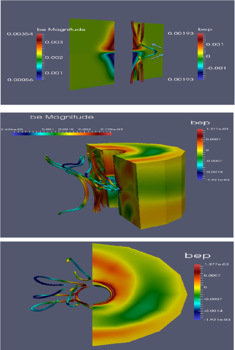
Figure 5: Field line visualizations during nonlinear MRI simulations in a cylinder (a) 2-D (b) 3-D when m=1 mode perturbation is dominant (c) toroidal top view in 3-D shows the twisting of the field lines.

5 Visualizations from Numerical Simulations

The physical picture of generating $\langle B_{\phi}\rangle$ can further be examined through comparing visualizations of the field lines without and with nonaxisymmetric MRI perturbations in 2-D and 3-D as shown in Fig. 5. For toroidal m=0 perturbations, weak vertical magnetic field lines are toroidally stretched (Fig. 5(a)) according to the second term in Eq. (21). However due to toroidal symmetry, $\langle B_{\phi}\rangle=0$ as the positive and negative contributions from the perturbations remain on the same vertical surface, and only the mean vertical field is amplified through $\partial\overline{\mbox{${\cal E}$}}{}_{\phi}/dr$. (Ebrahimi et al., 2009). In the presence of nonaxisymmetric perturbations in 3-D nonlinear simulations however, the field lines are stretched and twisted (Fig. 5 b,c). As a consequence, $\langle B_{\phi}\rangle\neq 0$ since now the oppositely signed toroidal field contributions from perturbations are displaced radially from one another. Since $\langle B_{r}\rangle$ is zero, the standard “$\Omega$ effect” [$\langle B_{r}\rangle V_{\phi}^{\prime}$] contribution in Eq. (21) is zero.

6 Local Cartesian Quasilinear analytic calculations of EMFs

6.1 General form of the EMFs

Here, we present the analog to Eqs. (7-12) in local Cartesian coordinates $(x,y,z)$ in a frame rotating with fixed angular velocity $\mathbf{\Omega}=\Omega_{0}\textbf{e}_{z}$ and a linear shear velocity of $\textbf{V}_{0}=V_{y}(x)\textbf{e}_{y}$. We again assume a vertical field $B_{0}{\hat{\bf}z}$ but now assume perturbed velocity and magnetic field of the form $\boldsymbol{\xi}(x,y,z,t)=[\xi_{x}(x),\xi_{y}(x),\xi_{z}(x)]\exp{(\gamma_{c}t-ik_{y}y+ik_{z}z)}$, where, $\gamma_{c}=\gamma+i\omega_{r}$. In this rotating unstratified system, we include the Coriolis force and the centrifugal force, and again assume that in equilibrium, the latter is canceled by the radial pressure gradient. (As for the cylindrical case, the role of gravity vs. radial pressure gradient are interchangeable for our incompressible, unstratified case. ) The momentum equation $\rho\frac{\partial\textbf{V}}{\partial t}=-\rho\textbf{V}.\nabla\textbf{V}+2(\mathbf{\Omega}\times\textbf{V})+\mathbf{\Omega}\times\mathbf{\Omega}\times{\bf r}+\textbf{J}\times\textbf{B}-\nabla P$ and the induction equation $\partial_{t}{\bf B}=\nabla\times({\bf V}\times{\bf B})$ are linearized in the incompressible limit to give:

$$\begin{split}\bar{\gamma}\widetilde{V}_{x}-2\Omega_{0}\widetilde{V}_{y}&=ik_{z}B_{0}\widetilde{B}_{x}/\rho-\frac{\partial X}{\partial x}\\ \bar{\gamma}\widetilde{V}_{y}+V_{y}^{\prime}(x)\widetilde{V}_{x}+2\Omega_{0}\widetilde{V}_{x}&=ik_{z}B_{0}\widetilde{B}_{y}/\rho+ik_{y}X\\ \bar{\gamma}\widetilde{V}_{z}&=ik_{z}B_{0}\widetilde{B}_{z}/\rho-ik_{z}X\end{split}$$ (26)

and

$$\begin{split}\bar{\gamma}\widetilde{B}_{x}&=ik_{z}B_{0}\widetilde{V}_{x}\\ \bar{\gamma}\widetilde{B}_{y}&=V_{y}(x)^{\prime}\widetilde{B}_{x}+ik_{z}B_{0}\widetilde{V}_{y}\\ \bar{\gamma}\widetilde{B}_{z}&=ik_{z}B_{0}\widetilde{V}_{z},\end{split}$$ (27)

where primes denote variation in x direction, ($e.g.\ \partial/\partial x$) Using $\widetilde{V}_{x}=\bar{\gamma}\xi_{x}$, $\widetilde{V}_{y}=\bar{\gamma}\xi_{y}-V_{y}^{{}^{\prime}}(x)\xi_{x}$ and $\widetilde{V}_{z}=\bar{\gamma}\xi_{z}$, Eqs. (26) and (27) can be written in terms of the displacement vector as

$$[\bar{\gamma}^{2}+\omega_{A}^{2}+2r\Omega_{0}V_{y}^{{}^{\prime}}(x)]\xi_{x}-2\bar{\gamma}\Omega_{0}\xi_{y}=-\frac{\partial X}{\partial x}$$ (28)

$$(\bar{\gamma}^{2}+\omega_{A}^{2})\xi_{y}+2\bar{\gamma}\Omega_{0}\xi_{x}=ik_{y}X$$ (29)

$$(\bar{\gamma}^{2}+\omega_{A}^{2})\xi_{z}=-ik_{z}X.$$ (30)

Analogous to the cylindrical case (Sec. 3), from these sets of equations, the quasilinear vertical EMF in terms of the Eulerian velocity fluctuations ($\widetilde{\bf V}=\partial{\boldsymbol{\xi}}/\partial t+\overline{\textbf{V}}\cdot\nabla{\boldsymbol{\xi}}-{\boldsymbol{\xi}}\cdot\nabla\overline{\textbf{V}}$), $\widetilde{V}_{x}=\bar{\gamma}\xi_{x}$ is reduced to:

$$\begin{split}&\overline{\mbox{${\cal E}$}}{}_{z}=\langle\widetilde{\textbf{V}}\times\widetilde{\textbf{B}}\rangle_{z}=\overline{\mbox{${\cal E}$}}{}_{ZVr^{\prime}}+\overline{\mbox{${\cal E}$}}{}_{Z(shear)}+\overline{\mbox{${\cal E}$}}{}_{Z\Omega},\end{split}$$ (31)

where

$$\overline{\mbox{${\cal E}$}}{}_{ZVx^{\prime}}=\frac{k_{y}\gamma k_{z}B_{0}}{(k_{y}^{2}+k_{z}^{2})}\left[\frac{\widetilde{V_{x}}\widetilde{V_{x}^{*}}^{\prime}}{\gamma^{2}+\vartheta^{2}(x)}\right],$$ (32)

$$\overline{\mbox{${\cal E}$}}{}_{Z(shear)}=-\frac{k_{y}\gamma k_{z}B_{0}}{(k_{y}^{2}+k_{z}^{2})}\left[\frac{k_{y}V_{y}(x)^{\prime}(k_{y}V_{y}(x)-\omega_{r})}{(\gamma^{2}+\vartheta^{2}(x))^{2}}\right]|\widetilde{V_{x}}|^{2},$$ (33)

and

$$\begin{split}&\overline{\mbox{${\cal E}$}}{}_{Z\Omega 0}=\frac{2\gamma k_{z}^{3}B_{0}\Omega_{0}\vartheta(x)}{G^{2}}(\gamma^{2}+{\vartheta(x)}^{2}-\omega_{A}^{2})|\widetilde{V_{x}}|^{2},\end{split}$$ (34)

where $\vartheta(x)=k_{y}V_{y}(x)-\omega_{r}$, $\bar{\gamma}=\gamma-i\vartheta(x)$, and $G^{2}=(k_{y}^{2}+k_{z}^{2})(\gamma^{2}+\vartheta^{2}(x))[4\gamma^{2}\vartheta^{2}(x)+(\gamma^{2}+\vartheta^{2}(x)+\omega_{A}^{2})^{2}]$. As seen in these equations, in the local Cartesian model, the rotation and shear are independent.

The first contribution $\overline{\mbox{${\cal E}$}}{}_{ZVx^{\prime}}$ shows how nonaxisymmetric perturbations with radial shear, even without any explicit mean shear flow can source a vertical EMF. In the absence of rotation, the second contribution, $\overline{\mbox{${\cal E}$}}{}_{Z(shear)}$, shows a direct dependence of vertical EMF on the linear shear. A mean shear flow, $V_{y}(x)^{\prime}$ combined with a radially uniform non-axisymmertic ($k_{y}\neq 0$) perturbation is sufficient to produce $\overline{\mbox{${\cal E}$}}{}_{Z(shear)}$. The last contribution $\overline{\mbox{${\cal E}$}}{}_{Z\Omega}$, which vanishes in the absence of angular velocity, shows that a contribution to the vertical EMF can result from a finite angular velocity ($\Omega_{0}$) for non-axisymmetric perturbations.

Similarly the azimuthal EMF is given by

$$\begin{split}&\overline{\mbox{${\cal E}$}}{}_{y}=\langle\widetilde{\textbf{V}}\times\widetilde{\textbf{B}}\rangle_{y}=\overline{\mbox{${\cal E}$}}{}_{yVr^{\prime}}+\overline{\mbox{${\cal E}$}}{}_{y(shear)}+\overline{\mbox{${\cal E}$}}{}_{y\Omega_{0}},\end{split}$$ (35)

where

$$\overline{\mbox{${\cal E}$}}{}_{yVx^{\prime}}=\gamma B_{0}\left[1-\frac{k_{y}^{2}}{(k_{y}^{2}+k_{z}^{2})}\right]\left[\frac{(\widetilde{V_{x}}\widetilde{V_{x}^{*}}^{\prime})}{(\gamma^{2}+\vartheta^{2}(x))}\right],$$ (36)

$$\overline{\mbox{${\cal E}$}}{}_{y(shear)}=-\gamma B_{0}\left[1-\frac{k_{y}^{2}}{(k_{y}^{2}+k_{z}^{2})}\right]\left[\frac{k_{y}V_{y}(x)^{\prime}(k_{y}V_{y}(x)-\omega_{r})|\widetilde{V_{x}}|^{2}}{(\gamma^{2}+\vartheta^{2}(x))^{2}}\right],$$ (37)

and

$$\begin{split}&\overline{\mbox{${\cal E}$}}{}_{y\Omega 0}=\frac{2\gamma k_{z}^{2}B_{0}\Omega_{0}k_{y}(k_{y}V_{y}(x)-\omega_{r})}{G^{2}}(\omega_{A}^{2}-\gamma^{2}-\vartheta^{2}(x))|\widetilde{V_{x}}|^{2}.\end{split}$$ (38)

Spatial derivatives of Eq. (35) could, in principle, also generate and redistribute the vertical field $B_{z}$ due to nonaxisymmetric modes ($k_{y}\neq 0$). However, the fastest growing axisymmetric modes–the channel modes ($k_{y}=k_{x}=0$)—do NOT contribute in either the vertical or azimuthal EMF (Eq. 31 and Eq. 35) obtained above. In contrast, for the global cylindrical model, even for radially uniform axisymmetric modes ($k_{r}=m=0$), the last term in Eq. (23) DOES contribute in the amplification of vertical field. This distinction highlights at least one circumstance in which the absence of curvature in the Cartesian model removes a contribution that could be present in the global rotator.

6.2 Exact expression for large scale field with only linear shear when $k_{x}=0$

A large-scale magnetic field can be generated by the EMF of Eq. (31) from any of the independent contributions in  (32- 34). In the absence of rotation, a large-scale magnetic field, $\overline{B}_{y}\sim-{1\over\gamma}\frac{\partial\overline{\mbox{${\cal E}$}}{}_{z}}{\partial x}$, can directly be generated via a linear flow-shear and a radially uniform non-axisymmetric ($k_{y},k_{z}\neq 0$, $k_{x}=0$) perturbation,

$${\overline{B}}_{y}(x)=\frac{k_{y}k_{z}B_{0}}{(k_{y}^{2}+k_{z}^{2})}\left[\frac{k_{y}V_{y}(x)^{\prime}(k_{y}V_{y}(x)-\omega_{r})}{(\gamma^{2}+\vartheta^{2}(x))^{2}}\right]^{\prime}|\widetilde{V_{x}}|^{2},$$ (39)

This is an exact analytical equation for a large-scale azimuthal magnetic field generated via a linear mean shear-flow and any perturbations with nonzero $k_{y}$ and $k_{z}$.

The large-scale field given in Eq. (39) is consistent with previous studies of large scale field growth from the combination of linear shear with randomly forced turbulence (Vishniac & Brandenburg, 1997; Yousef & et al., 2008; Heinemann et al., 2011; Mitra & Brandenburg, 2012; Sridhar & Singh, 2014). However, our calculations explicitly reveal the most minimalist conditions needed for growth in the absence of rotation: a background linear shear and an imposed non-axisymmetric perturbation with nonzero $k_{y},k_{z}$. Helical velocity perturbations are not required.

Generation of ${\overline{B}}_{y}$ in this case of mean shear can be visualized by considering an perturbation in the $x$ direction and then considering why both $z$ and $y$ variations are needed to produce a net field in vertically averaged planes. If there were no $z$ variation in the perturbation then the mean shear would produce no toroidal field even before vertically averaging. And if there were a vertical variation but no $y$ variation, then the the mean shear would produce ${\overline{B}}_{y}(x)=0$ from vertical averaging.

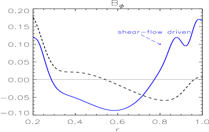
Figure 6: $B_{\phi}$ generated with positive shear flow ($V_{\phi}(r)/V_{A}=80(r/a)^{3}$) and large initial amplitude forcing (solid line); and only with forcing amplitude varying with radius (dashed line).

7 Large-scale field in the case of stable flow

Our quasi-linear theory imposes fluctuations and background shear as a starting point whereas in DNS, the fluctuations can directly result from the MRI. The quasilinear theory shows that the growth of $\overline{B}_{\phi}$ in Eq. (21) via $\partial_{r}\overline{\mbox{${\cal E}$}}{}_{z}$ does not requires a shear profile favorable to the MRI, just a source of fluctuations and differential rotation of either sign. To show this, we numerically computed the large-scale field growth from quasilinear theory by initializing single mode fluctuations (${\tilde{f}}_{m,k}(r,0)$ with a polynomial dependence on $r$) in the simulations and forcing amplitudes of $10\%$ on top of a stable equilibrium flow $d\Omega/dr>0$.

As the fluctuation energy decays, $\overline{B}_{\phi}$ grows via $\overline{\mbox{${\cal E}$}}{}_{z}$ from (Eq. 12). Figure 6 shows the large-scale toroidal field generated using $\overline{V}_{\phi}(r)/\overline{V}_{A}=80(r/a)^{3}$. The profiles are time-averaged during the decay phase. In Figure 6 we have also shown the case when $\overline{B}_{\phi}$ is generated by forcing only with the same radially dependent fluctuations but in the absence of mean shear. For this latter case, $\overline{\mbox{${\cal E}$}}{}_{z}$ in Eq. (12) is then dominated by the first term on the right. Comparing the two cases, we see that for small $r/a$ the case with only radius dependent fluctuations (dashed line in Fig. 6) also captures the growth of $B_{\phi}$ as for the case with both fluctuations and shear. But for radii of large shear $r/a>0.75$, the flow-dependent EMF terms (the last two terms of Eq. 12) dominate.

EMF radial derivative	Restriction Maintains Finiteness?
global cylinder (with $\Omega>0;\Omega^{\prime}\neq 0;k\neq 0;k_{r}\neq 0;m>0$)	$k_{r}=0$	$\Omega^{\prime}(r)=0$	$m=0$
$\overline{\mbox{${\cal E}$}}{}_{Z}^{\prime}(r)\neq 0$	yes	yes	no
$\overline{\mbox{${\cal E}$}}{}_{\phi}^{\prime}(r)\neq 0$	yes	yes	yes
$\overline{\mbox{${\cal E}$}}{}_{\phi}^{\prime}(r)$ and $\overline{\mbox{${\cal E}$}}{}_{Z}^{\prime}(r)\neq 0$ (dynamo)	yes	yes	no
local Cartesian (with $\Omega_{0}>0;V_{y}^{\prime}\neq 0;k\neq 0;k_{x}\neq 0;k_{y}>0$)	$k_{x}=0$	$V_{y}^{\prime}(x)=0$	$k_{y}=0$
$\overline{\mbox{${\cal E}$}}{}_{Z}^{\prime}(x)\neq 0$	yes	no	no
$\overline{\mbox{${\cal E}$}}{}_{y}^{\prime}(x)\neq 0$	yes	no	no
$\overline{\mbox{${\cal E}$}}{}_{y}^{\prime}(x)$ and $\overline{\mbox{${\cal E}$}}{}_{Z}^{\prime}(x)\neq 0$ (dynamo)	yes	no	no
local Cartesian (with $\Omega_{0}=0;V_{y}^{\prime}\neq 0;k\neq 0;k_{x}\neq 0;k_{y}>0$)	$k_{x}=0$	$V_{y}^{\prime}(x)=0$	$k_{y}=0$
$\overline{\mbox{${\cal E}$}}{}_{Z}^{\prime}(x)\neq 0$	yes	no	no
$\overline{\mbox{${\cal E}$}}{}_{y}^{\prime}(x)\neq 0$	yes	no	no
$\overline{\mbox{${\cal E}$}}{}_{y}^{\prime}(x)$ and $\overline{\mbox{${\cal E}$}}{}_{Z}^{\prime}(x)\neq 0$ (dynamo)	yes	no	no

Table 1: Table summarizing the minimal ingredients needed to maintain the finiteness of the two components of the EMFs separately and together. The first column indicates three general cases: the global cylinder and two Cartesian cases. To read the table for each of these cases, consider the global cylinder case as an example: the second row of the first column indicates general ingredients that our global cylinder could have (rotation $\Omega>0$, differential rotation $\Omega^{\prime}\neq 0$, and general perturbations with $k\neq 0,k_{r}\neq 0$, and $m>0$ for non-axisymmetry). Each of the subsequent columns indicate a restriction that reduces this generality. The entries ”yes” or ”no” within these columns indicate whether the corresponding quantity in the first column is finite when that restriction is imposed. For each of the three cases (global cylinder, Cartesian with $\Omega_{0}>0$ and Cartesian with $\Omega_{0}=0$) listed, a first and second row provide the information on the finiteness of each component of the and the third row provides the information on the finiteness of both components together. This latter circumstances is needed to supply the large scale dynamo. Note that if either of the two separate components has a ”no” entry then that also implies that both together cannot be finite. The conditions for finiteness (and thus dynamo action) are different in the two geometries because curvature terms are absent in the Cartesian approximation.

8 Summary and conclusions

In summary, we have shown from both numerical simulations and semi-analytic quasi-linear theory how radially alternating large-scale toroidal fields averaged vertically and azimuthally can be generated from MHD flow-driven fluctuations. These fields are found in MHD DNS for both zero-net-flux and non-zero-net-flux initial configurations in both the quasi-linear regime and the fully saturated non-linear regime.

Given nonaxisymmetric fluctuations (with nonzero vertical and azimuthal perturbations), we calculated the contributions to the quasilinear fluctuation-induced EMFs in both cylindrical and Cartesian coordinates. We have separated the derivation of the global and local models so that the reader can study them separately.

We have not presented physical interpretations of all circumstances that can lead to growth from these equations, but have provided the general forms of the EMFs and identified the minimum requirements for growth. Table 1 summarizes these requirements for a nonzero EMF and large-scale field growth in both cylindrical and Cartesian models. In general, we find a direct relationship between dynamo generating EMFs and differential rotation in the cylindrical model, or linear shear in the local Cartesian model. The vertical EMF associated with fluctuations in the presence of an initial vertical field is sufficient to generate an azimuthal large-scale field for non-zero differential rotation (in rotating system) but requires non-zero flow shear in the local Cartesian model for a non-rotating system.

Table 1 also highlights that due to the absence of curvature terms, the local Cartesian model is more restrictive for field growth than global cylindrical model. According to our Cartesian EMF calculations, the fastest growing channel modes (with $k_{y}=k_{x}=0$) (Goodman & Xu, 1994) found in shearing box simulations do NOT contribute to the EMFs in the local approximation (and thus the saturation of these modes) but the analogous modes can amplify large-scale fields and contribute to MRI saturation in global cylindrical simulations (Ebrahimi et al., 2009).

In the case of a large scale flow-driven instability, the free energy source from the large scale motion can be the source of the needed fluctuations. For the global cylinder, we have indeed found explicit dynamo generation of $\langle B_{\phi}\rangle$ from DNS where the MRI produces a fluctuation-induced vertical EMF $\overline{\mbox{${\cal E}$}}{}_{z}$. The DNS provide properties of the fluctuations that we use as inputs to a quasi-linear calculation of the dynamo growth for a single mode. The DNS large scale field growth and the associated quasi-linear dynamo calculations are in reasonable agreement. Our study of the single mode evolution its correspondence with DNS highlights that ”turbulence” (defined as non-linear mode coupling) is not actually essential for the large-scale field growth and that insight is gained even from single mode analyses.

Our results also show that the traditional “$\Omega$ effect” of shear on the mean field is absent when the initial mean field is vertical and the averaging is over vertical surfaces. Instead the essential shear operates on the fluctuations. The field growth can be entirely described by working with the EMF directly, non-axisymmetric (though not necessarily helical) velocity perturbations are essential for large scale growth as evidenced from direct visualization of the field lines in DNS and from the quasi-linear theory. We should also note that in much of the MRI dynamo literature, large-scale fields in shearing boxes are computed via planar averages (and averaged over the direction of the nonuniformaty of the mean flow) leaving mean fields as a function of z direction. There, because of the averaging and boundary conditions for the shear box “$\Omega$ effect” can still survive. Here, our averaging is over vertical surfaces, and not along the direction of mean flow variation. An important lesson is that the averaging procedure and boundary conditions have important implications for the dominant contributions to the EMF.

By calculating the complete form of EMF for both global cylindrical and Cartesian cases, we have demonstrated the minimum ingredients for large scale field growth in both of these two models. Our results suggest that the quasilinear and nonlinear fluctuation-induced EMF may provide fundamental insight into the growth and sustenance of large-scale dynamo in these flow-driven systems. The calculations herein provide a more general approach to identifying the origin and minimal ingredients needed for large scale dynamo growth in unstratified rotating and differentially rotating systems or linearly sheared systems.

Although we leave a detailed analysis making explicit connections to previous approaches of incoherent alpha (Vishniac & Brandenburg, 1997; Brandenburg, 2005; Brandenburg et al., 2008; Mitra & Brandenburg, 2012; Sridhar & Singh, 2014) and or shear current effects as an opportunity for further work, we emphasize two points in this context. First we have intentionally avoided using the $\alpha$ formalism and worked directly with only the EMF. Second, we find that the absolute minimum conditions for radially dependent large scale field growth are non-axisymmetric velocity fluctuations plus linear shear. The velocity fluctuations do not need to be helical at any time. In this way our global and local calculations provide a more minimalist set of conditions for growth than the that of a fluctuating kinetic helicity (Vishniac & Brandenburg, 1997). We note however, that in the quasi-linear regime, the large scale magnetic field does (as a function of radius) (see Fig.4) develop a field aligned EMF, which is a source term for sum of the time derivative of large scale magnetic helicity and divergence of large scale helicity flux, as previously confirmed for the global cylindrical case (Ebrahimi & Bhattacharjee, 2014). Here we have not studied the non-linear/saturating effects of the growth of small scale magnetic helicity helical fluctuations, nor the EMF and mean magnetic field correspondence during the nonlinear saturation. More detailed calculations for the nonlinear phase of DNS (by P. Bhat et.al in preparation) do show a direct correlation of large-scale field with the EMF terms in the nonlinear regime that we have presently computed only in the quasli-linear approximation.

Finally, we note that our large scale fields show radial reversals and these would be sites of current sheets. If we think toward generalizations to stratified rotators that form coronae, only magnetic structures of large enough scale survive buoyant rise into coronae where they can dissipate and transport angular momentum non-locally (Blackman & Pessah, 2009). If our present toroidal field structures and reversal scales survive stratified generalizations, they provide a scale for coronal structures and current sheets that link the large scale field directly to structures associated with coronal transport and dissipation.

References

- Balbus & Hawley (1991) Balbus S. A., Hawley J. F., 1991, Astrophys. J., 376, 214
- Blackman (2015) Blackman E. G., 2015, Space. Sci. Rev., 188, 59
- Blackman & Nauman (2015) Blackman E. G., Nauman F., 2015, Journal of Plasma Physics, 81
- Blackman & Pessah (2009) Blackman E. G., Pessah M. E., 2009, ApJ, 704, L113
- Bodo et al. (2008) Bodo G., Mignone A., Cattaneo F., Rossi P., Ferrari A., 2008, Astronomy & Astrophysics, 487, 1
- Bondeson et al. (1987) Bondeson A., Iacono R., Bhattacharjee A., 1987, Physics of Fluids, 30, 2167
- Brandenburg (2005) Brandenburg A., 2005, ApJ, 625, 539
- Brandenburg & Subramanian (2005) Brandenburg A., Subramanian K., 2005, Phys. Reports, 417, 1
- Brandenburg et al. (1995) Brandenburg A., Nordlund A., Stein R. F., Torkelsson U., 1995, ApJ, 446, 741
- Brandenburg et al. (2008) Brandenburg A., Rädler K.-H., Rheinhardt M., Käpylä P. J., 2008, ApJ, 676, 740
- Chandrasekar (1961) Chandrasekar S., 1961, Hydrodynamic and hydromagnetic stability. Dover
- Cothran et al. (2009) Cothran C. D., Brown M. R., Gray T., Schaffer M. J., Marklin G., 2009, Physical Review Letters, 103, 215002
- Davis et al. (2010) Davis S. W., Stone J. M., Pessah M. E., 2010, Astrophys. J., 713, 52
- Ebrahimi & Bhattacharjee (2014) Ebrahimi F., Bhattacharjee A., 2014, Phys. Rev. Lett., 112, 125003
- Ebrahimi et al. (2009) Ebrahimi F., Prager S. C., Schnack D. D., 2009, Astrophys. J., 698, 233
- Frieman & Rotenberg (1960) Frieman E., Rotenberg M., 1960, Reviews of Modern Physics, 32, 898
- Goodman & Ji (2002) Goodman J., Ji H., 2002, J. Fluid Mech., 462, 365
- Goodman & Xu (1994) Goodman J., Xu G., 1994, Astrophys. J., 432, 213
- Guan & Gammie (2011) Guan X., Gammie C. F., 2011, ApJ, 728, 130
- Heinemann et al. (2011) Heinemann T., McWilliams J. C., Schekochihin A. A., 2011, Phys. Rev. Lett., 107, 255004
- Herault et al. (2011) Herault J., Rincon F., Cossu C., Lesur G., Ogilvie G. I., Longaretti P.-Y., 2011, Phys. Rev. E, 84, 036321
- Ji et al. (1995) Ji H., Prager S. C., Sarff J. S., 1995, Physical Review Letters, 74, 2945
- Kageyama et al. (2004) Kageyama A., Ji H., Goodman J., Chen F., Shoshan E., 2004, J. Phys. Soc. Japan, 73, 2424
- Keppens et al. (2002) Keppens R., Casse F., Goedbloed J. P., 2002, ApJ, 569, L121
- Lesur & Ogilvie (2008) Lesur G., Ogilvie G. I., 2008, Astronomy & Astrophysics, 488, 451
- Lesur & Ogilvie (2010) Lesur G., Ogilvie G. I., 2010, MNRAS, 404, L64
- Mitra & Brandenburg (2012) Mitra D., Brandenburg A., 2012, MNRAS, 420, 2170
- Moffatt (1978) Moffatt H. K., 1978, Magnetic field generation in electrically conducting fluids
- Nauman & Blackman (2014) Nauman F., Blackman E. G., 2014, MNRAS, 441, 1855
- Noguchi et al. (2002) Noguchi K., Pariev I., Colgate S., Nordhaus J., 2002, Astrophys. J., 575, 1151
- Ogilvie & Pringle (1996) Ogilvie G. I., Pringle J. E., 1996, MNRAS, 279, 152
- Parker (1979) Parker E. N., 1979, Cosmical magnetic fields: Their origin and their activity. Oxford Univ. Press
- Regev & Umurhan (2008) Regev O., Umurhan O. M., 2008, Astronomy & Astrophysics, 481, 21
- Rüdiger et al. (2003) Rüdiger G., Schultz M., Shalybkov D., 2003, Phys. Rev. E, 67, 046312
- Schnack et al. (1987) Schnack D. D., Barnes D. C., Mikic Z., Harned D. S., Caramana E. J., 1987, Journal of Computational Physics, 70, 330
- Simon et al. (2011) Simon J. B., Hawley J. F., Beckwith K., 2011, ApJ, 730, 94
- Sisan et al. (2004) Sisan D., Mujica N., Tillotson W., Huang Y.-M., Dorland W., Hassam A., Antonsen T., Lathrop D., 2004, Phys. Rev. Lett., 93, 114502
- Sorathia et al. (2012) Sorathia K. A., Reynolds C. S., Stone J. M., Beckwith K., 2012, ApJ, 749, 189
- Squire & Bhattacharjee (2015) Squire J., Bhattacharjee A., 2015, preprint, (arXiv:1508.01566)
- Sridhar & Singh (2014) Sridhar S., Singh N. K., 2014, MNRAS, 445, 3770
- Stefani et al. (2007) Stefani F., Gundrum T., Gerbeth G., Rüdiger G., nd J. Szklarski M. S., Hollerbach R., 2007, Phys. Rev. Lett., 97, 184502
- Suzuki & Inutsuka (2014) Suzuki T. K., Inutsuka S.-i., 2014, ApJ, 784, 121
- Velikhov (1959) Velikhov E. P., 1959, Sov. Physics JETP, 36, 995
- Vishniac & Brandenburg (1997) Vishniac E. T., Brandenburg A., 1997, ApJ, 475, 263
- Yousef & et al. (2008) Yousef T. A., et al. 2008, Phys. Rev. Lett., 100, 184501