A block Krylov subspace implementation of the time-parallel Paraexp method and its extension for nonlinear partial differential equations
Abstract
A parallel time integration method for nonlinear partial differential equations is proposed. It is based on a new implementation of the Paraexp method for linear partial differential equations (PDEs) employing a block Krylov subspace method. For nonlinear PDEs the algorithm is based on our Paraexp implementation within a waveform relaxation. The initial value problem is solved iteratively on a complete time interval. Nonlinear terms are treated as a source term, provided by the solution from the previous iteration. At each iteration, the problem is decoupled into independent subproblems by the principle of superposition. The decoupled subproblems are solved fast by exponential integration, based on a block Krylov method. The new time integration is demonstrated for the one-dimensional advection-diffusion equation and the viscous Burgers equation. Numerical experiments confirm excellent parallel scaling for the linear advection-diffusion problem, and good scaling in case the nonlinear Burgers equation is simulated.
keywords:
parallel computing, exponential integrators, partial differential equations, parallel in time, block Krylov subspace.AMS:
65F60, 65L05, 65Y05mmsxxxxxxxx–x
1 Introduction
Recent developments in hardware architecture, bringing to practice computers with hundreds of thousands of cores, urge the creation of new, as well as a major revision of existing numerical algorithms [14]. To be efficient on such massively parallel platforms, the algorithms need to employ all possible means to parallelize the computations. When solving partial differential equations (PDEs) with a time-dependent solution, an important way to parallelize the computations is, next to the parallelization across space, parallelization across time. This adds a new dimension of parallelism with which the simulations can be implemented. In this paper we present a new time-parallel integration method extending the Paraexp method [21] to nonlinear partial differential equations using Krylov methods and waveform relaxation.
Several approaches to parallelize the simulation of time-dependent solutions in time can be distinguished. The first important class of the methods are the waveform relaxation methods [6, 38, 44, 56], including the space-time multigrid methods for parabolic PDEs [8, 24, 30, 37]. The key idea is to start with an approximation to the numerical solution for the whole time interval of interest and update the solution, solving an easier-to-solve approximate system in time. The Parareal method [36], which attracted significant attention recently, is a prime example related to the class of waveform relaxation methods [19].
Parallel Runge–Kutta methods and general linear methods, where the parallelism is determined and restricted by the number of stages or steps, form another class of the time-parallel methods [8, 12, 52]. Time-parallel schemes can also be obtained by treating the time as an additional space dimension and solving for values at all time steps at once [13, 57]. This approach requires significantly more memory and is used, e.g., in multidimensional tensor computations and (discontinuous) Galerkin finite element methods [9, 31, 35, 54]. Recently a “parallel full approximation scheme in space and time” (PFASST) was introduced, which is based on multigrid methods [17]. PFASST was observed to have a generally improved parallel efficiency compared to Parareal. Also, we mention parallel methods that facilitate parallelism by replacing the exact solves in implicit schemes by approximate ones [7], and parallel methods based on operator splitting [4]. Finally, there is the Paraexp method [21] for parallel integration of linear initial-value problems. This algorithm is based on the fact that linear initial-value problems can be decomposed into homogeneous and nonhomogeneous subproblems. The homogeneous subproblems can be solved fast by an exponential integrator, while the nonhomogeneous subproblems can be solved a traditional time-stepping method.
In this paper we propose a time parallel method which is based on the matrix exponential time stepping technique and waveform relaxation. Our method adopts the Paraexp method within a waveform relaxation framework, which enables the extension of parallel time integration to nonlinear PDEs. The method is inspired by and relies on recent techniques in Krylov subspace matrix exponential methods such as shift-and-invert acceleration [22, 40, 51], restarting [1, 10, 16, 45, 50] and using block Krylov subspaces [2] to handle nonautonomous PDEs efficiently. The method also relies on a singular value decomposition (SVD) of source terms in the PDE, which is used to construct the block Krylov subspace. To improve the efficiency of the method, the SVD is truncated by retaining only the relatively large singular values. We show in theory and in practice that for a source term, that can be approximated by a smooth function, the singular values decay algebraically with time interval size. In that case, a truncated SVD approximation of the source term is adequate.
The contribution of this paper is more specifically as follows. First, to solve systems of linear ODEs, we propose an implementation of the Paraexp method, based on the exponential block Krylov (EBK) method, introduced in [2]. The EBK method is a Krylov method that approximates the exact solution of a system of nonhomogeneous linear ordinary differential equations by a projection onto a block Krylov subspace. Our Paraexp implementation does not involve a splitting of homogeneous and nonhomogeneous subproblems, which leads to a better parallel effiency. Second, we extend our EBK-based implementation of the Paraexp method to nonlinear initial-value problems. We solve the problem iteratively on a chosen time interval. In our case, the nonlinear term of the PDE is incorporated as a source term, which is updated after every iteration with the latest solution. Third, we show that our Paraexp-EBK (PEBK) implementation has promising properties for time-parallelization. The PEBK method can be seen as a special continuous-time waveform relaxation method, which is typically more efficient than standard waveform relaxation methods [6]. The PEBK method is tested for the one-dimensional advection-diffusion equation and the viscous Burgers equation in an extensive series of numerical experiments. Since we are interested in time-parallel solvers for large-scale applications in computational fluid dynamics (CFD), such as turbulent flow simulations, we also test our method with respect to the diffusion/advection ratio and grid resolution, reflecting high Reynolds-number conditions. For example, the parallel efficiency of the Parareal algorithm was found to decrease considerably with increasing number of processors for the advection equation [20, 47, 48]. In contrast, the EBK method was found to have excellent weak scaling for linear problems.
The paper is organized as follows. In Section 2 we describe the exponential time integration scheme and its parallelization. In Section 3, we present numerical experiments with the advection-diffusion equation, and with the viscous Burgers equation in Section 4. Finally, a discussion and conclusions are outlined in Section 5.
2 Exponential time-integration
Our time integration method for linear and nonlinear PDEs is based on the exponential block Krylov (EBK) method [2]. In this section, we first provide a brief description of the EBK method. Then, we extend the EBK method to integrate nonlinear PDEs in an iterative way. Finally, the parallelization of the time integrator is discussed.
2.1 Exponential block Krylov method
The EBK method is a time integrator for linear systems of nonhomogeneous ordinary differential equations (ODEs). Details of the method are given in [2]. We follow the method of lines approach [55], i.e., the PDE is discretized in space first. We start with linear PDEs. After applying a spatial discretization to the PDE, we obtain the initial value problem,
| (1) | ||||
where is a vector function , is a square matrix, and a time-dependent source term. The vector can readily be identified with the solution to the PDE in terms of its values taken on a computational grid in physical space. In Section 2.3, we will introduce a more general term , which contains the nonlinear terms of the PDE. The matrix is typically large and sparse, depending on the spatial discretization method. The dimension of the system, , corresponds to the number of degrees of freedom used in the spatial discretization. Exponential integrators approximate the exact solution of the semi-discrete system (1), formulated in terms of the matrix exponential.
The first step in the EBK method is to approximate with a function that can be treated easier. Here, is approximated based on a truncated singular value decomposition (SVD) [3] as follows. The source term is sampled at points in time, , in the integration interval , and the source samples form the matrix
| (2) |
We make a natural assumption that the typical number of time samples , necessary for a good approximation of , is much lower than : . Since we assume , it is more economical to calculate the so-called thin SVD of [23], instead of the full SVD, without loss of accuracy. In this case, the thin SVD of is
| (3) |
where is a diagonal matrix containing the singular values , and , are matrices with orthonormal columns. The thin SVD can be approximated by a truncation in which the largest singular values are retained. As seen from this truncated SVD, the samples of can be approximated by linear combinations of the first columns of , i.e.,
| (4) |
where is formed by the first columns of , is obtained by an interpolation of the coefficients in these linear combinations [3]. There are several possible choices for , among which, cubic piecewise polynomials. Then, the approximation error in the source term, , can be easily controlled within a desired tolerance, depending on the number of samples in , and the number of singular values truncated (see [2]).
The number of retained singular values, , is equal to the block width in the block Krylov subspace. The efficiency of the EBK method therefore depends on how many singular values are required for an accurate approximation of the source term (4). In applications of the method this parameter can be varied and practical convergence can be assessed. If the subinterval is small and the source function can be well approximated by a smooth function, then the singular values of the samples of decrease rapidly, thus allowing for an efficient low rank approximation in (4). Furthermore, let the subinterval length be small in the sense that (in dimensionless time units). Of course, the assumption that is small, is not always realistic and we comment on how it can be partially relaxed below in Remark 1.
Denote by the th derivative of and assume that the constants
are bounded. We can then show that the singular values of the samples decrease, starting from a thin QR factorization of .
Consider the thin QR factorization of , , where has orthonormal columns and is an upper triangular matrix with nonnegative diagonal entries. As Theorem 1 in [25] states, the entries of satisfy
and for because is upper triangular. In this estimate the constants depend only on the points , …, at which the samples are computed and do not depend on and .
Since and have the same singular values, we consider now the singular values of . According to [29, 3.1.3],
| (5) |
where is a matrix obtained from by skipping rows or columns, chosen arbitrarily. Since the entries in decrease rowwise as , to have the sharpest estimate in (5), we choose to be the matrix with the first rows skipped. To bound the 2-norm of we use [28, Chapter 5.6]
and note that for
Thus, we obtain , which, together with (5), yields the following result.
Theorem 1.
Let be a smooth function such that the constants
are bounded. Furthermore, let the subinterval length be small in the sense that . Then for the singular values , , of the sample matrix
holds
| (6) |
Remark 1.
We may extend the result of Theorem 1 to the case of a large if the constants are bounded more strongly or even decay with . Indeed, if is large, we can consider the function , with chosen such that is small. As the function takes the same values for as the function for , Theorem 1 formally holds for with replaced by and multiplied by . The coefficients in the symbol in (6) may now grow with the powers of , thus rendering the result meaningless unless a stricter assumption on is made.
The truncated SVD approximation of the source term (4) facilitates the solution of the initial value problem (IVP) in (1) by the block Krylov subspace method [2]. Here, the block Krylov subspace at iteration is defined as
| (7) |
Furthermore, the block Krylov subspace method can be accelerated by the shift-and-invert technique [22, 40, 51] and, to keep the Krylov subspace dimension bounded, implemented with restarting [5, 10].
2.2 Parallelization of linear problems
In this section, the parallelization of the linear ODE solution is discussed. As we will see, the method is equivalent to the Paraexp method, but there are differences in implementation leading to a better parallel efficiency (see Section 3.2). Linear IVPs can be solved parallel in time by using the principle of superposition. First, the time intervals is divided into non-overlapping subintervals,
where is also the number of processors that can be used in parallel. We introduce the shift of with respect to the initial condition, . The shifted variable solves the IVP with homogeneous initial conditions,
| (8) | ||||
where
| (9) |
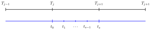
The source term is approximated using time samples per subinterval, as illustrated in Fig. 1.
The shifted IVP (8) can be decoupled into independent subproblems by the principle of superposition. To each subinterval we associate a part of the source term , defined for as
| (10) |
The expected parallel speedup is based on the observation that the solution to (8) is given by a variation-of-constant formula (see, e.g., [26]),
| (11) |
where the integrals can be evaluated independently and in parallel. More precisely, by exploiting the linearity of the problem we decompose the IVP (20) into independent subproblems,
| (12) | ||||
where is referred to as a subsolution of the total problem. The subproblems are independent and can be solved in parallel. We integrate the subproblem individually with the EBK method. Observe that the source is only nonzero on the subinterval . We follow the ideas of the Paraexp method [21] and note that the nonhomogeneous part of the ODE requires most of the computational work in the EBK method. An accurate SVD approximation of the source term (4) generally requires more singular values to be retained, increasing the dimensions of the block Krylov subspace (7). According to the principle of superposition, the solution of the original problem is then given as
| (13) |
The summation of the subsolutions, is the only communication required between the parallel processes. The parallel algorithm is summarized in Fig. 2. In principle, this algorithm is identical to the Paraexp method [21]. The only practical difference is that in our implementation both the nonhomogeneous and the homogeneous part of the subproblems are solved by the EBK method. The original version of the Paraexp method assumes a convential time integration method to solve the “difficult” nonhomogeneous part, and a Krylov subspace method for exponential integration of the homogeneous part. Our implementation of the Paraexp method is compared numerically with the original one in Section 3.2.
Finally, additional parallelism could be exploited within the block Krylov subspace method itself. If the block size is , then the matrix-vector products can be executed entirely in parallel, see [34, 46]. This approach could be applied in combination with the parallelization described in this section.
Given: , , , …
Solve:
for (in parallel)
Solve nonhomogeneous part of the ODE (12), for .
Solve homogeneous part of the ODE (12), for
end for
Construct solution , see (13).
2.3 Treatment of nonlinearities
The EBK method, designed to solve a linear system of nonhomogeneous ODEs (1), can be extended to handle nonlinear systems of ODEs by including the nonlinearities in the source term. The system is then solved iteratively, in such a way that the iterand is updated on the entire interval :
| (14) |
where denotes the iteration index. We proceed in a few steps. First, the problem is reduced to the form of Eq. (1). The nonlinear IVP is therefore approximated by evaluating the source term with the current iterand, . Because the current iterand is a known function, we can write the source term as an explicit function of time,
| (15) |
The resulting initial value problem is,
| (16) | ||||
This system is solved by the EBK method to achieve one iteration. This process is continued until the solution is sufficiently converged. This approach is similar to applying Picard or fixed-point iterations [42] on the nonlinear term. The source term can be further improved for nonlinear behaviour by using the Jacobian matrix, similar to a Newton–Rhapson method. In this case, we introduce the average Jacobian matrix,
| (17) |
which is averaged over the interval of integration . Generally, the solution varies in time and so does the Jacobian matrix. The nonlinear remainder, with respect to the time-averaged state, is contained in the source term. Using this correction, we then find the recursive relation,
| (18) | ||||
When converged, , the terms containing eventually disappear.
Remark 2.
The iteration (18) is well known in the literature on waveform relaxation methods [37, 38]. Its convergence is given, e.g., in [5, 42] and, in case of an inexact iteration, in [6]. These results, in particular, show that the iteration (18) converges superlinearly on finite time intervals if the norm of the matrix exponential of decays exponentially with , i.e., the eigenvalues of lie in the left half-plane.
2.4 Parallelization of nonlinear problems
Nonlinear IVPs are solved in an iterative way with the PEBK method. We follow the waveform relaxation approach [6, 33, 42], that is, the problem is solved iteratively on the entire time interval of interest, . The original problem is decomposed into a number of independent, “easier” subproblems on that can be solved iteratively, and in parallel.
At each iteration the nonlinear term is treated as source term, which gives us a linear system of ODEs that can be integrated in parallel, see Section 2.2. In the case of nonlinear problems, we take the average of the Jacobian matrix on each subinterval, which gives us the piecewise constant function for :
| (19) |
The IVP is then shifted with respect to the initial condition,
| (20) | ||||
where,
| (21) |
The shifted IVP (20) can be then solved in parallel. We follow an approach similar to the Paraexp method, as explained in Section 2.2. Here, we define
| (22) |
Now, the problem is decomposed into independent subproblems. The subsolutions result from convergence of obeying:
| (23) | ||||
| (24) |
which can be integrated with the EBK method. Here, we have introduced a second subindex to indicate the th subsolution at the th iteration. The total solution can then be updated according to the principle of superposition,
| (25) |
After each iteration, the solution is assembled, and the time-averaged Jacobian matrix is updated at each subinterval, according to Eq. (19). Note that for linear systems of ODEs, no iterations are required at all. The parallel algorithm is summarized in Fig. 5.
The parallel effiency of the EBK method is achieved by incorporating the parallelization within the iterations that are required to solve nonlinear IVPs. The differences between the serial and the parallel algorithm are illustrated as flow diagrams in Figures 3 and 4.
We consider the parallel efficiency in an idealized setting, and estimate a theoretical upper bound here, assuming that communication among the processors can be carried out very efficiently. The computational cost can then be simply estimated by the number of iterations required for the numerical solution to converge. Suppose the computation time of a single EBK iteration is . The maximum parallel speedup is then,
where is number of iterations for serial time integration, and for parallel time integration. The theoretical upper bound of the parallel efficiency is then,
| (26) |
High parallel efficiency can be achieved if the parallelization does not slow down the convergence of the numerical solution. As will be demonstrated in Section 4, we typically observe that is not significantly larger than , and a near-optimal efficiency is achieved in various relevant cases. For comparison, the parallel efficiency of the Parareal algorithm is formally bounded by [39]. In our case, this upper bound is improved by a factor . Parareal is an iterative method for the parallelization of sequential time integration methods, whereas the EBK method, for nonlinear problems, is an iterative method to start with, and its parallelization does not necessarily increase the total number of iterations. Note the PFASST method [17] has a similar estimate of parallel efficiency as the PEBK method.
Given: , , , …
Solve:
for
for (in parallel)
Calculate time-averaged Jacobian matrix , see (19).
Solve nonhomogeneous part linearized ODE (24), for .
Solve homogeneous part linearized ODE (24), for .
end for
Update solution following (25).
end for
3 Advection-diffusion equation
In this section, we present results of numerical tests where the space-discretized advection-diffusion equation is solved with the EBK method. We demonstrate the consistency and stability of the EBK method for the linear advection-diffusion equation, which is a PDE describing a large variety of transport phenomena [32]. The spatial discretization, using central finite differencing for sake of illustration, of the PDE yields a linear system of ODEs. The time integration can be parallelized as described in Section 2.2. We illustrate the principle of parallelization for different physical parameters of the advection-diffusion equation, before we move on to nonlinear PDEs in Section 4. Convergence of the numerical solution is observed for different values of the physical parameters.
In our implementation of the EBK method, the IVP projected onto the block Krylov subspace is solved with the function ode15s in MATLAB (2013b). The relative tolerance of the PEBK solver is denoted by tol. In our tests, the block Krylov subspace is restarted every 20 iterations. For the truncated SVD approximation (4), are chosen to be piecewise cubic polynomials, although other types of approximations are possible as well, and are not crucial for the performance of the PEBK method. The sample points per subinterval are Chebyshev nodes. This is not crucial but gives a slightly better approximation than with uniform sample points.
3.1 Homogeneous PDE
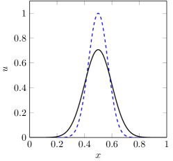
We consider the advection-diffusion equation with a short pulse initial condition, to clearly distinguish the seperate effects of advection and diffusion. The PDE and the periodic boundary conditions are as follows
| (27) | ||||
where is the advection velocity, and the diffusivity coefficient. Both parameters are constant in space and time. The PDE is first discretized in space with a second-order central finite difference scheme [41]. The corresponding semi-discrete system of ODEs is then
| (28) | ||||
where the matrix results from the discretization of the spatial derivatives, and represents both the diffusive and the advective term. In (28), the substitution has been applied, with being the vector function containing the values of the numerical solution on the mesh at time , with . The substitution leads to homogeneous initial conditions. In this case, the source term is constant in time, and its SVD polynomial approximation (4) is exact with . This allows us to focus on the two remaining parameters: the grid resolution and the tolerance of the EBK solver.
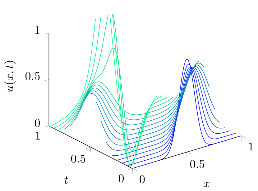
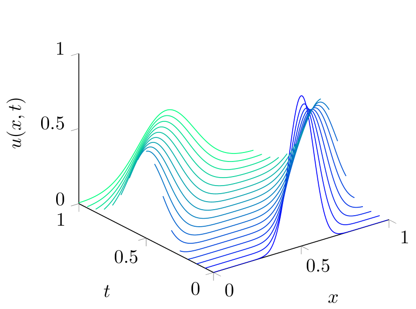
The linear IVP (28) is decoupled into independent subproblems by partitioning of the source term () on the time interval. The superposition of the subsolutions is illustrated in Fig. 6, in which the time interval of interest, , has been partitioned into four equal subintervals, to be integrated on four processors. The sum of the initial condition and the subsolutions gives the final solution on the entire time interval, see Section 2.2.
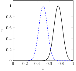
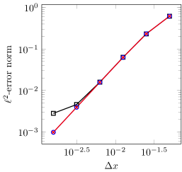
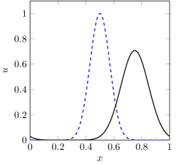
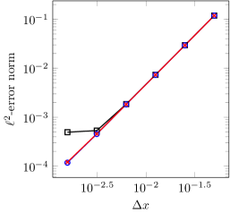
In the following numerical experiments, subintervals are used. The advection-diffusion equation is solved for three different combinations of and , see Fig. 7. The solutions are computed for different and . The discretization error is controlled by the time integration with , and by the spatial discretization with . The error of the numerical solution is measured in the relative -norm,
| (29) |
where the exact solution is on the mesh, i.e., it has the entries . The exact solution of Eq. (27) is
| (30) |
with coefficients
| (31) | ||||
| (32) |
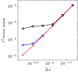
The coefficients are calculated using numerical quadrature with high precision. The error in (29) shows second-order convergence with , as expected from the truncation error of the finite difference scheme. The convergence plots show that we are able to control the error of the parallel time integration method. In this case, the final error can be made to depend only on the spatial resolution and the tolerance of the EBK method. Also, the EBK method has no principal restrictions on the timestep size, as it directly approximates the exact solution of Eq. (28) by Krylov subspace projections.
3.2 Parallel efficiency
In the previous examples, we solved homogeneous IVPs. Nonhomogeneous problems are generally more expensive to solve, because an accurate SVD approximation of the source term (4) requires more singular values, which increases the block width of the block Krylov subspace (7). Parallel speedup can then be expected by splitting the nonhomogeneous problem into subproblems (12), which require less individual effort to solve by the PEBK method. To measure the parallel efficiency of our algorithm for nonhomogeneous IVPs, we introduce a source term in the advection-diffusion equation
| (33) |
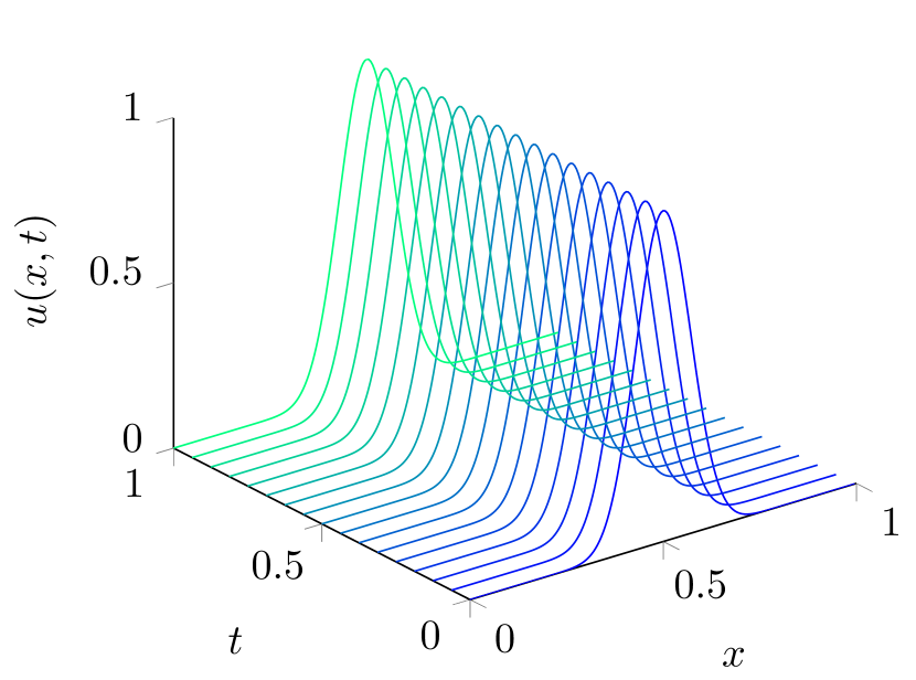
with , and . The source term is chosen such that the solution is a series of five travelling pulses
| (34) |
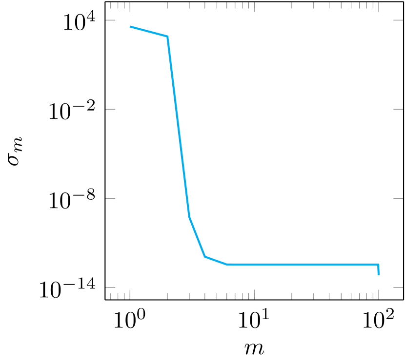
The mesh width of the spatial discretization is , such that the error due to the spatial discretization is small compared to the time integration error. The mesh width gives a semi-discrete system with a matrix, which is a suitable problem size for testing the EBK method. The tolerance of the EBK method is set to . The SVD polynomial approximation is constructed from 100 time samples per subinterval. The singular values are plotted in Fig. 9, which reveals that the first two singular values are several orders larger than the rest. Therefore, we retain only the first two singular values in the truncated SVD. The decay of singular values is guaranteed by the upper bound from Theorem 1. We have verified that the SVD approximation is sufficiently accurate, i.e., the approximation error, measured in the -norm, is less than the tolerance of the EBK method.
We compare the parallel efficiency of the Paraexp-EBK implementation with a convential implementation of the Paraexp algorithm [21], where the nonhomogeneous problem is integrated with the Crank–Nicolson (CN) scheme. The linear system is solved directly using MATLAB. The matrix exponential propagator, for the homogeneous problem in the Paraexp method, is realized with an Arnoldi method using the shift-and-invert technique [51].
In order to have a Courant number of one, we take (for and ). According to the Paraexp method, the time step size needs to be decreased in parallel computation by a factor [21], where is the order of the time integration method, in order to control the error. In case of the Crank–Nicolson scheme, we have .
As discussed in Section 2.2, there is no communication required between processors, except for the superposition of the solutions to the subproblems at the end. Therefore, we are able to test the parallel algorithm on a serial computer by measuring the computation time of each independent subproblem. The computation time of the serial time integration is denoted . For the parallel time integration, we measure the computation times of the nonhomogeneous and the homogeneous part of the subproblems separately, denoted by and respectively. The parallel speedup can then be estimated as
| (35) |
where we take the maximum value of and over all parallel processes. The timings of the EBK method and Paraexp are listed in Table 1.
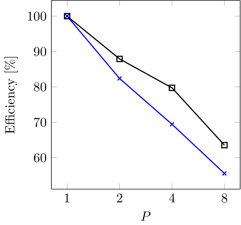
The parallel efficiency of both methods is illustrated in Figure 9. Note that the parallel efficiency of the standard Paraexp method steadily decreases, whereas the PEBK method maintains a constant efficiency level around . The decrease in efficiency of the standard Paraexp method is due to the reduced time step size in the Crank–Nicolson scheme, with respect to its serial implementation. The nonhomogeneous part of the subproblems requires more computation time as the number of processors increases.
The numerical test confirms the initial assumption that parallel speedup with the EBK method can be achieved by decomposing the originial problem into simpler independent subproblems (12). Furthermore, the Paraexp implementation using the EBK method, appears to be more efficient than one using a traditional time-stepping method.

| Serial | Parallel | ||||||
|---|---|---|---|---|---|---|---|
| Error | Error | Efficiency | |||||
| PEBK | 2 | 1.43e+00 | 3.05e-04 | 7.22e-01 | 6.44e-02 | 2.70e-04 | 91 |
| 4 | 2.81e+00 | 3.05e-04 | 7.23e-01 | 7.06e-02 | 2.68e-04 | 89 | |
| 8 | 5.59e+00 | 3.05e-04 | 7.40e-01 | 6.21e-02 | 2.88e-04 | 87 | |
| 16 | 1.14e+01 | 3.05e-04 | 7.30e-01 | 6.28e-02 | 3.22e-04 | 90 | |
| 32 | 2.27e+01 | 3.05e-04 | 7.33e-01 | 6.63e-02 | 3.65e-04 | 89 | |
| Paraexp | 2 | 2.15e+00 | 4.56e-04 | 1.29e+00 | 1.66e-02 | 4.10e-04 | 82 |
| 4 | 4.37e+00 | 4.56e-04 | 1.52e+00 | 1.28e-02 | 3.80e-04 | 71 | |
| 8 | 8.56e+00 | 4.56e-04 | 1.85e+00 | 1.24e-02 | 3.59e-04 | 58 | |
| 16 | 1.70e+01 | 4.56e-04 | 2.18e+00 | 1.31e-02 | 3.43e-04 | 49 | |
| 32 | 3.43e+01 | 4.56e-04 | 2.62e+00 | 1.16e-02 | 3.32e-04 | 41 | |
4 Burgers equation
In the previous section, the PEBK method was applied to a linear PDE. In this section, the performance of the PEBK method is tested on a nonlinear PDE, the viscous Burgers equation.
4.1 Travelling wave
Consider the viscous Burgers equation,
| (36) |
where denotes the diffusivity (or viscosity) coefficient. In the following experiments, we take , such that the problem is dominated by the nonlinear convective term. As in the previous example, the boundary conditions are periodic. Exact solutions to the Burgers equation can be found by the Cole–Hopf transformation [27]. In this test case, we construct a desired solution by introducing an appropriate source term, as shown for the advection-diffusion equation in Section 3.2. The the source term balances the dissipation of energy due to diffusion, and prevents the solution of vanishing in the limit .
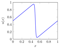
The Burgers equation is an important equation in fluid dynamics. It can be seen as a simplification of the Navier–Stokes equation, which retains the nonlinear convective term, . In the limit , the nonlinearity may produce discontinuous solutions, or shocks, so that a typical solution may resemble a sawtooth wave. A sawtooth wave can be represented by an infinite Fourier series. A smooth version of the sawtooth wave can be obtained by the modified Fourier series,
| (37) |
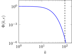
where is the wavenumber, a cutoff wavenumber, and is a smoothing function, which supresses the amplitudes associated to high wavenumbers:
| (38) |
Here, is the smoothing parameter. The smoothing function is motivated by the viscosity-dependent inertial spectrum of the Burgers equation found by Chorin & Hald [11]. The smoothing function for is shown in Figure 10(a). As the smoothing function rapidly decreases with wavenumber, we choose a cutoff wavenumber of . The value is found to produce a smooth version of a sawtooth wave, as shown in Figure 10(b).
We consider a wave travelling in the positive -direction by introducing the parametrization in (36). The source term is then readily found by substituting the chosen solution (37) into the Burgers equation (36),
| (39) |
The space derivatives in the Burgers equation are discretized with a second-order central finite difference schemes, using a uniform mesh width . The error of the numerical solution is again measured in the relative -norm, cf. (29).
The tolerance of the PEBK method is set to . The SVD approximation of the source term, which includes the nonlinear term, is constructed from samples per subinterval, and reveals that singular values are sufficient in the truncated SVD, so that the error of the SVD approximation is less than the tolerance of the PEBK method.
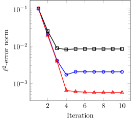
The nonlinear system of ODEs is solved iteratively, as outlined in Section 2.3. Figure 11 shows the error history at different grid resolutions. Here, the error converges to a value that depends on the mesh width. In other words, the final error of the time integration method is much smaller than the error due to the spatial discretization.
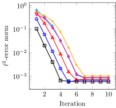
The PEBK method is parallelized as discussed in Section 2.4. The time interval can be partitioned into subintervals with a uniform subinterval size . In the following experiment, the complete time interval is extended with each subinterval added, . The mesh width is . Figure 12(a) shows that increasing the number of processors and hence the simulated time, generally increases the number of iterations required to achieve the same level of accuracy. The increased number of required iterations implies a decrease in theoretical parallel efficiency, which can be estimated by the ratio , see (26).
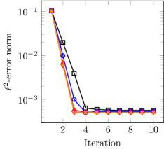
Next, the final time is kept constant, and the subinterval size reduces with an increase in the number of processors, . Figure 12(b) shows that the number of iterations is roughly independent of the number of processors, i.e., in this case, the parallel efficiency, , does not decrease with . Parallel speedup might also be improved by the fact that the SVD approximation converges faster on smaller subintervals, see Theorem 1. That is, fewer singular values have to be retained in the truncated SVD in order to achieve a certain accuracy. Also, the number of samples of the source term could be decreased on smaller subintervals.
4.2 Parallel efficiency
In this section, we test the parallel efficiency of the PEBK method for the viscous Burgers equation. In the following experiments, the source term is chosen such that the solution of the spatially discretized system is equal to the exact solution described in Section 4.1. In other words, the source term accounts for the error by the spatial discretization, and we measure only the error due to the time integration. The spatial discretization is here performed with a mesh width of .
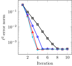
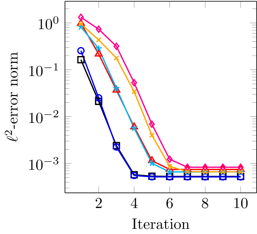
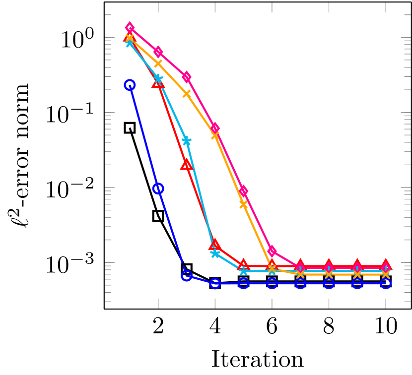
If the subinterval size, , is fixed, the number of iterations generally increases in case the number of processors increases, see Fig. 12. Increasing the number of iterations would reduce the parallel efficiency, according to (26). We therefore fix the final time , such that the subinterval size decreases with increasing . Also, the total number of samples over is fixed, such that the local number of samples decreases with increasing . To keep the global distribution of samples constant in the parallel computations, the local sample points are uniformly distributed instead of Chebyshev points as used in previous experiments. In our experiments, we use and . Furthermore, the number of (retained) singular values is , and the tolerance of the EBK method is set to . The error history for different is shown in Fig. 13. The results show that the convergence rate of the PEBK method can improve by increasing . The nonlinear corrections, see (18), appear to be more effective on smaller subintervals.
As opposed to the linear problem in Section 3.2, communication between the parallel processes is here required because of the waveform relaxation method. The parallel communication overhead is assumed to be very small, such that the parallel computations can be emulated on a serial computer. Per iteration of the PEBK method, the computation time of each individual process is measured, after which the maximum is stored, i.e., the computation time of the slowest process. The total computation time of the PEBK method is then taken as the sum, over the total number of iterations performed, of the maxima. In this experiment, we have measured a total of ten PEBK iterations.
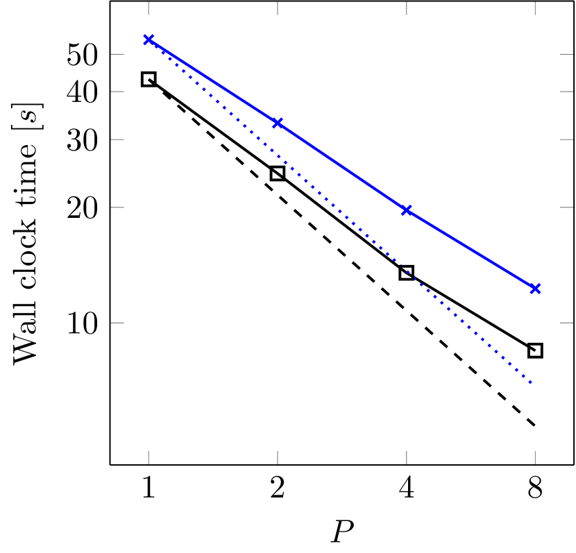
The computation times for and are shown in Fig. 14(a), which clearly illustrate a parallel speedup. The slightly higher timings of could be attributed to the increased stiffness of the problem. Figure 14(b) shows that the parallel efficiency of the PEBK method steadily decreases with the number of (virtual) processors, . There is no significant difference between the performance of the method at these two values of the viscosity coefficient. The parallel efficiency might even be further tuned in practice, based on the previous observation that the required number of iterations could decrease with higher . Also, the number of singular values, , could possibly be reduced on smaller subintervals, based on (1), which would further enhance the potential parallel speedup.
The PFASST algorithm [17] shows a good parallel efficiency for the viscous Burgers equation as well. It is unknown whether changing the viscosity coefficient has an impact on the performance of PFASST. Our observations point in the direction of a good parallel efficiency of the PEBK method for simulations of the Navier–Stokes equation at high Reynolds numbers. For these problems there is a high demand for highly efficient parallel solvers [53]. The Parareal algorithm was for example reported to perform poorly in advection-dominated problems [18, 49].
4.3 Multiscale example
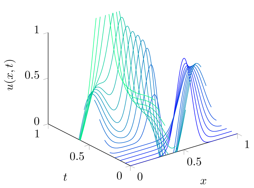
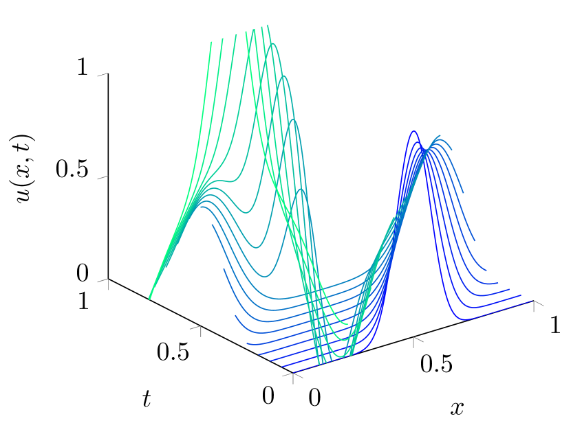
Turbulent flow is a multiscale phenomenon that is characterized by a wide range of length and time scales. In case of the Burgers equation, we can emulate such a solution by combining two functions that are periodic in both space and time, e.g.,
| (40) |
The solution features a large scale mode with wavenumber one, and a smaller scale mode with wavenumber . This combination allows the construction of an arbitrarily wide dynamic range. The factor is included in compliance with an assumed energy distribution of [11], where is the Fourier transform,
| (41) |
where we have used the fact that the solution is periodic in space and time. The previous experiment, see Fig. 12(a), is repeated for the manufactured solution (40) with different values of . Figure 15 illustrates that widening the spectrum does not significantly affect the convergence of the PEBK iterations. Remarkably, the curves appear to form pairs based on .
5 Conclusions
We propose an implementation of the Paraexp method with enhanced parallelism based on the exponential block Krylov (EBK) method. Furthermore, the method, Paraexp-EBK (PEBK), is extended to solve nonlinear PDEs iteratively by a waveform relaxation method. The nonlinear terms are represented by a source term in a nonhomogeneous linear system of ODEs. Each iteration the source term is updated with the latest solution. The convergence of the iterative process can be accelerated by adding a correction term based on the Jacobian matrix of the nonlinear term. Each iteration the initial value problem can then be decoupled into independent subproblems, which can be solved parallel in time. Essentially, we implement the Paraexp method within a waveform relaxation approach in order to integrate nonlinear PDEs. Also, the Paraxp-EBK (PEBK) method is used to integrate both the homogeneous and the nonhomogeneous parts of the subproblems. This is in contrast to the original Paraexp method, which assumes a convential time integration method for the nonhomogeneous parts.
The PEBK method is tested on the advection-diffusion equation for which we demonstrate the parallelization concept for linear PDEs. The parallelization also works in cases without diffusion present, in which the PDE is purely hyperbolic. The parallel efficiency is compared with a Crank–Nicolson (CN) scheme parallelized with the Paraexp algorithm. The parallel efficiency of the PEBK method remains roughly constant around . On the other hand, the parallel efficiency of the CN/Paraexp combination steadily decreases with the number of processors.
As a model nonlinear PDE, the viscous Burgers equation is solved. The number of waveform relaxation iterations required for a certain error tolerance increases, when the relative importance of nonlinearity grows by decreasing the viscosity coefficient. Good parallel efficiency of the EBK method was observed for different values of the viscosity coefficient. Since the nonlinear convective term in the Burgers equation is shared by the Navier–Stokes equation, the presented results give a hint of the potential of the PEBK method as an efficient parallel solver in turbulent fluid dynamics, where nonlinearity plays a key role. The question remains how to treat the pressure in the incompressible Navier–Stokes equation, which enforces the incompressibility constraint on the velocity field (see for possible approaches in [15, 43]). This will be explored in future work.
References
- [1] M. Afanasjew, M. Eiermann, O. G. Ernst, and S. Güttel. Implementation of a restarted Krylov subspace method for the evaluation of matrix functions. Linear Algebra Appl., 429:2293–2314, 2008.
- [2] M. Botchev. A block Krylov subspace time-exact solution method for linear ordinary differential equation systems. Numerical linear algebra with applications, 20(4):557–574, 2013.
- [3] M. Botchev, G. Sleijpen, and A. Sopaheluwakan. An SVD-approach to Jacobi–Davidson solution of nonlinear Helmholtz eigenvalue problems. Linear Algebra and its Applications, 431(3):427–440, 2009.
- [4] M. A. Botchev, I. Faragó, and A. Havasi. Testing weighted splitting schemes on a one-column transport-chemistry model. Int. J. Environment and Pollution, 22(1/2):3–16, 2004.
- [5] M. A. Botchev, V. Grimm, and M. Hochbruck. Residual, restarting, and Richardson iteration for the matrix exponential. SIAM Journal on Scientific Computing, 35(3):A1376–A1397, 2013.
- [6] M. A. Botchev, I. V. Oseledets, and E. E. Tyrtyshnikov. Iterative across-time solution of linear differential equations: Krylov subspace versus waveform relaxation. Computers & Mathematics with Applications, 67(12):2088–2098, 2014. \urlhttp://dx.doi.org/10.1016/j.camwa.2014.03.002.
- [7] M. A. Botchev and H. A. van der Vorst. A parallel nearly implicit scheme. Journal of Computational and Applied Mathematics, 137:229–243, 2001.
- [8] K. Burrage. Parallel and sequential methods for ordinary differential equations. The Clarendon Press Oxford University Press, New York, 1995. Oxford Science Publications.
- [9] A. Cella and M. Lucchesi. Space-time finite elements for the wave propagation problem. Meccanica, 10(3):168–170, 1975. \urlhttp://dx.doi.org/10.1007/BF02149028.
- [10] E. Celledoni and I. Moret. A Krylov projection method for systems of ODEs. Applied numerical mathematics, 24(2):365–378, 1997.
- [11] A. J. Chorin and O. H. Hald. Viscosity-dependent inertial spectra of the Burgers and Korteweg–deVries–Burgers equations. Proceedings of the National Academy of Sciences of the United States of America, 102(11):3921–3923, 2005.
- [12] J. J. B. de Swart. Parallel Software for Implicit Differential Equations. PhD thesis, University of Amsterdam, Nov. 1997. ISBN 90-74795-77-3.
- [13] S. V. Dolgov, B. N. Khoromskij, and I. V. Oseledets. Fast solution of parabolic problems in the tensor train/quantized tensor train format with initial application to the fokker–planck equation. SIAM Journal on Scientific Computing, 34(6):A3016–A3038, 2012. \urlhttp://dx.doi.org/10.1137/120864210.
- [14] J. Dongarra et al. The international exascale software project roadmap. International Journal of High Performance Computing Applications, page 1094342010391989, 2011.
- [15] W. Edwards, L. Tuckerman, R. Friesner, and D. Sorensen. Krylov methods for the incompressible Navier–Stokes equations. Journal of Computational Physics, 110(1):82 – 102, 1994.
- [16] M. Eiermann, O. G. Ernst, and S. Güttel. Deflated restarting for matrix functions. SIAM J. Matrix Anal. Appl., 32(2):621–641, 2011.
- [17] M. Emmett and M. Minion. Toward an efficient parallel in time method for partial differential equations. Communications in Applied Mathematics and Computational Science, 7(1):105–132, 2012.
- [18] P. F. Fischer, F. Hecht, and Y. Maday. A Parareal in time semi-implicit approximation of the Navier–Stokes equations. In Domain decomposition methods in science and engineering, pages 433–440. Springer, 2005.
- [19] M. Gander and S. Vandewalle. Analysis of the Parareal Time‐-Parallel Time‐-Integration Method. SIAM Journal on Scientific Computing, 29(2):556–578, 2007.
- [20] M. J. Gander. Analysis of the parareal algorithm applied to hyperbolic problems using characteristics. Boletin de la Sociedad Espanola de Matemática Aplicada, 42:21–35, 2008.
- [21] M. J. Gander and S. Güttel. Paraexp: A parallel integrator for linear initial-value problems. SIAM Journal on Scientific Computing, 35(2):C123–C142, 2013.
- [22] T. Göckler and V. Grimm. Uniform approximation of -functions in exponential integrators by a rational Krylov subspace method with simple poles. SIAM Journal on Matrix Analysis and Applications, 35(4):1467–1489, 2014. \urlhttp://dx.doi.org/10.1137/140964655.
- [23] G. H. Golub and C. F. Van Loan. Matrix computations. Johns Hopkins University, Press, Baltimore, MD, USA, pages 374–426, 1996.
- [24] W. Hackbusch. Parabolic multigrid methods. In Computing methods in applied sciences and engineering, VI (Versailles, 1983), pages 189–197. North-Holland, Amsterdam, 1984.
- [25] M. Hochbruck and J. Niehoff. Approximation of matrix operators applied to multiple vectors. Mathematics and Computers in Simulation, 79(4):1270–1283, 2008.
- [26] M. Hochbruck and A. Ostermann. Exponential integrators. Acta Numerica, 19:209–286, 2010.
- [27] E. Hopf. The partial differential equation . Communications on Pure and Applied mathematics, 3(3):201–230, 1950.
- [28] R. A. Horn and C. R. Johnson. Matrix Analysis. Cambridge University Press, 1986.
- [29] R. A. Horn and C. R. Johnson. Topics in Matrix Analysis. Cambridge University Press, 1991.
- [30] G. Horton and S. Vandewalle. A space-time multigrid method for parabolic partial differential equations. SIAM J. Sci. Comput., 16(4):848–864, 1995. \urlhttp://dx.doi.org/10.1137/0916050.
- [31] T. J. R. Hughes and G. M. Hulbert. Space-time finite element methods for elastodynamics: formulations and error estimates. Comput. Methods Appl. Mech. Engrg., 66(3):339–363, 1988. \urlhttp://dx.doi.org/10.1016/0045-7825(88)90006-0.
- [32] W. Hundsdorfer and J. G. Verwer. Numerical solution of time-dependent advection-diffusion-reaction equations, volume 33. Springer Science & Business Media, 2013.
- [33] E. Lelarasmee, A. E. Ruehli, and A. Sangiovanni-Vincentelli. The waveform relaxation method for time-domain analysis of large scale integrated circuits. Computer-Aided Design of Integrated Circuits and Systems, IEEE Transactions on, 1(3):131–145, July 1982.
- [34] G. Li. A block variant of the GMRES method on massively parallel processors. Parallel Computing, 23(8):1005–1019, 1997.
- [35] J.-L. Lions. Équations différentielles opérationnelles et problèmes aux limites. Die Grundlehren der mathematischen Wissenschaften, Bd. 111. Springer-Verlag, Berlin-Göttingen-Heidelberg, 1961.
- [36] J.-L. Lions, Y. Maday, and G. Turinici. Résolution d’edp par un schéma en temps «pararéel ». Comptes Rendus de l’Académie des Sciences - Series I - Mathematics, 332(7):661 – 668, 2001.
- [37] C. Lubich and A. Ostermann. Multi-grid dynamic iteration for parabolic equations. BIT Numerical Mathematics, 27:216–234, 1987. 10.1007/BF01934186.
- [38] U. Miekkala and O. Nevanlinna. Convergence of dynamic iteration methods for initial value problems. SIAM Journal on Scientific and Statistical Computing, 8(4):459–482, 1987.
- [39] M. Minion. A hybrid parareal spectral deferred corrections method. Communications in Applied Mathematics and Computational Science, 5(2):265–301, 2011.
- [40] I. Moret and P. Novati. RD rational approximations of the matrix exponential. BIT, 44:595–615, 2004.
- [41] K. W. Morton and D. F. Mayers. Numerical solution of partial differential equations: an introduction. Cambridge university press, 2005.
- [42] O. Nevanlinna. Remarks on Picard-Lindelöf iteration. BIT Numerical Mathematics, 29(2):328–346, 1989.
- [43] C. K. Newman. Exponential Integrators for the Incompressible Navier–Stokes Equations. PhD thesis, Virginia Polytechnic Institute and State University, 2004.
- [44] A. R. Newton and A. L. Sangiovanni-Vincentelli. Relaxation-based electrical simulation. IEEE Transactions on Electron Devices, 30(9):1184–1207, 1983.
- [45] J. Niehoff. Projektionsverfahren zur Approximation von Matrixfunktionen mit Anwendungen auf die Implementierung exponentieller Integratoren. PhD thesis, Mathematisch-Naturwissenschaftlichen Fakultät der Heinrich-Heine-Universität Düsseldorf, December 2006.
- [46] A. Nikishin and A. Y. Yeremin. Variable block CG algorithms for solving large sparse symmetric positive definite linear systems on parallel computers, I: General iterative scheme. SIAM Journal on Matrix Analysis and Applications, 16(4):1135–1153, 1995.
- [47] D. Ruprecht and R. Krause. Explicit parallel-in-time integration of a linear acoustic-advection system. Computers & Fluids, 59:72–83, 2012.
- [48] G. A. Staff and E. M. Rønquist. Stability of the parareal algorithm. In Domain decomposition methods in science and engineering, pages 449–456. Springer, 2005.
- [49] J. Steiner, D. Ruprecht, R. Speck, and R. Krause. Convergence of Parareal for the Navier–Stokes equations depending on the Reynolds number. In Numerical Mathematics and Advanced Applications-ENUMATH 2013, pages 195–202. Springer, 2015.
- [50] H. Tal-Ezer. On restart and error estimation for Krylov approximation of . SIAM J. Sci. Comput., 29(6):2426–2441, 2007.
- [51] J. van den Eshof and M. Hochbruck. Preconditioning Lanczos approximations to the matrix exponential. SIAM J. Sci. Comput., 27(4):1438–1457, 2006.
- [52] P. J. van der Houwen and B. P. Sommeijer. CWI contributions to the development of parallel Runge-Kutta methods. CWI Quarterly, 11(1):33–53, 1998. Solving differential equations on parallel computers.
- [53] E. P. van der Poel, R. Ostilla-Mónico, J. Donners, and R. Verzicco. A pencil distributed finite difference code for strongly turbulent wall-bounded flows. Computers & Fluids, 116(0):10–16, 2015.
- [54] J. J. W. van der Vegt and H. van der Ven. Space-time discontinuous Galerkin finite element method with dynamic grid motion for inviscid compressible flows. I. General formulation. J. Comput. Phys., 182(2):546–585, 2002.
- [55] J. G. Verwer and J. M. Sanz-Serna. Convergence of method of lines approximations to partial differential equations. Computing, 33(3-4):297–313, 1984.
- [56] J. White, F. Odeh, A. L. Sangiovanni-Vincentelli, and A. Ruehli. Waveform relaxation: Theory and practice. Technical Report UCB/ERL M85/65, EECS Department, University of California, Berkeley, 1985.
- [57] J. Zhu. A new parallel algorithm for the numerical solutions of time dependent partial differential equations (unpublished note). Engineering Research Center, Mississippi State University, 2000.