Can recurrence networks show small-world property?

Abstract

Recurrence networks are complex networks, constructed from time series data, having several practical applications. Though their properties when constructed with the threshold value $\epsilon$ chosen at or just above the percolation threshold of the network are quite well understood, what happens as the threshold increases beyond the usual operational window is still not clear from a complex network perspective. The present Letter is focused mainly on the network properties at intermediate-to-large values of the recurrence threshold, for which no systematic study has been performed so far. We argue, with numerical support, that recurrence networks constructed from chaotic attractors with $\epsilon$ equal to the usual recurrence threshold or slightly above cannot, in general, show small-world property. However, if the threshold is further increased, the recurrence network topology initially changes to a small-world structure and finally to that of a classical random graph as the threshold approaches the size of the strange attractor.

1 Introduction

In the last two decades, complex network theory has emerged as a popular tool for analyzing complex and spatially extended systems [1, 2, 3]. It has found applications in a wide range of fields including sociology [4, 5], communication [6, 7] and biological sciences [8, 9]. The theory of complex networks initially started with random graphs (RG) studied in detail by Erdős and Rényi (E-R) [10]. For RGs, there is a fixed probability $p$ for two nodes being connected and one can show that for a sufficiently large number of nodes $N$, the degree distribution $P(k)$ tends to a Poissonian.

The E-R model guided our thinking about complex networks for many decades until the discovery by Barabasi and co-workers [11, 12] nearly two decades back that the topology and structure of most networks around us are radically different. For example, many networks in the real world such as, the World Wide Web (WWW) [13], networks of social interactions [14], protein and metabolic networks [15] and technological networks [16], tend to obey certain self-organizing principles in their evolution either due to some inherent property of the system or due to the nature of human interactions as in social networks. The topology of such networks shows a scale invariance with the degree distribution obeying a power law, $P(k)\propto k^{-\gamma}$, and the value of $\gamma$ is found to be typically between $2$ and $3$. The discovery of such scale-free (SF) networks triggered a lot of interest in the theory of complex networks.

Along with the discovery of SF networks, the concept of small-world (SW) networks was introduced by Watts and Strogatz [17]. Though the classical RGs are amenable to a great deal of mathematical analysis, they are poor models as far as real networks are concerned. Firstly, they show poor clustering and their clustering coefficient (CC) is directly proportional to $p$. Secondly, for a given $p$, as the number of nodes $N$ increases, the average degree $<k>$ also increases correspondingly. Consequently, for $p$ above a threshold value, the characteristic path length (CPL) of RGs remains very small and independent of $N$.

Watts and Strogatz (W-S) showed that, starting from a ring lattice of $N$ nodes with nearest neighbour coupling and randomly re-wiring a small fraction $\beta$ of edges, results in a complex network with high CC compared to the RG and small CPL comparable to that of a RG for a range of values of $\beta$. Moreover, for such networks, as $N$ increases, the CPL increases only as $log$ $N$. Thus the W-S model displays many characteristic properties of real world networks and provides one possibility of obtaining the SW property, often found in real world networks, with different levels of complexity by tuning $\beta$.

The above developments resulted in complex networks and the related measures being applied as tools in many areas of research. The most recent among them is the analysis of time series from dynamical systems using statistical measures of complex networks. To study many dynamical processes in the real world, one often resorts to the analysis of time series obtained from the system. An area of special interest is where the underlying system appears to show deterministic nonlinear behavior. The methods and measures of nonlinear time series analysis and chaos theory [18, 19] are commonly used in such cases. In the last few years, measures based on complex networks have gained a lot of importance in nonlinear time series analysis. All such measures propose a mapping from the time series domain to the network domain and then proceed to characterize the dynamical system in terms of the statistical measures of the resulting complex network. By doing this, one expects to resolve complimentary features that are not captured by conventional methods of time series analysis, especially the structural and topological properties of the underlying chaotic attractor.

Even though several methods have been proposed [20, 21, 22] to convert time series into networks, an approach incorporating the generic property of recurrence [23] of a dynamical system has been prominently applied for the conversion of time series into networks. In this method, the time series is first embedded in a suitable dimension $M$ using time delay co-ordinates [24] to reconstruct the attractor. Every point on the attractor is identified as a node and the network can be constructed in two ways, either by taking a fixed number of nearest neighbours [25] or by taking a fixed hyper-sphere of radius $\epsilon$ with the point as the centre. In this work, we consider the second method for the construction of the network where a reference node $\imath$ is connected to another node $\jmath$ if the Euclidean distance $d_{ij}$ between the corresponding points on the attractor in the reconstructed space is less than or equal to the recurrence threshold $\epsilon$, that is, if $d_{ij}\leq\epsilon$. The resulting complex network, called the $\epsilon$ - recurrence network or simply recurrence network (RN) [26, 27], has been shown to have great potential for a wide range of practical applications, from identifying critical transitions in dynamical systems [28] to the classification of cardio-vascular time series [29]. Note that, by construction, the RN is an undirected and unweighted graph with a symmetric and binary adjacency matrix $\mathcal{A}$, with elements $A_{ij}=1$ or $0$, depending on whether the two nodes $\imath$ and $\jmath$ are connected or not.

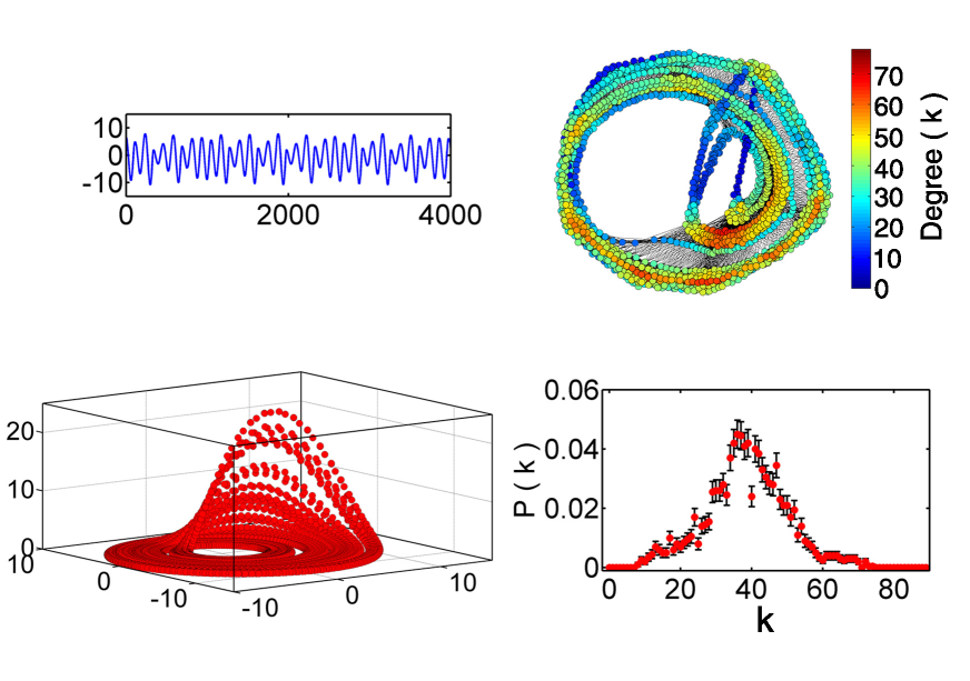
Figure 1: Construction of the RN from the time series of the standard Rössler attractor’s $y$ - component using time step $\Delta t=0.05$ with time delay $\tau=24$ and $M=3$. The time series and the embedded attractor are shown (top and bottom, respectively) in the left panel while the RN and its degree distribution are shown in the right panel. The RN is constructed taking every point on the attractor as a node and connecting every node to all other nodes within a recurrence threshold of $\epsilon=0.1$ (see text). Error bars of $P(k)$ originate from the fact that for a network with $N$ nodes, the number $n$ of nodes with a given degree $k$ has a standard error of $\sqrt{n}(k)$. For $n(k)\rightarrow 0$, its value is normalised to $1$, the minimum count.

Though RNs and related statistical measures are widely applied in nonlinear time series analysis, their properties, as the threshold is increased, are not fully understood from a complex network perspective. It is well known that all RNs have two properties in common. Firstly, the degree distribution of every RN is unique and is closely related to the probability density variations over the embedded attractor from which it is mapped [30]. We will discuss this in detail below. Secondly, there is an absence of long range connections as the maximum edge length is limited by the recurrence threshold $\epsilon$. By definition, RNs are random geometric graphs (RGG) in the considered system’s phase space [30, 31, 32]. Here RGGs are RGs where each vertex is randomly assigned co-ordinates in some metric space according to some prescribed probability distribution function, and vertices are connected if and only if they are separated by less than a certain maximum distance [33].

In this Letter, we numerically investigate the specific properties of RNs using three primary measures of a complex network, the degree distribution, the CC and the CPL. In particular, we consider the range of threshold values beyond the small operational window usually used for the construction of the RN and check whether the resulting network can show the properties of either RGs or SF networks or behave as a small-world network.

2 Numerical Results

All numerical simulations are done using $N=2000$ nodes, unless otherwise mentioned. For the construction of SF networks, we use the specific scheme of preferential attachment discussed in detail in [34]. Here we start with a small number of nodes $m_{0}$. A new node is then added which gets connected to $m$ number of existing nodes. This process is repeated, increasing the number of edges by $m$ for each newly connected node. By changing either $m_{0}$ or $m$ we can construct SF networks with different $\gamma$. Here we do both and construct the SF networks using 3 values for $m_{0}$ (2, 4 and 10) and in each case, use 3 different values for $m$, namely, 1, 2 and 4. Moreover, the RGs are constructed for different values of $p$. Time series from several standard low-dimensional chaotic systems are used for the construction of RNs. For continuous systems (flows) in 3D, we use the embedding dimension $M=3$ and for discrete systems (maps) in 2D, we use $M=2$. For all systems, we use the time series from the $y$ - component and for all continuous systems, the time step $\Delta t$ used for numerical integration is $0.05$ with the time delay computed by the automated algorithmic scheme proposed by us [35]. The values of time delay used for the Rössler, Lorenz, Duffing and Ueda systems are $24$, $6$, $25$ and $13$ respectively.

To get a quantitatively comparable value for the percolation threshold $\epsilon$ and to make the comparison between systems possible, we first transform the time series to a uniform deviate so that the size of the reconstructed attractor is re-scaled into a unit cube in $M$ dimensions. This transformation is not a trivial rescaling as it stretches the embedded attractor uniformly in all directions. We have already shown [35, 36] how effective this transformation is in computing conventional measures such as, correlation dimension $D_{2}$ and entropy $K_{2}$, for low as well as high-dimensional systems from time series [37]. As a result of the uniform deviate transformation, we have found that it is possible to have a small identical range of recurrence threshold $\Delta\epsilon$, that can be taken as the operational window for constructing the RN from time series of different systems for a given embedding dimension $M$ [38]. Here we choose the value of $\epsilon$ as the minimum of this range where the giant component of the RN just appears, as suggested by Donges et al. [32]. The value of $\epsilon$ is found to be $0.06$ for $M=2$ and $0.1$ for $M=3$ for $N\leq 10000$ as discussed in detail in [38]. The RN from a random (white noise) time series is also constructed using $M=3$ (for comparison with the RNs from chaotic systems) whose degree distribution is Poissonian with $<k>\approx 7$ for the selected $\epsilon$. We find that this distribution coincides with the degree distributions of a RG for $2000$ nodes with $p=0.0035$ and a RGG in $3$ dimensions with the spatial range of connections limited to the same threshold $\epsilon=0.1$ as that of the RN. To draw the connection with the percolation threshold of the RN, one can refer to [32]. In Fig. 1, we show the construction of a typical RN from a standard Rössler attractor time series. The node degrees of the RN vary over a wide range determined by the local probability density variations over the attractor. Specifically, the topology of the RN closely resembles that of the embedded attractor, with nodes corresponding to regions of high probability density in the attractor having higher degree in the RN and vice versa. This is evident from Fig. 1.

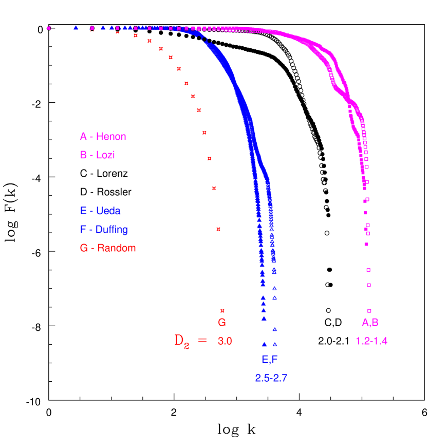
Figure 2: Cumulative degree distribution of RNs from several low-dimensional chaotic attractors and a random time series. The chaotic attractors are the Hénon (open square), Lozi (solid square), Lorenz (open circle), Rössler (solid circle), Duffing (open triangle) and Ueda (solid triangle) systems whose $D_{2}$ ranges are also indicated. The parameters used for all the systems are given in [39]. We observe that the position where $F(k)$ decreases sharply follows a pattern in accordance with the dimension of the attractor.

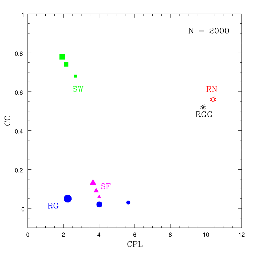
Figure 3: CPL-CC combined plot for different classes of networks with $2000$ nodes in all cases except the W-S network. We show the results for $3$ SF networks (solid triangles) with $\gamma=2.28,2.49,2.67$, $3$ RGs (solid circles) with link probability $p=0.002,0.0035,0.02$ and $3$ W-S small-world networks (solid squares) with $100$ nodes (to reduce computation time and memory) using $\beta=0.04,0.05,0.06$. In all cases, the size of the symbols increases with the values of $\gamma$, $p$ and $\beta$ respectively. The open star on the right side corresponds to the RN from a random time series and the asterisk corresponds to a RGG with the range of connection limited to that of the RNs in $3$ dimension, namely, $\epsilon=0.1$. These two networks are completely different from the other networks in terms of CPL-CC values.

As the dynamical system evolves, the probability density over the attractor is preserved. The degree $k_{i}$ of a reference node $\imath$ represents the local connectivity of the RN and corresponds to the local phase space density around the reference point in the attractor. It has already been shown [26, 38] that the local probability density variation is reflected in the degree distribution of the RN:

$${{k_{i}}\over{N}}\propto p(\vec{r}_{i})$$ (1)

for a given $M$, where $p(\vec{r}_{i})$ is the invariant density around the point $\vec{r}_{i}$. In the light of this equation, $k_{i}/N$ can be called the degree density [31]. The above equation tells us that the distribution in terms of the degree density remains invariant for a given attractor as has been explicitly shown by us earlier [38].

Due to this close connection with the invariant density, the degree distribution also carries important structural information on the corresponding chaotic attractor in a subtle manner. To show this explicitly, we consider the cumulative degree distribution of the RNs from several low-dimensional chaotic attractors. This representation is often used in the analysis of power-law degree distributions to retrieve the scaling that is not visible in the power-law tail. It has been extensively discussed in the literature [2] in connection with the analysis of SF networks and is defined as

$$F(k)=\sum_{k^{{}^{\prime}}=k}^{k_{max}}P(k^{{}^{\prime}})$$ (2)

It can be shown that if $P(k)$ is a power-law with exponent $\gamma$, then $F(k)$ will also follow a power-law with exponent $\gamma-1$. Here we make use of $F(k)$ only to get a better comparison between the degree distributions of various chaotic attractors.

In Fig. 2, we show the variation of $log$ $F(k)$ as a function of $log$ $k$ for RN from several low-dimensional chaotic attractors and random time series. The parameters used for the generation of all the chaotic attractors are given in the Appendix of [39]. In all cases, we use the $y$ - component of the system with time step $0.05$ for continuous systems. Note that the position of the tail of the distribution follows a pattern in accordance with the dimension $D_{2}$ of the attractor. To get a possible explanation for this observation, we have studied the actual distribution $P(k)$ of the RNs. In all cases, there is a range of $k$ values and a particular $k$ value, say $k^{\ast}$, at which $P(k)$ has a maximum value. The cumulative distribution starts decreasing sharply as $k$ exeeds $k^{\ast}$. Now, the value of $k^{\ast}$ increases with the range of $k$ values which, in turn, depends on the clustering of points on the attractor, as the attractor is converted into the network. For Hénon and Lozi attractors, the clustering is maximum as they are characterized by a lower $D_{2}$ value and consequently the range of $k$ values is maximum. This makes their profile getting shifted to extreme right. As $D_{2}$ increases, the range of $k$ values and hence $k^{\ast}$ decreases due to the rescaling of all systems to the unit cube, shifting the tail to lower $k$ values. For the random time series, when computed from a finite time series with embedding dimension $M$, we get $D_{2}=M$ and the range is minimum with $k^{\ast}=<k>$ and hence the tail of $F(k)$ is located at the extreme left. The above argument is supported by numerical results from earlier studies [26], if the local clustering coefficient can be understood analytically from the theory of random geometric graphs as being associated to a “mean local clustering dimension” defined in [31], which should behave similar to the classical correlation dimension $D_{2}$ considered here.

Next, we consider how the RNs are different with respect to the other two measures, CC and CPL. We generate an ensemble of SF networks with different $\gamma$ values using the specific scheme of preferential attachment as mentioned above and RGs with different link probability $p$. The CPL is defined by the equation

$$<l>={{1}\over{N(N-1)}}\sum_{i,j}^{N}l_{ij}$$ (3)

where $l_{ij}$ is the shortest path length for all pairs of nodes $(\imath,\jmath)$ in the network. The CC of the network is defined through a local clustering coefficient $c_{v}$ which measures the probability that two randomly chosen neighbours of a given vertex $v$ are mutually linked. For finite graphs, this is estimated [31] in terms of relative frequency of links between the neighbouring vertices for the node $v$.

$$c_{v}={{\sum_{i,j}A_{vi}A_{ij}A_{jv}}\over{k_{v}(k_{v}-1)}}$$ (4)

The average value of $c_{v}$ is taken as the CC of the whole network:

$$CC={{1}\over{N}}\sum_{v}c_{v}$$ (5)

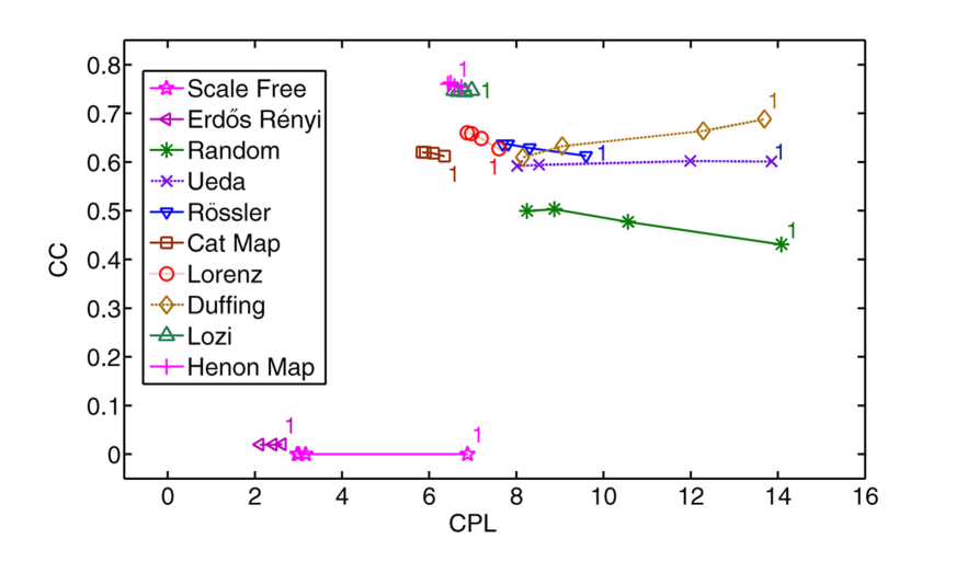
Figure 4: CPL-CC values for RNs generated from several low-dimensional chaotic attractors and random time series for $4$ different values of $N$, namely, $1000,2000,5000$ and $10000$ with the point denoted as $1$ representing $N=1000$. For comparison, values for a RG (with $p=0.004$) and a SF network (with $\gamma=2.162$) with the same $N$ values are also shown.

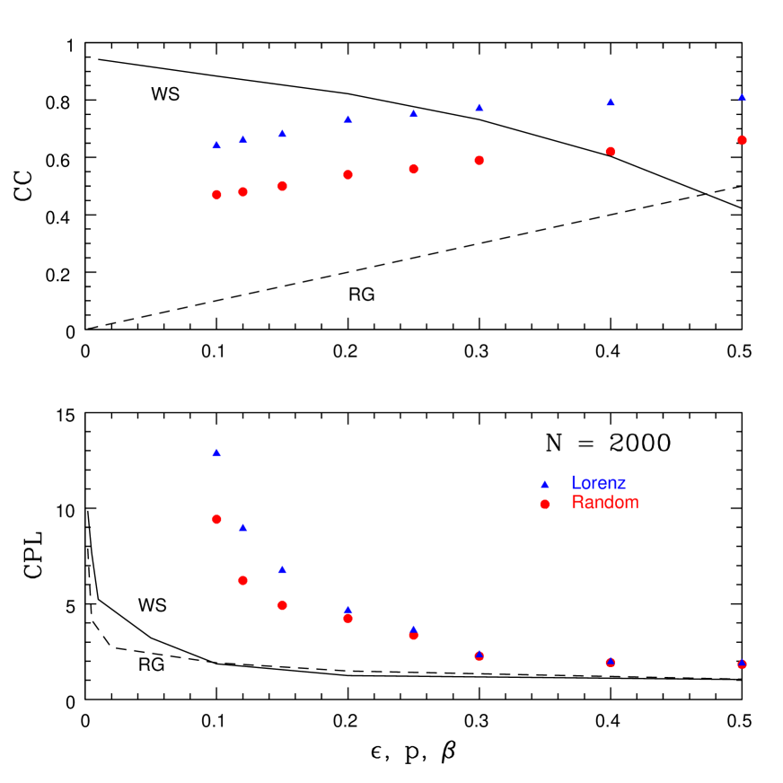
Figure 5: Variation of the CPL and CC of RNs when the recurrence threshold $\epsilon$ is increased from a value close to the percolation threshold $\epsilon=0.1$ with $M=3$. The RN first undergoes a smooth transition to a network with high CC ($\sim 0.8$) and small CPL ($<5$), capable of showing SW property for an intermediate range of $\epsilon$ approximately between $0.25$ and $0.5$. As $\epsilon\rightarrow 1$, the RN is found to cross over to the classical RG (in the limit $p\rightarrow 1)$, where both CC and CPL $\rightarrow 1$ independent of $N$. We also show the variation of CC and CPL for a W-S network as a function of the re-wiring probability $\beta$ (solid line) and the same for a RG with connection probability $p$ (dashed line). The number of nodes in all cases is $2000$.

The results of our computations are shown in Fig. 3 using a combined CPL-CC graph for $N=2000$ in all cases except the W-S network. We have shown the values for the RN of a random time series and those from $3$ different SF networks, RGs and W-S small-world networks. The values for a RGG in $3$ dimensions with the range limited to that of the RN (in $3$ dimensions) are also shown. Two results are evident from the figure. The CPL values of all networks except the RN and RGG are very small and always $<6$. Secondly, the RG with $p=0.0035$, whose degree distribution coincides with that of the RN from the random time series behaves completely differently in the CPL-CC graph. The reason for this discrepancy is the absence of long range connections in the RN. In fact, this is true for all RNs and this property cannot change with the increase in the number of nodes $N$. Both CPL and CC are found to converge and saturate to a finite value for all RNs and cannot fall below a certain limiting value which depends on $\epsilon$. This limiting value is much higher compared to the typical values for SF networks and RGs. This is shown in Fig. 4 using RNs constructed from several standard chaotic attractors with $N$ varying from $1000$ to $10000$. Our numerical results show that RNs, constructed with $\epsilon$ within the usual operational window, cannot show SW property.

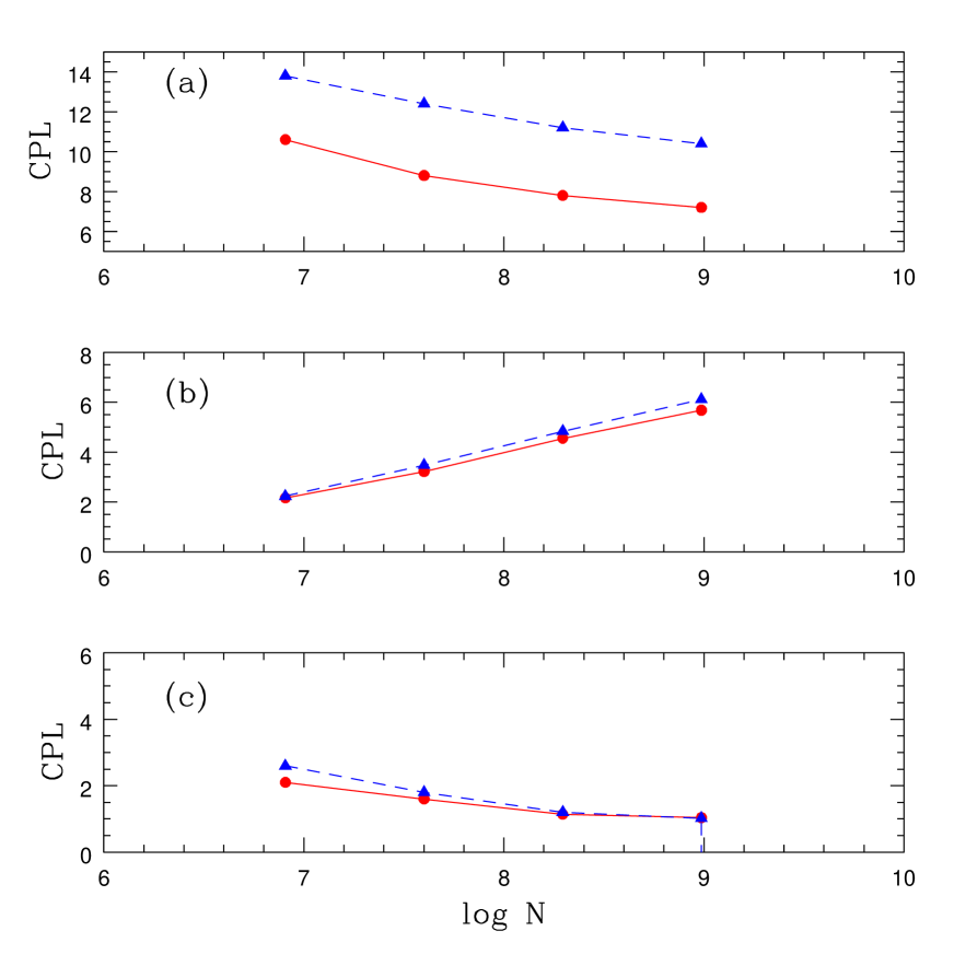
Figure 6: Variation of CPL as a function of $log$ $N$ for RNs corresponding to the $3$ ranges of threshold $\epsilon$ used for the construction of the network. The top panel (a) corresponds to $\epsilon$ within the range of recurrence thresholds where the RN represents the characteristic properties of the attractor and the CPL converges to a limiting value as $N$ increases. The middle panel (b) corresponds to intermediate values of $\epsilon$ (between $0.25$ and $0.5$) where the RN is capable of displaying the SW property as CPL increases linearly with $log$ $N$. The bottom panel (c) corresponds to large values of $\epsilon$ ($>0.5$) where the RN has long range connections and the CPL tends to a small value independent of $N$. For (b), the value of $\epsilon$ is tuned within the respective range keeping $<k>$ constant as $N$ is increased. We find the SW property for a range of $<k>$ values between $600$ to $1500$ depending on the value of $\epsilon$. The graph in (b) is plotted with $\epsilon=0.3$ and decreasing $\epsilon$ as $N$ is increased by fixing $<k>=800$. In all three cases shown above, the solid triangles connected by a dashed line represent the CPL of Lorenz attractor while the solid circles connected by a solid line represent that from random time series.

Suppose that we now increase the value of $\epsilon$ above the recurrence threshold which, in turn, increases the range of spatial connection for each node in the RN. The resulting RN may not be able to characterize the statistical properties of the embedded attractor, but one can look at the properties of the resulting network from a complex network perspective. For example, in the case of spatial networks, such as, communication and transportation networks, Barthelemy [40, 41] has shown that as the interaction range between nodes is of the order of system size or larger, the spatial effects become negligible and the networks tend to show SF property. RNs are spatially constrained networks and hence we now check whether, under some limiting conditions, the RNs can show properties of either SW networks or classical RGs.

In Fig. 5, we show the variation of CC and CPL for the RNs from random time series and Lorenz attractor as a function of $\epsilon$. While the CC shows a steady increase with $\epsilon$, the CPL decreases much more quickly initially and saturates to the minimum possible value of $1$. We also show the CC and CPL for the RG (dashed line) for increasing values of $p$ and a typical Watts-Strogatz SW network (solid line) as a function of increasing re-wiring probability $\beta$. We find that for an intermediate range of $\epsilon$ values, approximately from $0.25$ to $0.5$, the RNs show high CC ($\sim 0.8$) and small CPL ($<5$) which are the basic criteria for a network to show the small-world property. To check this, we increase the value of $N$ keeping the average degree $<k>$ approximately constant by changing the value of $\epsilon$ within the above range ( between $0.25$ and $0.5$) and compute the value of CPL as function of $log$ $N$. The result, presented in Fig. 6 (b), clearly shows the small-world property. Thus, the intermediate range of $\epsilon$ can be considered as a small-world phase for the RNs. As $\epsilon$ further increases and tends to the system size, all RNs smoothly cross over to the classical RGs with high $p$ where the CPL and CC $\rightarrow 1$ independent of $N$. To get a comparison of the behaviour between different regimes of $\epsilon$, we also show the variation of CPL with $log$ $N$ for RN with $\epsilon$ equal to the recurrence threshold in Fig. 6 (a) and for the case of long range connections with $\epsilon>0.5$ in Fig. 6 (c).

We have checked this result for two more standard chaotic attractors, namely, the Rössler attractor and the Duffing attractor and found an identical behavior. Hence, based on our numerical results, we conjecture that all RNs pass through an intermediate small-world phase as the value of $\epsilon$ is increased, before undergoing a transition to the classical RG for large $\epsilon$. Our result provides a method for constructing a SW network from time series of dynamical systems by adjusting the range of connections between the nodes. The result is also relevant to search for the SW property in network models that require a multi-dimensional system with a metric, as for example in the case of spreading of diseases [42], in continuous percolation theory [43] and in the study of random walks on fractals [44]. For example, it is well known [33] that the spreading of diseases can be modeled by a RGG. If the nature of spreading is limited to nearest neighbour interaction (say, controlled by contact only), the network cannot show SW property. However, if the spreading occurs by other means, so that the range $\epsilon$ is large, the network can very well switch over to a SW.

3 Conclusion

In this Letter, we analyse the RNs, which are unweighted and undirected graphs, from a complex network perspective. Three primary characteristics of a network, namely, the degree distribution, the CC (an averaged local measure) and the CPL (a global measure) are used for the analysis. We find that the degree distribution of every RN is unique and characteristic to the probability density variations over the representative attractor. By computing the CC and the CPL of several RNs from standard chaotic attractors, we explicitly show that the RNs constructed with the recurrence threshold at and just above the percolation threshold are basically different with both CC and CPL being high due to the absence of long range connections between the nodes.

The characteristic properties of the RN change with the value of $\epsilon$ used to construct it. As $\epsilon\rightarrow 0$, CPL $\rightarrow\infty$ and CC $\rightarrow 0$. For values of $\epsilon$ below the recurrence threshold, the RN consists of several disconnected clusters. For $\epsilon$ within the operational window above the percolation threshold, the network becomes globally connected (with the appearance of a giant component) and the RN measures characterize the statistical properties of the underlying system. In this phase, CPL remains relatively high (with the network unable show SW property) and converges to an asymptotic value as $N$ is increased.

When the value of $\epsilon$ is increased further, the constraints induced by the short connectivity range slowly disappear with the emergence of long range connections and all the RNs initially cross over to a SW phase with high CC and small CPL that increases as $log$ $N$. Finally, as the value of $\epsilon\rightarrow 1$, the RN undergoes a smooth transition to classical RGs with $p\sim 1$ with both CPL and CC $\rightarrow 1$ independent of the number of nodes N. Thus, for all RNs, there are basically three phases in terms of the range of $\epsilon$ values used for the construction of the RN, namely, a small operational window of $\epsilon$ that captures the statistical properties of the corresponding attractor, an intermediate range where the RN can display the SW property and finally $\epsilon$ of the order of the size of the attractor where the RN crosses over to the classical RG.

Acknowledgements

We thank one of the anonymous referees for several suggestions to improve our manuscript.

RJ and KPH acknowledge the financial support from Science and Engineering Research Board (SERB), Govt. of India in the form of a Research Project No SR/S2/HEP-27/2012. KPH acknowledges the computing facilities in IUCAA, Pune.

For graphical representation of networks, we use the GEPHI software:
(https://gephi.org/).

References

- [1] S. H. Strogatz, “Exploring complex networks”, Nature 410, (2001) 268–76.
- [2] M. E. J. Newman, Networks: An introduction, (Oxford University Press, New York, 2010).
- [3] B. Barzel and A. L. Barabasi, “Universality in network dynamics”, Nature Phys. 9, (2013) 673–81.
- [4] D. J. Watts, Six Degrees: The Science of a Connected Age, (Norton, New York, 2003).
- [5] S. Wasserman and K. Faust, Social Network Analysis: Methods and Applications, (Cambridge University Press, Cambridge, 1994).
- [6] M. E. J. Newman, “The structure and function of complex networks”, SIAM Rev. 45, (2003) 167–256.
- [7] S. Lawrence and C. L. Giles, “Accessibility of information on the web”, Nature 400, (1999) 107–10.
- [8] E. Bullmore and O. Sporns, “Complex brain networks: graph theoretical analysis of structural and functional systems”, Nat. Rev. Neurosci. 10, (2009) 187-98.
- [9] P. Long, D. B. Liu, S. M. Cai, L. Hong and P. L. Zhou, “Recurrence network analysis of the synchronous EEG time series in normal”, Cell Biochem. Biophys. 66, (2013) 331–38.
- [10] P. Erdős and A. Rényi, “On the evolution of random graphs”, Publ. Math. Inst. Hung. Acad. Sci. 5, (1960) 17–61.
- [11] A. L. Barabasi and R. Albert, “Emergence of scaling in random networks”, Science 286, (1999) 509–12.
- [12] R. Albert and A. L. Barabasi, “Topology of evolving networks: local events and universality”, Phys. Rev. Lett. 85, (2000) 5234–37.
- [13] M. Faloutsos, P. Faloutsos and C. Faloutsos, “On power-law relationships of the internet topology”, Comput. Commun. Rev. 29, (1999) 251–62.
- [14] M. Girvan, and M. E. J. Newman, “Community structure in social and biological networks”, Proc. Nat. Acad. Sci. USA 99, (2002) 7821–26.
- [15] R. Guimera and L. A. N. Amaral, “Functional cartography of complex metabolic networks”, Nature 433, (2005) 895–900.
- [16] R. Albert, I. Albert and G. L. Nakarado, “Structural vulnerability of the North American power grid”, Phys. Rev. E 69, (2004) 025103(R).
- [17] D. J. Watts and S. H. Strogatz, “Collective dynamics of small world networks”, Nature 393, (1998) 440–42.
- [18] H. Kantz and T. Schreiber, Nonlinear Time Series Analysis, (Cambridge University Press, Cambridge, 2004).
- [19] R. C. Hilborn, Chaos and Nonlinear Dynamics, (Oxford University Press, Oxford, 1994).
- [20] J. Zhang and M. Small, “Complex networks from pseudoperiodic time series:topology versus dynamics”, Phys. Rev. Lett. 96, (2006) 238701.
- [21] L. Lacasa, B. Luque, F. Ballesteros, J. Luque and J. C. Nuno, “From time series to complex networks: the visibility graph”, Proc. Nat. Acad. Sci. USA 105, (2008) 4972–75.
- [22] N. Marwan, J. F. Donges, Y. Zou, R. V. Donner and J. Kurths, “Complex network approach for recurrence analysis of time series”, Phys. Lett. A 373, (2009) 4246–54.
- [23] J. P. Eckmann, S. O. Kamphorst and D. Ruelle, “Recurrence plot of dynamical systems”, Europhys. Letters 5, (1987) 973–77.
- [24] P. Grassberger and I. Procaccia, “Measuring the strangeness of strange attractors”, Physica D 9, (1983) 189–208.
- [25] X. K. Xu, J. Zhang and M. Small, “Superfamily phenomena and motifs of networks induced from time series”, Proc. Nat. Acad. Sci. USA 105, (2008) 19601–05.
- [26] R. V. Donner, Y. Zou, J. F. Donges, N. Marwan and J. Kurths, “Recurrence networks: A novel paradigm for nonlinear time series analysis”, New J. Phys. 12, (2010) 033025.
- [27] R. V. Donner, M. Small, J. F. Donges, N. Marwan, Y. Zou, R. Xiang and J. Kurths, “Recurrence based time series analysis by means of complex network methods”, Int. J. Bif. Chaos 21, (2011) 1019–46.
- [28] N. Marwan and J. Kurths, “Complex network based techniques to identify extreme events and (sudden) transitions in spatio-temporal systems”, CHAOS 25, (2015) 097609.
- [29] R. Avila, A. Gapelyuk, N. Marwan, T. Walther, H. Stepan, J. Kurths and N. Wessel, “Classification of cardio-vascular time series based on different coupling structures using recurrence network analysis”, Philos. T. Roy. Soc. A 371, (2013) 20110623.
- [30] Y. Zou, J. Heitzig, R. V. Donner, J. F. Donges, J. D. Farmer, R. Meucci, S. Euzzor, N. Marwan and J. Kurths, “Power laws in recurrence networks in dynamical systems”, Europhys. Letters 98, (2012) 48001–06.
- [31] R. V. Donner, J. Heitzig, J. F. Donges, Y. Zou, N. Marwan and J. Kurths, “The geometry of chaotic dynamics-A complex network perspective”, European Phys. J. B 84, (2011) 653–72.
- [32] J. F. Donges, J. Heitzig, R. V. Donner and J. Kurths, “Analytical framework for recurrence network analysis of time series”, Phys. Rev. E 85, (2012) 046105.
- [33] J. Dall and M. Christensen, “Random geometric graphs”, Phys. Rev. E 66, (2002) 016121.
- [34] A. L. Barabasi, E. Ravasz and T. Vicsek, “Deterministic scale-free networks”, Physica A 299, (2001) 559–564.
- [35] K. P. Harikrishnan, R. Misra, G. Ambika and A. K. Kembhavi, “A non-subjective approach to the GP algorithm for analysing noisy time series”, Physica D 215, (2006) 137–145.
- [36] K. P. Harikrishnan, R. Misra and G. Ambika, “Revisiting the box counting algorithm for the correlation dimension analysis of hyperchaotic time series”, Comm. Nonlinear Sci. Num. Simulations 17, (2012) 263–276.
- [37] Fortran codes for computing and from time series can be freely downloaded from the website:
- [38] R. Jacob, K. P. Harikrishnan, R. Misra and G. Ambika, “Uniform framework for the recurrence-network analysis of chaotic time series”, Phys. Rev. E 93, (2016) 012202.
- [39] J. C. Sprott, Chaos and Time Series Analysis, (Oxford University Press, Oxford, 2003).
- [40] M. Barthelemy, “Spatial Networks”, Phys. Reports 499 (2011) 1–101.
- [41] M. Barthelemy, “Crossover from scale free to spatial networks”, Europhys. Letters 63, (2003) 915–18.
- [42] R. Pastor-Satorras and A. Vespigniani, “Epidemic spreading in scale-free networks”, Phys. Rev. Lett. 86, (2001) 3200–03.
- [43] U. Alon, A. Drory and T. Balbery, “Systematic derivation of percolation thresholds in continuum systems”, Phys. Rev. A 42, (1990) 4634–38.
- [44] P. Jund, R. Jullien and T. Campbell, “Random walks on fractals and stretched exponential relaxation”, Phys. Rev. E 63, (2001) 036131.