A deterministic global optimization using smooth diagonal auxiliary functions

Abstract

In many practical decision-making problems it happens that functions involved in optimization process are black-box with unknown analytical representations and hard to evaluate. In this paper, a global optimization problem is considered where both the goal function $f(x)$ and its gradient $f^{\prime}(x)$ are black-box functions. It is supposed that $f^{\prime}(x)$ satisfies the Lipschitz condition over the search hyperinterval with an unknown Lipschitz constant $K$. A new deterministic ‘Divide-the-Best’ algorithm based on efficient diagonal partitions and smooth auxiliary functions is proposed in its basic version, its convergence conditions are studied and numerical experiments executed on eight hundred test functions are presented.

Key Words.Global optimization, deterministic methods, Lipschitz gradients, unknown Lipschitz constant.

1 Introduction

In many important applied problems, some decisions should be made by finding the global optimum of a multiextremal objective function subject to a set of constrains (see, e. g., [9, 17, 18, 31, 32, 34, 36, 45, 46, 50, 51, 54] and the references given therein). Frequently, especially in engineering applications, the functions involved in optimization process are black-box with unknown analytical representations and hard to evaluate. Such computationally challenging decision-making problems often cannot be solved by traditional optimization techniques based on strong suppositions (such as, e. g., convexity) about the problem.

Because of significant computational costs involved, normally a limited number of functions evaluations are available for a decision-maker (physicist, biologist, economist, engineer, etc.) when he/she optimizes this kind of functions. Hence, the main goal is to construct fast global optimization algorithms that generate acceptable solutions with a relatively small number of functions evaluations.

Usually, the methods applied in this context are subdivided in stochastic and deterministic. Stochastic approaches (see, e. g., [2, 9, 18, 31, 32, 53, 54]) can often work in a simpler manner than the deterministic algorithms. They can be also suitable for the problems where the functions evaluations are corrupted by noise. However, solutions found by some stochastic algorithms (e. g., by popular heuristic methods like evolutionary algorithms, simulated annealing, etc.; see, e. g., [9, 11, 32, 38, 52]) can be only local solutions that can be located far away from the global one. This fact can preclude these methods from their usage in practice if an accurate estimate of the global solution is required. Therefore, our attention in the paper is focused on deterministic approaches.

Deterministic global optimization is an important applied field (see, e. g., [9, 18, 36, 45, 51, 55]). As a rule, deterministic methods exhibit (under certain conditions) rigorous global convergence properties and allow one to obtain guaranteed estimations of global solutions. However, deterministic models can still require too many function evaluations to achieve adequately good solutions for the considered global optimization problems.

One of the simplest techniques in this framework is represented by the so-called derivative-free (or direct) approach (see, e. g., [4, 5, 22, 30, 37]), often used for solving important applied problems (see, e. g., pattern search methods [22], the DIRECT method [20], the response surface, or surrogate model methods [21], etc.). Unfortunately (see, e. g., [6, 26, 35, 44]), these methods either are designed to detect only stationary points or can demand too high computational effort for their work. As observed, e. g., in [18, 49], if no particular assumptions are made on the objective function, any finite number of function evaluations cannot guarantee getting close to the global minimum, since the function may have very deep and narrow peaks.

The Lipschitz-continuity assumption is one of the natural suppositions on the objective function (in fact, in technical systems the energy of change is always limited). The problem involving Lipschitz functions is said to be the Lipschitz global optimization problem (see, e. g., [7, 18, 27, 36, 45, 46, 51, 54]).

The global optimization problem with a differentiable objective function having the Lipschitz gradient (with an unknown Lipschitz constant) is an important class of Lipschitz global optimization problems. Formally, this class of problems can be stated as follows:

$$f^{*}=f(x^{*})=\min_{x\in D}\;f(x),$$ (1)

$$\|f^{\prime}(x^{\prime})-f^{\prime}(x^{\prime\prime})\|\leq K\|x^{\prime}-x^{\prime\prime}\|,\hskip 8.53581ptx^{\prime},x^{\prime\prime}\in D,\hskip 8.53581pt0<K<\infty,$$ (2)

where

$$D=[a,b]=\{x\in R^{N}:a(j)\leq x(j)\leq b(j)\}.$$ (3)

It is assumed here that the objective function $f(x)$ can be black-box, multiextremal, its gradient $f^{\prime}(x)=\left(\frac{\partial f(x)}{\partial x(1)},\frac{\partial f(x)}{\partial x(2)},\ldots,\frac{\partial f(x)}{\partial x(N)}\right)^{T}$ (which can be itself an expensive multiextremal black-box vector-function) can be calculated during the search, and $f^{\prime}(x)$ is Lipschitz-continuous with some unknown constant $K$, $0<K<\infty$, over $D$. Problem (1)–(3) is frequently met in engineering (see, e. g., [36, 45, 51]), for instance, in electrical engineering design (see, e. g., [42, 51]).

There are known several methods for solving this problem that can be distinguished with respect to the way the Lipschitz constant $K$ from (3) is estimated in their computational schemes. There exist algorithms using an a priori given estimate of $K$ (see, e. g., [1, 39]), its adaptive estimates (see, e. g., [13, 14, 39]), and adaptive estimates of local Lipschitz constants (see, e. g., [39, 45]). Recently, methods working with multiple estimates of $K$ chosen from a set of possible values have been also proposed (see [25, 27]).

This paper is devoted to developing a new global optimization algorithm for solving problem (1)–(3). The new method adaptively estimates the unknown Lipschitz constant $K$ from (2) during the search and is based on efficient diagonal partitions of the search domain proposed recently. Theoretical background for the introduced method is drawn in Section 2. The algorithm is presented and analyzed theoretically in Section 3. Section 4 presents results of numerical experiments executed on several hundreds of multiextremal test functions. Finally, Section 5 concludes the paper.

2 Theoretical background

In this Section, some important theoretical results, necessary for introducing the new algorithm, are briefly described.

2.1 ‘Divide-the-Best’ algorithms

As known, many global optimization methods (of both stochastic and deterministic types) have a similar structure. Therefore, several approaches to the development of a general framework for describing global optimization algorithms and providing their convergence conditions in a unified manner have been proposed (see, e. g., [9, 16, 18, 36]). The ‘Divide-the-Best’ approach (see [40, 45]) is one of such unifying schemes. It generalizes both the schemes of adaptive partition [36] and characteristic [16, 45, 51] algorithms, which are widely used for constructing and studying global optimization methods.

Figure 1: Flow chart of ‘Divide-the-Best’ algorithms.

In a ‘Divide-the-Best’ algorithm (its generic iteration is represented by the flow chart in Figure 1), given a vector $q$ of the method parameters, an adaptive partition of the search domain $D$ from (3) into a finite set $\{D^{k}_{i}\}$ of robust subsets $D^{k}_{i}$ is considered at every iteration $k$. In Step 1, the Lipschitz constant ($K$ from (2), for the objective function gradient $f^{\prime}(x)$; or $L$ in the case of the Lipschitz objective function $f(x)$) is estimated in some way. Basing on the previously obtained information $X^{k}$, $Z^{k}$ about the objective function, the ‘merit’ (called characteristic) $R_{i}$ of each subset (see Step 2 in Figure 1) is estimated for performing a further, more detailed, investigation (see Steps 3 and 4 in Figure 1). The best (in a predefined sense) characteristic achieved over a hyperinterval $D^{k}_{t}$ corresponds to a higher possibility to determine the global minimum point within $D^{k}_{t}$ (see Step 3). The hyperinterval $D^{k}_{t}$ is then partitioned at the next iteration of the algorithm. More than one ‘promising’ hyperintervals can be subdivided at each iteration.

Various techniques (for instance, in the context of the geometric approach, see, e. g., [18, 27, 46, 51]) for selection of hyperintervals to be partitioned (see Step 3 in Figure 1) and for executing this partitioning (by means of an operator $P$, see Step 4 in Figure 1 and the following subsection 2.2) can be used within this scheme.

As the stopping criteria, one can check, e. g., the volume of a hyperinterval with the best characteristic or depletion of computational resources such as the maximal number of trials (i. e., evaluations of the objective function and its gradient).

Theoretical analysis of the ‘Divide-the-Best’ algorithms with different types of characteristics and partition operators is performed in [40, 45]. A particular attention is given there to situations (important in applied problems) when conditions of global (local) convergence are satisfied not in the whole domain $D$, but only in its small subregion(s). This can happen, e. g., in many Lipschitz global optimization algorithms that either underestimate the Lipschitz constant during their work or use local information in various subregions of $D$ (see, e. g., [23, 40, 45, 51]). It should be also noticed that the ‘Divide-the-Best’ scheme can be successfully applied to develop parallel multidimensional global optimization methods (see, e. g., [16, 51]).

2.2 Efficient partition strategy

Regarding the partition strategies (see partitioning operator $P$ on Step 4 in Figure 1), the diagonal partition strategies (see the references in [36, 44, 45, 46]) are taken into account in this paper, although other types of subdivisions are worth to be considered (see, e. g., simplicial partitions in [3, 33, 34]). In the diagonal approach, the hyperinterval $D$ from (3) is subdivided into a set of smaller hyperintervals, the objective function (and its gradient) is (are) evaluated only at two vertices corresponding to the main diagonal of the generated hyperintervals (see, e. g., vertices $a_{i}$ and $b_{i}$ of a hyperinterval $D_{i}$ in Figure 2), and the results of these trials are used to choose a hyperinterval for subsequent subdivisions. This approach has a number of interesting theoretical properties and has proved to be efficient in solving practical problems.

First, efficient one-dimensional global optimization algorithms can be easily extended to the multidimensional case by means of the diagonal approach (see, e. g., [44, 45, 46]). For instance, in order to obtain the characteristic $R_{i}$ of a multidimensional hyperinterval $D_{i}$, some univariate characteristics can be used as prototypes. After an appropriate transformation they can be considered along the one-dimensional segment being the main diagonal $[a_{i},b_{i}]$ of the hyperinterval $D_{i}$ (see smooth auxiliary function $\phi_{i}(\lambda)$ in Figure 2).

Second, the diagonal approach is computationally close to one of the simplest strategies—center-sampling technique (see, e. g., [4, 7, 8, 10, 20])—but at the same time, the function trials are executed at two points of each hyperinterval, providing so more information about the function over the subregion under investigation than center-sampling algorithms that evaluate $f(x)$ (and $f^{\prime}(x)$) only at one central point.

Figure 2: Obtaining the lower bound $R_{i}$ for the objective function $f(x)$ with the Lipschitz gradient over $D_{i}=[a_{i},b_{i}]$ by using smooth auxiliary function $\phi_{i}(\lambda)$, $\lambda\in[a_{i},b_{i}]$, along the main diagonal $[a_{i},b_{i}]$ of $D_{i}$.

An important issue in the framework of diagonal algorithms is the way the hyperintervals are partitioned during the search. Various exploration techniques based on different diagonal partition strategies are studied, e. g., in [41, 45, 46]. It is shown that partition strategies traditionally used in diagonal methods can perform many redundant trials and, hence, do not fulfil the requirements of computational efficiency (this redundancy significantly slows down the search in the case of expensive functions).

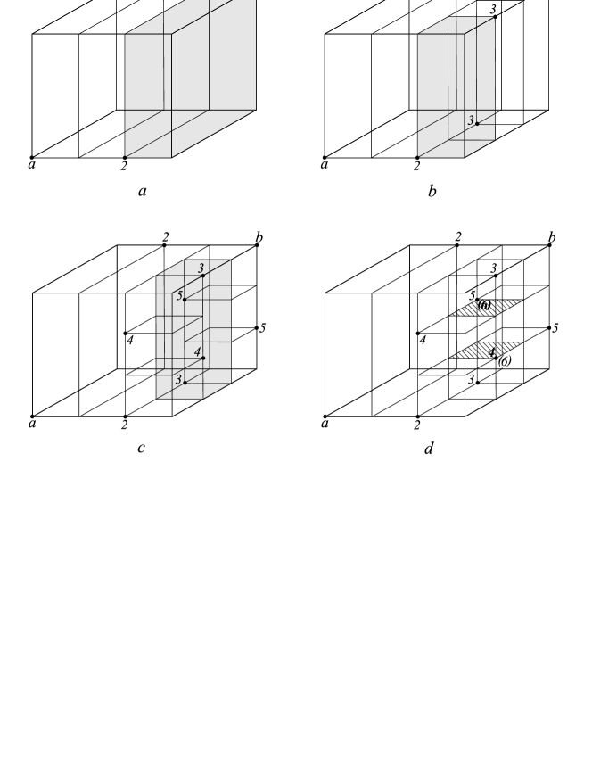
Figure 3: Example of partitioning a three-dimensional hyperinterval by the efficient diagonal partition strategy.

A diagonal partition strategy introduced in [41, 45] allows one to avoid the computational redundancy of diagonal methods. In contrast to traditional diagonal schemes, the proposed strategy (called non-redundant, or efficient diagonal partition strategy) produces regular trial meshes in such a way that one vertex where $f(x)$ and $f^{\prime}(x)$ are evaluated can belong to several hyperintervals (up to $2^{N}$, $N$ is the problem dimension from (3); see Figure 3 that shows how partitions of gray-colored hyperintervals are executed in the course of iterations 1–6, where trial points are represented by black dots). So, the time-consuming operation of evaluating both $f(x)$ and $f^{\prime}(x)$ is replaced by a significantly faster procedure of reading (up to $2^{N}$ times) the previously obtained functions values, saved in a special database (see, e. g., [45]). In Figure 3, during the 6-th iteration the partition has been performed for free since the required values of $f(x)$ and $f^{\prime}(x)$ have been already obtained at the 4-th and 5-th iterations (trial points of the 6-th iteration are in brackets, see Figure 3d). Hence, the non-redundant partition strategy speeds up the search and also leads to saving computer memory. It is important that this feature becomes more pronounced when the problem dimension $N$ increases (see, e. g., [24, 44, 45]). A formal procedure of subdivisions by means of the efficient diagonal partition strategy can be viewed in the next Section (see formulae (12)–(18)).

A novel scheme for developing fast Lipschitz global optimization methods can be, thus, considered. It can rely on the non-redundant diagonal partition strategy allowing an efficient extension of well-studied one-dimensional Lipschitz global optimization algorithms to the multidimensional case. Interesting multidimensional diagonal methods, based on different ways for achieving the Lipschitz information and constructed in the framework of the efficient diagonal approach, have been proposed and their convergence properties have been studied, e. g., in [24, 44, 45]. In the following Section, this scheme is used (see [45]) to develop a new global optimization algorithm for solving problem (1)–(3). This algorithm uses smooth diagonal auxiliary functions along the main diagonals of hyperintervals and shows how the unknown constant $K$ from (2) can be adaptively estimated during the search.

3 New algorithm SmoothD

In this Section, a new algorithm SmoothD for solving problem (1)–(3) is described. It generalizes the one-dimensional method adaptively estimating the constant $K$ (see [39]) to the multidimensional case by using the diagonal approach and the efficient partition strategy from [41, 45]. First, the new method is presented and its computational scheme is given, then its convergence properties are analyzed.

To describe the algorithm SmoothD formally, we need the following designations:

$k\geq 1$ – the current iteration number of the algorithm;

$p(k)$ – the total number of function trials executed during the previous $k-1$ iterations of the method;

$\{x^{p(k)}\}$ – the sequence of trial points generated by the algorithm in $k$ iterations;

$\{z^{p(k)}\}=\{f(x^{p(k)})\}$ – the corresponding sequence of the objective function values;

$\{\frac{\partial z^{p(k)}}{\partial x(j)}\}=\{\frac{\partial f(x^{p(k)})}{\partial x(j)}\}$, $1\leq j\leq N$, – $N$ sequences of the corresponding partial derivatives $f^{\prime}_{j}(x)$, $1\leq j\leq N$, evaluated at $x^{p(k)}$;

$M=M(k)$ – the total number of hyperintervals of the current partition of the search domain at the beginning of the $k$-th iteration;

$\{D^{k}\}=\{D_{i}^{k}\}=\{D_{i}\}$, $1\leq i\leq M$, – the current partition of the initial hyperinterval $D$ into hyperintervals $D_{i}=[a_{i},b_{i}]$.

For each hyperinterval $D_{i}$ the coordinates of the vertices $a_{i}$ and $b_{i}$ of its main diagonal $[a_{i},b_{i}]$, the corresponding values of $f(a_{i})$ and $f(b_{i})$, and the corresponding values of partial derivatives $f^{\prime}_{j}(a_{i})$ and $f^{\prime}_{j}(b_{i})$, $1\leq j\leq N$, are stored.

Directional derivatives along main diagonals are then evaluated as follows:

$$f^{\prime}(a_{i})=\left(\sum_{j=1}^{N}f^{\prime}_{j}(a_{i})(b_{i}(j)-a_{i}(j))\right)/\Delta_{i},$$ (4)

$$f^{\prime}(b_{i})=\left(\sum_{j=1}^{N}f^{\prime}_{j}(b_{i})(b_{i}(j)-a_{i}(j))\right)/\Delta_{i},$$ (5)

where

$$\Delta_{i}=\|a_{i}-b_{i}\|=\sqrt{\sum_{j=1}^{N}(a_{i}(j)-b_{i}(j))^{2}}$$ (6)

is the length of the main diagonal of hyperinterval $D_{i}$, $1\leq i\leq M(k)$.

New Algorithm SmoothD. Set the initial value of the iteration counter $k:=1$. Evaluate the objective function $f(x)$ and its partial derivatives $f^{\prime}_{j}(x)$, $1\leq j\leq N$, at the vertices $a$ and $b$ of the search domain $D$: $x^{1}=a$, $x^{2}=b$. Set both the current number of trials $p(1):=2$ and the current number of hyperintervals $M(1):=1$. The initial partition of the search domain is $\{D^{1}\}:=\{D\}$.

Suppose that $k\geq 1$ iteration of the algorithm have been already executed. Iteration $k+1$ consists of the following Steps.

Step 1 (Estimation of the Lipschitz constant for the gradient). Obtain the current estimate $m$ of the Lipschitz constant $K$ from (2) for the objective function gradient as

$$m=r\max\{\xi,\hat{m}\},$$ (7)

where $r>1$ is the reliability parameter of the method, $\xi$ is a small positive value (it ensures the correct algorithm execution when the value $\hat{m}$ is too small; as a rule, $\xi\leq 10^{-6}$), and $\hat{m}$ is found as

$$\hat{m}=\max_{1\leq i\leq M(k)}\{w_{i}\},$$

with

$$w_{i}=\frac{|2(f(a_{i})-f(b_{i}))+(f^{\prime}(a_{i})+f^{\prime}(b_{i}))\Delta_{i}|+d_{i}}{\Delta_{i}^{2}}$$

and

$$d_{i}=\{[2(f(a_{i})-f(b_{i}))+(f^{\prime}(a_{i})+f^{\prime}(b_{i}))\Delta_{i}]^{2}\,+\\ +\,(f^{\prime}(b_{i})-f^{\prime}(a_{i}))^{2}\Delta_{i}^{2}\}^{\frac{1}{2}}.$$

Step 2 (Characteristics calculations). For each hyperinterval $D_{i}\in\{D^{k}\}$, $1\leq i\leq M(k)$, calculate its characteristic $R_{i}$, being the minimum of the auxiliary function $\phi_{i}(\lambda)$ on the diagonal $[a_{i},b_{i}]$ (see Fig. 2), as follows.

Step 2.1. If inequality

$$\pi^{\prime}_{i}(y_{i})\pi^{\prime}_{i}(y^{\prime}_{i})<0,$$

is verified, where $\pi^{\prime}_{i}(y_{i})$, $\pi^{\prime}_{i}(y^{\prime}_{i})$ are found by formulae

$$\pi^{\prime}_{i}(y_{i})=my_{i}+B_{i},\hskip 14.22636pt\pi^{\prime}_{i}(y^{\prime}_{i})=my^{\prime}_{i}+B_{i},$$

with

$${\displaystyle y_{i}=\frac{\Delta_{i}}{4}+\frac{f^{\prime}(b_{i})-f^{\prime}(a_{i})}{4m}\,+}\\ {\displaystyle+\,\frac{f(a_{i})-f(b_{i})+f^{\prime}(b_{i})\Delta_{i}+0.5m\Delta_{i}^{2}}{m\Delta_{i}+f^{\prime}(b_{i})-f^{\prime}(a_{i})},}$$

$${\displaystyle y_{i}^{\prime}=-\frac{\Delta_{i}}{4}-\frac{f^{\prime}(b_{i})-f^{\prime}(a_{i})}{4m}\,+}\\ {\displaystyle+\,\frac{f(a_{i})-f(b_{i})+f^{\prime}(b_{i})\Delta_{i}+0.5m\Delta_{i}^{2}}{m\Delta_{i}+f^{\prime}(b_{i})-f^{\prime}(a_{i})},}$$

$$B_{i}=f^{\prime}(b_{i})-2my_{i}+m\Delta_{i},$$

then go to Step 2.2. Otherwise, go to Step 2.3.

Step 2.2. Calculate characteristic $R_{i}$ as

$$R_{i}=\min\{f(a_{i}),\phi_{i}(\hat{x_{i}}),f(b_{i})\},$$ (8)

where

$$\phi_{i}(\hat{x_{i}})=f(b_{i})-f^{\prime}(b_{i})\Delta_{i}-0.5m\Delta_{i}^{2}+my_{i}^{2}-0.5m\hat{x_{i}}^{2}$$

and

$$\hat{x_{i}}=2y_{i}-m^{-1}f^{\prime}(b_{i})-\Delta_{i}.$$

Go to Step 3.

Step 2.3. Calculate characteristic $R_{i}$ as

$$R_{i}=\min\{f(a_{i}),f(b_{i})\}.$$ (9)

Step 3 (Hyperinterval selection). Select a hyperinterval $D_{t}\in\{D^{k}\}$ for the further partitioning such that condition

$$t=\arg\min_{1\leq i\leq M(k)}{R_{i}}$$ (10)

is verified. If there are several hyperintervals satisfying condition (10), then choose among them the hyperinterval with the minimal index $t$.

Step 4 (Stopping criterion). If

$$\|a_{t}-b_{t}\|\leq\varepsilon\|a-b\|,$$ (11)

where $\varepsilon>0$ is a given accuracy, then stop the algorithm.

Take as an estimate of the global minimum $f^{*}$ value $z_{k}^{*}$

$$z^{*}_{k}=\min\{z\mid z\in z^{p(k)}\},$$

attained at point

$$x^{*}_{k}={\rm arg}\min_{x^{i}\in x^{p(k)}}f(x^{i}).$$

Otherwise, go to Step 5.

Step 5 (Generation of points $u$ and $v$). Calculate coordiantes of points $u$ and $v$ for partitioning the hyperinterval $D_{t}=[a^{k}_{t},b^{k}_{t}]$:

$$u=(a(1),\ldots,a(i-1),a(i)\,+\\ +\,\frac{2}{3}(b(i)-a(i)),a(i+1),\ldots,a(N)),$$ (12)

$$v=(b(1),\ldots,b({i-1}),b(i)+\,\\ +\frac{2}{3}(a(i)-b(i)),b(i+1),\ldots,b(N)),$$ (13)

where $a(j)=a^{k}_{t}(j),\ b(j)=b^{k}_{t}(j),\ 1\leq j\leq N$, and $i$ is found as

$$i=\min\,\arg\max_{1\leq j\leq N}\{|b(j)-a(j)|\}.$$ (14)

Check whether the function $f(x)$ and its partial derivatives $f_{j}^{\prime}(x)$, $1\leq j\leq N,$ have been already evaluated at the points $u$ and $v$.

Step 5.1. If $f(x)$ and $f_{j}^{\prime}(x)$, $1\leq j\leq N$, have been previously evaluated at both the points $u$ and $v$, then set $p(k+1):=p(k)$ and go to Step 6.

Step 5.2. If $f(x)$ and $f_{j}^{\prime}(x)$, $1\leq j\leq N$, have been previously evaluated at only one point, e. g., at point $u$ (similar operation is performed in the case when the functions evaluations have been performed only at point $v$), then perform a new trial of $f(x)$ and $f_{j}^{\prime}(x)$, $1\leq j\leq N$, at point

$$x^{p(k)+1}=v\,,$$

set $p(k+1):=p(k)+1$ and go to Step 6.

Step 5.3. If neither $f(x)$ nor $f_{j}^{\prime}(x)$, $1\leq j\leq N$, have been previously evaluated at points $u,\,v$, then evaluate $f(x)$ and $f_{j}^{\prime}(x)$, $1\leq j\leq N$, at points

$$x^{p(k)+1}=u,\ \ x^{p(k)+2}=v,$$

set $p(k+1):=p(k)+2$ and go to Step 6.

Step 6 (Efficient diagonal partition). Obtain a new partition $\{D^{k+1}\}$ of the search domain $D$:

$${\displaystyle\{D^{k+1}\}=\{D^{k}\}\setminus\{D_{t}\}\cup\{D^{k+1}_{M(k)+1}\}\cup\{D^{k+1}_{M(k)+2}\},}$$ (15)

where vertexes of the main diagonals of new hyperintervals $D^{k+1}_{t}$, $D^{k+1}_{M(k)+1}$ and $D^{k+1}_{M(k)+2}$ are given by formulae

$$a^{k+1}_{t}=a_{M(k)+2}=u,\hskip 5.69054ptb^{k+1}_{t}=b_{M(k)+1}=v.$$ (16)

$$a_{M(k)+1}=a^{k}_{t},\hskip 5.69054ptb_{M(k)+1}=v,$$ (17)

$$a_{M(k)+2}=u,\hskip 5.69054ptb_{M(k)+2}=b^{k}_{t},$$ (18)

respectively.

Set $M(k+1):=M(k)+2$, increase the iteration counter $k:=k+1$ and go to Step 1.

The introduced algorithm SmoothD belongs to the class of diagonally extended geometric algorithms and, thus, to a more general class of ‘Divide-the-Best’ algorithms (see [40]). Its reliability parameter $r$ from (7) controls the estimate $m$ of the Lipschitz constant $K$ of $f^{\prime}(x)$ and affects the algorithm’s convergence, as it will be shown in the next Section. Namely, by increasing $r$ the reliability of the method also increases. As this parameter decreases, the search rate increases, but the probability of convergence to a point other than the global minimizer of $f(x)$ grows as well.

The next Theorem establishes convergence properties of the proposed algorithm.

Theorem 1

For any function $f(x)$ with the gradient satisfying the Lipschitz condition $(\ref{LGOP_K})$ with the constant $K,\,\,0<K<\infty,$ there exists a value $r^{*}$ of the reliability parameter $r$ of the SmoothD algorithm such that for any $r\geq r^{*}$ the infinite ($\varepsilon=0$ in (11)) sequence of trial points $\{x^{p(k)}\},$ generated by the SmoothD algorithm during minimization of $f(x),$ will converge only to the global minimizers of $f(x)$.

Proof. This result can be obtained as a particular case of the general convergence study of ‘Divide-the-Best’ algorithms from [40] and its proof is so omitted. $\hfill\Box$

It should be noticed in this context that if a value of $r$ smaller than $r^{*}$ is used, the algorithm can converge (see the general analysis executed for ‘Divide-the-Best’ methods in [40]) to a local minimizer of $f(x)$ or to the boundary of a subregion of $D$ corresponding to the best characteristics (8)–(10). This situation indicates the necessity to increase the value of the reliability parameter, i. e., it is a practical hint for the choice of $r$.

4 Numerical experiments

In this Section, results of numerical experiments aimed at evaluating the SmoothD method performance and comparing it with some known global optimization techniques are given. Particularly, two popular global optimization algorithms (downloadable from http://www4.ncsu.edu/~ctk/SOFTWARE/DIRECTv204.tar.gz) have been taken for numerical comparisons: the DIRECT method from [20] and its locally-biased version DIRECTl from [10]. Both of them partition the search region $D$ into small hyperintervals and are widely used for solving applied black-box global optimization problems, being therefore important competitors for the SmoothD method. They also belong to the class of ‘Divide-the-Best’ algorithms but do not use the information about the objective function gradient during their work.

All experiments were performed on a 3.40 GHz Intel(R) Core(TM) i7-2600 CPU PC with 12 Gb memory using 64-bit Windows system.

This Section is structured as follows. First, methodology of executing numerical experimentation is described presenting test functions and comparison criteria used. Then, numerical issues on the reliability parameter of the new method are discussed and sensitivity analysis of this parameter is performed. Finally, overall numerical results are summarized and commented on.

4.1 Classes of test functions and comparison criteria

Eight classes of differentiable test problems generated by the GKLS-generator from [12] were used to perform numerical experiments. This generator constructs three types (non-differentiable, continuously differentiable, and twice continuously differentiable) of classes of multidimensional and multiextremal test functions with known local and global minima. The generation procedure consists of defining a convex quadratic function systematically distorted by polynomials.

Each test class provided by the generator consists of 100 functions and is defined by the following parameters: (i) problem dimension $N$, (ii) number of local minima $m$, (iii) global minimum value $f^{*}$, (iv) radius of the attraction region of the global minimizer $\rho$, (v) distance from the global minimizer to the quadratic function vertex $d$. The other necessary parameters are chosen randomly by the generator for each test function of the class. A special notebook with a complete description of all functions is supplied to the user. The GKLS-generator always produces the same test classes for a given set of the user-defined parameters, allowing one to perform repeatable numerical experiments. By changing the user-defined parameters, classes with different properties can be created. The generator is available on the ACM Collected Algorithms (CALGO) database (the CALGO is part of a family of publications produced by the Association for Computing Machinery) and it is also downloadable for free from http://wwwinfo.dimes.unical.it/~yaro/GKLS.html.

In order to obtain comparable results, the same eight GKLS test classes of continuously differentiable functions of dimensions $N=2,3,4$, and 5 defined by the same five parameters as in [44] were used (see Table 1). The global minimum value $f^{*}$ was equal to $-1.0$ and the number of local minima $m$ was equal to 10 for all classes (these values are default settings of the GKLS-generator). Two test classes were considered for each particular dimension $N$: the ‘simple’ class and the ‘hard’ one. The difficulty of a class was increased either by decreasing the radius $\rho$ of the attraction region of the global minimizer $x^{*}$ (as for two- and five-dimensional classes) or by increasing the distance $d$ from $x^{*}$ to the quadratic function vertex (three- and four-dimensional classes).

Table 1: Description of the GKLS test classes used in numerical experiments

Class	Difficulty	$\varepsilon$	$N$	$m$	$f^{*}$	$d$	$\rho$
1.	Simple	$10^{-4}$	2	10	$-1.0$	0.90	0.20
2.	Hard	$10^{-4}$	2	10	$-1.0$	0.90	0.10
3.	Simple	$10^{-6}$	3	10	$-1.0$	0.66	0.20
4.	Hard	$10^{-6}$	3	10	$-1.0$	0.90	0.20
5.	Simple	$10^{-6}$	4	10	$-1.0$	0.66	0.20
6.	Hard	$10^{-6}$	4	10	$-1.0$	0.90	0.20
7.	Simple	$10^{-7}$	5	10	$-1.0$	0.66	0.30
8.	Hard	$10^{-7}$	5	10	$-1.0$	0.66	0.20

In all numerical experiments, the maximal allowed number of function trials was set equal to $p_{max}=1\,000\,000$. A problem was considered to be solved by a method under examination if the method generated a trial point $x^{\prime}$ in an $\varepsilon$-neighborhood of the global minimizer $x^{*}\in D=[a,b]$, i. e.,

$$|x^{\prime}(j)-x^{*}(j)|\leq\sqrt[n]{\varepsilon}(a(j)-b(j)),\quad 1\leq j\leq N,$$ (19)

where $0<\varepsilon<1$ is an accuracy coefficient (its values are given in the third column of Table 1). Such a type of stopping criterion is acceptable only when the global minimizer $x^{*}$ is known, i. e., in the case of test functions. When a real black-box objective function is minimized and global minimization methods have an internal stopping criterion (as that of the proposed algorithm, see formula (11)), they execute a number of iterations (that can be high) after a ‘good’ estimate of $f^{*}$ has been achieved in order to demonstrate the ‘goodness’ of the solution found (see, e. g., [18, 36, 51]).

Since each evaluation of a real-life black-box objective function is usually a time-consuming operation (see, e. g., [19, 34, 36, 45, 48, 51, 54]), the maximal number of function trials executed by the methods until the satisfaction of the stopping criteria (19) was chosen as the main criterion of the comparison (other possible comparison indicators as the number of generated hyperintervals, the average number of trials, and so on can be also used, see, e. g., [33, 44, 45, 48]).

4.2 The reliability parameter and its sensitivity analysis

In order to evaluate the influence of the reliability parameter $r$ from (7) on the convergence properties of the SmoothD method, the two-dimensional class 1 from Table 1 was taken. A problem from this class was considered to be solved by the new method if it generated a trial satisfying condition (19) (if the method stopped due to its internal stopping criterion (11) and condition (19) was not verified, the problem was considered to be unsolved by SmoothD with a given value of the reliability parameter).

The following numbers were taken as indicators of the SmoothD method performance in this analysis subject to a fixed value $\bar{r}$ of the reliability parameter $r$, equal to all 100 functions of the class:

$S(\bar{r})$ – number of solved problems among 100 of the test class;

$p^{*}(\bar{r})$ – maximal number of trials required for the method to satisfy condition (19) for all $S(\bar{r})$ functions of the test class;

$p_{\rm avg}(\bar{r})$ – average number of trials required for the method to satisfy condition (19) for all $S(\bar{r})$ functions of the test class.

Numerical results obtained by the proposed method on the considered two-dimensional test class when the reliability parameter varied from $\bar{r}=1.2$ up to $\bar{r}=5.8$ are reported in Table 2.

Table 2: Influence of the reliability parameter on the SmoothD method performance in the case of the two-dimensional GKLS test class 1

Indicator	$\bar{r}=1.2$	$\bar{r}=1.8$	$\bar{r}=2.8$	$\bar{r}=3.8$	$\bar{r}=4.8$	$\bar{r}=5.8$
$p^{*}(\bar{r})$	199	272	332	410	424	451
$p_{\rm avg}(\bar{r})$	105.14	169.63	222.16	293.52	323.42	341.60
$S(\bar{r})$	51	81	91	98	99	100

It can be seen from Table 2 that with increasing the value of $r$ the reliability (the number of solved problems $S(\bar{r})$) of the method increases. However, the numbers of trials (both maximal and average) increase too. This is due to the fact (well known in Lipschitz global optimization; see, e. g., [48]) that every function optimized by the proposed method has its own value $r^{*}$ from Theorem 1. Therefore, when one executes tests with a class of 100 different functions it becomes difficult to use specific values of $r$ for each function.

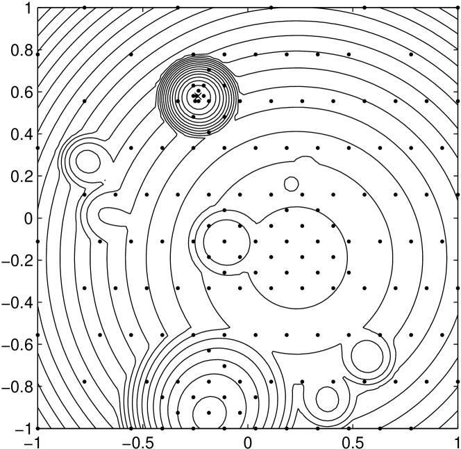
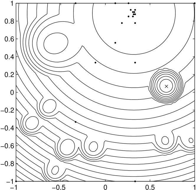
Figure 4: Trial points (black dots) generated by the SmoothD method when minimizing function number 58 from the GKLS test class 1, $x^{*}\approx(-0.2371,0.5791)$ (left: $\bar{r}=1.2$, 152 trials; right: $\bar{r}=5.8$, 452 trials).

Figure 5: Trial points (black dots) generated by the SmoothD method when minimizing function number 54 from the GKLS test class 1 , $x^{*}\approx(0.6841,0.0664)$ (left: $\bar{r}=1.2$, 20 trials; right: $\bar{r}=5.8$, 375 trials).

In fact (see an illustration given in Figures 5 and 5), for one particular function (see Figure 5, left part) a relatively small value of $r$ can be already sufficient to find its global minimizer in sense of condition (19). In this case, a higher value of the reliability parameter (see Figure 5, right part) can cause the method to perform an additional examination of the search domain in the hope of capturing an eventual better minimum. Obviously, this exploration increases the number of trials performed by the method on this particular function (see Figure 5, right part) but allows the method to solve some other problem (as that in Figure 5) for which a greater value of $r$ is required. An insufficient (i.e., too small) value of $r$ makes the method converge to a local minimizer, as it is shown in Figure 5, left part. It should be noticed in this connection that in some practical applications the discovering of a local minimizer can be also very useful. Figure 5, left part, shows that when local solutions are of an interest, the algorithm SmoothD can provide a fast convergence to local minimizers with small values of $r$.

In order to avoid an excessive exploration of the search region, several approaches can be used. For example, an adaptive adjustment of the reliability parameter can be performed using the following formula

$$r=\bar{r}+\frac{C}{k},$$ (20)

where $k$ is the iteration number of the method and $C$ is a positive constant. In this way, at the initial iterations of the method (when $k$ is small) a greater attention is paid to the exploration of the whole search domain $D$ while for high values of $k$ the influence of $C$ diminishes and the reliability parameter becomes closer to its fixed value $\bar{r}$. As it can be seen from results in Table 3 (where the same values $\bar{r}$ as in Table 2 were used but with different values $C>0$ in (20)), this adaptive technique improves the method performance.

Table 3: Analysis of the adaptive reliability parameter of the SmoothD method in the case of the two-dimensional GKLS test class 1

Indicator	$\bar{r}=1.2$	$\bar{r}=1.8$	$\bar{r}=2.8$	$\bar{r}=3.8$	$\bar{r}=4.8$	$\bar{r}=5.8$
			$C=10.0$
$p^{*}(\bar{r})$	201	277	377	410	424	453
$p_{\rm avg}(\bar{r})$	113.16	176.06	250.45	294.64	324.10	342.01
$S(\bar{r})$	62	86	96	98	99	100
			$C=20.0$
$p^{*}(\bar{r})$	179	283	379	411	424	453
$p_{\rm avg}(\bar{r})$	122.01	181.26	252.86	295.51	324.73	342.47
$S(\bar{r})$	69	86	96	99	99	100
			$C=50.0$
$p^{*}(\bar{r})$	214	293	387	414	425	454
$p_{\rm avg}(\bar{r})$	146.42	194.98	257.56	299.23	327.24	343.83
$S(\bar{r})$	83	92	100	100	100	100
			$C=100.0$
$p^{*}(\bar{r})$	251	314	369	416	428	456
$p_{\rm avg}(\bar{r})$	170.40	212.98	247.72	305.07	330.47	345.85
$S(\bar{r})$	92	97	100	100	100	100

As a practical recommendation for solving real-life global optimization problems, the following procedure can be adopted. An initial number of trials that are to be performed is fixed and the method is started with a small value of $r$. Once the method stopped, it is restarted on the same pool of trial points (without re-evaluating $f(x)$ and $f^{\prime}(x)$) but with a greater value of $r$. If after repeating these restarts several times the method converges to the same point, this point is accepted as an approximation of the global minimizer. For more information on the reliability parameter and other parameters of this kind in Lipschitz global optimization see, e. g., [48, 51].

4.3 Operating characteristics of the compared methods

The overall numerical results for three compared methods on the considered GKLS test classes are summarized in this subsection. Since the DIRECT-type methods under examination do not have any internal stopping criteria, they stopped either when condition (19) was satisfied or when $p_{max}$ trials were performed. During their work, these methods evaluate only the objective function $f(x)$ from (1) (and do not evaluate $f^{\prime}(x)$ as the SmoothD method does), therefore the operation of executing a trial is less expensive in the DIRECT-type algorithms with respect to that of the new method. The balancing parameter $\epsilon$ of the DIRECT and DIRECTl methods (see [10, 20]) was set equal to $\epsilon=10^{-4}$, as recommended by many authors (see, e.g., the review of different techniques for setting this parameter in [33]).

Formula (20) was used in the SmoothD method to set the reliability parameter $r$ from (7), with the value $\xi=10^{-6}$ in (7) and the values $C$ from (20) set in relation to the problems dimension ($C$ equal to $50$, $100$, $150$, and $200$ in the case of $N$ equal to 2, 3, 4, and 5, respectively). Moreover, several values of $\bar{r}$ can be fixed for the entire class starting from the initial value $\bar{r}=1.1$ (the maximal values of this coefficient were equal to 2.80, 5.80, 3.60, 4.30, 5.80, 6.60, 4.10, and 7.80 for the GKLS classes from 1 to 8, respectively).

The algorithms performance can be conveniently visualized by the operating characteristics (introduced in 1978 in [15], see, e. g., [51] for their English-language description). The operating characteristics are formed by the pairs $(p,S(p))$ where $p$ is the number of trials and $S(p)$ ($0\leq S(p)\leq S=100$) is the number of test problems (among a set of $S$ tests) solved by a method with less than or equal to $p$ function trials. Each pair (for increasing values of $p$) corresponds to a point on the plane. Higher is the graph of the operating characteristics of a method with respect to another one, better is the method performance on the considered set of tests.

In Figures 6 and 7, operating characteristics of the compared methods are shown, respectively, on simple and hard GKLS classes from Table 1. The numbers $p^{*}$ of trials required for the methods to satisfy condition (19) for all $100$ functions of a test class are also indicated in these Figures (after performing $p_{max}=1\,000\,000$ trials, the DIRECT method was unable to solve 4, 4, 7, 1, and 16 problems of the GKLS classes 4–8, respectively, and the DIRECTl method was unable to solve 4 problems of the GKLS class 8).

It can be seen from the graphs reported in Figures 6 and 7, that on relatively simple functions of each GKLS class (approximatively, half of 100 problems of the class quickly solved by every method) the SmoothD method behaves similarly to the DIRECT and DIRECTl methods, in terms of the function trials performed (see, e. g., the intersection of the vertical line corresponding to $p\approx 200$ trials and the operating characteristics graphs on the simple two-dimensional GKLS class 1 in Figure 6). However, when more and more difficult problems of the particular GKLS class are to be solved, the advantage of the new method becomes more and more pronounced with respect to the competitors (see the ascent of the operating characteristics graphs of the SmoothD method on all the GKLS classes in Figures 6 and 7). The most significant advantage with respect to both the DIRECT and DIRECTl methods is obtained by the new method on the hard five-dimensional GKLS class 8 (which is the most difficult among the classes from Table 1).

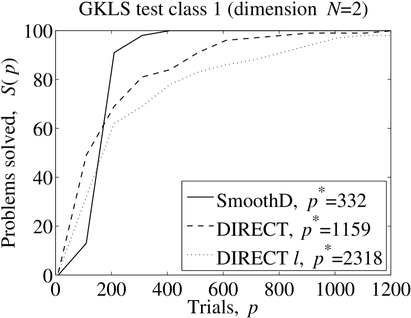
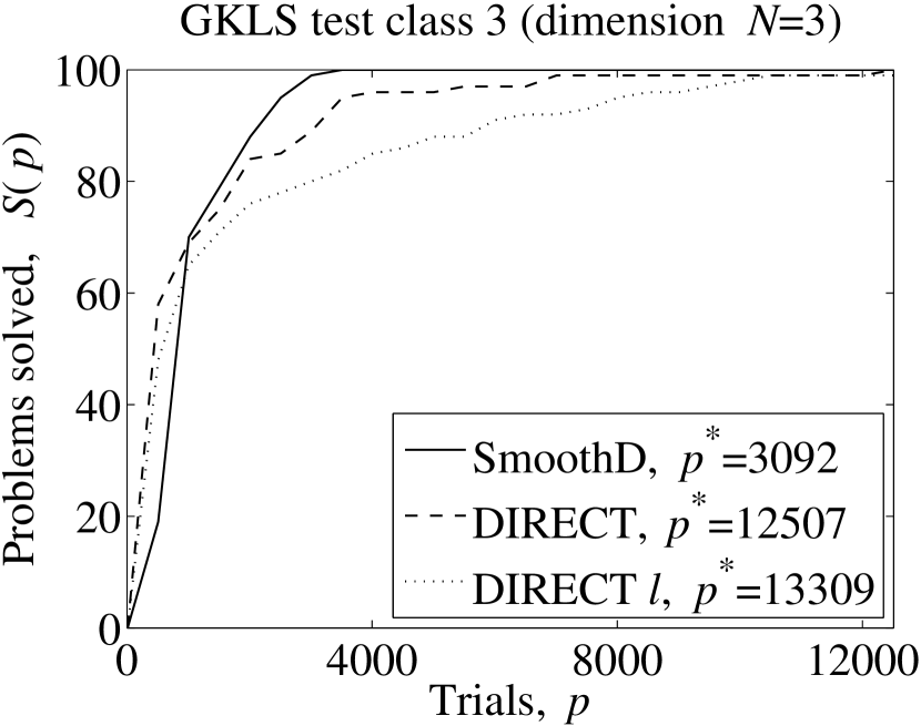
Figure 6: Operating characteristics for the compared methods SmoothD, DIRECT, and DIRECTl on ‘simple’ GKLS test classes 1, 3, 5, and 7 from Table 1.

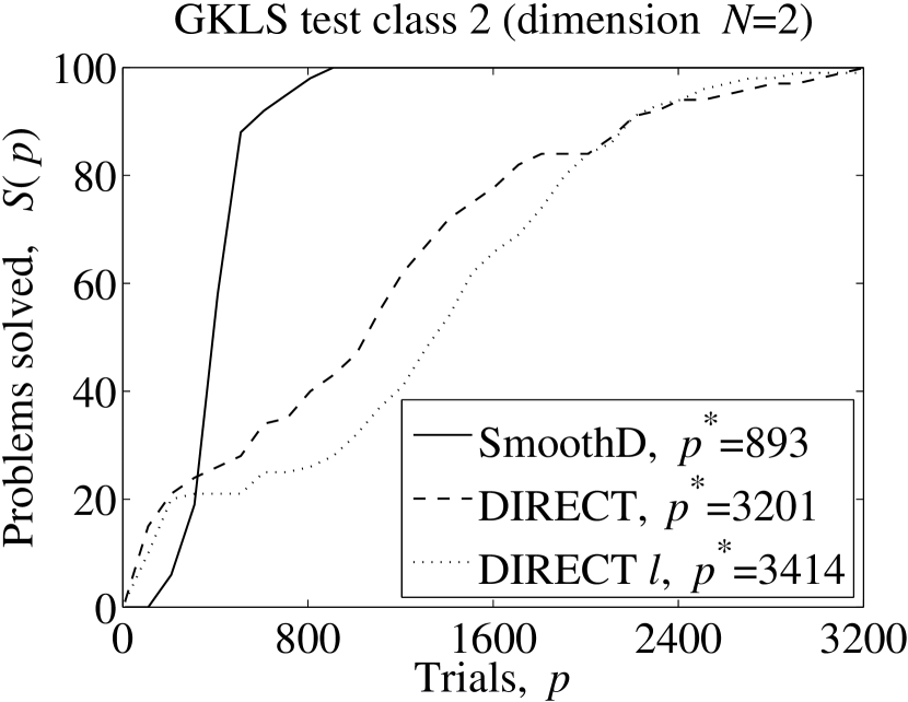
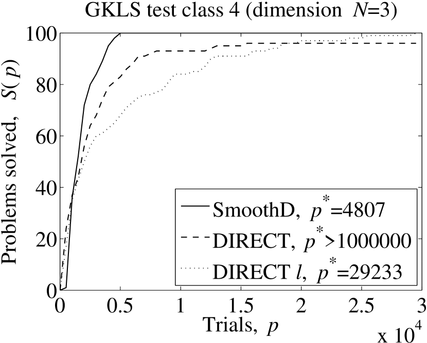
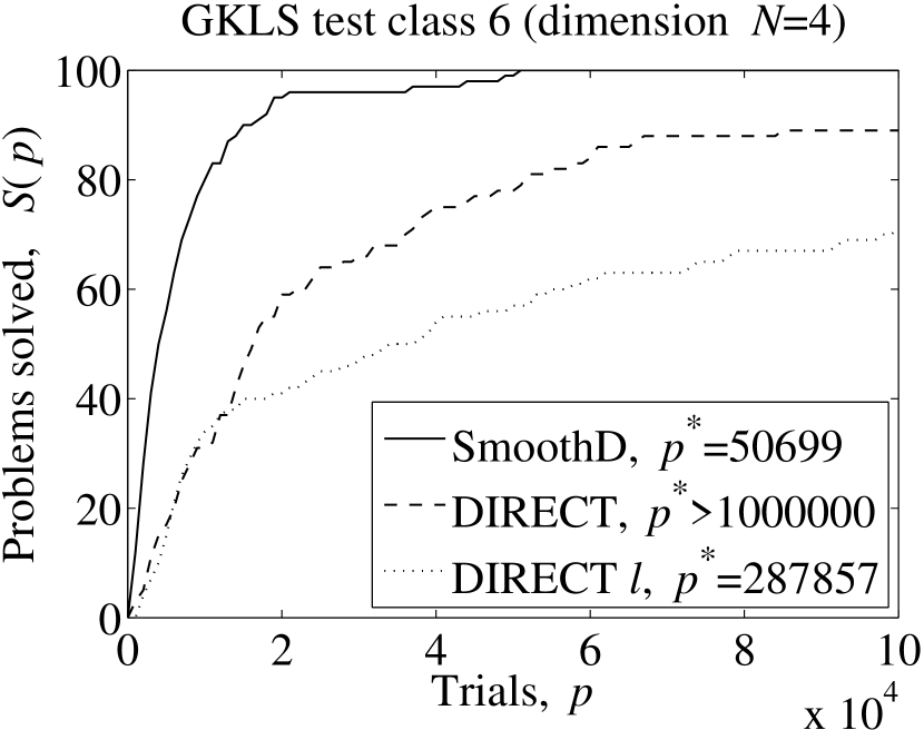
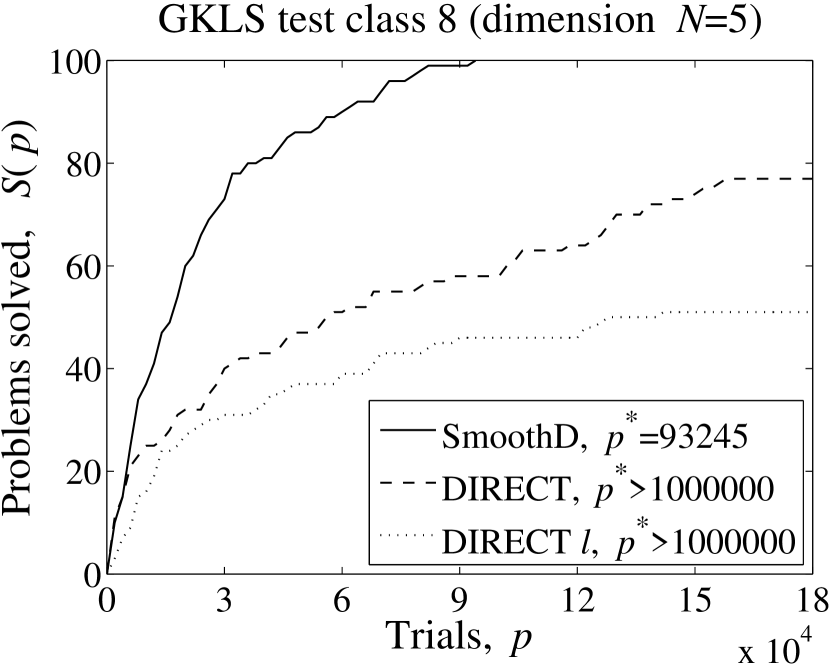
Figure 7: Operating characteristics for the compared methods SmoothD, DIRECT, and DIRECTl on ‘hard’ GKLS test classes 2, 4, 6, and 8 from Table 1.

5 A brief conclusion

A new method SmoothD has been proposed to solve global optimization problems with the objective function having the Lipschitz gradient. It generalizes the one-dimensional geometric algorithm using smooth auxiliary functions and adaptive estimate of the Lipschitz constant from [39] to the multidimensional case by using the efficient diagonal scheme from [41, 45]. The proposed method belongs to the class of ‘Divide-the-Best’ algorithms for which strong convergence properties have been established in [40]. Results of numerical experiments performed with the SmoothD method on several hundreds of GKLS test functions from [12] show that already in its basic version the proposed algorithm manifests a very nice performance and opens new directions for developing powerful global optimization tools. In the future, it could be interesting to consider, in the connection to the SmoothD method, such approaches as the local tuning [39, 45] and local improvement techniques [28, 29, 48]. Another interesting direction of research is to develop parallel versions of the proposed method within a general framework introduced in [14, 43, 47, 51] for constructing parallel global optimization techniques.

References

- [1] L. Breiman and A. Cutler. A deterministic algorithm for global optimization. Math. Program., 58(1–3):179–199, 1993.
- [2] J. M. Calvin and A. Žilinskas. One-dimensional P-algorithm with convergence rate for smooth function. J. Optim. Theory Appl., 106(2):297–307, 2000.
- [3] J. Clausen and A. Žilinskas. Subdivision, sampling, and initialization strategies for simplical branch and bound in global optimization. Comput. Math. Appl., 44(7):943–955, 2002.
- [4] A. R. Conn, K. Scheinberg, and L. N. Vicente. Introduction to Derivative-Free Optimization. SIAM, Philadelphia, USA, 2009.
- [5] A. L. Custódio, J. F. Aguilar Madeira, A. I. F. Vaz, and L. N. Vicente. Direct multisearch for multiobjective optimization. SIAM J. Optim., 21(3):1109–1140, 2011.
- [6] D. Di Serafino, G. Liuzzi, V. Piccialli, F. Riccio, and G. Toraldo. A modified DIviding RECTangles algorithm for a problem in astrophysics. J. Optim. Theory Appl., 151(1):175–190, 2011.
- [7] Yu. G. Evtushenko. Numerical Optimization Techniques. Translations Series in Mathematics and Engineering. Springer–Verlag, Berlin, 1985.
- [8] Yu. G. Evtushenko and M. A. Posypkin. An application of the nonuniform covering method to global optimization of mixed integer nonlinear problems. Comput. Math. Math. Phys., 51(8):1286–1298, 2011.
- [9] C. A. Floudas and P. M. Pardalos, editors. Encyclopedia of Optimization (6 Volumes). Springer, 2nd edition, 2009.
- [10] J. M. Gablonsky and C. T. Kelley. A locally-biased form of the DIRECT algorithm. J. Global Optim., 21(1):27–37, 2001.
- [11] A. H. Gandomi, G. J. Yun, X.-S. Yang, and S. Talatahari. Chaos-enhanced accelerated particle swarm optimization. Commun. Nonlinear Sci. Numer. Simulat., 18:327–340, 2013.
- [12] M. Gaviano, D. E. Kvasov, D. Lera, and Ya. D. Sergeyev. Algorithm 829: Software for generation of classes of test functions with known local and global minima for global optimization. ACM Trans. Math. Software, 29(4):469–480, 2003.
- [13] V. P. Gergel. A global optimization algorithm for multivariate function with Lipschitzian first derivatives. J. Global Optim., 10(3):257–281, 1997.
- [14] V. P. Gergel and Ya. D. Sergeyev. Sequential and parallel algorithms for global minimizing functions with Lipschitzian derivatives. Comput. Math. Appl., 37(4–5):163–179, 1999.
- [15] V. A. Grishagin. Operating characteristics of some global search algorithms. In Problems of Stochastic Search, volume 7, pages 198–206. Zinatne, Riga, 1978. In Russian.
- [16] V. A. Grishagin, Ya. D. Sergeyev, and R. G. Strongin. Parallel characteristic algorithms for solving problems of global optimization. J. Global Optim., 10(2):185–206, 1997.
- [17] I. E. Grossmann, editor. Global Optimization in Engineering Design. Kluwer Academic Publishers, Dordrecht, 1996.
- [18] R. Horst and P. M. Pardalos, editors. Handbook of Global Optimization, volume 1. Kluwer Academic Publishers, Dordrecht, 1995.
- [19] R. Horst and H. Tuy. Global Optimization – Deterministic Approaches. Springer–Verlag, Berlin, 1996.
- [20] D. R. Jones, C. D. Perttunen, and B. E. Stuckman. Lipschitzian optimization without the Lipschitz constant. J. Optim. Theory Appl., 79(1):157–181, 1993.
- [21] D. R. Jones, M. Schonlau, and W. J. Welch. Efficient global optimization of expensive black-box functions. J. Global Optim., 13(4):455–492, 1998.
- [22] T. G. Kolda, R. M. Lewis, and V. Torczon. Optimization by direct search: New perspectives on some classical and modern methods. SIAM Rev., 45(3):385–482, 2003.
- [23] D. E. Kvasov, C. Pizzuti, and Ya. D. Sergeyev. Local tuning and partition strategies for diagonal GO methods. Numer. Math., 94(1):93–106, 2003.
- [24] D. E. Kvasov and Ya. D. Sergeyev. Multidimensional global optimization algorithm based on adaptive diagonal curves. Comput. Math. Math. Phys., 43(1):40–56, 2003.
- [25] D. E. Kvasov and Ya. D. Sergeyev. A univariate global search working with a set of Lipschitz constants for the first derivative. Optim. Lett., 3(2):303–318, 2009.
- [26] D. E. Kvasov and Ya. D. Sergeyev. Lipschitz gradients for global optimization in a one-point-based partitioning scheme. J. Comput. Appl. Math., 236(16):4042–4054, 2012.
- [27] D. E. Kvasov and Ya. D. Sergeyev. Univariate geometric Lipschitz global optimization algorithms. Numer. Algebra Contr. Optim., 2(1):69–90, 2012.
- [28] D. Lera and Ya. D. Sergeyev. An information global minimization algorithm using the local improvement technique. J. Global Optim., 48(1):99–112, 2010.
- [29] D. Lera and Ya. D. Sergeyev. Acceleration of univariate global optimization algorithms working with Lipschitz functions and Lipschitz first derivatives. SIAM J. Optim., 23(1):508–529, 2013.
- [30] G. Liuzzi, S. Lucidi, and M. Sciandrone. Sequential penalty derivative-free methods for nonlinear constrained optimization. SIAM J. Optim., 20(5):2614–2635, 2010.
- [31] J. Mockus. A Set of Examples of Global and Discrete Optimization: Applications of Bayesian Heuristic Approach. Kluwer Academic Publishers, Dordrecht, 2000.
- [32] P. M. Pardalos and H. E. Romeijn, editors. Handbook of Global Optimization, volume 2. Kluwer Academic Publishers, Dordrecht, 2002.
- [33] R. Paulavičius, Ya. D. Sergeyev, D. E. Kvasov, and J. Žilinskas. Globally-biased disimpl algorithm for expensive global optimization. J. Global Optim., 59(2-3):545–567, 2014.
- [34] R. Paulavičius and J. Žilinskas. Simplicial Global Optimization. Springer, New York, 2014.
- [35] R. Paulavičius and J. Žilinskas. Simplicial Lipschitz optimization without the Lipschitz constant. J. Global Optim., 59(1):23–40, 2014.
- [36] J. D. Pintér. Global Optimization in Action (Continuous and Lipschitz Optimization: Algorithms, Implementations and Applications). Kluwer Academic Publishers, Dordrecht, 1996.
- [37] L. M. Rios and N. V. Sahinidis. Derivative-free optimization: A review of algorithms and comparison of software implementations. J. Global Optim., 56:1247–1293, 2013.
- [38] J. J. Schneider and S. Kirkpatrick. Stochastic Optimization. Springer, Berlin, 2006.
- [39] Ya. D. Sergeyev. Global one-dimensional optimization using smooth auxiliary functions. Math. Program., 81(1):127–146, 1998.
- [40] Ya. D. Sergeyev. On convergence of “Divide the Best” global optimization algorithms. Optimization, 44(3):303–325, 1998.
- [41] Ya. D. Sergeyev. An efficient strategy for adaptive partition of -dimensional intervals in the framework of diagonal algorithms. J. Optim. Theory Appl., 107(1):145–168, 2000.
- [42] Ya. D. Sergeyev, P. Daponte, D. Grimaldi, and A. Molinaro. Two methods for solving optimization problems arising in electronic measurements and electrical engineering. SIAM J. Optim., 10(1):1–21, 1999.
- [43] Ya. D. Sergeyev and V. A. Grishagin. A parallel method for finding the global minimum of univariate functions. J. Optim. Theory Appl., 80(3):513–536, 1994.
- [44] Ya. D. Sergeyev and D. E. Kvasov. Global search based on efficient diagonal partitions and a set of Lipschitz constants. SIAM J. Optim., 16(3):910–937, 2006.
- [45] Ya. D. Sergeyev and D. E. Kvasov. Diagonal Global Optimization Methods. FizMatLit, Moscow, 2008. In Russian.
- [46] Ya. D. Sergeyev and D. E. Kvasov. Lipschitz global optimization. In J. J. Cochran, editor, Wiley Encyclopedia of Operations Research and Management Science, volume 4, pages 2812–2828. Wiley, New York, 2011.
- [47] Ya. D. Sergeyev and R. G. Strongin. A global minimization algorithm with parallel iterations. USSR Comput. Math. Math. Phys., 29(2):7–15, 1989.
- [48] Ya. D. Sergeyev, R. G. Strongin, and D. Lera. Introduction to Global Optimization Exploiting Space-Filling Curves. Springer, New York, 2013.
- [49] C. P. Stephens and W. Baritompa. Global optimization requires global information. J. Optim. Theory Appl., 96(3):575–588, 1998.
- [50] R. G. Strongin. Numerical Methods in Multiextremal Problems (Information-Statistical Algorithms). Nauka, Moscow, 1978. In Russian.
- [51] R. G. Strongin and Ya. D. Sergeyev. Global Optimization with Non-Convex Constraints: Sequential and Parallel Algorithms. Kluwer Academic Publishers, Dordrecht, 2000.
- [52] X.-S. Yang. Engineering Optimization: An Introduction with Metaheuristic Applications. Wiley, USA, 2010.
- [53] A. A. Zhigljavsky. Theory of Global Random Search. Kluwer Academic Publishers, Dordrecht, 1991.
- [54] A. A. Zhigljavsky and A. Žilinskas. Stochastic Global Optimization. Springer, New York, 2008.
- [55] A. Žilinskas and J. Žilinskas. Interval arithmetic based optimization in nonlinear regression. Informatica, 21(1):149–158, 2010.