Ancilla assisted measurements on quantum ensembles:
General protocols and applications in NMR quantum information processing

Abstract

Quantum ensembles form easily accessible architectures for studying various phenomena in quantum physics, quantum information science, and spectroscopy. Here we review some recent protocols for measurements in quantum ensembles by utilizing ancillary systems. We also illustrate these protocols experimentally via nuclear magnetic resonance techniques. In particular, we shall review noninvasive measurements, extracting expectation values of various operators, characterizations of quantum states, and quantum processes, and finally quantum noise engineering.

I Introduction

Unlike the classical measurements, measurements in quantum physics affect the dynamics of the system. Moreover, often a particular experimental technique may offer only a limited set of observables which can be directly measured. The complete characterization of a quantum state or a quantum process requires, in general, a series of measurements of noncommuting observables - requiring repeated state preparation, and a large number independent measurements. In this article, we review recent progresses in the measurement of quantum ensembles and explain how to overcome the above challenges. Here we exploit the presence of an ancillary register interacting with the system that is to be measured. In the following section we show how to realize noninvasive measurements using ancillary qubits. Extracting expectation values of various types of operators and related applications are described in section III. We then describe an efficient protocols for complete quantum state characterization (section IV) and quantum process tomography (section V). We also narrate our experiments on noise engineering using ancillary qubits in section VI, and finally we summarize all the topics in section VII. In all the sections, we illustrate the protocols experimentally using nuclear magnetic resonance (NMR) techniques.

II Noninvasive measurements

A classical measurement can in principle be noninvasive in the sense it has no effect on the dynamics of the system. The same is not true in general for a quantum system, wherein the process of measurement itself may affect the dynamics of the system. However, as explained below, ancillary qubits can be utilized to realize certain quantum measurements without much disturbance, and hence extract probabilities or expectation values noninvasively to a great extent. Such measurements are often termed as noninvasive quantum measurements.

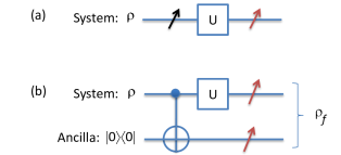
Figure 1: Circuits describing invasive and non-invasive measurements. The first measurement is invasive in (a). The same is replaced by a noninvasive measurement in (b). The final measurements are invasive in both.

Consider the example of a single qubit initialized in state $\rho$ (Fig. 1 (a)) and a dichotomic observable $Q$ with eigenvalues $q\in\{0,1\}$. Suppose we need to extract the joint probabilities $P(q_{1},q_{2})$ at two time-instances, one before applying an unitary $U$ and the other after applying $U$ (Fig. 1 (a)). To realize the first measurement noninvasively, we utilize an ancilla qubit (Fig. 1 (b)), a CNOT gate, and a final 2-qubit projective measurement in $Q\otimes Q$ basis. The CNOT operation copies the probabilities of $P(q_{1})$ onto the ancilla qubit without projecting the system state. Denoting the first qubit as the ancilla and the second qubit as the system, the diagonal elements of the joint density operator $\rho_{f}$ store the joint probabilities, i.e., $P(q_{1},q_{2})=\langle{q_{1}q_{2}}|\rho_{f}|{q_{1}q_{2}}\rangle$. The joint probabilities can thus be extracted by a final strong measurement or by a diagonal density matrix tomography Athalye et al. (2011a). Knee et al Knee et al. (2012a) argued that since CNOT operator flips the ancilla qubit if the system qubit is in state $|{1}\rangle$, the circuit is not quite noninvasive. They also proposed a simple variation, in which $P(0,0)$ and $P(0,1)$ are measured using CNOT operator, while $P(1,0)$ and $P(1,1)$ are measured using an Anti-CNOT operator (which flips the ancilla only if the system qubit is in state $|{1}\rangle$). In this procedure, called ideal negative-result measurement (INRM), all the joint probabilities are measured without flipping the ancilla qubit, and therefore is considered more noninvasive. In the following we describe the application of INRM in studying Leggett-Garg inequalities.

Leggett-Garg inequality (LGI) provides one way of distinguishing quantum behaviour from macrorealism Macrorealism is based on the following assumptions: (i) the object remains in one or the other of many possible states at all times, and (ii) the measurements are noninvasive, i.e., they reveal the state of the object without disturbing the object or its future dynamics. Leggett-Garg inequality (LGI) sets up macrorealistic bounds on linear combinations of two-time correlations of a dichotomic observable belonging to a single dynamical system Leggett and Garg (1985). Quantum systems are incompatible with these criteria and often violate bounds on correlations derived from them, thereby allowing us to distinguish the quantum behavior from macrorealism. Violations of LGI by quantum systems have been investigated and demonstrated experimentally in various systems Palacios-Laloy et al. (2010); Athalye et al. (2011b); Lambert et al. (2011); Goggin et al. (2011); Dressel et al. (2011); Athalye et al. (2011a); Souza et al. (2011); Emary (2012); Suzuki et al. (2012); Yong-Nan et al. (2012); Zhou et al. (2012); Knee et al. (2012b). An entropic formulation of LGI has also been introduced by Usha Devi et al. Devi et al. (2013) in terms of classical Shannon entropies associated with classical correlations. We had reported an experimental demonstration of violation of entropic LGI (ELGI) in an ensemble of spin $1/2$ nuclei using NMR techniques Athalye et al. (2011a). The simplest ELGI study involves three sets of two-time joint measurements of a dynamic observable belonging to a ‘system’ qubit at time instants $(t_{1},t_{2})$, $(t_{2},t_{3})$, and $(t_{1},t_{3})$. The first measurement in each case must be noninvasive, and can be performed with the help of an ancilla qubit.

Usha Devi et al. Devi et al. (2013) have shown theoretically that for $n$-equidistant measurements on a spin-$s$ system, the information deficit, Devi et al. (2013)

$$D_{n}(\theta)=\frac{(n-1)H[\theta/(n-1)]-H[\theta]}{\log_{2}(2s+1)}\geq 0.$$ (1)

Here the conditional entropies $H(\theta)$ are obtained by the conditional probabilities

$$H\left(\frac{m\theta}{n-1}\right) =H(Q_{n}|Q_{n-m})$$

$$= -\sum_{q_{n-m},q_{n}}P(q_{n}|q_{n-m})\log_{2}P(q_{n}|q_{n-m}),$$

where $m\in\{1,\cdots,n\}$. The conditional probabilities in turn are calculated from the joint probabilities using Bayes theorem,

$$P(q_{j}|q_{k})P(q_{k})=P(q_{j},q_{k}).$$ (2)

We studied ELGI experimentally by treating the ¹³C and ¹H nuclear spins of ¹³CHCl₃ (dissolved in CDCl₃) as the system and the ancilla qubits respectively (Fig. 2). The resonance offset of ¹³C was set to 100 Hz and that of ¹H to 0 Hz (on resonant). The two spins have an indirect spin-spin coupling constant $J=209.2$ Hz. The NMR experiments were carried out at an ambient temperature of 300 K on a 500 MHz Bruker NMR spectrometer.

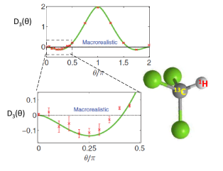
Figure 2: Information deficit $D_{3}$ versus $\theta$ obtained using INRM procedure. The mean experimental D3 values are shown as symbols. The curves indicate theoretical D3. The horizontal lines at D3 = 0 indicate the lower bounds of the macrorealism territories (Figure reproduced from reference Athalye et al. (2011a)).

As described in earlier, two sets of experiments were performed, one with CNOT and the other with anti-CNOT Athalye et al. (2011a). The joint entropies were calculated using the experimental probabilities and the information deficit (in bits) was calculated using the expression $D_{3}=2H(Q_{2}|Q_{1})-H(Q_{3}|Q_{1})$. The theoretical and experimental values of $D_{3}$ for various rotation angles $\theta$ are shown in Fig. 2. According to quantum theory, a maximum violation of $D_{3}=-0.134$ should occur at $\theta=\pi/4$. The corresponding experimental value, $D_{3}(\pi/4)=-0.114\pm 0.027$, indicates a clear violation of ELGI.

Our other experiments involving noninvasive measurements include (i) illustrating the inconsistency of quantum marginal probabilities with classical probability theory Athalye et al. (2011a) and (ii) demonstrating that quantum joint probabilities can not be obtained from moment distribution Karthik et al. (2013).

III Extracting expectation values

Often experimental setups allow direct detection of only a limited set of observables and to extract their expectation values. For example, in NMR only transverse magnetization operators ($\langle{\sigma_{x}}\rangle$ and $\langle{\sigma_{y}}\rangle)$ are directly observable via real and imaginary components of induced emf. Fig. 3 describes the circuits for measuring expectation values of different types of operators using an ancilla qubit. Here the expectation values $\langle{\sigma_{x}}\rangle$ and $\langle{\sigma_{y}}\rangle)$ of ancilla qubit reveal the expectation values of different types of operators acting on system qubit. Applications of such circuits are illustrated with the help of following experiments: (A) estimation of Franck-Condon factors, and (B) investigation of quantum contextuality.

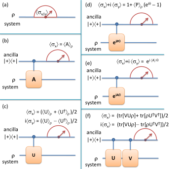
Figure 3: Circuits for (a) NMR measurements of $\langle{\sigma_{x}}\rangle$ and $\langle{\sigma_{y}}\rangle$, (b) standard Moussa protocol for expectation values of Hermitian-unitary operator $A$ Moussa et al. (2010), and circuits for measuring expectation values of (c) a unitary operator $U$ Joshi et al. (2014), (d) a projector $P$ Joshi et al. (2014) (e) a diagonal Hermitian operator $A$, and (f) for measuring joint expectation values of noncommuting unitaries $U$ and $V$Karthik et al. (2013).

III.1 Estimation of Franck-Condon factors

Franck-Condon principle states that the transition probability between two vibronic levels depends on the overlap between the respective vibrational wavefunctions Demtroder (2006). Franck-Condon factors (FCFs) dictate the intensities of vibronic transitions, and therefore their estimation is an important task in understanding absorption and fluorescence spectra and related phenomena such as photo-induced dissociations Bowers et al. (1984).

We modelled the electronic ground and excited vibrational levels as eigenstates of two harmonic potentials, $V_{1}$ and $V_{2}$ respectively. To simulate the one-dimensional case, we choose the potentials $V_{1}=x^{2}/2$ and $V_{2}=(x-b)^{2}/2+\Delta E$, which are identical up to an overall displacement $b$ in position and/or in energy $\Delta E$.

Thus the vibrational Hamiltonians for the two electronic states are

$${\cal H}_{1} = \textbf{p}^{2}/2+\textbf{x}^{2}/2$$

$${\cal H}_{2} = \textbf{p}^{2}/2+(\textbf{x}-b)^{2}/2+\Delta E.$$ (3)

The FCF between $|{m}\rangle$ of the electronic ground state and $|{n}\rangle$ of the electronic excited state is given by Demtroder (2006),

$$f_{m,n^{\prime}}(b) = |\langle m|n^{\prime}\rangle|^{2}$$ (5)

$$= \begin{array}[]{|c|}\int\limits_{-\infty}^{\infty}\psi_{m}^{*}(x)\psi_{n^{\prime}}(x,b)dx\end{array}^{2},$$

where $\psi_{m}(x)$, $\psi_{n^{\prime}}(x,b)$ are the corresponding position wave-functions.

Estimation of FCF, $f_{m,n^{\prime}}$, is equivalent to measurement of expectation value of the projection $P_{m}=|m\rangle\langle m|$ after preparing the system in excited state $|n^{\prime}\rangle$ since Joshi et al. (2014),

$$f_{m,n^{\prime}} = \langle n^{\prime}|m\rangle\langle m|n^{\prime}\rangle$$ (6)

$$= \langle P_{m}\rangle_{n^{\prime}}.$$

Three spin-1/2 ¹⁹F nuclei of iodotrifluoroethylene (C₂F₃I) dissolved in acetone-D₆ form a three-qubit NMR quantum simulator (see Fig. 4). $F_{1}$ qubit is chosen to be the ancilla and the other two qubits chosen representing the lowest four levels of the Harmonic oscillator Joshi et al. (2014). The vibrational levels of the electronic ground state are encoded onto the spin states such that $|{0}\rangle=|{\uparrow\uparrow}\rangle$, $|{1}\rangle=|{\uparrow\downarrow}\rangle$, $|{2}\rangle=|{\downarrow\uparrow}\rangle$, and $|{3}\rangle=|{\downarrow\downarrow}\rangle$. The preparation of excited state $|n^{\prime}\rangle$ can be achieved by first initializing the system in the corresponding state $|n\rangle$ of the electronic ground state and translating it in position from origin ($x=0$) to the point $x=b$. This translation was be achieved by the unitary operator

$$U_{T}(b)=e^{-i\textbf{p}b}.$$ (7)

Finally the expectation values $\langle{P_{m}}\rangle$ were measured experimentally using the circuit shown in Fig. 3d, and then the FCFs $f_{m,n}$ were obtained using eqn. 6 Joshi et al. (2014). The results described in Fig. 4 display a good correspondence with the theoretically expected values indicating the success of the experimental protocols.

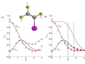
Figure 4: Experimental FCFs (circles) corresponding to 4-level harmonic oscillators versus the displacement $b$ (in atomic units). The simulated FCFs (dotted lines) for the 4-level system and analytical FCFs (smooth lines) for infinite-level system are also shown for comparison. The dashed curve at the top of (b) corresponds to the normalization used. The thin vertical dashed lines at $b=2,~{}1+\sqrt{3}$ mark the beginning of classically forbidden regions for $f_{0,0^{\prime}},f_{0,1^{\prime}}$ respectively. Molecular structure and qubit labelling are shown in the inset (Figure reproduced from reference Joshi et al. (2014)).

III.2 Investigation of quantum contextuality in a harmonic oscillator

Quantum contextuality (QC) states that the outcome of the measurement depends not only on the system and the observable but also on the context of the measurement, i.e., on other compatible observables which are measured along with Peres (1990). Consider the following NCHV inequality Nielsen and Chuang (2010a):

I $$=\langle{AB+BC+CD-AD}\rangle$$ (8)

$$=\langle{AB}\rangle+\langle{BC}\rangle+\langle{CD}\rangle-\langle{AD}\rangle\leq 2$$

Hong-Yi Su et.al. Su et al. (2012) theoretically studied QC of eigenstates of $1$D-QHO. They introduced two sets of pseudo-spin operators,

$$\Gamma_{x}=\sigma_{x}\otimes\mathbbm{1},~{}\Gamma_{y}=\sigma_{z}\otimes\sigma_{y},~{}\Gamma_{z}=-\sigma_{y}\otimes\sigma_{y},$$

$$\Gamma_{x}^{\prime}=\sigma_{x}\otimes\sigma_{z},~{}\Gamma_{y}^{\prime}=\mathbbm{1}\otimes\sigma_{y},~{}\Gamma_{z}^{\prime}=-\sigma_{x}\otimes\sigma_{x}.$$ (9)

where, $\mathbbm{1}$ is $2\times 2$ Identity matrix. Using these operators they defined the observables,

$$A=\Gamma_{x},B=c_{\beta}\Gamma_{x}^{\prime}+s_{\beta}\Gamma_{z}^{\prime}=\sigma_{x}\otimes(c_{\beta}\sigma_{z}-s_{\beta}\sigma_{x})$$

$$C=\Gamma_{z},~{}~{}D=c_{\eta}\Gamma_{x}^{\prime}+s_{\eta}\Gamma_{z}^{\prime}=\sigma_{x}\otimes(c_{\eta}\sigma_{z}-s_{\eta}\sigma_{x}),$$ (10)

where $c_{\beta}=\cos\beta,~{}s_{\beta}=\sin\beta,~{}c_{\eta}=\cos\eta$, and $s_{\eta}=\sin\eta$. Here operators $A,~{}B,~{}C,~{}D$ are unitary & Hermitian and accordingly have eigenvalues $\pm 1$, with $(A,B)$, $(B,C)$, $(C,D)$ and $(D,A)$ forming compatible pairs. Hong-Yi Su et.al. have shown that,

$$\mathrm{\textbf{I}}_{|{l}\rangle_{QHO}}^{QM}=2\sqrt{2}>2,~{}\mathrm{when},~{}(\beta,\eta)_{l}=\begin{cases}(-\pi/4,-3\pi/4)_{0}\\ (3\pi/4,\pi/4)_{1}\\ (\pi/4,3\pi/4)_{2}\\ (-3\pi/4,-\pi/4)_{3}\end{cases}$$ (11)

where, $\mathrm{\textbf{I}}_{|{l}\rangle_{QHO}}^{QM}$ is the expression on LHS of inequality 8, $l=0,1,2\textrm{ and }3$, and, $|{0}\rangle_{QHO},|{1}\rangle_{QHO},|{2}\rangle_{QHO}$ and $|{3}\rangle_{QHO}$ are first four energy eigenstates of 1D-QHO.

We encoded the first four energy eigenstates of 1D-QHO onto the four Zeeman eigenstates of a pair of spin-1/2 nuclei. The circuit shown in Fig. 3f was used to extract the expectation value of observables ($AB,BC,CD,$ and $DA$) in a joint measurement. We used three ¹⁹F nuclear spins of trifluoroiodoethylene dissolved in acetone-D6 (see inset of Fig. 4) as the 3-qubit register. The first spin, F₁, was used as an ancilla qubit, and other spins, F₂ and F₃, as the system qubits. The results are shown in Fig. 5. The maximum theoretical violation is $2\sqrt{2}=2.82$ Katiyar et al. (2015). The experimental value of maximum violation for $\mathrm{\textbf{I}}_{0},\mathrm{\textbf{I}}_{1},\mathrm{\textbf{I}}_{2},$ and $\mathrm{\textbf{I}}_{3}$ are $2.40\pm 0.017,~{}2.45\pm 0.025,~{}2.39\pm 0.016$, and $2.42\pm 0.026$ respectively Katiyar et al. (2015). There is a clear violation of the classical bound. Reduced violation than the theoretical value is due to $\mathrm{T}_{2}$ decay and inhomogeneity in Radio Frequency (RF) pulses.

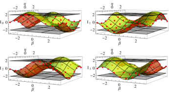
Figure 5: $\mathrm{\textbf{I}}_{0}$, $\mathrm{\textbf{I}}_{1}$, $\mathrm{\textbf{I}}_{2}$, and $\mathrm{\textbf{I}}_{3}$ represent evaluation of inequality 8 for eigenstates $|{0}\rangle_{QHO},|{1}\rangle_{QHO},|{2}\rangle_{QHO}$, and $|{3}\rangle_{QHO}$ respectively Katiyar et al. (2015). The curved surface represents theoretical values, and the points are experimental values. Flat planes at $I=2$ and $I=-2$ represent classical bounds.

IV Ancilla Assisted Quantum State Tomography

In experimental quantum information studies, Quantum State Tomography (QST) is an important tool that is routinely used to characterize an instantaneous quantum state Nielsen and Chuang (2010b). QST can be performed by a series of measurements of noncommuting observables which together enables one to reconstruct the complete complex density matrix Nielsen and Chuang (2010b). In the standard method, the required number of independent experiments grows exponentially with the number of input qubits I. L. Chuang and Leung (1998); Leung et al. (1999). Anil Kumar and co-workers have illustrated QST using a single two-dimensional NMR spectrum Das et al. (2003). Later Nieuwenhuizen and co-workers showed how to reduce the number of independent experiments in the presence of an ancilla register Allahverdyan et al. (2004). We referred to this method as Ancilla Assisted QST (AAQST) and experimentally demonstrated it using NMR systems Peng et al. (2007); Shukla et al. (2013). AAQST also allows single shot mapping of density matrix which not only reduces the experimental time, but also alleviates the need to prepare the target state repeatedly Shukla et al. (2013).

To see how AAQST works, consider an input register of $n$-qubits associated with an ancilla register consisting of $\hat{n}$ qubits. The dimension of the combined system of $\tilde{n}=n+\hat{n}$ qubits is $\tilde{N}=N\hat{N}$, where $\hat{N}=2^{\hat{n}}$. A completely resolved NMR spectrum yields $\tilde{n}\tilde{N}$ real parameters. We assume that the ancilla register begins with the maximally mixed initial state, with no contribution to the spectral lines from it. The deviation density matrix of the combined system is $\tilde{\rho}=\rho\otimes\mathbbm{1}/\hat{N}$. To perform AAQST, we apply a non-local unitary of the form,

$$\tilde{U}_{k}=V\sum\limits_{a=0}^{\hat{N}-1}U_{ka}\otimes|a\rangle\langle a|.$$ (12)

Here $U_{ka}$ is the $k$th unitary on the input register dependent on the ancilla state $|a\rangle$ and $V$ is the local unitary on the ancilla. The combined state evolves to

$$\tilde{\rho}^{(k)}=\tilde{U}_{k}\tilde{\rho}\tilde{U}_{k}^{\dagger}$$

$$=\frac{1}{\hat{N}}\sum\limits_{m,m^{\prime},a}\rho_{mm^{\prime}}U_{ka}|m\rangle\langle m^{\prime}|U_{ka}^{\dagger}\otimes V|a\rangle\langle a|V^{\dagger}.$$ (13)

Intensity of NMR spectrum is proportional to the observable $\sum\limits_{j=1}^{\tilde{n}}\sigma_{jx}+i\sigma_{jy}$. The spectrum of the combined system yields $\tilde{n}\tilde{N}$ linear equations. The minimum number of independent experiments needed is now $O(N^{2}/(\tilde{n}\tilde{N}))$. Choosing $\tilde{N}\gg N$, AAQST needs fewer than O($N/n$) experiments required in the standard QST. In particular, when $\tilde{n}\tilde{N}\geq N^{2}$, a single optimized unitary suffices for QST. Fig. 6 illustrates the minimum number ($K$) of experiments required for various sizes of input and ancilla registers. As illustrated, QST can be achieved with only one experiment, if an ancilla of sufficient size is provided along with Shukla et al. (2013).

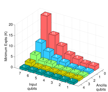
Figure 6: Minimum number of independent experiments required for QST (with zero ancilla) and AAQST (Figure reproduced from reference Shukla et al. (2013)).

To demonstrate this procedure experimentally, we used three ¹⁹F nuclei and two ¹H nuclei of 1-bromo-2,4,5-trifluorobenzene (BTFBz) partially oriented in a liquid crystal namely, N-(4-methoxybenzaldehyde)-4- butylaniline (MBBA) (Fig. 7) Shukla et al. (2013). We chose the three ¹⁹F nuclei forming the input register and two ¹H nuclei forming the ancilla register.

Fig 7 shows the experimental results corresponding to a particular density matrix obtained by applying unitary $U_{0}=\left(\frac{\pi}{2}\right)_{x}^{F}\tau_{0}(\pi)_{x}^{H}\tau_{0}\left(\frac{\pi}{2}\right)_{y}^{F_{1}},$ with $\tau_{0}=2.5$ ms, on thermal equilibrium state. The real and imaginary parts of the reconstructed density matrix along with the theoretically expected matrices are shown below the spectra in Fig. 7. Fidelity of the experimental state with the theoretical state was 0.95. The entire three-qubit density matrix with 63 unknowns was estimated by a single NMR experiment Shukla et al. (2013).

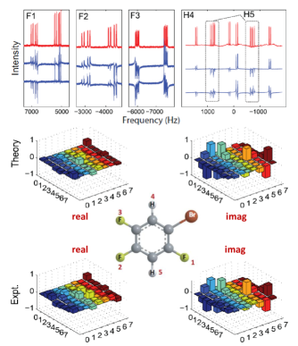
Figure 7: AAQST results for the state described in the text Shukla et al. (2013). The reference spectrum is in the top trace. The real (middle trace) and the imaginary spectra (bottom trace) are obtained in a single shot AAQST experiment. The bar plots correspond to theoretically expected density matrices (top row) and those obtained from AAQST experiments (bottom row). The molecular structure and the labelling scheme of BTFBz is shown in the center (Figure reproduced from reference Shukla et al. (2013)).

V Single Scan Process Tomography

Often one needs to characterize the overall process acting on a quantum system. Such a characterization, achieved by a procedure called quantum process tomography (QPT), is crucial in designing fault-tolerant quantum processors Chuang and Nielsen (1997); Poyatos et al. (1997). QPT is realized by considering the quantum process as a map from a complete set of initial states to final states, and experimentally characterizing each of the final states using QST I. L. Chuang and Leung (1998). Since QST by itself involves repeated preparations of a target state, QPT in general requires a number of independent experiments. Therefore the total number of independent measurements required for QPT increases exponentially with the size of the system undergoing the process.

The physical realization of QPT has been demonstrated on various experimental setups Childs et al. (2001); Weinstein et al. (2004); De Martini et al. (2003); Altepeter et al. (2003); O’Brien et al. (2004); Mitchell et al. (2003); Riebe et al. (2006); Hanneke et al. (2010); Neeley et al. (2008); Chow et al. (2009); Bialczak et al. (2010); Yamamoto et al. (2010); Chow et al. (2011); Dewes et al. (2012); Zhang et al. (2014). Several developments in the methodology of QPT have also been reported Shabani et al. (2011); Wu et al. (2013). In particular, it has been shown that ancilla assisted process tomography (AAPT) can characterize a process with a single QST Mazzei et al. (2003); De Martini et al. (2003); D’Ariano and Lo Presti (2003); Altepeter et al. (2003). By combining AAQST and AAPT, we showed that entire QPT can be carried out with a single ensemble measurement Shukla and Mahesh (2014). We referred to this procedure as ‘single-scan quantum process tomography’ (SSPT) Shukla and Mahesh (2014).

In the normal QPT procedure, the outcome of the process $\varepsilon$ is expanded in a complete basis of linearly independent elements $\{\rho_{1},\rho_{2},\cdots,\rho_{N^{2}}\}$ as well as using operator-sum representation, i.e.,

$$\varepsilon(\rho_{j})=\sum_{k}\lambda_{jk}\rho_{k}=\sum_{i}E_{i}\rho E_{i}^{\dagger}.$$ (14)

The complex coefficients $\lambda_{jk}$ can be extracted using QST. We can utilize a fixed set of basis operators $\{\tilde{E}_{m}\}$, and express $E_{i}=\sum_{m}e_{im}\tilde{E}_{m}$ so that

$$\varepsilon(\rho)=\sum_{mn}\tilde{E}_{m}\rho\tilde{E}_{n}^{\dagger}\chi_{mn},$$ (15)

where $\chi_{mn}=\sum_{i}e_{im}e_{in}^{*}$. The $\chi$ matrix completely characterizes the process $\varepsilon$. Since the set $\{\rho_{k}\}$ forms a complete basis, it is also possible to express

$$\tilde{E}_{m}\rho_{j}\tilde{E}_{n}^{\dagger}=\sum_{k}\beta_{jk}^{mn}\rho_{k},$$ (16)

where $\beta_{jk}^{mn}$ can be calculated theoretically. Using eqns. 14-16 and using the linear independence of $\{\rho_{k}\}$, we obtain

$$\beta\chi=\lambda,$$ (17)

from which $\chi$-matrix can be extracted by standard methods in linear algebra.

A comparison of QPT, AAPT, and SSPT procedures for a single qubit process is presented in Fig. 8 Shukla and Mahesh (2014).

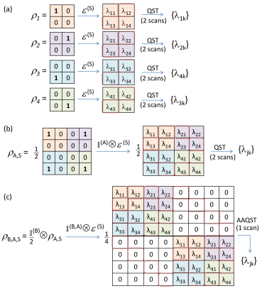
Figure 8: Illustrating (a) single-qubit QPT requiring a total of 8 NMR scans, (b) AAPT requiring 2 NMR scans, and (c) SSPT requiring a single-scan NMR experiment Shukla and Mahesh (2014). In each case, dotted lines are used to indicate the single-quantum elements of the density matrix which are directly observable. Other elements are observed by converting them to observable single-quantum coherences by using certain unitary operations in a subsequent scan(s) (Figure reproduced from reference Shukla and Mahesh (2014)).

Estimates of number of measurements for a small number of qubits shown in the first column of Table 1 illustrate the exponential increase of $M_{\mathrm{QPT}}$ with $n$.

$\begin{array}[]{|c|c|cc|cc|}\hline\cr n&M_{\mathrm{QPT}}&M_{\mathrm{AAPT}}&(n_{A})&M_{\mathrm{SSPT}}&(n_{A},n_{B})\\ \hline\cr\hline\cr 1&8&2&(1)&1&(1,1)\\ \hline\cr 2&32&4&(2)&1&(2,2)\\ \hline\cr 3&192&11&(3)&1&(3,3)\\ \hline\cr 4&1024&32&(4)&1&(4,5)\\ \hline\cr 5&7168&103&(5)&1&(5,6)\\ \hline\cr\end{array}$

Table 1: Comparison of number of scans and number of ancilla qubits (in parenthesis) required for $n$-qubit QPT, AAPT, and SSPT.

The experimental demonstration of a single-qubit SSPT was carried out using iodotrifluoroethylene dissolved in acetone-D₆ as a 3-qubit system Fig. 9 Shukla and Mahesh (2014). The experimentally obtained $\chi$ matrices for certain quantum processes using the single scan procedure are shown in Fig. 9.

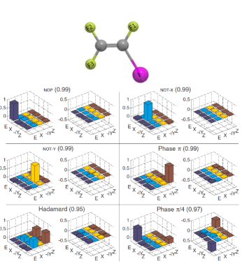
Figure 9: The barplots showing experimental $\chi$-matrices for various quantum processes obtained using SSPT. In each case, the left and right barplots correspond to the real and imaginary parts respectively, and the fidelities are indicated in parenthesis (Figure reproduced from reference Shukla and Mahesh (2014)).

VI Ancilla assisted noise engineering

Preserving coherence is a very important aspect to realize quantum processors, and hence various techniques have been developed to suppress decoherence. They include dynamical decoupling (DD) techniques Meiboom and Gill (1958); Viola et al. (1999); Viola and Lloyd (1998); Uhrig (2007), quantum error correction Preskill (1998), adiabatic quantum computation Farhi et al. (2000), and use of decoherence-free subspaces Lidar and Whaley (2003). Earlier Teklemariam et al. introduced artificial decoherence by achieving irreversible phase damping via constant perturbation of the environment qubits (by random classical fields), and thus mimicking a large dimensional environmental bath. Such experiments provide insights about decoherence processes and may pave the way for improving decoherence suppression techniques.

In our work we simulated such a decoherence process on a NMR simulator with two qubits, where one acts as the system and the other as environment Hegde and Mahesh (2014). We then subjected the system qubit to certain DD sequences and observed their competition with the engineered decoherence through noise spectroscopy.

The two qubit register was initially in the product state, $\rho(0)=\rho^{s}(0)\otimes\rho^{e}(0)$. Here $\rho^{s}(0)$ is the system state and $\rho^{e}(0)$ is the environment state. We chose ¹H and ¹³C nuclear spins in ¹³C-labelled chloroform (¹³CHCl₃ dissolved in CDCl₃) as the system and environment qubit respectively. The NMR Hamiltonian is

$${\cal H}=\pi(\nu_{s}\sigma_{z}^{s}+\nu_{e}\sigma_{z}^{e}+\frac{J}{2}\sigma_{z}^{s}\sigma_{z}^{e}),$$ (18)

where $\nu_{s}$ and $\nu_{e}$ are the resonant frequencies of the system and the environment qubits respectively, $J$ is the coupling strength between the two, and $\sigma_{z}^{s}$, $\sigma_{z}^{e}$ are the Pauli operators. In a total duration $T$, the propagator $U=e^{-i{\cal H}T}$ entangles the system qubit with the environment qubit via the interaction $J$. We engineered decoherence by a series of RF kicks of arbitrary angles $\epsilon\in[-\theta,\theta]$ on the environment qubit. These kicks induced artificial decoherence on the system qubit. Teklemariam et al. proved that induced decoherence of the system qubit depends on the kick-rate $\Gamma$, range of kick-angles $\theta$, and coupling strength $J$ Cory et al. (1998). Their model predicted that for small kick-angles $\epsilon$ and for lower kick rates $\Gamma$, decoherence rate $1/T_{2}$ increases linearly with $\Gamma$. After a certain value of $\Gamma$, $1/T_{2}$ saturates, and then onwards, it decreases exponentially with $\Gamma$.

Our experimental results for $\epsilon\in[0^{\circ},1^{\circ}]$ and $\Gamma=25$ kicks/ms are shown in Fig. 10 (indicated by stars). For comparison we have also shown the decay of magnetization without kicks (indicated by filled circles). Evidently, the kicks on environment have introduced additional decoherence thereby increasing the decay of system coherence Hegde and Mahesh (2014).

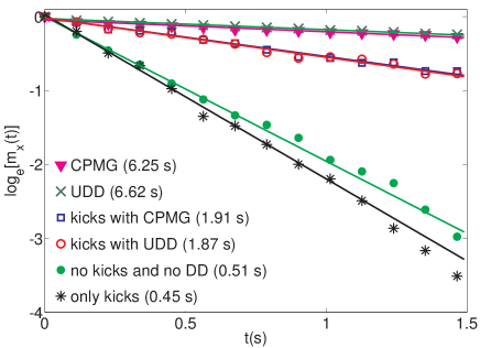
Figure 10: Logarithm of transverse magnetization $\log(M_{x})$ as a function of time under different pulse sequences as indicated in the legend. Here $\tau=3.2$ ms, $\Gamma=25$ kicks/ms, and $\epsilon\in[0^{\circ},1^{\circ}]$. The $T_{2}$ values for various pulse sequences are shown in the legend (Figure reproduced from reference Hegde and Mahesh (2014)).

Dynamical decoupling attempts to inhibit decoherence of system by rapid modulation of the system state so as to cancel the system-environment joint evolutions. The two standard DD sequences are: (i) CPMG Meiboom and Gill (1958) and (ii) UDD Uhrig (2007). CPMG consists of a series of equidistant $\pi$ pulses applied in the system qubits. In an N-pulse UDD of cycle time $t_{c}$, the time instant $t_{j}$ of $j^{\mathrm{th}}$ $\pi$-pulse is given by $t_{j}=t_{c}\sin^{2}\left[\frac{\pi j}{2(N+1)}\right]$. The results of the experiments for $t_{c}=22.4$ ms and with different kick-parameters are shown in Fig. 10. The competition between kicks-induced decoherence and DD sequences can be readily observed Hegde and Mahesh (2014).

Noise spectroscopy provides information about noise spectral density, which is the frequency distribution of noise and is helpful in not only understanding the performance of standard DD sequences, but also in optimizing them Biercuk et al. (2011, 2009); Pan et al. (2011). In the limit of a large number of $\pi$ pulses, the CPMG filter function resembles a delta peak at $\omega$, and samples this particular spectral frequency. The amplitude of the noise $S(\omega)$ can be determined by using the relation Yuge et al. (2011) $S(\omega)\simeq\frac{\pi^{2}}{4T_{2}(\omega)}$. Thus by measuring $T_{2}(\omega)$ for a range of $\omega=\pi/\tau$ values, we can scan the profile of $S(\omega)$.

The experimental spectral density profiles of only natural decoherence (lowest curve in each sub-plot), and with kicks of different kick-parameters are shown in Fig. 11 Hegde and Mahesh (2014). Clearly the effect of kicks is to increase the area under the spectral density profiles and thereby leading to faster decoherence. Moreover, for a given kick-rate $\Gamma$, larger the range of kick-angles, higher is the spectral density profile Hegde and Mahesh (2014).

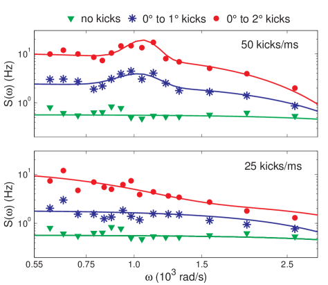
Figure 11: Experimental spectral density profiles with different kick-angles (as indicated in the legend) and with kick-rates 50 kicks/ms (top trace) and 25 kicks/ms (bottom trace). In both the traces, experimental spectral density profile without kicks is also shown for comparison. The smooth lines correspond to fits with one or two Gaussians (Figure reproduced from reference Hegde and Mahesh (2014)).

VII Summary

In this review article, we described several recent protocols for efficient measurements on quantum systems, and illustrated their NMR implementations.

In section II, we described ancilla-assisted noninvasive measurements, where the measurement result of an intermediate observable was temporarily stored in an ancilla qubit. A final joint-measurement of the system-ancilla register revealed the joint probabilities in a noninvasive way. We also showed the application of this technique in studying entropic Leggett-Garg inequality Athalye et al. (2011a).

In section III, we described extracting expectation values of various types of operators. Applications of these methods are illustrated in the estimation of Franck-Condon coefficients and in the investigation of quantum contextuality Joshi et al. (2014); Katiyar et al. (2015).

In section IV and V we described efficient ways to characterize quantum states and quantum process by exploiting ancilla qubits. We also illustrated single-scan quantum state tomography as well as single-scan quantum process tomography using NMR systems. These techniques not only alleviate the need of repeated measurements, but also allow the study of random states or dynamic processes Shukla et al. (2013); Shukla and Mahesh (2014).

Finally in section VI we described ancilla-assisted noise engineering, where random fields applied to the ancilla qubits cause controllable decoherence on the system qubits. We illustrated this phenomena using a two-qubit NMR system, and studied the engineered decoherence by measuring noise spectrum Hegde and Mahesh (2014).

Although we have used NMR techniques to demonstrate the above protocols experimentally, these procedures are quite general in nature, and can easily be adopted to other experimental techniques as well.

VIII Acknowledgements

The authors are grateful to Prof. Anil Kumar of IISc Bangalore, Prof. Usha Devi of Bangalore University, Prof. A. K. Rajagopal of Inspire Institute, USA, and Dr. Anirban Hazra of IISER, Pune for discussions. Projects described in this article were partly supported by DST Project No. SR/S2/LOP-0017/2009.

References

- Athalye et al. (2011a) V. Athalye, S. S. Roy, and T. S. Mahesh, Phys. Rev. Lett. 107, 130402 (2011a).
- Knee et al. (2012a) G. C. Knee, E. M. Gauger, G. A. D. Briggs, and S. C. Benjamin, New Journal of Physics 14, 058001 (2012a).
- Leggett and Garg (1985) A. J. Leggett and A. Garg, Phys. Rev. Lett. 54, 857 (1985).
- Palacios-Laloy et al. (2010) A. Palacios-Laloy, F. Mallet, F. Nguyen, P. Bertet, D. Vion, D. Esteve, and A. N. Korotkov, Nature Physics 6, 442 (2010).
- Athalye et al. (2011b) V. Athalye, S. S. Roy, and T. S. Mahesh, Physical review letters 107, 130402 (2011b).
- Lambert et al. (2011) N. Lambert, R. Johansson, and F. Nori, Phys. Rev. B 84, 245421 (2011).
- Goggin et al. (2011) M. Goggin, M. Almeida, M. Barbieri, B. Lanyon, J. O’Brien, A. White, and G. Pryde, Proceedings of the National Academy of Sciences 108, 1256 (2011).
- Dressel et al. (2011) J. Dressel, C. J. Broadbent, J. C. Howell, and A. N. Jordan, Phys. Rev. Lett. 106, 040402 (2011).
- Souza et al. (2011) A. Souza, I. Oliveira, and R. Sarthour, New Journal of Physics 13, 053023 (2011).
- Emary (2012) C. Emary, Phys. Rev. B 86, 085418 (2012).
- Suzuki et al. (2012) Y. Suzuki, M. Iinuma, and H. F. Hofmann, New Journal of Physics 14, 103022 (2012).
- Yong-Nan et al. (2012) S. Yong-Nan, Z. Yang, G. Rong-Chun, T. Jian-Shun, and L. Chuan-Feng, Chinese Physics Letters 29, 120302 (2012).
- Zhou et al. (2012) Z.-Q. Zhou, S. F. Huelga, C.-F. Li, and G.-C. Guo, arXiv preprint arXiv:1209.2176 (2012).
- Knee et al. (2012b) G. C. Knee, S. Simmons, E. M. Gauger, J. J. Morton, H. Riemann, N. V. Abrosimov, P. Becker, H.-J. Pohl, K. M. Itoh, M. L. Thewalt, et al., Nature communications 3, 606 (2012b).
- Devi et al. (2013) A. R. U. Devi, H. S. Karthik, Sudha, and A. K. Rajagopal, Phys. Rev. A 87, 052103 (2013).
- Karthik et al. (2013) H. S. Karthik, H. Katiyar, A. Shukla, T. S. Mahesh, A. R. U. Devi, and A. K. Rajagopal, Phys. Rev. A 87, 052118 (2013).
- Moussa et al. (2010) O. Moussa, C. A. Ryan, D. G. Cory, and R. Laflamme, Phys. Rev. Lett. 104, 160501 (2010).
- Joshi et al. (2014) S. Joshi, A. Shukla, H. Katiyar, A. Hazra, and T. S. Mahesh, Physical Review A 90, 022303 (2014).
- Demtroder (2006) W. Demtroder, Heidelberg, Springer-Verlag Berlin Heidelberg, 2006. 571 (2006).
- Bowers et al. (1984) W. D. Bowers, S. S. Delbert, R. L. Hunter, and R. T. McIver Jr, Journal of the American Chemical Society 106, 7288 (1984).
- Peres (1990) A. Peres, Physics Letters A 151, 107 (1990).
- Nielsen and Chuang (2010a) M. A. Nielsen and I. L. Chuang, Quantum Computation and Quantum Information (Cambridge University Press, 2010) cambridge Books Online.
- Su et al. (2012) H.-Y. Su, J.-L. Chen, C. Wu, S. Yu, and C. H. Oh, Phys. Rev. A 85, 052126 (2012).
- Katiyar et al. (2015) H. Katiyar, C. Kumar, and T. S. Mahesh, arXiv preprint arXiv:1503.05883 (2015).
- Nielsen and Chuang (2010b) Nielsen and I. L. Chuang, Quantum computation and quantum information (Cambridge university press, 2010).
- I. L. Chuang and Leung (1998) M. G. K. I. L. Chuang, N. Gershenfeld and D. W. Leung, Proc. R. Soc. Lond.,Ser A 454, 447 (1998).
- Leung et al. (1999) D. Leung, L. Vandersypen, X. Zhou, M. Sherwood, C. Yannoni, M. Kubinec, and I. Chuang, Physical Review A 60, 1924 (1999).
- Das et al. (2003) R. Das, T. S. Mahesh, and A. Kumar, Phys. Rev. A 67, 062304 (2003).
- Allahverdyan et al. (2004) A. E. Allahverdyan, R. Balian, and T. M. Nieuwenhuizen, Phys. Rev. Lett. 92, 120402 (2004).
- Peng et al. (2007) X. Peng, J. Du, and D. Suter, Phys. Rev. A 76, 042117 (2007).
- Shukla et al. (2013) A. Shukla, K. R. K. Rao, and T. S. Mahesh, Phys. Rev. A 87, 062317 (2013).
- Chuang and Nielsen (1997) I. L. Chuang and M. A. Nielsen, Journal of Modern Optics 44, 2455 (1997).
- Poyatos et al. (1997) J. F. Poyatos, J. I. Cirac, and P. Zoller, Phys. Rev. Lett. 78, 390 (1997).
- Childs et al. (2001) A. M. Childs, I. L. Chuang, and D. W. Leung, Phys. Rev. A 64, 012314 (2001).
- Weinstein et al. (2004) Y. S. Weinstein, T. F. Havel, J. Emerson, N. Boulant, M. Saraceno, S. Lloyd, and D. G. Cory, The Journal of Chemical Physics 121, 6117 (2004).
- De Martini et al. (2003) F. De Martini, A. Mazzei, M. Ricci, and G. M. D’Ariano, Phys. Rev. A 67, 062307 (2003).
- Altepeter et al. (2003) J. B. Altepeter, D. Branning, E. Jeffrey, T. C. Wei, P. G. Kwiat, R. T. Thew, J. L. O’Brien, M. A. Nielsen, and A. G. White, Phys. Rev. Lett. 90, 193601 (2003).
- O’Brien et al. (2004) J. L. O’Brien, G. J. Pryde, A. Gilchrist, D. F. V. James, N. K. Langford, T. C. Ralph, and A. G. White, Phys. Rev. Lett. 93, 080502 (2004).
- Mitchell et al. (2003) M. W. Mitchell, C. W. Ellenor, S. Schneider, and A. M. Steinberg, Phys. Rev. Lett. 91, 120402 (2003).
- Riebe et al. (2006) M. Riebe, K. Kim, P. Schindler, T. Monz, P. O. Schmidt, T. K. Körber, W. Hänsel, H. Häffner, C. F. Roos, and R. Blatt, Phys. Rev. Lett. 97, 220407 (2006).
- Hanneke et al. (2010) D. Hanneke, J. P. Home, J. D. Jost, J. M. Amini, D. Leibfried, and D. J. Wineland, Nature Phys. 6, 13 (2010).
- Neeley et al. (2008) M. Neeley, M. Ansmann, R. C. Bialczak, M. Hofheinz, N. Katz, E. Lucero, A. O/’Connell, H. Wang, A. N. Cleland, and J. M. Martinis, Nature Phys. 4, 523 (2008).
- Chow et al. (2009) J. M. Chow, J. M. Gambetta, L. Tornberg, J. Koch, L. S. Bishop, A. A. Houck, B. R. Johnson, L. Frunzio, S. M. Girvin, and R. J. Schoelkopf, Phys. Rev. Lett. 102, 090502 (2009).
- Bialczak et al. (2010) R. C. Bialczak, M. Ansmann, M. Hofheinz, E. Lucero, M. Neeley, A. D. O/’Connell, D. Sank, H. Wang, J. Wenner, M. Steffen, and J. M. Cleland, A. N.and Martinis, Nature Phys. 6, 409 (2010).
- Yamamoto et al. (2010) T. Yamamoto, M. Neeley, E. Lucero, R. C. Bialczak, J. Kelly, M. Lenander, M. Mariantoni, A. D. O’Connell, D. Sank, H. Wang, M. Weides, J. Wenner, Y. Yin, A. N. Cleland, and J. M. Martinis, Phys. Rev. B 82, 184515 (2010).
- Chow et al. (2011) J. M. Chow, A. D. Córcoles, J. M. Gambetta, C. Rigetti, B. R. Johnson, J. A. Smolin, J. R. Rozen, G. A. Keefe, M. B. Rothwell, M. B. Ketchen, and M. Steffen, Phys. Rev. Lett. 107, 080502 (2011).
- Dewes et al. (2012) A. Dewes, F. R. Ong, V. Schmitt, R. Lauro, N. Boulant, P. Bertet, D. Vion, and D. Esteve, Phys. Rev. Lett. 108, 057002 (2012).
- Zhang et al. (2014) J. Zhang, A. M. Souza, F. D. Brandao, and D. Suter, Phys. Rev. Lett. 112, 050502 (2014).
- Shabani et al. (2011) A. Shabani, R. L. Kosut, M. Mohseni, H. Rabitz, M. A. Broome, M. P. Almeida, A. Fedrizzi, and A. G. White, Phys. Rev. Lett. 106, 100401 (2011).
- Wu et al. (2013) Z. Wu, S. Li, W. Zheng, X. Peng, and M. Feng, The Journal of Chemical Physics 138, 024318 (2013).
- Mazzei et al. (2003) A. Mazzei, M. Ricci, F. De Martini, and G. D’Ariano, Fortschritte der Physik 51, 342 (2003).
- D’Ariano and Lo Presti (2003) G. M. D’Ariano and P. Lo Presti, Phys. Rev. Lett. 91, 047902 (2003).
- Shukla and Mahesh (2014) A. Shukla and T. S. Mahesh, Physical Review A 90, 052301 (2014).
- Meiboom and Gill (1958) S. Meiboom and D. Gill, Rev. of Sci. Instrum. 29, 688 (1958).
- Viola et al. (1999) L. Viola, E. Knill, and S. Lloyd, Phys. Rev. Lett. 82, 2417 (1999).
- Viola and Lloyd (1998) L. Viola and S. Lloyd, Phys. Rev. A 58, 2733 (1998).
- Uhrig (2007) G. S. Uhrig, Phys. Rev. Lett. 98, 100504 (2007).
- Preskill (1998) J. Preskill, Proc. R. Soc. Lond. A 454, 385 (1998).
- Farhi et al. (2000) E. Farhi, J. Goldstone, S. Gutmann, and M. Sipser, arXiv:quant-ph/0001106 (2000).
- Lidar and Whaley (2003) D. A. Lidar and K. B. Whaley, in Irreversible Quantum Dynamics (Springer, 2003) pp. 83–120.
- Hegde and Mahesh (2014) S. S. Hegde and T. S. Mahesh, Physical Review A 89, 062317 (2014).
- Cory et al. (1998) D. G. Cory, M. D. Price, and T. F. Havel, Physica D 120, 82 (1998).
- Biercuk et al. (2011) M. Biercuk, A. Doherty, and H. Uys, J. Phys. B 44, 154002 (2011).
- Biercuk et al. (2009) M. J. Biercuk, H. Uys, A. P. VanDevender, N. Shiga, W. M. Itano, and J. J. Bollinger, Nature 458, 996 (2009).
- Pan et al. (2011) Y. Pan, Z.-R. Xi, and J. Gong, J. Phys. B 44, 175501 (2011).
- Yuge et al. (2011) T. Yuge, S. Sasaki, and Y. Hirayama, Phys. Rev. Lett. 107, 170504 (2011).