Multivariate Topology Simplification

Abstract

Topological simplification of scalar and vector fields is well-established as an effective method for analysing and visualising complex data sets. For multi-field data, topological analysis requires simultaneous advances both mathematically and computationally. We propose a robust multivariate topology simplification method based on “lip”-pruning from the Reeb Space. Mathematically, we show that the projection of the Jacobi Set of multivariate data into the Reeb Space produces a Jacobi Structure that separates the Reeb Space into simple components. We also show that the dual graph of these components gives rise to a Reeb Skeleton that has properties similar to the scalar contour tree and Reeb Graph, for topologically simple domains. We then introduce a range measure to give a scaling-invariant total ordering of the components or features that can be used for simplification. Computationally, we show how to compute Jacobi Structure, Reeb Skeleton, Range and Geometric Measures in the Joint Contour Net (an approximation of the Reeb Space) and that these can be used for visualisation similar to the contour tree or Reeb Graph.

keyword

Simplification, Topology, Multi-Field, Reeb Space, Joint Contour Net, Multi-Dimensional Reeb Graph, Reeb Skeleton

1 Introduction

Scientific data is often complex in nature and difficult to visualise. As a result, analytic tools have become increasingly prominent in scientific visualisation, and in particular topological analysis. While earlier work dealt primarily with scalar data [33, 6, 54], multivariate topological analysis in the form of the Reeb Space [48, 19] has started to become feasible using a quantised approximation called the Joint Contour Net (JCN) [7].

Prior experience in scalar and vector topology shows that simplification of topological structures is required, as real data sets are often noisy and complex. Although most of the work required is practical and algorithmic in nature, mathematical formalisms are also needed, in this case based on fiber analysis, in the same way that Reeb Graphs and contour trees rely on Morse theory. This paper therefore:

1. Clarifies relationships between the Reeb Space of a multivariate map $f$, the Jacobi Set of $f$, and fiber topology,

2. Introduces the Jacobi Structure in the Reeb Space that decomposes the Reeb Space into regular and singular components equivalent to edges and vertices in the Reeb Graph, then reduces it further to a Reeb Skeleton,

3. Proves that Reeb Spaces for topologically simple domains have simple structures with properties analogous to properties of the contour tree, allowing lip-pruning based simplification,

4. Introduces the range measure and other geometric measures for a total ordering of regular components of the Reeb Space,

5. Describes an algorithm that extracts the Jacobi Structure from the Joint Contour Net using a Multi-dimensional Reeb Graph (MDRG) and computes the Reeb Skeleton, and

6. Simplifies the Reeb Skeleton and the corresponding Reeb Space computing the range and other geometric measures using the Joint Contour Net.

To clarify the relationships between the newly introduced data-structures in the current paper, note that the JCN is an approximation of the Reeb Space. We compute a MDRG from the JCN. The critical nodes of the MDRG form the Jacobi Structure of the JCN. The Jacobi Structure then separates the JCN into regular and singular components. The dual graph of such components gives a Reeb Skeleton which is used in the multivariate topology simplification.

As a result, much of this paper addresses the theoretical machinery for simplification of the Reeb Space and its approximation, the Joint Contour Net.  Section 2 reviews relevant background material on simplification, followed by a more detailed review of the fiber topology, Jacobi Set and Reeb Space in Section 3. Section 4 provides theoretical analysis and results needed for the lip-simplification of the Reeb Space. For simple domains, the Reeb Space can have detachable (lip) components: this is used in Section 5 to generalise leaf-pruning simplification from the contour tree to the Reeb Space. Once this has been done, we introduce a range persistence and other geometric measures to govern the simplification process.

In Section 6, we give an algorithm for simplifying the Joint Contour Net (an approximation of the Reeb Space). We start by building a hierarchical structure called the Multi-Dimensional Reeb Graph (MDRG) that captures the Jacobi Structure of the Joint Contour Net, and then show how to reduce the JCN to a Reeb Skeleton - a graph with properties similar to a contour tree. In Section 7, we illustrate these reductions first with analytic data where the correct solution is known a priori, then for a real data from the nuclear physics. As part of this, we provide performance figures and other implementation details in Section 7, then draw conclusions and lay out a road map for further work in Section 8.

2 Previous Work

Topology-based simplification aims to reduce the topological complexity of the underlying data. There are different ways to measure such topological complexity depending on the nature of the underlying data. Here we mention some well-known approaches from the literature for measuring the topological complexity and their simplification procedure.

Scalar Field Simplification.

The topological complexity of the scalar field data is measured in terms of the number of critical points and their connectivities - captured by its Reeb Graph or contour tree. Another way to capture the topological complexity of the scalar field is by computing the Morse-Smale complex of the corresponding gradient field. Therefore, the topological simplification in this case is driven by reducing the number of critical points via simplification of the Reeb Graph/ contour tree or the Morse-Smale complex. Carr et al. [6] describe a method for associating local geometric measures such as the surface area and the contained volume of contours with the contour tree and then simplifying the contour tree by suppressing the minor topological features of the data. Note that a feature is any prominent or distinctive part or quality that characterises the data and topological features captures the topological phenomena of the underlying data. Wood et al. [58] give a Reeb Graph based simplification strategy for removing the excess topology created by unwanted handles in an isosurface using a measure for computing the handle-size in the isosurface and associating them with the loops of the Reeb Graph. Gyulassy et al. [24] describe a technique for simplifying a three-dimensional scalar field by repeatedly removing pair of critical points from the Morse-Smale complex of its gradient field, by repeated application of a critical-point simplification operation. Mathematically, the simplification of “lips” proposed in this paper is a direct generalization of this idea (for scalar fields) to multi-fields. Luo et al [37] describe a method for computing and simplifying gradients and critical points of a function from a point cloud. Tierny et al. [54] present a combinatorial algorithm for simplifying the topology of a scalar field on a surface by approximating with a simpler scalar field having a subset of critical points of the given field, while guaranteeing a small error distance between the fields.

The topological complexity of a point cloud data can be measured by its homology. For a point cloud data in $\mathbb{R}^{3}$ this is expressed by the topological invariants, such as the Betti numbers corresponding to a simplicial complex of the point cloud - denoted by $\beta_{0}$ (number of connected components), $\beta_{1}$ (number of tunnels or 1-dimensional holes) and $\beta_{2}$ (number of voids or 2-dimensional holes). The $i$-th Betti number represents the rank of the $i$-th homology group ($i=0,1,2$). Edelsbrunner et al. [20] introduce the idea of persistence homology for the topological simplification of a point cloud by reducing the Betti numbers using a filtration technique. Cohen-Steiner et al. [12] extend the persistence diagram for scalar functions on topological spaces and analyze its stability.

Mesh Simplification.

Mesh-simplification is well-known in the computational geometry and graphics community. Topological complexity of a mesh can be determined by its genus. Guskov et al. [23] remove the unnecessary topological noise from meshes of laser scanner data by reducing their genera. Nooruddin et al. [40] give a voxel-based simplification and repair method of polygonal models using a volumetric morphological operation. Ni et al. [39] generate a fair Morse function for extracting the topological structure of a surface mesh by user-controlled number and configuration of critical points. Hoppe et al. [30] describe a energy-minimization technique for generating an optimal mesh by reducing the number of vertices from a given mesh. Also Hoppe et al. [29, 44] give a new progressive mesh representation, a new scheme for storing and transmitting arbitrary triangle meshes, and their simplification technique. Chiang et al. [33] describe a technique of progressive simplification of tetrahedral meshes preserving isosurface topologies. Their method works in two stages - first they segment the volume data into topological-equivalence regions and in the second step they simplify each topological-equivalence region independently by edge collapsing, preserving the iso-surface topologies. There are many cost-driven methods of mesh-simplification (in the literature) which attempt to measure only the cost of each individual edge collapse and the entire simplification process is considered as a sequence of steps of increasing cost [13, 35, 36, 21].

Vector Field Simplification.

Topology based methods for vector field simplification are based on the idea of singularity pair cancellation to reduce the number of singularities and thus the topological complexity. This method iteratively eliminates suitable pairs of singularities with opposite Poincaré-Hopf indices so that total sum of the indices remain invariant to keep the global structure of the field the same. This idea has been exploited in [56, 59, 45]. There are also non-topology based methods for vector-field simplification which are mainly based on smoothing operations. Smoothing operations reduce vector and tensor-field complexity and remove large percentage of singularities. Polthier et al. [43] apply Laplacian smoothing on the potential of a vector-field. Tong et al. [55] decompose a vector field into three components: curl free, divergence free and harmonic. Each component is smoothed individually and results are summed to obtain simplified vector field.

Multi-Field Simplification.

To the best of our knowledge, until now there is no prior work on topology-based simplification of general multi-field data. All those techniques, cited so far, for simplifying scalar fields, meshes and vector fields are not directly applicable in case of multi-fields, mainly because the computation of the equivalent tools such as, Jacobi Set [18], Reeb Space [19] are not well-developed. A generalization of the persistence homology is proven to be difficult for the multi-fields [4]. However, few attempts have been made for simplifying the Jacobi Sets in restrictive cases. Snyder et al. [50] give two metrics for measuring persistence of the Jacobi Sets. Bremer et al. [3] describe a method for noise removal from the Jacobi Sets of time varying data. Suthambhara et al. [52] give a technique for the Jacobi Set simplification of bivariate fields based on simplification of the Reeb Graphs of their comparison measures. Huettenberger et al. propose multi-field simplification method using Pareto sets [31, 32]. However, these methods lack mathematical justification for simplifying the corresponding input multi-fields and work mostly for bivariate data. In a similar context, Bhatia et al. [2] provide a simplification method by generalising the critical point cancellation of scalar functions to the Jacobi Sets in two dimensional domains.

However, current research shows that the Jacobi Sets are unable to capture the actual topological changes of multi-fields, instead one should consider their Reeb Spaces, introduced in [19]. Recently, Multi-Dimensional Reeb Graphs [10] and Layered Reeb Graphs [51] have been introduced from two different perspectives to extend the Reeb Graph for multi-fields. In the current paper, we use the recently introduced Jacobi Structure [10] to separate the Reeb Space into regular and singular components. Thus we obtain a dual Reeb Skeleton corresponding to the Reeb Space. Our simplification strategy is based on simplifying this Reeb Skeleton by associating different measures with the nodes of the Reeb Skeleton.

3 Necessary Background

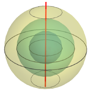
(a)

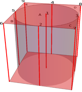
(b)

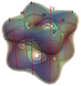
(c)

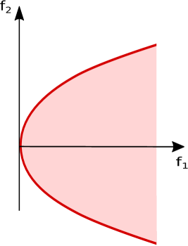
(d)

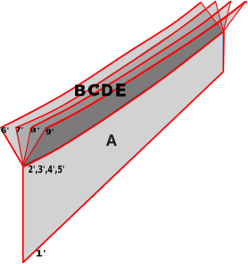
(e)

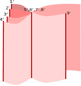
(f)

Figure 1: (a) A stable bivariate field $(f_{1},f_{2})\equiv(x^{2}+y^{2}+z^{2},\,z)$ from $\mathbb{R}^{3}$ to $\mathbb{R}^{2}$ that is visualized using the transparent isosurfaces of the first component field; black curves are the fiber-components of the bivariate field; the red line represents the Jacobi Set; (d) The Reeb Space corresponding to (a) that is comprising one sheet (in pink) and the Jacobi Structure (red parabolic curve); (b) The Jacobi Set (consists of the red lines, top face and bottom face of the box) of the bivariate field $(f_{1},f_{2})\equiv(x^{2}+y^{2}+z^{2},\,z)$ in the box $[-1,\,1]\times[-1,\,1]\times[0,\,1]$; singular fibers passing through the boundary tangent points form a cylindrical surface that separates the domain into five components, denoted as A, B, C, D and E; (e) The Reeb Space of the multi-field corresponding to (b) that is comprising five sheets (in grey) and the Jacobi Structure (red lines); the regular components of the Reeb Space are marked to match the corresponding components in the domain; components of the Jacobi Set in the domain and their corresponding projections in the Reeb Space are denoted by numbers; (c) An unstable bivariate field $(f_{1},f_{2})\equiv(x^{4}+y^{4}+z^{4}-5(x^{2}+y^{2}+z^{2})+10,\,z)$ from $\mathbb{R}^{3}$ to $\mathbb{R}^{2}$ that is visualized using the transparent isosurfaces of the first component field; black curves are the fiber-components of the bivariate field; the Jacobi Set consists of 9 red lines; (f) The Reeb Space corresponding to (c) that is comprising six sheets and the Jacobi Structure (6 red lines).

Over the last two decades, scalar topology has been used to support scientific data analysis and visualization, in particular through the use of the Reeb Graph and its specialisation, the contour tree [57, 8, 26, 17, 41]. The subject of multi-field topology in data analysis is rather new. In this section we briefly describe the multi-field topological analysis and existing tools for capturing them, viz. the Jacobi Set and the Reeb Space.

Table 1: Important Notations

Notation	Name
$\mathbb{W}_{f}$	Reeb Space
$\mathbb{K}_{f}$	Reeb Skeleton
$\mathbb{J}_{f}$	Jacobi Set
${\mathbb{J}}^{\partial}_{f}$	Boundary Jacobi Set
${\mathbb{J}}^{\circ}_{f}$	Interior Jacobi Set
$\mathfrak{J}_{f}$	Jacobi Structure
$JCN(\,f,m_{Q})$	Joint Contour Net with quantization level $m_{Q}$
$\mathbb{R}_{f_{i}}$	Reeb Graph
$\mathbb{M}_{f}$	Multi-dimensional Reeb Graph

Multi-Field Analysis.

A multi-field on a $d$-manifold $\mathbb{X}\,(\subseteq\mathbb{R}^{d})$ with $r$ component scalar fields $f_{i}:\mathbb{X}\rightarrow\mathbb{R}$ ($i=1,\,\ldots,r$) is a map $f=(f_{1},\,f_{2},\,\ldots,\,f_{r}):\mathbb{X}\rightarrow\mathbb{R}^{r}$. Table 1 shows the notations used to denote various structures corresponding to a multi-field $f$ in the current paper.

In differential topology, $f$ is considered to be a smooth map when all its partial derivatives of any order are continuous. A point $\mathbf{x}\in\mathbb{X}$ is called a singular point (or critical point) of $f$ if the rank of its differential map $df_{\mathbf{x}}$ is strictly less than $\min\{d,r\}$ where $df_{\mathbf{x}}$ is the $r\times d$ matrix whose rows are the gradients of $f_{1}$ to $f_{r}$ at $\mathbf{x}$. And the corresponding value $f(\mathbf{x})=\mathbf{c}=(c_{1},\,c_{2},\,\ldots,\,c_{r})$ in $\mathbb{R}^{r}$ is a singular value. Otherwise if the rank of the differential map $df_{\mathbf{x}}$ is $\min\{d,r\}$ then $\mathbf{x}$ is called a regular point and a point $\mathbf{y}\in\mathbb{R}^{r}$ is a regular value if $f^{-1}(\mathbf{y})$ does not contain a singular point.

The inverse image of the map $f$ corresponding to a value $\mathbf{c}\in\mathbb{R}^{r}$, $f^{-1}(\mathbf{c})$ is called a fiber and each connected component of the fiber is called a fiber-component [49, 48]. In particular, for a scalar field these are known as the level set and the contour, respectively. The inverse image of a singular value is called a singular fiber and the inverse image of a regular value is called a regular fiber. If a fiber-component passes through a singular point, it is called a singular fiber-component. Otherwise, it is known as a regular fiber-component. Note that a singular fiber may contain a regular fiber-component.

A continuous map is said to be proper if the pre-image of a compact set is always compact and it is said to be stable if its topological properties remain unchanged by small perturbations [28]. Let $f:\mathbb{X}\subset\mathbb{R}^{3}\to\mathbb{R}^{2}$ be a proper smooth map. Then, it is stable if and only if it satisfies the following local and global conditions. Around each singular point $\mathbf{s}$, $f$ is locally described as either (i) $(u,\,x^{2}+y^{2})$: $\mathbf{s}$ is a definite fold point, or (ii) $(u,\,x^{2}-y^{2})$: $\mathbf{s}$ is an indefinite fold point, or (iii) $(u,\,y^{2}+ux-x^{3}/3)$: $\mathbf{s}$ is a cusp point, for some local coordinates $(u,\,x,\,y)$ around $\mathbf{s}$ and an appropriate set of local coordinates around $f(\mathbf{s})$ in the range $\mathbb{R}^{2}$. Moreover, no cusp point is a double point of $f$ restricted to the set of singular points and $f$ restricted to the set of all definite and indefinite fold points is an immersion with normal crossings. Thus for a proper stable map, a singular fiber-component passing through a definite fold point or a cusp point contains exactly one such point, while a singular fiber-component passing through an indefinite fold point may pass through one or two indefinite fold points. Otherwise, the map is called an unstable map.

We note, characterizing the stability of the maps on compact 3-manifold domains with boundary needs additional types of singularities which is discussed in [47]. Figure 1a is an example of a map from $\mathbb{R}^{3}$ to $\mathbb{R}^{2}$ where $f=(x^{2}+y^{2}+z^{2},\,z)$. All its singular points are definite fold points, so this is an example of a stable map. Figure 1c is an example of a map from $\mathbb{R}^{3}$ to $\mathbb{R}^{2}$ where $f=(x^{4}+y^{4}+z^{4}-5(x^{2}+y^{2}+z^{2})+10,\,z)$. It has singular fiber-components which pass through four indefinite fold points (on corresponding four 1-manifold components numbered as 5, 6, 7 and 8 in Figure 1c) and so is an example of an unstable map.

From the pre-image theorem [22], generically a regular fiber $f^{-1}(\mathbf{c})$ is a $(d-r)$-manifold for the regular value $\mathbf{c}=(c_{1},\,c_{2},\,\ldots,\,c_{r})$. We note for $d<r$, $f^{-1}(\mathbf{c})$ is an empty set or a discrete set of points. A fiber $f^{-1}(\mathbf{c})$ can be considered as the intersection of the fibers of the component scalar fields $f_{1}^{-1}(c_{1}),\,f_{2}^{-1}(c_{2}),\ldots,\,f_{r}^{-1}(c_{r})$ and a connected component of this intersection is a fiber-component. Alternatively, fiber-components of $(f_{1},\,f_{2},\,\ldots,\,f_{r})$ can be considered as the contours of a component field $f_{i}$, restricted to the fiber-components of the remaining component fields. This is a key observation, we use in building our Multi-Dimensional Reeb Graph data-structure.

Jacobi Set.

The compact $d$-manifold domain $\mathbb{X}\,(\subseteq\mathbb{R}^{d})$ of the map $f$ can be expressed as $\mathbb{X}={\mathbb{X}}^{\circ}\cup\partial\mathbb{X}$ where ${\mathbb{X}}^{\circ}$ denotes the interior (the set of interior points) of the domain and $\partial\mathbb{X}$ denotes the boundary (the set of boundary points) of $\mathbb{X}$. In case the domain $\mathbb{X}$ is without boundary, $\partial\mathbb{X}=\emptyset$ and $\mathbb{X}={\mathbb{X}}^{\circ}$.

Now the interior Jacobi Set of the map $f:\mathbb{X}\rightarrow\mathbb{R}^{r}$ is denoted by ${\mathbb{J}}^{\circ}_{f}$ and is defined by the set ${\mathbb{J}}^{\circ}_{f}:=\left\{\mathbf{x}\in{\mathbb{X}}^{\circ}\mid\text{ rank }d{f}^{\circ}_{x}<\min\{d,r\}\right\}$ [16] where ${f}^{\circ}$ is the restriction of $f$ to ${\mathbb{X}}^{\circ}$, i.e., ${f}^{\circ}:=f|_{{\mathbb{X}}^{\circ}}:{{\mathbb{X}}^{\circ}}\rightarrow\mathbb{R}^{r}$. In other words, ${\mathbb{J}}^{\circ}_{f}$ is the set of singular points of the map $f$ interior to the domain $\mathbb{X}$. Similarly, the boundary Jacobi Set of the map $f$ is denoted by ${\mathbb{J}}^{\partial}_{f}$ and is defined as the set of singular points of the restriction of $f$ to the boundary $\partial\mathbb{X}$, i.e. $f_{\partial}:=f|_{\partial\mathbb{X}}:\partial\mathbb{X}\rightarrow\mathbb{R}^{r}$. Finally, by the Jacobi Set of the map $f:\mathbb{X}\rightarrow\mathbb{R}^{r}$ we mean the union of the interior and the boundary Jacobi Set of the map $f$, and is denoted by $\mathbb{J}_{f}$, i.e. $\mathbb{J}_{f}={\mathbb{J}}^{\circ}_{f}\cup{\mathbb{J}}^{\partial}_{f}$.

Now the boundary of a domain may come with corners, e.g. a 3-dimensional cube has corners of two types: 12 edge corners, and 8 vertex corners (as in Figure 1b). Let $\mathbb{X}$ be a compact $3$-dimensional manifold with corners and $f:\mathbb{X}\to\mathbb{R}^{2}$ be a smooth map. A point $q\in\partial\mathbb{X}$ is a (boundary) regular point if $f$ restricted to $\partial\mathbb{X}$ is a local homeomorphism around $q$, where $\partial\mathbb{X}$ stands for the boundary of $\mathbb{X}$ which includes all the boundary points and corner points. Otherwise, $q$ is a (boundary) singular point. For example, if we take a point in a vertical edge in Figure 1b, then in its (2-dimensional) neighborhood on the boundary, there are always a pair of points that are mapped to the same point. Thus, it is never injective, and hence is never a local homeomorphism. Therefore, the point is a (boundary) singular point.

Alternatively, the Jacobi Set is the set of critical points of one component field (say $f_{i}$) of $f$ restricted to the intersection of the level sets of the remaining component fields. Edelsbrunner et al. [16] studied properties of the Jacobi Set for $r$ Morse functions. They proved the Jacobi Set is symmetric with respect to its component fields. They also showed, generically, the Jacobi Set of two Morse functions is a smoothly embedded $1$-manifold where the gradients of the functions become parallel. However, in general Jacobi Sets are not sub-manifolds of the domain of the multi-field $f$, and are the disjoint union of sub-manifolds of the domain [16]. The red lines in Figures 1a and 1c illustrate the Jacobi Sets of multi-fields on domains without boundary.

Reeb Space.

As with the Reeb Graph of a scalar field, the Reeb Space parametrizes the fiber-components of a multi-field and its topology is described by the standard quotient space topology. We note the fiber-components of a continuous map $f:\mathbb{X}\rightarrow\mathbb{R}^{r}$ ($\mathbb{X}\subseteq\mathbb{R}^{d}$) partition the domain $\mathbb{X}$ into a set of equivalence classes, denoted by $\mathbb{W}_{f}:=\mathbb{X}/\sim$, where two points $a,\,b\in\mathbb{X}$ are equivalent or $a\sim b$ if $f(a)=f(b)$ and $a,\,b$ belong to the same fiber-component of $f^{-1}(f(a))$ and $f^{-1}(f(b))$. Now the canonical projection map $q_{f}:\mathbb{X}\rightarrow\mathbb{X}/\sim$ that maps each element of $\mathbb{X}$ to its equivalence class defines the standard quotient topology where open sets are defined to be those sets of equivalence classes with an open pre-image, under map $q_{f}$. The Reeb Space of $f$ is the quotient space $\mathbb{W}_{f}$ together with this quotient topology. The decomposition of $f$ as the composition of $q_{f}$ and $\bar{f}$, where $\bar{f}:\mathbb{W}_{f}\rightarrow\mathbb{R}^{r}$ is such that $f=\bar{f}\circ q_{f}$. This is called the Stein factorisation of $f$. The following commutative diagram describes this relationship between the maps.

Now to construct a fiber $f^{-1}(a)$, instead of going directly from $\mathbb{R}^{r}$ to $\mathbb{X}$ one can compute the pre-image under $\bar{f}$ of $a$. Each fiber consists of a number of components, one for each point in $\bar{f}^{-1}(a)$. Generically, the Reeb Space is a Hausdorff space, i.e., any two distinct points of $\mathbb{W}_{f}$ have disjoint neighbourhoods. Moreover, when $r\leq d$ the Reeb Space corresponding to the multi-field $f$ consists of a collection of $r$-manifolds glued together in complicated ways [19].

Figures 1d, 1e and 1f show three examples of the Reeb Spaces corresponding to a stable bivariate field in $\mathbb{R}^{3}$, an unstable bivariate field on a closed 3-dimensional interval and an unstable bivariate-field in $\mathbb{R}^{3}$, respectively. We indicate the dark (red) lines in the Reeb Spaces as the Jacobi Structures which are introduced in the next section. Note that the structures of the Reeb Spaces as in Figures 1d, 1e and 1f are obtained by analyzing the evolution of the fiber-components of the corresponding bivariate fields. For example, if we consider evolution of the fiber-components of the map in Figure 1b, they start at the definite fold points on the line numbered as 1. Then these fiber-components start growing and meet at the boundary Jacobi Set points (on the lines numbered as 2, 3, 4, 5). Then each of them splits into four fiber-components which continue to shrink and die at the corner singular points (on the lines numbered as 6, 7, 8, 9). This evolution phenomenon is captured in its Reeb Space (e).

4 Theoretical Results

In this section we exploit the underlying structure of the Reeb Space to decompose it into a set of simple manifold-like components (namely regular and singular components) and capture their connectivities by a dual skeleton graph (namely Reeb Skeleton). Then, since in real applications most of the data come with simple domains (such as, a cube or a box), we study properties of the Reeb Space and its representative skeleton graph for such topologically simple data-domains. More precisely, to prove our theoretical results in this section we consider a stable bivariate field $f=(f_{1},f_{2}):\mathbb{X}\rightarrow\mathbb{R}^{2}$ where $\mathbb{X}\;(\subseteq\mathbb{R}^{3})$ is a three-dimensional bounded, closed interval. However, most of the results are straight-forward to generalize for multi-fields of higher dimensions. Thus the domain $\mathbb{X}$, we consider, is a compact domain with boundary and is simply-connected and in this case the Reeb Space is path-connected.

4.1 Path Connectedness

For a continuous map $f:\mathbb{X}\subseteq\mathbb{R}^{3}\rightarrow\mathbb{R}^{2}$ the Reeb Space is a quotient space of the fiber-components and is path-connected (or $0$-connected). That is, any two points $p_{0}$ and $p_{1}$ of the Reeb Space can be connected by a path $\gamma:[0,1]\rightarrow\mathbb{W}_{f}$ so that $\gamma(0)=p_{0}$ and $\gamma(1)=p_{1}$. In other wards, we say $0$-connectivity is preserved by the quotient map $q_{f}:\mathbb{X}\rightarrow\mathbb{W}_{f}$. This can also be stated by saying that $0$-th homotopy group of the Reeb Space $\pi_{0}(\mathbb{W}_{f})$ remains trivial. Next we prove the following important property of the Reeb Space.

Lemma 4.1.

Let $f:\mathbb{X}\subseteq\mathbb{R}^{3}\rightarrow\mathbb{R}^{2}$ be a continuous, generic map on a $3$-dimensional interval $\mathbb{X}$ and $\mathbb{W}_{f}$ be the corresponding Reeb Space. Let $P$ be a continuous path between any two points on the Reeb Space. Then if $\mathbb{W}_{f}\setminus P$ is path-connected, then so is $\mathbb{X}\setminus q_{f}^{-1}(P)$.

Proof. Consider any two points $p_{0},\,p_{1}\in\mathbb{W}_{f}\setminus P$. Since $\mathbb{W}_{f}\setminus P$ is path-connected, $\exists$ a path $\gamma:[0,1]\rightarrow\mathbb{W}_{f}\setminus P$ with $\gamma(0)=p_{0}$ and $\gamma(1)=p_{1}$. Using conditions like the genericity of $f$, $\gamma(t)$ lifts to $\mathbb{X}\setminus q_{f}^{-1}(P)$, i.e., there exists a path $\tilde{\gamma}$ in $\mathbb{X}$ such that $q_{f}\circ\tilde{\gamma}(t)=\gamma(t)$ (using the path-lifting property [25]). Now $\tilde{\gamma}$ is a path between any point of $q_{f}^{-1}(p_{0})$ to any point of $q_{f}^{-1}(p_{1})$ in $\mathbb{X}\setminus q_{f}^{-1}(P)$. Therefore, $\mathbb{X}\setminus q_{f}^{-1}(P)$ must be path-connected. $\Box$

Thus Lemma 4.1 implies if there exists a path $P$ in the Reeb Space whose preimage $q_{f}^{-1}(P)$ separates the domain then $P$ must also separate the Reeb Space. This is a useful property in detaching unimportant components from the Reeb Space.

4.2 Jacobi Structure

As noted in Section 3, the Jacobi Set of a function is not the same as the set of singular fibers, as each point in the Jacobi Set is merely a representative of a singular fiber. Moreover, the structure of the Reeb Space is actually given by a projection of the Jacobi Set or the singular fibers. For example, in Figures 1c and 1f, the Jacobi Set consists of 9 parallel lines in the domain, but they correspond to 6 1-manifold structures in the Reeb Space. Note that if the input multi-field domain is with boundary, there are additional edges (corresponding to the boundary Jacobi Set) needed to describe the Reeb Space. We therefore introduce the Jacobi Structure: the manifold structure of the Reeb Space corresponding to the Jacobi Set in the domain.

Definition 4.1.

The Jacobi Structure of a Reeb Space $\mathbb{W}_{f}$ corresponding to a multi-field $f:\mathbb{X}\subseteq\mathbb{R}^{3}\rightarrow\mathbb{R}^{2}$ is denoted by $\mathfrak{J}_{f}$ and is defined by $\mathfrak{J}_{f}:=q_{f}(\mathbb{J}_{f})$, i.e., the projection of the Jacobi Set $\mathbb{J}_{f}$ to the Reeb Space by the quotient map $q_{f}:\mathbb{X}\rightarrow\mathbb{W}_{f}$.

Note that according to our definition the Jacobi Set $\mathbb{J}_{f}$ consists of both the interior and the boundary Jacobi Set, i.e., $\mathbb{J}_{f}={\mathbb{J}}^{\circ}_{f}\cup{\mathbb{J}}^{\partial}_{f}$. Thus each point of the Jacobi Structure corresponds to a singular fiber-component in the domain $\mathbb{X}$ of $f$, and vice-versa.

To understand the underlying structure of the Reeb Space one needs to understand both the topology of the singular fibers and the corresponding local configurations of the Jacobi Structure. Classification of singular fibers and their local configurations in the quotient space have been studied for stable maps from $\mathbb{R}^{3}$ to $\mathbb{R}^{2}$ and $\mathbb{R}^{4}$ to $\mathbb{R}^{3}$ [48]. Figure 2 illustrates examples of a regular and few singular fiber-components, and their local structures in the Reeb Space [34, 28] for a stable map $f:\mathbb{X}\subseteq\mathbb{R}^{3}\rightarrow\mathbb{R}^{2}$. For a more complete classification of singular fibers for maps on 3-manifolds (with boundary) to plane and for local configurations of the Reeb spaces we refer to [47, 46].

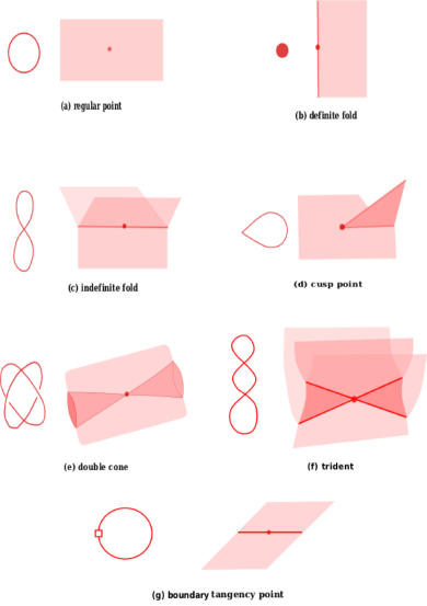
Figure 2: Regular and singular fiber-components and corresponding local configurations in the Reeb Space. The Jacobi Structures are in red lines in the Reeb Space [47].

For a generic map $f:\mathbb{X}\rightarrow\mathbb{R}^{2}$, $\mathbb{W}_{f}$ is a two-dimensional polyhedron and Jacobi structure embedded in the Reeb Space consists of 1-dimensional components which are at the boundary of the two-dimensional sheets in $\mathbb{W}_{f}$. Now a 1-manifold component of the Jacobi Structure can be classified into three types based on the transition of number of regular fiber-components if one passes across the component [49]:

1. Birth-Death or Boundary component - where a fiber-component takes birth or dies (Figure 2 (b)),

2. Merge-Split component or Bifurcation locus - where two (or more) fiber-components merge together or one component splits into two (or more) (Figure 2(c)) and

3. Neutral component - where there is no change in the number of fiber-components if one passes through such components (Figure 2(g)), but here, the topology of the regular fiber-component changes from a circle to an arc (or vice versa).

A connected component of the Jacobi structure may also consist of a composition of these three types, e.g. in Figure 2(d) the Jacobi structure component consists of a boundary and a merge-split component connected at a discrete cusp point. In Figure 2(e) four merge-split components are connected at a double point on the Jacobi Structure.

Figures 1b and 1e respectively show an example of 8 1-manifold components of the boundary Jacobi Set (red lines in the boundary of the domain) and their corresponding projection in the Reeb Space as 5 1-manifold parts of the Jacobi Structure. From this example, it is clear that a boundary Jacobi Set component may not be the boundary component of the Jacobi Structure in the Reeb Space or vice-versa. In Section 6 we propose an algorithm for computing the Jacobi Structure by constructing a Multi-Dimensional Reeb Graph corresponding to a multi-field.

4.3 Regular and Singular Components

As the number of dimensions increases, the projections of the singular fibers develop more internal structure in the Reeb Space. Consider the Reeb Graph of a scalar function: in this, the projection images of the critical points are single points (0-manifolds) separating edges (1-manifolds). Similarly, for the bivariate fields shown in Figures 1d, 1e and 1f, the projections of the singular fibers are arranged in a Reeb Space along 1-manifold curves which separate 2-manifold sheets. This induces a natural stratification or partition of the Reeb Space into disjoint subspaces (or strata).

To describe a stratification of the Reeb Space and the corresponding domain of the multi-field we first classify the fiber-components of the generic map $f:\mathbb{X}\subseteq\mathbb{R}^{3}\rightarrow\mathbb{R}^{2}$ according to their complexity or codimension of the subspace where they lie [49]. Given the Stein factorization $f=\bar{f}\circ q_{f}$, fiber-components of $f$ can be classified into three classes.

1. $\mathcal{C}^{0}=\{q_{f}^{-1}(s):s\in\mathbb{W}_{f}\text{ and }q_{f}^{-1}(s)\text{ does not contain any }$ $\text{singular point of }f\}$. Fiber-components of this class are the regular fiber-components and their $q_{f}$-images form codimension 0 subspaces in $\mathbb{W}_{f}$, denoted as $\mathbb{W}_{f}^{0}$.

2. $\mathcal{C}^{1}=\{q_{f}^{-1}(s):s\in\mathbb{W}_{f}\text{ and }q_{f}^{-1}(s)\text{ contains exactly one de-}$ $\text{finite or indefinite fold point}\}.$ Singular fiber-components of this class are moderately complex and their $q_{f}$-images form codimension 1 subspaces in $\mathbb{W}_{f}$, denoted as $\mathbb{W}_{f}^{1}$.

3. $\mathcal{C}^{2}=\{q_{f}^{-1}(s):s\in\mathbb{W}_{f}\text{ and }q_{f}^{-1}(s)\text{ contains a cusp point}$ $\text{or two indefinite fold points}\}.$ Singular fiber-components of this class are the most complex and their $q_{f}$-images form codimension 2 subspaces in $\mathbb{W}_{f}$, denoted as $\mathbb{W}_{f}^{2}$.

Complexity of a fiber-component increases as the codimension of the corresponding subspace in the Reeb Space increases. Note that $q_{f}$-images of the fiber-components in $\mathcal{C}^{1}$ and $\mathcal{C}^{2}$ form the Jacobi Structure $\mathfrak{J}_{f}$ of the Reeb Space, i.e., $\mathfrak{J}_{f}=\mathbb{W}_{f}^{1}\cup\mathbb{W}_{f}^{2}$. Topologically, regular fiber-components are either a circle or an arc [47]. For stable maps $f:\mathbb{X}\subseteq\mathbb{R}^{3}\rightarrow\mathbb{R}^{2}$, topologically there are $7$ different types of singular fibers in $\mathcal{C}^{1}$ and $21$ different types of singular fibers in $\mathcal{C}^{2}$ [47].

Two regular points $a,\,b\in\mathbb{W}_{f}^{0}$ are topologically equivalent in the Reeb Space $\mathbb{W}_{f}$ or $a\sim_{\rho}b$ if there exists a path between $a$ and $b$ without intersecting the Jacobi Structure $\mathfrak{J}_{f}$. It is not difficult to check that ‘$\sim_{\rho}$’ is an equivalence relation. Therefore, the equivalence relation ‘$\sim_{\rho}$’ partitions the regular points of $\mathbb{W}_{f}$ into a set of equivalence classes. Now we prove that each such equivalence class is a 2-dimensional sheet.

Lemma 4.2 (Partition).

The Jacobi structure $\mathfrak{J}_{f}$ of a Reeb space $\mathbb{W}_{f}$ corresponding to a smooth stable map $f:\mathbb{X}\subseteq\mathbb{R}^{3}\rightarrow\mathbb{R}^{2}$ separates the Reeb Space into a set of $2$-manifold components.

Proof. Let $D$ be a small disk in the range consisting of regular values (i.e., $D$ does not intersect $f(\mathbb{J}_{f})$). Then, by Ehresmann’s fibration theorem, $f$ restricted to $f^{-1}(D)$ is equivalent to the projection $D\times F\rightarrow D$, where $F$ is a 1-dimensional compact manifold. So, this means that $q_{f}(f^{-1}(D))$ can be identified with a disjoint union of some copies of $D$, where the number of copies is the same as the number of connected components of $F$. Even when $D$ intersects with $f(\mathbb{J}_{f})$, if we restrict $f$ to the components of the inverse image $f^{-1}(D)$ that do not intersect $\mathbb{J}_{f}$, then the same consequence holds. So, the regular sheets of $\mathbb{W}_{f}$ are locally homeomorphic to $D$, and hence is a 2-manifold. $\Box$

Thus we have the following definition of regular components.

Definition 4.2.

A path-connected component of $\mathbb{W}_{f}\setminus\mathfrak{J}_{f}$ or $\mathbb{W}_{f}^{0}$ is called a regular component.

Generically, the $0$-dimensional strata are in the boundary of the $1$-dimensional strata in the $\mathfrak{J}_{f}$. Therefore, an equivalence relation on the set of points in $\mathbb{W}_{f}^{1}$ can be defined, similarly, where two points of $\mathbb{W}_{f}^{1}$ are equivalent if there exists a continuous path between them without crossing the $0$-dimensional strata in $\mathfrak{J}_{f}$ and each such equivalence class will be considered as a 1-singular component.

Definition 4.3.

A path-connected component of $\mathfrak{J}_{f}\setminus\mathbb{W}_{f}^{2}$ or $\mathbb{W}_{f}^{1}$ is called a 1-singular component.

Note that a 1-singular component in $\mathbb{W}_{f}$ may be an arc or a circle. An arc 1-singular component will also be called as an edge.

Definition 4.4.

Each component of $\mathbb{W}_{f}^{2}$ is called a 0-singular component.

To extract a skeleton graph from the Reeb Space we need adjacency of these regular and 1-singular components which are defined as follows.

Definition 4.5.

1. A circle 1-singular component is self-adjacent (adjacent to itself).

2. If two end points of an arc 1-singular component coincide, then the 1-singular component is self-adjacent.

3. Two distinct 1-singular components $S_{1},\,S_{2}$ are adjacent if $\exists$ a 0-singular component $\alpha_{0}$ such that $S_{1}~{}\cup~{}S_{2}~{}\cup~{}\alpha_{0}$ form a connected space.

Definition 4.6.

A 1-singular component $S_{i}$ is adjacent to a regular component $R_{j}$ if $S_{i}\cup R_{j}$ forms a connected space.

Next we define a connectivity graph of regular and singular components based on their adjacency.

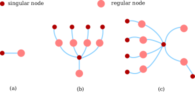
Figure 3: Reeb Skeletons: (a) corresponding to the Reeb Space in Figure 1d, (b) corresponding to the Reeb Space in Figure 1e, (c) corresponding to the Reeb Space in Figure 1f.

4.4 Reeb Skeleton

Once the Reeb space $\mathbb{W}_{f}$ is split into $2$-manifold regular components and $1$-or-lower manifold singular components, it is possible to perform a further reduction from the Reeb Space. To do so, we represent both these regular and 1-singular components as points (or nodes), and add edges representing their adjacency: in short, we can build the dual graph of these components of the Reeb Space. This has the merit of further reducing the Reeb Space from a $2$-dimensional structure to a fundamentally $1$-dimensional structure which is easier to represent, to reason about and to visualise. We refer to this as the Reeb Skeleton and formally define as follows.

Definition 4.7.

Let $R_{1},R_{2},\ldots,R_{m}$ be the regular components and $S_{1},S_{2},\ldots,S_{n}$ be the 1-singular components of $\mathbb{W}_{f}$. Then the Reeb Skeleton of $f$, denoted by $\mathbb{K}_{f}$, is the adjacency graph which consists of (i) nodes $n_{R_{i}}$ and $n_{S_{j}}$ ($i=1,2,\ldots,m$ and $j=1,2,\ldots,n$) corresponding to each of the regular and 1-singular components, and (ii) edges $e(S_{j},S_{j^{\prime}})$ and $e(R_{i},S_{j})$ that are defined as follows:

1. If $S_{j}$ is self-adjacent, then $e(S_{j},S_{j})=1$. In other words, $n_{S_{j}}$ has a self-loop.

2. If $S_{j}$ is self-adjacent and $S_{j}$ is adjacent with a regular component $R_{i}$, then $e(R_{i},S_{j})=2$. In other words, $n_{S_{j}}$ is connected with $n_{R_{i}}$ by two edges.

3. If $S_{j}$ and $S_{j^{\prime}}$ are two distinct non-boundary 1-singular components, then

   $$e(S_{j},S_{j^{\prime}})=\left\{\begin{array}[]{ccc}1,&\text{ if }S_{j},\,S_{j^{\prime}}\text{ are adjacent}\\ 0,&\text{ otherwise.}\end{array}\right.$$

4. For any regular component $R_{i}$ and any 1-singular component $S_{j}$

   $$e(R_{i},S_{j})=\left\{\begin{array}[]{ccc}1,&\text{ if }R_{i},\,S_{j}\text{ are adjacent}\\ 0,&\text{ otherwise.}\end{array}\right.$$

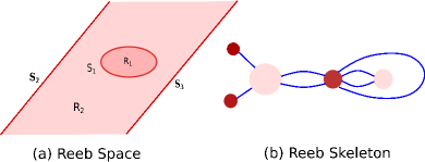
Figure 4: (a) Reeb Space with self-adjacent 1-singular component (b) Corresponding Reeb Skeleton.

The regular and 1-singular components of the Reeb Space are represented as the regular and singular nodes, respectively, in the Reeb Skeleton. Figure 3 shows some examples of Reeb Skeletons corresponding to the Reeb Spaces in Figure 1. Figure 4 illustrates an example of the Reeb Skeleton with a self-adjacent singular node. Note that although the Reeb Skeleton gives a simple abstraction of 0-connectivity in the Reeb Space, it loses information of higher-dimensional connectivities, like higher dimensional holes (tunnels, voids) in the Reeb Space. But on the other hand, the Reeb Skeleton is extremely useful for extracting any “fork”-like structure (corresponding to a merge-split feature) in the Reeb Space. And we will see later by a little simplification we can extract the most prominent merge-split feature in the Reeb Skeleton and so in the Reeb Space. Therefore, next we study properties of the Reeb Skeleton to simplify it further.

4.5 Simple Domains

We know from scalar fields that topologically simple domains have a useful property: the Reeb Graph is guaranteed to be a tree - i.e. the contour tree. This not only enables more efficient computation, but also provides straightforward mechanisms for feature extraction, simplification and visualisation. Ideally, in multi-fields, the Reeb Space would also be contractible to a point. But we show this is not true, in general.

In topology, simple domains are characterised by simply-connected space. A topological space is simply-connected if it is path-connected and every loop in that space can be continuously shrunk to a point without leaving the space. In terms of homotopy theory this means a simply-connected space is without any “handle-shaped hole” (as in Figure 5) or it has trivial fundamental group. For example, a sphere (that has a hollow center) is a simply-connected space whereas a torus (that has a handle-shaped hole) is not. Even a simpler topological space is known as contractible space which is homotopically equivalent to a point. Note that a contractible space is simply-connected, but the converse is not true. For example, a sphere is simply-connected as every loop on it can be contracted to a point on it, although the sphere is not a contractible space because of the center hole in it. In the following lemma, we prove that the Reeb Space corresponding to a map defined on a simply-connected domain is simply-connected, but later we show it may not be contractible.

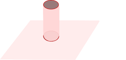
Figure 5: Example of Reeb Space with a tunnel.

Lemma 4.3 (Simply-Connected).

The Reeb Space of a generic continuous map $f:\mathbb{X}\subseteq\mathbb{R}^{3}\rightarrow\mathbb{R}^{2}$ is simply-connected.

Proof. We consider any loop in the Reeb space $\mathbb{W}_{f}$. Then, it lifts to an arc in $\mathbb{X}$. But, every fiber of $q_{f}$ is connected, and therefore, it lifts to a loop. As $\mathbb{X}$ is simply-connected, this lifted loop is null-homotopic. Therefore, its $q_{f}$-image is also null-homotopic from the continuity of $q_{f}$. This means that $\mathbb{W}_{f}$ is simply-connected. $\Box$

Therefore, if $f$ is good enough (for example, triangulable or piecewise linear), then the Reeb space is simply-connected. This implies that the 1st homology of the Reeb Space also vanishes (or is the trivial group), and therefore the Reeb space does not have a tunnel or $1$-dimensional hole (i.e., a hole inside a circle $S^{1}$, e.g. Figure 5). Thus we have the following theorem.

Theorem 4.4.

The Reeb Space of a generic map $f:\mathbb{X}\subseteq\mathbb{R}^{3}\rightarrow\mathbb{R}^{2}$ does not contain any tunnel or $1$-dimensional hole.

On the other hand, for void or $2$-dimensional hole (i.e., hole inside a sphere $S^{2}$), this is no longer true. We can construct a (piecewise linear) map $f:\mathbb{X}\rightarrow\mathbb{R}^{2}$ whose Reeb space does have a $2$-dimensional hole. For example, consider the Hopf fibration $\mathbb{S}^{3}~{}\rightarrow~{}\mathbb{S}^{2}$ and its composition with a standard projection $\mathbb{S}^{2}~{}\rightarrow~{}\mathbb{R}^{2}$. The resulting map $\mathbb{S}^{3}~{}\rightarrow~{}\mathbb{R}^{2}$ is not generic, but perturbing it slightly along its Jacobi set, we can obtain a generic map $\mathbb{S}^{3}~{}\rightarrow~{}\mathbb{R}^{2}$, whose Reeb space is the union of a $2$-sphere and an annulus attached along the equator (and one boundary component of the annulus). Then, by extracting a 3-ball in the preimage of a two disk in the interior of the annulus part, we get the desired map $\mathbb{X}~{}\rightarrow~{}\mathbb{R}^{2}$. The Reeb space is the same space; the union of $\mathbb{S}^{2}$ and an annulus (Figure 6). Over each blue point lies a point (definite fold) and it corresponds to a birth-death. Over each red point lies a fiber as in Figure 2(c) (with an indefinite fold) and the splitting of a circle fiber occurs. Over each green point lies a circle touching the boundary of the domain cube $\mathbb{X}$. Thus, over each point in the shaded disk bounded by the green circle lies an interval. Note this disk is a subset of the annulus part. Therefore, a Reeb Space of a multi-field on a contractible domain may not be contractible and simplification of such space may not be simple as in the scalar case.

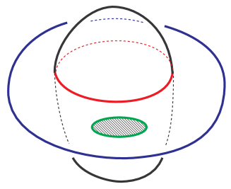
Figure 6: Reeb Space with a void.

According to Theorem 4.4, we can conclude that each regular component of $\mathbb{W}_{f}$ is planar; i.e., each regular component is a disk possibly with holes. For example, torus with holes (or a 1-dimensional hole as in Figure 5) never appears! This is essential in applying our simplification rules for the Reeb Skeleton as will be discussed in Section 6.6 (Figure 11). Next we focus on finding a criterion for detachability of such regular components from the Reeb Space for simplifying the corresponding the multi-field.

4.6 Detachability

In the case of scalar field in a simply-connected domain, the Reeb Space (Graph) is a contour tree and there always exists a leaf edge that can be detached in a mathematically correct way, unless the contour tree consists only of one edge. We find similar criteria for defining detachable regular components in the Reeb Space.

We say that it is possible to detach a regular component from a Reeb Space to obtain a simplified Reeb Space if the multi-field corresponding to the initial Reeb Space could be simplified to the multi-field corresponding to the modified one, and then the regular component is said to be detachable from the Reeb Space. Mathematically, any map could be simplified to a simpler map in the following sense. Since $\mathbb{R}^{2}$ is contractible, any two stable maps $f_{0}$ and $f_{1}:\mathbb{X}\rightarrow\mathbb{R}^{2}$ are homotopic. So, using singularity theory, we can show that $f_{0}$ and $f_{1}$ are connected by a generic 1-parameter family of maps. So, if we take an arbitrary stable map as $f_{0}$ and a very simple map as $f_{1}$, then $f_{0}$ is simplified to $f_{1}$ after the generic 1-parameter family. Such a 1-parameter family passes through finitely many bifurcation parameters, and such bifurcations can be classified [38].

Such transitions of the Reeb Spaces for generic smooth maps on a closed 3-dimensional manifold into $\mathbb{R}^{2}$ have been studied in [38], although for maps on a 3-dimensional manifold with boundary these results need further extension. In the current paper, we consider only a simple type of singularities and show that corresponding regular component is detachable from the Reeb Space. These components are known as lips and are defined as follows.

Definition 4.8.

A lip is a regular component that is attached to the other sheets of the Reeb Space exactly along one edge or an arc 1-singular component, and it should not contain any vertex on the boundary, except for the two cuspidal points (Figure 7(a)).

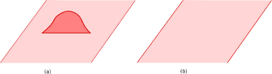
Figure 7: Lip simplification: (a) Reeb Space with a lip, (b) Simplified Reeb Space.

Next we prove the following lemma to show that the underlying map corresponding to a lip can be simplified.

Lemma 4.5.

For a generic bivariate field $f:\mathbb{X}\subseteq\mathbb{R}^{3}\rightarrow\mathbb{R}^{2}$, a “lip” can always be detached safely.

Proof. If we have a lip in the Reeb Space, there are three possibilities as shown in Figure 8. That is, we may consider the map near the inverse image of the lip as a 1-parameter family of functions on a piece of surface. Let $S_{0}$ be a “piece of surface” (a cylinder or a square as in Figure 8), and $f_{t}:S_{0}\rightarrow\mathbb{R},\,t\in\mathbb{I}$, be the 1-parameter family of height functions as in Figure 8. Then, the original map $f$ is equivalent to the map $(x,t)\rightarrow(f_{t}(x),t)$, $x\in S_{0},\,t\in\mathbb{I}$, around the inverse image of a neighborhood of the lip by $q_{f}$. The Figure 8 presents the three such families of functions. As we can see easily, these can be eliminated continuously, by just shrinking the “time interval” for which a pair of critical points appear.

Figure 8: The behavior of the stable map near the pre-image of a neighborhood of the lip. The red lines indicate the boundary of the domain.

$\Box$

Thus, we see that lips are detachable and they can be simplified as in Figure 7. Therefore, we get our simplification rule for detaching the lip components as follows.

Simplification Rule: Let $R_{i}$ be a detachable lip component of the Reeb Space $\mathbb{W}_{f}$. Then we simplify the Reeb Space by (i) deleting $R_{i}$ with its adjacent boundary 1-singular component and (ii) converting the attached arc 1-singular component (merge-split) and two 0-singular components (cusp vertices) as regular.

Next we discuss the Reeb Space (Skeleton) simplification based on the rule developed in this section.

5 Reeb Space Simplification and Measures

In the real multi-field data because of noise very often there are “lip”-like components which occlude the original feature captured by the Reeb Space. Therefore it is important to simplify such components to understand the topology of the underlying data. Given that it is possible to detach such “lip”-like regular components from the Reeb Space, we follow a similar strategy to that used for the contour tree [9]. There, a leaf edge was chosen for pruning and removed from the tree. If as a result a saddle point became regular (i.e. 1-manifold), it too was removed, simplifying the graph further. By tracking which leaves, saddles and edges are removed, the branch decomposition [42] then gave a natural simplification hierarchy for any ordering of leaves.

In any Reeb space where Lemma 4.5 applies, we can use the same strategy, building a simplification hierarchy in the process. To do so, we simply choose a detachable component and remove it from the Reeb Space as described in the simplification rule of Section 4.6. We illustrate this process in Figure 12, where we progressively remove detachable regular components from the Reeb Space, reducing the Jacobi Structure accordingly as much as desired. As in leaf-pruning of contour trees, “lip”-simplification reduces the number of regular components in the Reeb Space by one each time, and also remove components of the Jacobi Structure, guaranteeing that the number of steps required is linear in the number of regular components of the Reeb Space. Moreover, the editing operations to update the Reeb Space, Jacobi Structure and Reeb Skeleton are constant at every step, making the simplification effectively linear (in the number of regular components) once the order of reduction is known. Therefore, we study different measures to associate with the regular components (nodes) of the Reeb Space (Skeleton).

5.1 Range Measure

In simplifying the contour tree, Reeb Graph and Morse-Smale Complex, simplification can be defined by cancelling pairs of critical points according to an ordering given by a filtration - i.e. a sequence by which simplices are added to a complex. For any given filtration, a unique ordering exists, and the persistence of a feature is defined by the distance in the filtration between the critical points defining the feature.

For scalar data, however, the order in the filtration is dictated by the isovalues associated with each vertex of the simplex, with the result that persistence can also be formalised as the isovalue difference between the critical points that cancel each other. In multi-fields, the persistence of a feature gives rise to tuples rather than a single value [5], which does not naturally give rise to a total ordering of the features.

This is however, not the only way to define a simplification ordering. Carr et al. [9] showed that pruning leaves individually could be ordered by geometric properties such as area, volume etc. of the features defined by the contour tree. In this model, persistence is the vertical height of a feature corresponding to a branch of the contour tree, and removing leaves can be done with simple queue-based processing. Recently, Duffy et al. [14] demonstrated that many properties of isosurfaces in scalar and multi-fields relate to geometric measure theory. In this model, statistical and geometric properties of a function are measured by integration over the range. Following a similar approach we introduce a range measure for computing area of the regular components using the induced measure from the range to the Reeb Space. Note that, in general a regular component of a Reeb Space is projected to the range with multiplicities: i.e., this map is an immersion, but may not be injective.

Consider for example the Reeb spaces shown in Figure 1 for bivariate volumetric maps. Mathematically, range measure of a regular component in the Reeb space $\mathbb{W}_{f}$ is defined as the area of the 2-dimensional sheets with respect to the measure induced from the usual area measure of the range Euclidean space. The range measure of each regular component in the Reeb space is a fixed scalar value. Thus, there is a unique induced ordering for simplification. If two components have identical range measure, some form of perturbation will be required to guarantee a strict ordering.

5.2 Geometric Measures

Similarly, it is also possible to compute geometric properties of the regular components, either in the domain, in the range, or in some combination of the two, using geometric measure theory. As with the contour tree [9], obvious properties of interest include the measure of the region’s boundary in the domain (contour length in 2D, isosurface surface area in 3D), the measure of the region in the domain (area in 2D, volume in 3D), the measure of the function over the region (a generalisation of the volume in 2D, hypervolume in 3D), and so forth. However, as in that work, rules will be needed in each case for combination of measure with parents in the simplification hierarchy based on the theory in Section 4.6.

5.3 Summary of Theoretical Contributions

We have now completed the theoretical groundwork for practical simplification algorithm of Reeb Spaces. In particular our theoretical results could be summarised as follows.

1. The Reeb Space consists of regular components corresponding to regions in the domain of the function, and singular components describing their relationships.

2. The Jacobi Set in the domain does not capture all of the structure of the singular components in the Reeb Space, and the Jacobi Structure is needed to do so.

3. The Jacobi Structure of the Reeb Space can be used to further collapse the Reeb Space into the Reeb Skeleton.

4. Multifields with topologically simple domains can be simplified using a variation on the leaf-pruning used for contour trees.

5. A Reeb Space measure and other geometric measures are introduced to guide the Reeb Space simplification process.

We now turn to the practical and algorithmic part of this paper: how to simplify the Joint Contour Net, an approximation of the Reeb Space.

Figure 9: (top) The joint contour fragments and their adjacency graph for a PL-bivariate field defined by the values $\{(5,0),(0,0),(5,0),(3,2)\}$ at the vertices of a mesh of two triangles. (middle) The Multi-Dimensional Reeb Graph constructed from the JCN. The critical nodes of the MDRG are the ‘red’ nodes which form the Jacobi Structure. (bottom) Corresponding Joint Contour Net, with critical nodes from the MDRG marked in colour.

6 Algorithm: Simplifying the Joint Contour Net

In this section, first we introduce the Joint Contour Net, a graph data-structure that approximates the Reeb Space. As described in [7], the Joint Contour Net is a quantized approximation of the Reeb Space. Therefore, to avoid having duplicate terminology we will use the same terminology for JCN as what we have developed for the Reeb Space, namely, Jacobi Structure, Regular Component, Singular Components, Reeb Skeleton etc.

6.1 Joint Contour Net

The Joint Contour Net (JCN) [7, 15] approximates the Reeb Space $\mathbb{W}_{f}$ of a multi-field $f=(f_{1},\,f_{2},\,\ldots,\,f_{r}):\mathbb{X}\subset\mathbb{R}^{d}\rightarrow\mathbb{R}^{r}$ in a $d$-dimensional interval $\mathbb{X}$. Let $\tilde{f}=(\tilde{f}_{1},\,\tilde{f}_{2},\,\ldots,\,\tilde{f}_{r}):M\rightarrow\mathbb{R}^{r}$ be a piecewise-linear (PL) approximation of $f$ corresponding to a mesh $M$ of $\mathbb{X}$. The idea of computing the JCN is based on quantization of the fiber-components of $\tilde{f}$. The JCN $\tilde{f}$ with a quantization level (or level of resolution) $m_{Q}$ is denoted as $JCN(\,\tilde{f},m_{Q})$, where $m_{Q}$ refers to how fine the rectangular mesh for the range is.

A quantized level set of $\tilde{f}_{i}$ at an isovalue $h\in\mathbb{Z}/m_{Q}$ is denoted by $Q\tilde{f}_{i}^{-1}(h)$ and is defined as: $Q\tilde{f}_{i}^{-1}(h):=\big{\{}x\in M:(\frac{1}{m_{Q}})\operatorname{round}(m_{Q}\tilde{f}_{i}(x))=h\}$. A connected component of the quantized level set in the mesh is called a quantized contour or a contour slab. The part of the contour slab in a single cell of the mesh is called a contour fragment.

Now the first step of the JCN algorithm constructs all the contour fragments corresponding to a quantization of each component field. In the second step, the joint contour fragments are computed by computing the intersections of these contour fragments for the component fields in a cell. The third step is to construct an adjacency graph of these joint contour fragments where a node in the graph corresponds to a joint contour fragment and there is an edge between two nodes if the corresponding joint contour fragments are adjacent. Finally, the JCN is obtained by collapsing the neighbouring redundant nodes with identical isovalues. Thus, each node in the JCN corresponds to a joint contour slab (or quantized fiber-component) and an edge represents the adjacency between two quantized fiber-components (with quantization level $m_{Q}$) of $\tilde{f}$.

Note that one can build a multi-resolution JCN by increasing or decreasing the quantization level using a scaling factor for the ranges of the component fields. An example of a small JCN is given in Figure 9, but we refer the interested reader to [7] for details. The following lemma shows that in the limiting case, when the quantization level increases and the domain-mesh becomes more refined, then the JCN converges to the corresponding Reeb Space.

Lemma 6.1 (Convergence).

Let $f:\mathbb{X}\subset\mathbb{R}^{d}\to\mathbb{R}^{r}$, $d\geq r$, be a tiangulable continuous multi-field with the Reeb space $\mathbb{W}_{f}$. Choose an increasing sequence of quantization levels $\{m_{Q}^{(n)}\}$ for $f$ such that $m_{Q}^{(n)}$ is an integer multiple of $m_{Q}^{(n-1)}$ for each $n$ and $\displaystyle\lim_{n\to\infty}m_{Q}^{(n)}=\infty$. Furthermore, let $\{M_{n}\}$ be sequence of sufficiently fine meshes of $\mathbb{X}$ such that $M_{n}$ is a refinement of $M_{n-1}$ for each $n$ and $\displaystyle\lim_{n\to\infty}d(M_{n})=0$, where $d(M_{n})$ stands for the maximum of the diameters of the cells of $M_{n}$. Finally, let $f^{(n)}:M_{n}\to\mathbb{R}^{r}$ be the PL map associated with $f$ corresponding to the mesh $M_{n}$. Then the sequence $\left\{JCN(\,f^{(n)},m_{Q}^{(n)})\right\}$ converges to $W_{f}$.

Proof. Hiratuka et al. [27] show for a PL map $f:A\to B$ of a compact polyhedron $A$ into another polyhedron $B$, if we subdivide the range polyhedron $B$ appropriately, then $A$ is subdivided accordingly and the quotient map $q_{f}:A\to\mathbb{W}_{f}$ to the Reeb Space $\mathbb{W}_{f}$ is triangulable with respect to the triangulations. In the proof, it is also shown that the inverse image by $q_{f}$ of a small regular neighborhood of a vertex $v$ in $\mathbb{W}_{f}$ is always a regular neighborhood of $(q_{f})^{-1}(v)$ in $A$. This implies that if the quantization level is high enough, then the quantized fiber-component is actually a regular neighborhood of the central fiber-component. Consequently, we have a natural embedding $\rho_{0}:JCN_{0}^{(n)}\to\mathbb{W}_{f}$, where $JCN_{0}^{(n)}$ is the set of vertices of the Joint Contour Net $JCN(\,f^{(n)},m_{Q}^{(n)})$ for sufficiently large $n$. (For each quantized fiber-component, associate the central fiber-component.) Furthermore, as is shown in [27], this embedding preserves the adjacencies. This implies that the embedding $\rho_{0}$ extends to an embedding $\rho:JCN(\,f^{(n)},m_{Q}^{(n)})\to\mathbb{W}_{f}$. Hence, the required result holds, since the triangulations of $JCN(\,f^{(n)},m_{Q}^{(n)})$ and $\mathbb{W}_{f}$ becomes finer and finer as $n$ increases.

If $f$ itself is not a PL map, then we can consider its triangulation $g:A\to B$ and obtain the required result for the triangulation. As the domain $\mathbb{X}$ is compact, this implies the same consequence for the original map $f$ as well. This completes the proof. $\Box$

Next we see that the simplification will have four stages: 1. extraction of the Jacobi Structure from the JCN, 2. computing regular and singular components for construction of the Reeb Skeleton, 3. computation of measures for each regular node in the Reeb Skeleton, and 4. simplification by pruning nodes corresponding to the “lip” components. In practice, the first stage is the most difficult - identifying the regular components, and this requires an intermediate data-structure, which we introduce now.

6.2 Multi-Dimensional Reeb Graphs

The first step in detecting and analysing the Jacobi Structure is to identify the nodes in the JCN that capture changes in the topology - i.e. the quantized representatives of the Jacobi Structure. To do so, we exploit a simple property of the JCN - that the slabs can be arranged hierarchically, with the levels of the hierarchy corresponding to the individual fields. At the highest level of the hierarchy, the slabs are only defined by field $f_{1}$, and are therefore equivalent to interval volumes: as such, we can compute the Reeb Graph for field $f_{1}$ (see Figure 9 (middle)).

Algorithm 1 CreateReebGraph$(G,f_{i})$

Input: A subgraph $G$ of $JCN$ and a chosen field $f_{i}$
Output: The Reeb Graph $RG$ with respect to field $f_{i}$

1:Create Union-Find Structure $UF$ for field $f_{i}$.

2:For each adjacent $g_{1},g_{2}\in G$ with $f_{i}(g_{1})=f_{i}(g_{2})$, UFAdd($g_{1},g_{2})$

3:for  each component $C_{l}$ in UF do

4:     Create a node $n_{C_{l}}$ in $RG$

5:     Map graph node-id(s) and field-values from $G$ to $n_{C_{l}}$

6:end for

7:Order nodes ${n_{C_{1}},\ldots,n_{C_{n}}}$ according to $f_{i}$ field values.

8:for edge $e_{1}e_{2}$ in $G$ do

9:     if $e_{1},e_{2}\in$ components $C_{j}\neq C_{k}$ and $f_{i}(e_{1})\neq f_{i}(e_{2})$ then

10:         Add edge $e(n_{C_{j}},n_{C_{k}})$ in $RG$ if not already present

11:     end if

12:end for

13:return $RG$

Each slab (i.e. interval volume) of $f_{1}$ can be broken up into smaller slabs with respect to field $f_{2}$ in a similar way (which form a subgraph $G$ in the JCN), and the Reeb graph for these slabs computed similarly, as shown in Algorithm 1. Proceeding recursively, we then compute a hierarchy of Reeb graphs, each of which represents the internal topology of a slab of the parent Reeb Graph with respect to the child’s field. We call this hierarchy the Multi-Dimensional Reeb Graph or MDRG and denote this as $\mathbb{M}_{f}$.

Computing the MDRG is straightforward once the full JCN has been extracted: we start with the JCN and compute the Reeb Graph for property $f_{1}$ by performing union-find processing over the nodes of the JCN. This breaks the JCN into subgraphs corresponding to slabs in the Reeb Graph of property $f_{1}$. The MDRG for each subgraph is then computed recursively, and stored in the node of the parent Reeb Graph to which its slab corresponds. In the process, the slabs get separated out into smaller and smaller components.

Algorithm 2 MultiDimensionalReebGraph$(G,f_{i},\ldots,f_{r})$

Input: Graph $G$, fields $f_{i},\ldots,f_{r}$ Output: MDRG $M$

1:if $i\leq r$ then

2:     Let $R=$ CreateReebGraph($G,f_{i}$)

3:     Store $R$ as root node of $M$

4:     for Each slab $s$ of $R$ do

5:         Extract subgraph $G_{s}$ of nodes of $G$ belonging to $s$ in $R$

6:         Compute $M_{s}=$ MultiDimensionalReebGraph($G_{s},f_{i+1},\allowbreak\ldots,f_{r}$)

7:         Store $M_{s}$ at node $s$ of $R$

8:     end for

9:     return $M$

10:else

11:    return $M=\emptyset$

12:end if

We state this as an algorithm in Algorithm 2 and illustrate with a bivariate field in Figure 9. This algorithm is stated recursively for simplicity, but can also be implemented with queue processing for speed. Moreover, the division of subgraphs at each level into slabs can be performed more efficiently by exploiting the connectivity already encoded in the JCN.

The principal value of the MDRG is that every node of the JCN in the Jacobi Structure is guaranteed to be a critical node of the finest-resolution Reeb Graphs (denoted as the critical nodes of the MDRG). This immediately gives a method of computing the Jacobi Structure once the MDRG is known [10].

6.3 Jacobi Structure Extraction

Since every node belonging to the Jacobi Structure is guaranteed to appear as a critical node of the lowest level of an MDRG, the initial stage in Jacobi Structure extraction is simply to mark these nodes. Unmarked nodes are then guaranteed to be regular, and can be collected into regular components. Once this has been done, any remaining nodes that are adjacent to each other and to the same set of regular components are identified, as these form a 1-singular component between the regular components.

The first stage of this can be seen in Figure 9, where the critical nodes of the lowest level of the MDRG together mark all of the Jacobi Structure nodes in the JCN (in colour).

6.4 Reeb Skeleton Construction

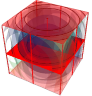
(a)

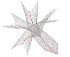
(b)

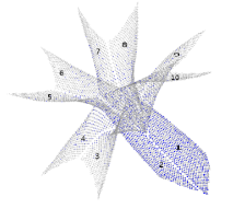
(c)

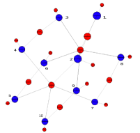
(d)

Figure 10: (a) Bivariate Field: $(x^{2}+y^{2}-z$, $x^{2}+y^{2}+z^{2})$ in a box $[-5,\,5]^{3}$, the ‘red’ components are the Jacobi Set, (b) the Joint Contour Net with the Jacobi Structure (in red), (c) Regular Components, (d) the Reeb Skeleton.

Once we have extracted the Jacobi Structure for the JCN, it is straightforward to compute the corresponding Reeb Skeleton by creating a single node for each regular or 1-singular component, and connecting them using the adjacency of components in the Jacobi Structure. In Figure 10 we see an example of the Reeb Skeleton construction for a volumetric bivariate field. We note, in this case, the Reeb Skeleton has no detachable lip-like regular node whereas the Reeb Skeleton Figure 12 (d) has such detachable nodes.

Now in the simplification algorithm, the order in which detachable Reeb Skeleton nodes are removed is determined by the metrics associated with those nodes. Computation of such metrics are described next.

Algorithm 3 SimplifyReebSpace

Input: JCN $JCN$ 
Output: Reeb Skeleton $\mathbb{K}_{f}$

1:Build MDRG $\mathbb{M}_{f}$ and Jacobi Structure $\mathfrak{J}_{f}$ from JCN $JCN$ .

2:Partition $JCN$ into disjoint regular components $C=\{R_{1},\ldots,R_{m}\}$ by deleting $\mathfrak{J}_{f}$ from $JCN$ .

3:Partition $\mathfrak{J}_{f}$ into disjoint 1-singular components $\{S_{1},\ldots,S_{n}\}$ based on adjacency to regular components in $C$.

4:Use adjacencies of $\{R_{1},\ldots,R_{m},S_{1},\ldots,S_{n}\}$ to construct $\mathbb{K}_{f}$ (following defintion 4.7).

5:Push “detachable” nodes of $\mathbb{K}_{f}$ on priority queue $PQ$ with priority determined by geometric measures.

6:while $PQ$ not empty (or priority is below a threshold value) do

7:     Pop node $r$ from queue

8:     Prune $r$ from $\mathbb{K}_{f}$

9:end while

10:return Simplified Reeb Skeleton $\mathbb{K}_{f}$.

6.5 Computing Simplification Metrics

Our simplification algorithm can use any desired measure of importance for components of the Reeb space, including but not limited to:

• Range measure. As described in Subsection 5.1, we can measure the size of the regular components by the induced measure of the range. This is easy to approximate - in this case, by the number of unique JCN slabs (i.e. pixels in the range) that map to a given regular component.

• Surface area. A regular component of the Reeb space is separated from other regular components by one or more singular components in the Jacobi Structure. Since the regular components correspond to features and the singular components to boundaries between features, we can associate the area of the bounding surface with the regular component for the purpose of simplification. For the JCN, we can approximate this with the surface area of the fragments adjacent to the bounding region.

• Volume. Similarly, we can measure volume in the domain for each feature represented by a regular component, and approximate it by summing the volume of fragments mapping to a given regular component.

• Other measures. As shown by Duffy et al. [14] and Carr et al. [9], almost any geometric or other property of features can be used for simplification provided that it is correctly approximated and suitable rules for composition during simplification are established.

6.6 Simplifying the Reeb Skeleton

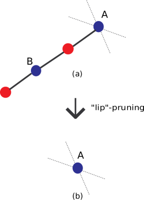
Figure 11: Simplification rule for detaching a lip-like node (regular node B in (a)) from the Reeb skeleton.

The lip-simplification rule of the Reeb Space, as described in Section 4.6, can be translated similarly in the corresponding Reeb Skeleton. We note, according to Theorem 4.4, each regular component of our Reeb Space is always a disk possibly with holes. Therefore, the degree 2 regular node B as in a Reeb Skeleton Figure 11(a) is always a lip-like detachable node. Figure 11(b) shows the simplified Reeb Skeleton after pruning the lip-like node and attached singular nodes.

Finally, we give simplification strategies of the Reeb Skeleton, based on geometric and range measures of the components. The Reeb skeleton simplification method simplifies the Reeb skeleton and the corresponding Reeb space given a threshold (between 0 and 1) adapting the previous approaches in the literature [6, 54]. The threshold represents a “scale”, under which detachable regular nodes of the Reeb skeleton are considered as unimportant (noise). The threshold is expressed as a fraction of the range of the metric used. It can vary from 0 (no simplification) to 1 (maximal simplification).

Figure 12 demonstrates the simplification of components from the Reeb Space, of an unstable bivariate volumetric data. We use range measure for ordering the components. We note, regular nodes 4 and 2 in Figure 12 are not strictly the lips according to our definition of lips. However, a perturbation can be applied first to convert such components to lips and then lip simplifications can be applied. In Figure 12 we apply our lip-simplification rule directly at the regular nodes 4 and 2, sequentially (node with smaller measure is pruned first).

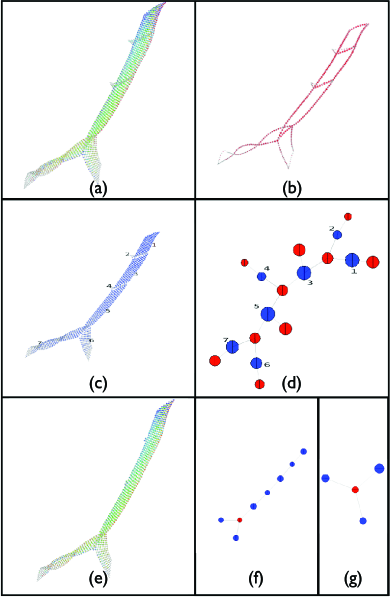
Figure 12: (Simplification Demo) (a) Original JCN/Reeb Space of bivariate field (Paraboloid, Height) (b) Jacobi Structure, (c) Regular components (d) Reeb Skeleton (‘blue’ corresponds to regular components and ‘red’ corresponds to adjacent 1-singular components) (e) Simplified JCN (f)-(g) Simplified Reeb Skeleton using range measure.

7 Implementation and Application

We implement our Reeb Space or JCN simplification algorithm using the Visualization Toolkit (VTK) [1]. Details of the JCN implementation can be found in [7, 15]. Our Reeb Space simplification implementation takes the JCN (a vtkGraph structure) as input and builds four filters: (1) The first filter computes the Jacobi Structure by implementing the Multi-dimensional Reeb graph algorithm, (2) The second filter builds the Reeb Skeleton structure by partitioning the JCN, (3) The third filter implements persistence and geometric measures and (4) The fourth filter implements the simplification rules of the Reeb Skeleton. We use a vtkTree structure to store the Multi-Dimensional Reeb Graph (MDRG): Reeb graphs at each level of MDRG are stored in a vtkReebGraph structure. For capturing the Reeb skeleton we use the vtkGraph structure.

Table 2: Data Statistics

datasets	spatial-dimensions	slab widths	no. of nodes (JCN)	no. of edges (JCN)
(Circle, Line)	(29, 29, 1)	(1, 1)	500	1057
(Paraboloid, Height)	(40, 40, 40)	(1, 1)	1260	2383
(Sphere, Height)	(40, 40, 40)	(1, 1)	1308	2428
(Paraboloid, Sphere)	(40, 40, 40)	(1, 1)	6554	12795
(Cubic, Height)	(40, 40, 40)	(1, 1)	3149	5928

A force-directed graph-layout from the OGDF - an Open Graph Drawing Framework [11] strategy has been used for the graph visualization as shown in the demonstrations and outputs. We run our implementation on different synthetic and simulated data sets for testing the performance. In Table 2 the synthetic data sets are labelled by the combination of scalar fields used: Circle: $x^{2}+y^{2}$, Line: $y$, Sphere: $x^{2}+y^{2}+z^{2}$, Paraboloid: $x^{2}+y^{2}-z$, Height: $z$ and Cubic: $(y^{3}-xy+z^{2},\,x)$. Circle and Line are in the 2D-box $[-5,\,5]^{2}$ and other fields are considered in the 3D-box $[-5,\,5]^{3}$.

Table 3: Performance results for Simplification

Data	Spatial	Slab	Jacobi	Reeb
	Dimensions	Widths	Structure	Skeleton	Simplification
(Circle, Line)	(29, 29, 1)	(1, 1)	0.06s	0.242s	0.00s
(Paraboloid, Height)	(40, 40, 40)	(1, 1)	0.10s	1.97s	0.00s
(Paraboloid, Sphere)	(40, 40, 40)	(1, 1)	0.80s	33.02s	0.00s
Nucleon	(40, 40, 66)	(8,2)	0.45s	48.91s	0.45s

Performance results

Table 3 shows the performance results of the JCN and MDRG algorithms for some simulated data. All timings were performed on a 3.06 GHz 6-Core Intel Xeon with 64GB memory, running OSX 10.8.5, and using VTK 5.10.1.

The number of nodes in the MDRG is actually the number of Reeb graphs computed by the MDRG Algorithm 2. From the table it is clear that performance of the MDRG algorithm is quite impressive for these simulated data. The complexity of the CreateReebGraph on a graph with $n$ nodes is $O(n+p\log n)$ which is the complexity of a sequence of $p$ UF operations (here, $p\leq n$) [53].

Nuclear Scission Data

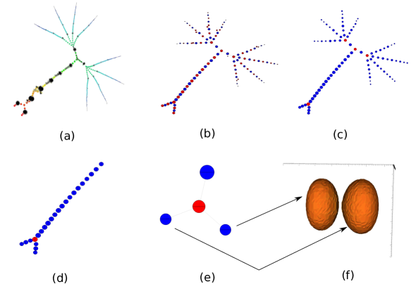
Figure 13: This figure shows the simplification process of the JCN corresponding to a “nuclear scission” data set used in [15]. The process includes: (a) The original JCN graph; (b) The Reeb Skeleton; (c) A modified representation of the Reeb Skeleton by changing the colour of the degree 2 singular nodes as “blue”, since they capture only minor topological information, (d) Simplified Reeb Skeleton after applying lip-pruning using the range measure for ordering the nodes (e) Resultant Reeb Skeleton is represented as the “Y”-fork; (f) Geometry corresponding to the “scission” point.

In a previous application paper [15], the JCN was applied to nuclear data set (time-varying bivariate field of proton and neutron densities) and used to visualise the scission points in high-dimensional parameter spaces. Here the scission refers to the point where a single plutonium nucleus breaks into two fragments. However, this was based on visual analysis, and was complicated by a number of artefacts such as the recurring chains of star-like ‘motifs’ within the JCN. Moreover, the eight corners of the domain boundary induced eight corresponding small sets of features in the JCN.

Here we apply our simplification algorithm to overcome these artefacts and preserve the principal topological feature. Note that apparently there are two red nodes that are adjacent to 5 blue nodes in the Reeb Skeleton Figure 13(b). This never happens if the given multi-field is stable, so this is an example of an unstable bivariate field in 3-dimensional interval. We demonstrate the process of simplification for one of these scission data sets in Figure 13. Note that the final simplification results a simple Y-fork where two regular nodes correspond to the separated nuclei, while the third represents the exterior.

8 Conclusions and Discussions

In this paper, we provide a rigorous mathematical and computational foundation of multivariate simplification based on lip-pruning from its Reeb Space and this generalises approaches that are effective for scalar fields. We note, lip-simplification can be applied only when there is a lip-component in the Reeb Space and might not always be possible, but nevertheless, it is quite effective when applied to real data sets, which usually contain a lof of noise (as demonstrated in Figure 13). The Jacobi Structure that characterises the Reeb Space is richer than the Jacobi Set and decomposes the Reeb Space. This is proved to be a useful property for the simplification procedure. In addition, we have shown how to extract a reliable approximate Jacobi Structure and Reeb Skeleton from the JCN that can be simplified to improve the use of the JCN for multivariate analysis, and illustrated this with analytical datasets and a real-world data. However, there are few open issues which need to be addressed in future research.

• False lips: Currently using our lip simplification approach we are not able to distinguish or simplify the false-lips, similar as in Figure 14. This is because our Reeb Skeleton cannot compute the multiplicity of the adjacency between a regular and a 1-singular node which will be important for detecting such a false lip in the Reeb Space. So, in our current simplification we assume no false lip appears and we can simplify only the “genuine” lips as defined in Definition 4.8.

  
  

  Figure 14: False lip

• Discontinuity in components of Jacobi Structure: Computed 1-singular components of the Jacobi Structure in the JCN may be discontinuous because of the degeneracy, as all degenerate singular points may not be captured by the critical nodes of MDRG. Moreover, a choice of the quantization level may also result in the discontinuous Jacobi Structure in the JCN.

• Further Structures in the Reeb Skeleton: In the current implementation of the Reeb Skeleton we have considered only the regular and the 1-singular components and their adjacency graph. But, there is further hierarchy possible in the Jacobi Structure. For more than bivariate case, singular components can be decomposed into lower dimensional manifolds (strata) and can be represented in the Reeb Skeleton, hierarchically. However, detecting such lower dimensional strata needs further theoretical analysis and an algorithm for detecting them.

Apart from these issues, in the future, we intend to work on further simplification and acceleration of these techniques, and on alternate methods for Reeb Space computation and / or approximation. We also expect to examine more data sets from multiple domains, now that we have solved more of the main theoretical issues.

References

- [1] Visualization Toolkit. http://www.vtk.org/, 2013.
- [2] Harsh Bhatia, Bei Wang, Gregory Norgard, Valerio Pascucci, and Peer-Timo Bremer. Local, Smooth, and Consistent Jacobi Set Simplification. Computational Geometry: Theory and Applications, 48(4):311–332, 2015.
- [3] P-T Bremer, E. M. Bringa, M.A. Duchaineau, D. Laney, A. Mascarenhas, and V. Pascucci. Topological feature extraction and tracking. Journal of Physics: Conference Series, 78:012007, 2007.
- [4] Gunnar Carlsson and Afra Zomorodian. The Theory of Multidimensional Persistence. In SoCG, pages 71–93, 2007.
- [5] Gunnar Carlsson and Afra Zomorodian. The Theory of Multidimensional Persistence. Discrete and Computational Geometry - 23rd Annual Symposium on Computational Geometry, 42(1):71–93, 2009.
- [6] H. Carr, J. Snoeyink, and M. van de Panne. Simplifying Flexible Isosurfaces Using Local Geometric Measures. IEEE Transactions on Visualization and Computer Graphics, 2004.
- [7] Hamish Carr and David Duke. Joint Contour Net. IEEE Transactions on Visualization and Computer Graphics, pages xxx–xxx, 2013. accepted.
- [8] Hamish Carr, Jack Snoeyink, and Ulrike Axen. Computing Contour Trees in All Dimensions. Computational Geometry: Theory and Applications, 24(2):75–94, 2003.
- [9] Hamish Carr, Jack Snoeyink, and Michiel van de Panne. Flexible isosurfaces: Simplifying and displaying scalar topology using the contour tree. Computational Geometry: Theory and Applications, 43(1):42–58, 2010.
- [10] Amit Chattopadhyay, Hamish Carr, David Duke, and Zhao Geng. Extracting Jacobi Structures in Reeb Spaces. In N. Elmqvist, M. Hlawitschka, and J. Kennedy, editors, EuroVis - Short Papers, pages 1–4. The Eurographics Association, 2014.
- [11] Markus Chimani, Carsten Gutwenger, Michael Jünger, Gunnar W. Klau, Karsten Klein, and Petra Mutzel. OGDF - Open Graph Drawing Framework. http://www.ogdf.net/, 2012.
- [12] David Cohen-Steiner, Herbert Edelsbrunner, and John Harer. Stability of Persistence Diagrams. Discrete and Computational Geometry, 37(1):103–120, January 2007.
- [13] Tamal K. Dey, Herbert Edelsbrunner, Sumanta Guha, and Dmitry V. Nekhayev. Topology preserving edge contraction. Publ. Inst. Math. (Beograd) (N.S), 66:23–45, 1998.
- [14] Brian Duffy, Hamish Carr, and Torsten Möller. Integrating Isosurface Statistics and Histograms. IEEE Transactions on Visualization and Computer Graphics, 19(2):263–277, 2012.
- [15] David Duke, Hamish Carr, Nicolas Schunck, Hai Ah Nam, and Andrzej Staszczak. Visualizing nuclear scission through a multifield extension of topological analysis. IEEE Transactions on Visualization and Computer Graphics, 18(12):2033–2040, 2012.
- [16] Herbert Edelsbrunner and John Harer. Jacobi Sets of Multiple Morse Functions. In Foundations of Computational Matematics, Minneapolis, 2002, pages 37–57, 2004. Cambridge Univ. Press, 2004.
- [17] Herbert Edelsbrunner, John Harer, Ajith Mascarenhas, and Valerio Pascucci. Time-varying Reeb Graphs for Continuous Space-Time Data. In Symposium on Computational Geometry, pages 366–372, 2004.
- [18] Herbert Edelsbrunner, John Harer, Vijay Natarajan, and Valerio Pascucci. Local and Global Comparison of Continuous Functions. In Proceedings of the conference on Visualization, pages 275–280, 2004.
- [19] Herbert Edelsbrunner, John Harer, and Amit K. Patel. Reeb Spaces of Piecewise Linear Mappings. In SoCG, pages 242–250, 2008.
- [20] Herbert Edelsbrunner, David Letscher, and Afra Zomorodian. Topological Persistence and Simplification. Discrete and Computational Geometry, 28(4):511–533, 2002.
- [21] Michael Garland and Paul S. Heckbert. Surface simplification using quadric error metrics. In SIGGRAPH, pages 209–216, 1997.
- [22] V. Guillemin and A. Pollack. Differential Topology. Prentice-Hall, Inc., Englewood Cliffs, New Jersey, 1974.
- [23] Igor Guskov and Zoe J. Wood. Topological Noise Removal, 2001.
- [24] Attila Gyulassy, Vijay Natarajan, Valerio Pascucci, Peer-Timo Bremer, and Bernd Hamann. A Topological Approach to Simplification of Three-dimensional Scalar Functions. IEEE Transactions on Visualization and Computer Graphics, 12(4):474–484, 2006.
- [25] Allen Hatcher. Algebraic Topology. Cambridge University Press, 2002.
- [26] Masaki Hilaga, Yoshihisa Shinagawa, Taku Kohmura, and Tosiyasu L. Kunii. Topology Matching for Fully Automatic Similarity Estimation of 3D Shapes. In SIGGRAPH, pages 203–212, 2001.
- [27] J. T. Hiratuka and O. Saeki. Triangulating stein factorizations of generic maps and euler characteristic formulas. RIMS Kôkyûroku Bessatsu, B38:61–89, 2013.
- [28] H.Levine. Classifying immersions into over stable maps of 3-manifolds into . Springer-Verlag, Berlin, 1985. Lecture Notes in Mathematics, 1157.
- [29] Hugues Hoppe. Progressive meshes. In ACM SIGGRAPH 1996 Proceedings, pages 99–108. ACM New York, NY, USA ©1996, 1996.
- [30] Hugues Hoppe, Tony DeRose, Tom Duchamp, John McDonald, and Werner Stuetzle. Mesh optimization. In SIGGRAPH ’93 Proceedings of the 20th annual conference on Computer graphics and interactive techniques, pages 19–26. ACM New York, NY, USA ©1993, 1993.
- [31] L Huettenberger, C Heine, H Carr, G Scheuermann, and C Garth. Towards Multifield Scalar Topology Based on Pareto Optimality. Computer Graphics Forum, 32(3.3):341–350, 2013.
- [32] L Huettenberger, C Heine, and C Garth. Decomposition and simplification of multivariate data using pareto sets. IEEE Transactions on Visualization and Computer Graphics, 20(12):2684–2693, 2014.
- [33] Yi jen Chiang and Xiang Lu. Progressive simplification of tetrahedral meshes preserving all isosurface topologies. Computer Graphics Forum, 22:493–504, 2003.
- [34] L. Kushner, H. Levine, and P. Porto. Mapping Three-Manifolds Into The Plane I. Bol. Soc. Mat. Mexicana, 29(2):11––33, 1984.
- [35] Peter Lindstrom and Greg Turk. Fast and memory efficient polygonal simplification. In IEEE Visualization, pages 279–286, 1998.
- [36] Peter Lindstrom and Greg Turk. Evaluation of memoryless simplification. IEEE Transactions on Visualization and Computer Graphics, 5(2):98–115, 1999.
- [37] C. Luo, I. Safa, and Y. Wang. Approximating gradients for meshes and point cloud via diffusion metric. In In:Proceedings Symposium on Geometry Processing. Eurographics Association, Aire-La-Ville, Switzerland, pages 1497––1508, 2009.
- [38] L.E. Mata-Lorenzo. Polyhedrons and pi-stable homotopies from 3-manifolds into the plane. Bol. Soc. Brasil. Mat. (N.S.), 20:61––85, 1989.
- [39] Xinlai Ni, Michael Garland, and John C. Hart. Fair Morse Functions for Extracting the Topological Structure of a Surface Mesh. ACM Transactions on Graphics (TOG) - Proceedings of ACM SIGGRAPH 2004, 23(3):613–622, 2004.
- [40] Fakir S. Nooruddin and Greg Turk. Simplification and Repair of Polygonal Models Using Volumetric Techniques. IEEE Transactions on Visualization and Computer Graphics, 9(2):191–205, 2003.
- [41] V. Pascucci, P-T Bremer, A. Mascarenhas, and G. Scorzelli. Robust On-line Computation of Reeb Graphs. ACM Transactions on Graphics (TOG), 26(58), July 2007.
- [42] Valerio Pascucci, Kree Cole-McLaughlin, and G. Scorzell. Multi-resolution computation and presentation of contour trees. In Proceedings of the IASTED conference on Visualization, Imaging and Image Processing (VIIP 2004), pages 452–290, 2004.
- [43] Konrad Polthier and Eike Preuß. Identifying Vector Field Singularities using a Discrete Hodge Decomposition. In Mathematical Visualization, Springer-Verlag, New York, pages 113–134, 2003.
- [44] Jovan Popović and Hugues Hoppe. Progressive simplicial complexes. In ACM SIGGRAPH 1997 Proceedings, pages 217–224. ACM New York, NY, USA ©1997, 1997.
- [45] Jan Reininghaus and Ingrid Hotz. Combinatorial 2d Vector Field Topology Extraction and Simplification. Topological Methods in Data Analysis and Visualization, pages 103–114, 2011.
- [46] O. Saeki and T. Yamamoto. Cobordism group of morse functions on surfaces with boundary. Preprint http://imi.kyushu-u.ac.jp/~saeki/research.html#03, 2015.
- [47] O. Saeki and T. Yamamoto. Singular fibers of stable maps of 3-manifolds with boundary into surfaces and their applications. Preprint http://imi.kyushu-u.ac.jp/~saeki/research.html#03, 2015.
- [48] Osamu Saeki. Topology of Singular Fibers of Differentiable Maps. Springer, 2004.
- [49] Osamu Saeki, Shigeo Takahashi, Daisuke Sakurai, Hsiang-Yun Wu, Keisuke Kikuchi, Hamish Carr, David Duke, and Takahiro Yamamoto. Visualizing Multivariate Data Using Singularity Theory, volume 1 of Mathematics for Industry, chapter The Impact of Applications on Mathematics, pages 51–65. Springer Japan, 2014.
- [50] David F. Snyder. Topological Persistence in Jacobi Sets. Technical report, Technical Report July 29, 2004, 2004.
- [51] B Strodthoff and B Jüttler. Layered Reeb graphs for three-dimensional manifolds in boundary representation. Computers & Graphics, 2014. http://dx.doi.org/10.1016/j.cag.2014.09.026i.
- [52] N. Suthambhara and Vijay Natarajan. Simplification of jacobi sets. In TopoInVis, pages 91–102, 2009.
- [53] R. E. Tarjan. Efficiency of a Good but Not Linear Set Union Algorithm. Journal of ACM, 22:215–225, 1975.
- [54] Julien Tierny and Valerio Pascucci. Generalized topological simplification of scalar fields on surfaces. IEEE Transactions on Visualization and Computer Graphics, 18(12):2005–2013, 2012.
- [55] Yiying Tong, Santiago Lombeyda, Anil N. Hirani, and Mathieu Desbrun. Discrete Multiscale Vector Field Decomposition. ACM Transactions on Graphics (TOG), 22(3):445–452, July 2003.
- [56] Xavier Tricoche, Gerik Scheuermann, and Hans Hagen. Continuous Topology Simplification of Planar Vector Fields. In Proceedings of the conference on Visualization ’01, pages 159–166. IEEE Computer Society Washington, DC, USA ©2001, 2001.
- [57] Marc van Kreveld, René van Oostrum, Chandrajit Bajaj, Valerio Pascucci, and Dan Schikore. Contour Trees and Small Seed Sets for Isosurface Traversal. In Symposium on Computational Geometry, pages 212–220, 1997.
- [58] Zoë Wood, Hugues Hoppe, Mathieu Desbrun, and Peter Schröder. Removing Excess Topology From Isosurfaces. ACM Transactions on Graphics, 23(2):190–208, 2004.
- [59] Eugene Zhang, Konstantin Mischaikow, and Greg Turk. Vector Field Design on Surfaces. ACM Transactions on Graphics, 25(4):1294–1326, 2006.